A. La Rosa Lecture NotesINTRODUCTION TO QUANTUM MECHANICS

PART-III THE HAMILTONIAN OPERATOR and the SCHRODINGER EQUATION

________________________________________________________________

CHAPTER-11 SCHRODINGER EQUATION in 3D

Description of two interacting particles’ motion

11.1 General case of an arbitrary interaction potential11.2 Case when the potential depends only on the relative position

of the particles Decoupling the Center of Mass motion and the Relative Motion

The CM variable and relative position variableSolution by separation of variablesEquation of Motion for the Center of Mass Equation governing the Relative Motion

11.3 Central Potentials 11.3A Separation of variables method 11.3B The angular equation

The Legendre Eq. 11.3C The radial equation, using the Coulomb Potential

References:"Introduction to Quantum Mechanics" by David Griffiths; Chapter 4

1

CHAPTER-11 SCHRODINGER EQUATION in 3D

Description of two interacting particles’ motion

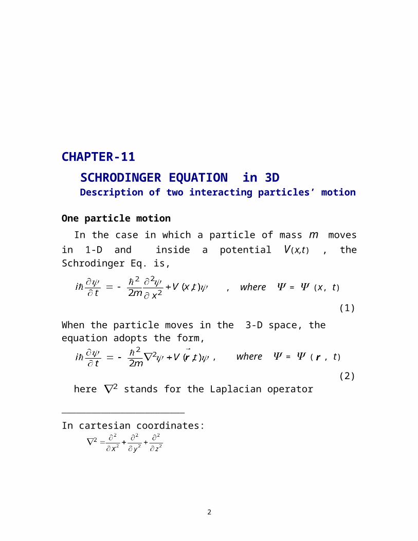
One particle motionIn the case in which a particle of mass m moves in 1-D and inside

a potential V(x,t) , the Schrodinger Eq. is,

, where = (x, t) (1)

When the particle moves in the 3-D space, the equation adopts the form,

, where = ( , t) (2)

here stands for the Laplacian operator

_________________________

In cartesian coordinates:

In spherical coordinates:

11.1 General case of an arbitrary interaction potentialTwo particles motion

2

The mutual interaction between the two particles is specified through the potential and the corresponding Schrodinger Eq. is

, (3)

where = ( t)

In the expression above the following notation is being used,

; ; etc

11.2 Case when the potential depends only on the relative position of the particles

Here we consider that the potential depends only on the relative position,

= (4)

Decoupling the Center of Mass motion and the Relative MotionFor this particular case it can be shown that the motion of the two particles can be decoupled into

the motion of the center of mass, and the motion relative to each other.

The CM and the relative-position variablesSuch decoupling can be achieved through the following change of variables:

, (5)

( t) = ( t)

3

Notice, by calling and

the definitions in (5) can be re-written more explicitly as,

, ,

, , (6)

( t) = ( t)

where we are using _________________________

You may want to jump to expression (10), which gives the form in which Eq. (3) is transformed upon the application of the change of variable (5). ( t) = ( t) implies,

4

Since , adding the last three results gives,

where we have used the notation

, and

,

Very conveniently, the previous results is expressed as,

(7)

Similarly

Analogous results for and lead to,

(8)

5

Replacing (7) and (8) in (3) one obtains,

In terms the reduced mass

(9)

one obtains the equation

(10)

where = ( t)

Solution by separation of variablesWe will specialize in the case where the potential does not depend explicitly on the time t. For such a case, we will be looking for solutions to Eq. (10) in the form,

( t) ≡ (11)

Replacing (11) in (10)

Dividing by

This expression indicates that the terms on the right, although intrinsically depending on the variables and , they add up to a constant value. Selectively we choose,

6

, (12)

and

(13)

Equation of Motion for the Center of Mass The first expression leads to,

(14)

which admit solutions of the form

(15)

where is an arbitrary constant unit vector. (That means there are many solutions of this type, one for each selected unit vector .)

In terms of the wavevector , the previous expression is written as,

= (15)’

In short, if a single vector were used in the separation of variables

given in (11), then the motion of the CM would be described by a plane-wave that propagates in the direction of ,

(16)

Accordingly, the CM is likely to be anywhere in the space but has a very definite orientation of its momentum (that given by ).

If a more precise localization of the CM were desired, then we can select a bunch of wavevectors within a range

and define a wavepacket

. (17)

7

That way the CM will be more localized (because is more spatially localized) but, at the same time, there will be a corresponding uncertainty in its momentum.

It is worth mentioning that we have not been looking for a solution , as we would have been doing in a classical mechanics

approach; rather we have found an amplitude probability .

Equation governing the Relative Motion

Back to Eq. (13). This leads to,

(18)

In the next section we will specialize for the case for central potentials; that is, when the potential depends only on the magnitude of the particles separation:

11.3 Central Potentials (19)

This is an equation for where the energy parameter E is still to be determined. When working with central potentials, it is more convenient to use spherical coordinates to solve (19).At the beginning of this Chapter the Laplacian operator was given in spherical coordinates. Using that expression in (19) one obtains,

(20)

11.3A Separation of variables method We will look for solutions of the form

(21)

8

This leads to,

Dividing each term by

+

+

+

The first two terms depend only on r, while the third term only on the angular variables. This means that the radial part and the angular part are each constant.

Rearranging terms, one obtains

9

Angular Eq. (22)

and

Radial Eq. (23)

11.3B The angular Equation To solve the angular equation

we will look for solutions of the form,(24)

+ =

Dividing by and multiplying by sin2()

[ + sin2() ] + = 0

This means that each of the two term must be constant

[ + sin2() ] = m2 (25)

= - m2 (26)

The value of the constant m2 is determined by physics-based considerations. Indeed, from the second Eq. above one obtains

+ m2 = 0

10

(where the partial derivative symbol has been dropped, since the function depends only on one variable,) which has solutions of the form =ei

m. But notice that the wavefunction should take the

same value whenever is incremented by 2; that is,

= (physics-based requirement)

This implies ei m( = ei

m, or

ei m = 1

This condition can be satisfied only if m is an integer number. Thus, the dependence of the wavefunction on the variable is given by,

= ei m ; m = … , -2, -1, 0, 1, 2, … (27)

where the factor ( 1/ ) has been introduced to ensure the ortho-normality condition of these functions in the range ,

(28)

The other angular Equation (25) has the form,

(29)

where it has been emphasized that the solution depends on the parameters and m. The task is to find a solution over the range 0 ≤ ≤ . It is convenient introduce the new variable

w = cos (), for 0 ≤ ≤.

11

and the new function

Fm (w) =

It can be shown that the Eq. for Fm is,

(30)

Case m=0We will see later that the functions Fm corresponding to m≠0 can be built upon F0 . The latter satisfies the Eq.

Legendre Eq. (31)

Power series solution

F0 (w) = (32)

From (31) one obtains,

, , which gives,

+ =

(33)

Also,

,

-

= -

Using k - 2 = k’

12

= -

where we have replaced k’ for k again (to avoid writing too many variables)

= (34)

Replacing (33) and (34) in (31), one obtains

+ = 0

= 0

This requires

recursion relation (35)

Thus, the solution (32) can be written more explicitly as,

F0 (w) = (36)

+

where and are arbitrary constants. Expression (31) provides two independent solutions. Notice, each subsequent coefficient depends on the value of the previous one (for example, if one coefficient were equal to zero, then all the other subsequent coefficients will be null as well.)

Divergence at w =1. For large values of k, this series varies as , a behavior which is similar to the divergent series

. This indicates that (32) diverges for w=1, thus constituting

an unacceptable solution, since the wavefunction has to have a definite value at =90o.

Polynomial solutions. It is still possible to obtain a satisfactory solution out of (32), if were chosen of the form = l (l +1), with l being an integer value, then the coefficient series (32) would become a polynomial of degree l (with the corresponding or

13

conveniently chosen equal to zero, depending on whether l is odd or even, respectively.)

Summary:The Legendre Eq

Legendre Eq.

admits physically acceptable solutions provided that has the form of = l (l +1), with l being an integer. For a given l, the resulting solutions is a polynomial of degree l.

F0 (w) = Legendre Polyniomial .

where

Since an arbitrary multiplicative constant, or , accompany to these solutions, the Legendre polynomials are defined such that

Pl (1) =1

From expression (36) one obtains,

l = 0: (37)

l = 1:

l = 2:

l = 3:

l = 4:…

Since Pl is a polynomial of degree l,Pl (-w) = (-1)l Pl (w) (38)

14

Without proof we state that the Legendre polynomials satisfy,

(39)

The general case: m≠ 0We are looking for solutions to Eq. (29)

For that purpose, let’s define the Associated Legendre functions

(40)

That is, the polynomials are obtained by taking derivatives of

the already known Legendre polynomials given in (37). It turns out these Associated Legendre functions satisfy Eq. (29),

(41)

Notice that, since is a polynomial of degree l , will

be identically equal to zero for . Accordingly, for a given l there will be (2 l + 1) associated Legendre polynomials

m = - l , - l +1, … , l -1, l (42)

Using the Legendre polynomials given in (37) one obtains,

l = 0, m= 0: (43)

l = 1, m= 0:

15

m= 1:

l = 2, m= 0:

m= 1:

m= 2:

Since is a polynomial of degree ( l - ) and ,

is an even function, then

(44)

Without proof we state that the associated Legendre polynomials satisfy,

(45)

This expression will be useful for properly normalizing the wavefunction.

Summary: The angular equation (22)

Admits solutions of the form:

= , l = 0, 1, 2, 3, …

= ei m ; m = - l, … , -1, 0, 1, … , l

A proper constant in front of is selected so that the solutions are normalized:

16

Spherical Harmonics

for

(46)

The factor (-1)m is chosen for convenience (other authors’ notation differ by a factor of (i)l .)

The spherical harmonics constitute an orthonormal set of functions

(47)

The following sebsitei s very helpful to visualize the harmonic functions:http://www.vis.uni-stuttgart.de/~kraus/LiveGraphics3D/java_script/SphericalHarmonics.html

Absolute value of real part l=0, m=0

Absolute value, colored by complex phase l=0, m=0 ____________________________________

17

l = 1, m= 0 l =1, m=1Absolute value of real part

l =1, m=0 l =1, m=1Absolute value, colored by complex phase____________________________________

18

l = 2, m= 0 l =2, m=1 l =2, m=2Absolute value of real part (illuminated by light.)

l =2, m=0 l =2, m=1 l =2, m=2Absolute value, colored by complex phase

____________________________________

11.3B The Radial Equation We have found that in Eq. (23) = l ( l+1 )

19

For the case of a Coulomb field

where , Z is the atomic number (number of

protons in the nucleus) and e is the elementary charge,

the Eq. is,

When considering the case of a Coulomb field, it is convenient to use

as the units of mass, length and time, respectively.

Notice that the unit of energy is .

For our purpose, instead of we will use the reduced mass

instead. Thus, since has units of distance, and has units of

energy, the equation above can be expressed in terms of unit-less parameters r’ and E’ instead of the variables r and E, where

r ≡ r’ , E ≡ E’ .

Indeed, using in addition R(r)= R(r’), , … etc.,

one obtains,

20

Let

R(r’) =

The purpose of this change of variable is to obtain an equation the resembles the one dimensional case.

Adding the last two expressions

This Eq. can be expressed as,

where an effective potential has been defined as,

Looking for bound statesBound states will be obtained with negative values for E’.

21

Let’s define

and

u(r’)=v() , ,

22