biology, ecology, and management of deer in the chicago
TRANSCRIPT

I L L INO SUNIVERSITY OF ILLINOIS AT URBANA-CHAMPAIGN
PRODUCTION NOTE
University of Illinois atUrbana-Champaign Library
Large-scale Digitization Project, 2007.


ILLINOIS
C"4 %r - x 7
HISTORY -F Pr I
~L tQVLY
TER FOR WILDLIFE ECOLOGYf, ECOLOGY, AND MANAGEMENT OF DEER IN THE
CHICAGO METROPOLITAN AREA
Project Number W-87-R
Final Report
by
James H. Witham and Jon M. JonesIllinois Natural History Survey
1 February 1992
S k ^mr " rr IXA I UrrLi


Final ReportSubmitted to
ILLINOIS DEPARTMENT OF CONSERVATIONDIVISION OF WILDLIFE RESOURCES
Project Number W-87-RBiology, Ecology, and Management of Deer in the
Chicago Metropolitan Area
by
James H. Witham and Jon M. Jones1 February 1992

TABLE OF CONTENTSPage
TABLE OF CONTENTS. .................................................. 1
INTRODUCTION. .................................................... ... 1
PROJECT OBJECTIVES .............................................. 4
STUDY AREAS......................................................... 5Chicago Metropolitan Area.......................................... 5Ned Brown Preserve. .............................................. 9Chicago-O'Hare International Airport.............................. 10Ryerson Conservation Area.......................................... 11
Study No. 104-1: Life History and Ecology of Urban Deer............ 12Population parameters ......................................... 12Deer abundance .............................................. 12Deer counts: Cook, DuPage, and Lake counties.................. 12Deer counts Kane County.....................................14Reproductive performance and fetal sex ratio................... 14Survival rates.. ... ........................................ 14Age composition and longevity of deer removed from Ned Brown..... 15Deer health.................................................16Health/condition evaluations.....................................16Relative condition of deer on forest preserves................. 16Body composition/condition of fawns............................. 18Body composition change of fawns during winter.................. 18Estimating fawn body composition with deuterium oxide........... 19Parasites of urban deer...................................... 19Helminthic and protozoan parasites...........................19Histopathology. ........................................... 19California encephalitis: Jamestown Canyon virus................ 19Lyme disease ............................................... 20
Study No. 104-2s Deer Range Evaluation.......................... 20Effects of deer on forest vegetation. .......................... 20Historical perspective and objectives.......................... 20Plant measurements............................................ 23Busse exclosure and control plot...............................23Busse Nature Preserve: plants < lm............................. 24Busse Nature Preserves shrubs and saplings > la................ 25Other coparative measurements.................................25
Deer habitat evaluations........................................ 26Landsat satellite imagery evaluation............................. 26Changes in land uses Insularity of Ned Brown Preserve........... 27Deer-vehicle accidents............................................ 28Accident costs................................................... 28Distribution of accidents and regional trends.................... 29
i

Study No. 104-3: Management Strategies and Control................. 30Experimental deer herd reductions................................ 30Deer reductions at Ned Brown Preserve............................ 30Background information........................................ 30Management plan and evaluations................................ 32Chicago-O'Hare International Airport............................. 33Background information...................................... 34Management plan and evaluations................................ 35Ryerson Conservation Area.................................... 35Background information....................................... 36Management plan and evaluations................................ 39Translocation of metropolitan deer.............................. 40
Study No. 104-4: Data Management, Analysis and Reporting........... 41
RESULTS ............................................................ 41
Study No. 104-1: Life History and Ecology of Urban Deer........... 41Population parameters........................................ 41Deer abundance.... ......................................... 41Deer counts: Cook, DuPage, and Lake counties.................. 41Deer count: Kane County..................................... 42Reproductive performance and fetal sex ratio................... 43Survival rates......... .................................... 44Age composition and longevity of deer removed from Ned Brown..... 45
Deer health.......... .. ................................... 46Health/condition evaluations................................. 46Relative condition of deer on forest preserves................ 46Body composition/condition of fawns.......................... 49Body composition change of fawns during winter................ 50Estimating fawn body composition with deuterium oxide........... 50
Parasites of urban deer...................................... 51Helminthic and protozoan parasites........................... 51Histopathology.............................................. 51California encephalitis: Jamestown Canyon virus................ 53
Study No. 104-2: Deer Range Evaluation.......................... 53Effects of deer on forest vegetation........................... 53Historical perspective and objectives............................ 53Plant measurements...........................................53Busse exclosure and control plot............................ 53Busse Nature Preserve: plants < 1m.......................... 56Busse Nature Preserves shrubs and saplings > m................ 57Busse Nature Preserve vs. Busse Woods South.................. 60
Deer habitat evaluations....................................... 60Landsat satellite imagery evaluation............................. 60Changes in land use: Insularity of Ned Brown Preserve............ 61Deer-vehicle accidents......................................... 62Accident costs.............. .................................. 62Distribution of accidents and regional trends.................... 63
ii

Study No. 104-3: Management Strategies and Control................. 64Experimental deer herd reductions................................ 64Deer reductions at Ned Brown Preserve............................ 64Chicago-O'Hare International Airport............................ 67Ryerson Conservation Area.............. ........................ 69Translocation of metropolitan deer............................... 73Alternatives: Population control and damage abatement........... 73
Study No. 104-4: Data Management, Analysis and Reporting..... ... 75Database management and transfer of records to DOC................ 75Transfer of project information to organizations and publics...... 76Print media...................................................... 76Radio media .................................................. 77Television media ............................................ 77Reports produced from this study............................... 77Publications produced from this study.......................... 77
DISCUSSIO......................................................78
Deer health and insular preserves............................... 78Prognosis, Plant community recovery at the Ned Brown Preserve...... 82On urban deer management: the role of a state wildlife agency*...... 92
LITERATURE CITED................................................. 95
TABIESLIST O FIGURES
FIGURES
APPDICES
iii

INTRODUCTION
The white-tailed deer (Odocoileus virqinianus) is the most extensively
managed ungulate in North American and has been the subject of continuous
research for >50 years (Halls 1984). Management goals to restore whitetail
abundance and distribution have been realized on most historic North American
deer range. Modern deer population management attempts, in part, to regulate
long term deer densities at levels compatible with range conditions or land uses
by offsetting annual recruitment with recreational hunting mortality. This
system of deer management is most effective in rural settings where human
densities are low, average property size is large, and hunting is a tradition.
However, large numbers of deer also inhabit many suburban and suburban-rural
fringe areas where their close proximity to people inevitably results in various
conflicts. Metro environments contrast with rural areas in that human densities
are high, property ownership is finely subdivided, and most residents do not
participate in hunting (Kellert 1980). An increasing number of natural resource
agencies are now faced with deciding how to address deer-human conflicts in metro
areas.
Deer at moderate to high densities are not compatible with all land uses
in metro environments which have been modified for, and dominated by, people.
Unquestionably, urbanites value the presence of deer (Connelly et al. 1987,
Decker and Gavin 1987), in part, because deer are large bodied, easily observed,
nonthreatening, herbivores that are a "natural antithesis" to typical city life.
Such appreciation, however, is conditional and depends on the willingness of
people to tolerate, or to effectively mitigate, the adverse consequences (e.g.,
accidents, floral damage, ecological damage) that inevitably recur when deer and

people occupy comon land.
The principal goal of deer management in metropolitan areas is to limit
damage caused by deer within a range that is acceptable to residents and/or
compatible with local land use, yet maintain deer populations high enough to
retain the positive values associated with the presence of deer. Finding and
achieving this balance is difficult because metropolitan residents possess
diverse and conflicting interests, values, perceptions, and knowledge of wildlife
(Kellert 1980). Because of inherently strong social interest, metropolitan deer
issues are often intense, highly politicized, and covered extensively by media.
Under conditions such as these, achieving consensus on how to address deer-human
conflicts may be far more difficult than physically implementing any management
program that is selected.
Deer in the CHA received limited, informal study prior to 1983. We found
no published data on deer in the CMA and only several informal intradepartmental
sumaries. For example, Cook County naturalists examined several hundred deer
killed by vehicles from 1968 to 1977, but published no reports (Schwarz, Cook Co.
For. Pres. Dist., pers. comun., 1983); the IDOC and U.S. Fish and Wildlife
Service kept minimal records of deer removed from Chicago-O'Hare International
Airport during 1982-1983 (Loomis, IDOC, pers. com'un., 1984); and, the locations
of deer-vehicle accidents on sections of 2 tollways were evaluated by the
Illinois State Police (Burns, Ill. St. Police, unpub. rep., 1984). Other deer
studies conducted in more rural areas of central and southern Illinois (e.g.,
Nixon et al. 1991, Roseberry and Woolf 1991) are important contributions for our
understanding of deer management and ecology in Illinois, but do not address deer
management needs that are specific to metropolitan northeast Illinois. Because
data necessary for metro deer management were inadequate, the IDOC contracted the

3
Illinois Natural History Survey (INHS) to study whitetail ecology and management
in the CHA from 1983 to 1989.
Research goals of the INHS Urban Deer Study were to collect baseline data
that would be useful for deer management and to perform short-term, experimental,
reductions of deer populations on selected sites that would set precedence for
long-term deer management in metropolitan areas of Illinois.
Various substudies were initiated as part of the INHS Urban Deer Study
since its inception in 1983. This job completion report includes some extended
abstracts that are supported by appended manuscripts. Other substudies are
summarized entirely within the text. All work reported in the methods and
results sections are segregated by their respective contract Job numbers (i.e.,
Job No. 104-1 to 104-4) which are listed as objectives on page 4.
Acknowledgments
The authors thank the many people and organizations that contributed tovarious segments of this program. Specifically, we thank personnel of theIllinois Natural History Surveys Dr. Glen Sanderson, James Seets, Kathy Lee,Janet Rachlow, Dr. William Edwards, Dr. Richard Warner, Elizabeth Cook, ElizabethAnderson, Larry Gross, Monica Lusk, Carla Heister, and Jose Cisneros; theIllinois Department of Conservation: Dr. John Tranquilli, Jeffrey Ver Steeg, andForrest Loomis; the Cook County Forest Preserve Districts Raymond Schwarz, ChrisAnchor, and Arthur Janura; the Lake County Forest Preserve Districts DanBrouillard; the Chicago Zoological Society-Brookfield Zoo: Dr. Bruce Watkins; theIllinois Department of Transportation EMS helicopter pilots and Gene Milliron;and Chicago-O'Hare International Airport Department of Aviation Safety: RussellGebhardt.

4
States Illinois Project Numbers W-87-R
Project Types Research
Project Titles Cooperative Forest Wildlife Research
Sub-Project VII-Ds Biology, Ecology, and Management of Deer inthe Chicago Metropolitan Area
Study No. 104-1s Life History and Ecology of an Urban Deer Herd
Study Objectivess To investigate and quantify pertinent aspects of lifehistory, ecology, health, abundance, dynamics, and distribution of deer inmetropolitan areas of northeastern Illinois relative and necessary totheir successful management.
Study No. 104-2s Deer Range Evaluation for MetropolitanNortheastern Illinois
Study Objectives: To measure, map, and otherwise quantify and qualify thepresent and potential deer range of northeastern Illinois includingassessments of present impacts of deer on vegetation.
Study No. 104-31 Management Strategies and Imlementation of xperimentalControl of Urban Deer
Study Objectivess To design, implement, and evaluate possible alternativestrategies for management of deer in urban areas with special respect tonortheastern Illinois. Pilot management programs to be undertaken ascooperative programs with the Illinois Department of Conservation andlocal public agencies sustaining significant deer problems.
Study No. 104-41 Data Base Management. Analysis, and Reporting on UrbanDeer Research
Study Objectives: To compile, organize, computerize, and manage for readyaccess, security, and preservation all data resulting from this studyrelating to deer, deer range, and other aspects of natural resourceinformation generated by this project. Data to be integrated into database management system. To generate file and manuscript reports,scientific and professional manuscripts for publication, and news releasesfor local and statewide distribution.
5
Chicago Metropolitan Area (COA)
The 5900 km2 study area included Cook, DuPage, Kane, and Lake counties
in northeastern Illinois (Fig. 1). These counties were selected for study
because of their metropolitan characteristics and because they are the only
counties in Illinois that are closed to firearm hunting for deer. HcHenry and
Will counties, which are normally considered as part of the CHA, were excluded
from the study area because deer were legally hunted with firearms during
regulated hunting seasons. All Illinois counties were open to archery hunting
for deer during the 3-month autumn season. On county-owned preserves in the
CHA where there were large concentrations of deer, county ordinances
prohibited hunting of any type. Thus, our study area was selected, in part,
because social and political influences limited hunting as a means for
regulating deer abundance and abating deer-related property damage.
Climate in northeastern Illinois is predominately temperate continental
with warm, humid summers and cold winters. Local weather changes rapidly and
is influenced by the proximity of a site to Lake Michigan which ameliorates
temperature extremes, modifies wind patterns, and produces lake-effect
precipitation. Average daily maximum temperature during July is 28.5 C.
Lowest average daily minimum temperatures occur during December (-6.5 C),
January (-10.2 C), and February (-7.7 C). Mean annual precipitation and
snowfall are 89.7 cm and 101.1 ca, respectively (Natl. Oceanic and Atmospheric
Admin., 1987).
Average daily temperature by month, annual precipitation, and annual
snowfall from 1983 to 1988 were compared with 30-year normals determined from

1958 to 1987. Winter temperature varied substantially among years, for
examples colder than normal temperatures during winter 1983-84 were temporally
interrupted by an exceptionally warm February, colder than normal winter
temperatures during 1984-85 and 1987-88 were limited to January and February,
and temperatures during each month during winters 1982-83 and 1986-87 exceeded
normals. For the 30-year period in which normals were calculated, both the
highest (1987) and lowest (1985) average annual temperatures occurred during
our study. Total annual precipitation alternated above and below normal
values during the study. Total precipitation during 1983 was 39% higher than
normal and was the wettest year during the previous 30 years. Snowfall
exceeded normal during 2 of 6 years with the greatest amount occurring the
first winter of the study (1983-84). Snowfall during 3 winters (i.e.. 1982-
83, 1985-86. 1986-87) was > 25.0 ca below normal.
Total population size for the CMA was 6,855,400 people in 1988. Host
people (5.284,300) live in Cook County which includes the City of Chicago
(2,977,520 people). Residents in DuPage (760,800), Kane (315,000), and Lake
(495,300) counties comprised 23% of the CHA population (1 July 1988 estimate,
Northeast Ill. Planning Corm. 1989). Human densities by county ranged from
232 people/ka2 (Kane) to 2.132 people/km2 (Cook).
Land cover in the CMA was estimated by E.A. Cook (Illinois Natural
History Survey, Champaign) based on Landsat Thematic Mapper data collected 27
June 1988. Counties in the CMA were a gradient of urbanization. Percent
cover in urban or residential-use by county ranged from 29% (Kane) to 76%
(Cook) and collectively was 57% for the CHA. Percent cropland by county was a
reverse gradient of urbanization ranging from Cook County (5%) to more rural
Kane County (51%). Trees were present on 25% of the CMA as undeveloped
forests, savannas, or residential areas with canopy closure >30%. Percent
forest cover was highest in urbanized Cook (30%) and DuPage (31%) counties.
Undeveloped forest cover, important as thermal and concealment cover for
-midwest whitetails during winter (Gladfelter 1984), was comparable in Lake
(8%) and Cook (8%), but lower in DuPage (5%) and Kane (4%) counties. More
rural counties sustained highest net reductions (8 to 9% from 1985-1988) in
deer habitat which resulted primarily from conversion of agriculture to urban
uses.
The physiography of northeastern Illinois is well documented (Leighton
et al. 1948, Willman 1971, Mapes 1979, and others). The CMA is part of the
Great Lake and Till Plains sections of the Central Lowland physiographic
province. Illinoian and Wisconsinan glaciation during the Pleistocene created
the gently rolling to near level topography of northern Illinois. Soils are
derived primarily from deposits of glacial till, outwash sands, and lake-bed
sediments, and were described to the association level by Fehrenbacher et al.
1984. Based on physiographic and biotic community similarities, Schwegman
(1973) included the study area in the Northeastern Morainal Division of
Ilinois, except for southwest Kane County, which is in the Grand Prairie
Division.
Swink and Wilhelm (1979) described species, associations, and
distribution of native vascular plants in the Chicago region. Schmid (1975)
discussed the complex processes (e.g., socioeconomic, climatic) that
interacted to produce present-day urban vegetation in Chicago. Spatial and
temporal trends in forest resources by counties in Illinois were analyzed by
Iverson et al. 1989. Illinois flora were described by Jones (1963) and
Mohlenbrock (1975) and are listed on a permanent computer data base (i.e.,

Illinois Plant Information Network; Iverson and Ketzner 1988).
From the early 1800's to present, people have progressively altered
Illinois landscape, initially with conversion of prairie to agriculture,
logging, and grazing, and more recently with sustained urbanization.
Potential major natural vegetative communities in northeastern Illinois were
bluestem (Andropogon spp.) prairie, oak (Quercus spp.)/hickory (Carya spp.),
maple (Acer spp.)/basswood (Tilia americana) and oak savannah (Kuchler 1964);
however, the intensive land use that typifies this area has left only remnants
of these communities. Less than 0.0007 of natural communities that existed in
presettlement Illinois remain in a condition of high natural quality (White
1978). The response of people and governments to these state-wide
perturbations has been to purchase properties for open space on the periphery
of urban centers and to protect remnant natural areas that are representative
of presettlement natural communities. Open space properties that are owned by
county governments are named "forest preserves" (Wendling et al. 1981). The
Cook County Forest Preserve District was officially established in 1914 and
charged to$
"...acquire...and hold lands...containing one or more natural forests orlands connecting such forests or parts thereof, for the purpose ofprotecting and preserving the flora, fauna, and scenic beauties withinsuch district, and to restore, restock, protect, and preserve the naturalforests and said lands together with their flora and fauna, as nearly asmay be, in their natural state and condition, for the purpose of theeducation, pleasure, and recreation of the public" (Forest PreserveDistrict of Cook County, 1918).
Following Cook County, forest preserve districts were established in
DuPage, Lake, and Kane counties. By 1988, approximately 7% of the CMA was
owned and managed by county forest preserve districts.
Some natural areas are protected as part of the Illinois Nature

Preserves System and are managed for long term ecosystem preservation (Ill.
Admin. Code, Title 17, Chapt. V, Part 4000, Management of Nature Preserves).
"Nature preserves" are owned by a variety of public and private interests who
have legally dedicated, in perpetuity, the protection of their properties
against disturbances (Witter 1987). Thus. a county-owned "forest preserve"
can also be dedicated as a State Nature Preserve. Two of the INHS study
areas, the Ned Brown Preserve and Ryerson Conservation Area, were county
forest preserves with parts of their holdings dedicated as State Nature
Preserves (i.e., Busse Forest Nature Preserve and Ryerson Nature Preserve,
respectively). Busse Forest is further recognized by the U.S. National Park
Service as a Registered Federal Natural Landmark which identifies the site as
an area of national ecological significance.
Ned Brown Preserve and Busse Forest Nature Preserve
The 1,536 ha Ned Brown Preserve, owned and managed by the Cook County
Forest Preserve District, is located in northwest Cook County near Elk Grove
Village. Land use adjacent to the Ned Brown Preserve includes several large
indoor shopping malls, 2 tollways, 2 state highways, residential developments,
and corporate buildings. More than 20 high rise buildings are <1 km from the
preserve. Airspace is within the Chicago-0'Hare International Airport
Terminal Control Area with jet traffic frequently passing over the preserve on
final approach at 800 m AGL. The Ned Brown Preserve was developed for
recreational use with paved bike trails, picnic groves, a model airplane
flying field, and a 241-ha reservoir with recreation facilities. More than
1.5 million visitors used the preserve during 1985 (Dwyer et al. 1985). The
Ned Brown Preserve is 66% woodland dominated by oak (Quercus spp.), sugar

10
maple (Acer saccharum), and basswood (Tilia americana), 10% in old field
successional stages, wetlands, and mowed grass; 15% in open water, and 9% in
roads and other developments. Quantitative evaluations of vegetation at Ned
Brown were a major part of this study are reported elsewhere (pages 20 & 54).
Within the Ned Brown Preserve is the 177-ha Busse Forest Nature
Preserve. The site is a dedicated Illinois Nature Preserve and Registered
Federal Natural Landmark. The latter is recognition from the U.S. National
Park Service as an ecological site of national significance. The preserve is
comprised of 5 natural communitiess a high quality dry mesic upland forest,
mesic upland forest, mesic hardwood, northern flatwoods, and shrub
swamp/marsh.
Chicago-O'Hare International Airport
The 3,116 (7,700 ac) Chicago-0'Hare International Airport (O'Hare) is
owned and operated by the City of Chicago Department of Aviation. It is a
major commercial aviation facility that serves over 50 airlines and averages
110 arrivals/departures each hour. The airport facility is dominated by a
complex system of highways, parking lots, terminals, support buildings, and
runways (typescript O'Hare Factsheet 7/90). About 650 ha of undeveloped
property lies near runways and on the airport periphery. This undeveloped
property is comprised of early second growth (i.e., shrubs and saplings)
woodlots, a mixture of early successional fields, swamp/marsh, 3 tree
nurseries maintained for the Chicago Park District, and mowed grassland near
runways.
Aerial photographs of O'Hare and adjacent properties were reviewed for
1949, 1963, 1975, and 1985. The sequence of photographs showed successional
11
changes in vegetation that increased quality and quantity of deer habitat on
undeveloped airport property. The agricultural-influenced landscape of 1949
had by 1985 evolved into a more structurally diverse mixture of plant
communities which has favored establishment and increase of deer. Conversely,
during the same period, most private property immediately north, west, and
south of O'Hare was developed for residential, commercial, and industrial
uses. East of the airport, separated by a 1.3 to 2.0 km strip of commercial
development, are county forest preserves which sustain deer herds at >15
deer/km2 (Witham and Jones, this study).
Ryerson Conservation Area and Ryerson Nature Preserve
Ryerson Conservation Area (Ryerson) is a 223-ha preserve within the Lake
County Forest Preserve District (LCFPD) which included 27 preserves totaling
5,368 ha (range 7-562 ha) in 1990. Ryerson is located 50 km north of Chicago
in southeastern Lake County near the village of Deerfield.
Historic land use at Ryerson was reviewed by Nuzzo (1988). Permanent
settlement occurred in 1834 with an active sawmill operating from 1835-1870
near the southern property boundary. Timber lots (2-8 ha each) were purchased
by nearby farmers in the 1850's and used for cattle grazing and timber
production. In the 1890's, an amusement park was built on the southern part
of the preserve, but was discontinued before 1915. The timber lots were sold
in the 1920's to Chicago residents who used these sites as vacation retreats.
Edward L. Ryerson purchased land in this area from 1927 to 1939. From 1966 to
1972, acting to protect the continuity and natural qualities of their
properties, Ryerson and other landholders donated their estates to the Lake
County Forest Preserve District. These donated properties comprise the

12
Ryerson Conservation Area; 2 high quality natural areas (61 and 52 contiguous
ha) within the RCA were dedicated as the Edward L. Ryerson Nature Preserve
(RNP) on 27 April 1972 and 21 May 1979. respectively.
Nuzzo (1988) described the climate, physiography, geology, soils.
hydrology, biota, and significant natural features of RCA. The RNP is
comprised of 9 natural communitiess dry-mesic upland forest (white oak-swamp
white oak-sugar maple), aesic upland forest (sugar maple-basswood-red oak),
mesic floodplain forest (sugar maple-basswood-red oak), wet-mesic floodplain
forest (silver maple-bur oak-swamp white oak), wet floodplain forest (silver
maple-cottonwood-boxelder), northern flatwoods (swamp white oak), sedge meadow
(sedges-bullrushes), fen, and low-gradient river.
METHODS
Study No. 104-1: Life History and Ecology of an Urban Deer Herd
Population parameters
Deer abundance
Deer counts» Cook. DuPage. and Lake counties.-- Deer were counted in
Cook. DuPage, and/or Lake counties from a Cessna 172 fixed-wing aircraft
during 1984-1985 and from a Bell Long-Ranger helicopter during 1985-1988. The
helicopter was favored because of greater maneuverability and improved safety
while flying at low altitudes (90-150 m AGL) and reduced speeds (50-60 knots)
over developed areas and near major airports. Areas with vegetative cover
that was relatively homogeneous were surveyed systematically by flying
parallel transects determined by aircraft instrumentation and visual ground
references. Transect widths were not measured, but we estimate that they
varied from 100 m in mature forests to 300 m for agricultural fields without

13
standing crops. We divided smaller preserves, and areas with heterogeneous
vegetative cover types, into subunits with boundaries that were defined by
natural features (e.g., changes in vegetation, rivers, lakes) and roads that
were visible from the air; we searched these subunits systematically and then
totaled all nonduplicate deer counted within each preserve. Individual
preserves were surveyed 5 1 time annually and from 1 to 5 times during the
study. Surveys were conducted during winter when snow depth exceeded 10 cm.
Two observers in verbal contact counted deer from 1 side of the aircraft.
Our aerial counts reflect the maximum number of independent observations
of deer that we made on each site at the time of the census only. We deleted
observations where duplicate sightings may have occurred. These included deer
that were disturbed by the aircraft and traveled into areas yet to be
surveyed. Most deer observed during surveys remained stationary or moved <50
a toward cover or other deer. Because many factors preclude counting all deer
on a site, we refer to data based on our counts as "inimum" numbers or
"minimum" densities.
We divided the number of deer counted by forest preserve area to
determine deer densities. Areal measurements of sizes of individual preserves
DuPage and Lake counties were provided by their forest preserve districts.
Sizes of preserves in Cook County were determined with a dot grid overlaid on
forest preserve maps. Contiguous preserves were divided into subunits defined
by administrative boundaries, bisecting roads, or other features that were
readily visible from the air.
For the purpose of publication, we redefined preserves by contiguity of
property irrespective of administrative divisions (e.g., preserves on the Des
Plaines River in Cook and Lake counties were considered as 1 large preserve)

14
and then estimated minimum deer densities for these areas. The objective was
to determine the minimum number of deer on selected metropolitan forest
preserves during winter. The abstract is listed in Results (page 41) and the
publication (Witham and Jones 1990) is Appendix A.
Deer count: Kane County.--Deer in Kane County were counted by 2
observers in a fixed-wing aircraft during January 1987. Unlike censuses in
Cook, DuPage, and Lake counties where deer were counted only on forest
preserve properties, the 2-day count in Kane County included all county land
west of the Fox River. Complete coverage was possible for this area because
the landscape is dominated by open agricultural fields and had relatively less
woodland than other counties within the study area. The objective of this
survey was to estimate winter distribution of deer, only.
Reproductive performance and fetal sex ratio
We compared fecundity among fawn, yearling, and adult does that were
collected from Ned Brown, Des Plaines, Palos, Northwest Cook, and Non-Cook
areas, during 1983-1985. Fetuses were counted and sexed during postmortem
examinations during January-May. Does were separated into fawn, yearling, and
adult age classes, based on wear and replacement of dentition. We examined
the reproductive tracts of does collected at the Ned Brown Preserve annually
until 1989.
Survival rates
Deer were live captured and released at the Ned Brown Preserve during 2
winters. All deer received an aluminum tag in each ear. Does were fitted
with black plastic neck collars that were marked with numbers or letters made
from colored reflector material. Bucks were uniquely marked in both ears with
color-coded, plastic cattle-tags and streamers. Thus, each deer could be

15
individually recognized at a distance during subsequent field work which
included spotlight counts, live capture, and sharpshooting. Some deer were
never observed after release; however, most (94/103, 91%) deer were reobserved
or their fates were determined through tag returns. The small size of Ned
Brown Preserve (1,536 ha), extensive use by recreationists, intensive
fieldwork by INHS, and cooperation from local police departments and county
personnel who reported deer mortalities to INHS, increased our ability to
determine the status of marked deer.
Although the 103 deer that were live captured in this study segment were
not radio collared, the high percentage of marked deer that we reobserved at
Ned Brown enabled us to use Program MICROMORT (Heisey 1985) to estimate
survival rates. Survival rates of fawns, yearlings, and adults, were
calculated by 6-month intervals. Only marked deer that were known to be alive
at the beginning of a time period were used in the analyses. Because some
deer may have died and were not reported to INHS, our estimates represent
maximum survival rates.
Aqe composition and lonevitv of deer removed from the Ned Brown Preserve
Deer that were removed by sharpshooters from the Ned Brown Preserve from
1984 to 1988, were aged by dental wear and replacement (i.e., fawns and
yearlings; Severinghaus 1949) or cementum annuli counts (i.e., adults;
Matson's, Milltown, Mont.). Only adult deer that received "A" or "B"
confidence ratings (i.e., Matson's subjective assessment based on clarity of
ceaentum annuli) were included. By backdating, we reconstructed the composite
age structure of these deer on 1 June 1984.

16
Deer health
Health/condition evaluations
Relative condition of deer on forest preserves.--We contrasted selected
skeletal and body measurements, "fat indices" and reproductive performance of
deer at 5 contiguous areas in the CMA (Fig 2). Our objective was to assess
whether the health of deer differed among preserves that were in close
proximity; detection of area differences would suggest that deer management in
the CMA be scaled for individual preserves. Areas were selected because of
their diverse characteristics relative to development. Four areas were forest
preserves in Cook County and their associated buffer areas. The fifth area
(Non-Cook) included DuPage, Kane and Lake counties, collectively. Two of the
areas in Cook County, the Ned Brown Preserve (Ned Brown) and the Des Plaines
River preserves (Des Plaines) had extensive residential and commercial
development on their peripheries (see page 61). A third site, the Palos-Sag
Valley Preserves (Palos), was partially developed with some adjacent cropland.
The remaining area, including northwest Cook County preserves (Northwest), was
a suburban-rural interface dominated by cropland and estates. The relative
status of areas from most developed to least developed was:
Ned Brown * Des Plaines > Palos > Non-Cook > Northwest
From December 1983 to October 1985, 88 agencies, organizations, and
individuals reported the locations of deer carcasses to INHS. INHS personnel
responded promptly to these reports and removed carcasses, or parts of
carcasses, regardless of condition. The majority of deer collected were
killed or injured by vehicles. In cases where the cause of death was

17
inconclusive, internal trauma revealed during postmortem examinations
suggested that many of these deer were also injured by vehicles. Additional
data were collected from deer that were shot or live-trapped and euthanized by
INHS personnel.
Numerous indices have been used by workers to assess relative skeletal
growth, fat deposition and utilization, and productivity (Watkins et al.
1991). Our selection of 9 indices was influenced by the typical condition of
deer carcasses available (i.e., carcasses with varying trauma). We censored
affected measurements when normal carcass conformation was distorted (e.g.,
bloat, subcutaneous hemorrhaging, skeletal fractures ) or incomplete. Whole
body weight (whole weight) was determined on a "machete counterweight scale"
in 0.45 kg (1.0 lb) increments. Chest girth (girth), right hind foot
(hindfoot), and total body length (total length) were measured in m with a
flexible steel tape using methods of Feldhamer et al. (1985). The right femur
(femur) was incised from the muscle, placed on a flat measurement board, and
measured from the proximal condyle head to the most distal part of the femur.
A left hind foot or left femur measurement was substituted when the right
counterpart was unusable. A skeletal ratio was developed from femur/hindfoot
after Klein (1964). We removed the left kidney and adherent fat to determine
a kidney fat index (KFI) using methods of Riney (1955). Body fat deposition
at 6 locations and musculature were scored using a visual evaluation technique
reported by Kistner et al. (1980). Each deer was aged by tooth wear and
replacement (Severinghaus 1949) and categorized as a fawn (< 1 year),
yearling, or adult (_ 2 years).
To isolate the effects of location, we compared physical measurements
and condition evaluations among deer of similar sex, age class, and season
18
using a 1-way ANOVA. We assumed that observations were independent, that
errors were normally distributed, and that error variances were equal. These
assumptions are plausible because there were no repeated measurements on
individual deer, diagnostics on the subsample of residuals from the 1-way
ANOVA tests indicated that the assumption of normality was reasonable, and
data were categorized by factors that were the main contributors (i.e., sex,
age, season, location) to variations. Data were pooled from both years of
collection and Tukey's test was used to identify differences (P I 0.05).
Body composition/condition evaluation of fawns.-- This is 1 of 3
publications resulting from cooperative studies with the Chicago Zoological
Society. The principal cooperator was Dr. Bruce Watkins, Animal Nutritionist,
Brookfield Zoo, Brookfield, IL. The objective was to determine how various
health indices (i.e., condition) were related to- body size, body composition,
and metabolic status of white-tailed deer fawns collected in the CMA. The
abstract is listed in Results (page 49) and the publication (Watkins et al.
1991) is Appendix B.
Body composition chance of fawns during winter.-- This is the second of
3 publications resulting from cooperative studies with the Chicago Zoological
Society. The principal cooperator was Dr. Bruce Watkins, Animal Nutritionist,
Brookfield Zoo, Brookfield, IL. The objectives were tos 1) to investigate
changes in body composition and chemical component distribution as fawns
underwent net catabolism during winter, and 2) to calculate the composition
and energy content of lost weight based on changes in body composition with
decreasing weight. The abstract is listed in Results (page 50) and the
publication (Watkins et al. 1992) is Appendix C.

19
Estimating fawn body composition with deuterium oxide.-- This is the
last of 3 publications resulting from cooperative studies with the Chicago
Zoological Society. The principal cooperator was Dr. Bruce Watkins, Animal
Nutritionist, Brookfield Zoo, Brookfield, IL. The objective was to evaluate
the efficacy of D20 dilution for predicting body composition of white-tailed
deer fawns under field conditions. The abstract is listed in Results (page
50) and the publication (Watkins et al. 1990) is Appendix D.
Parasites of urban deer
Helminthic and protozoan parasites of urban deer.--Fecal samples were
routinely collected during postmortem evaluations of deer from December 1983
to October 1985. We contracted J.G. Cisneros, a microbiologist whose H.S.
thesis involved examination of deer parasites using fecal flotation methods
(Samuel and Trainer 1969) to examine 270 fecal samples, from deer > 1 year,
for helminthic and protozoan parasites. The abstract is listed in Results
(page 51) and the unpublished report (Cisneros, J.G. 1987. Helminthic and
protozoan parasites of white-tailed deer in urban areas of northeastern
Illinois. Unpub. Rep. Sub. to Ill. Natural History Survey-Wildl. Sec.,
Champaign. 15pp) is Appendix B.
HistopatholoqY.--Lung, liver, and kidney tissue samples were collected
during postmortem evaluations conducted in 1984 and 1985, and submitted for
histopathologic analyses to Dr. John Sundberg, Veterinary Diagnostic
Laboratory, Univ. of Illinois, Champaign. Tissues were fixed in neutral
buffered 10% formalin, embedded in paraffin, sectioned at 6 urn, stained with
hemotoxylin and eosin, and examined for evidence of microscopic pathology.
California encephalitis; Jamestown Canyon virus.--We provided blood sera
from deer live captured in Cook County to Dr. Paul R. Grimstad, Dep. Biology,

20
Univ. Notre Dame, Indiana. Dr. Grimstad evaluated the incidence of infection
of California encephalitis (Jamestown Canyon virus) among 3 deer age classes
(i.e., fawn, yearling & adult).
Lyme disease.-- We did not evaluate Lyme disease in this study.
Callister et al. (1991) surveyed forested areas near Milwaukee, Wisconsin, and
Chicago, for rodents and ticks infected with Borrelia burqdorferi, the
causative agent of Lyme disease. Two voles captured in 1988 near Chicago
tested positive for B. burqdorferi, however, no Ixodes spp. ticks were
captured. The authors hypothesized that B_ burqdorferi is rare in
northeastern Illinois because of the absence of specific tick vectors.
Study No. 104-21 Deer Range Evaluation
Effects of deer on forest vegetation
Historical perspective and objectives
We selected Busse Woods Nature Preserve and the Ned Brown Preserve as a
local study site to evaluate the effects of deer on forest vegetation (Fig.
3). Concerns about the effects that white-tailed deer were having upon the
understory vegetation structure, abundance, and diversity at Busse Woods
Nature Preserve, Cook County Forest Preserve District became prevalent in
1983. Personal observations by laypersons, as well as biologists and
botanists, noted a marked decline in flowering spring ephemerals, the
formation of obvious browse lines, and an abundance of deer.
Baseline data on vegetation within Busse Forest prior to understory
degradation by deer are extremely limited and consist of personal
observations, qualitative assessments conducted by volunteer land stewards for
the Nature Conservancy, and quantitative assessments of cover types, canopy

21
trees, shrubs/saplings, grade or quality of the nature preserve as a natural
area, and qualitative evaluation of the presence of species listed as
endangered or threatened as determined during the Illinois Natural Areas
Inventory (NAI) (White 1978). Observations by volunteer land stewards focused
on the occurrence of herbaceous understory species in 1977-79 and 1985 (L.
Baker, volunteer land steward, pers. commun.); however, consistency among
survey techniques and plant identification capabilities of the volunteer
stewards were not documented. No quantitative information exists on the
herbaceous understory plant abundance and composition in the nature preserve
prior to noticeable browse lines, the decline of understory plants, and
increased openness within the woodlot. The duration and intensity of deer
browsing pressure prior to 1983 is unknown, although qualitative assessments
indicate that browselines were not present in the late 1970's (i.e., 1976-
1978). Additionally, historical land use of the woodlot prior to purchase by
the Cook County Forest Preserve District and dedication as a State nature
preserve and a Registered Federal Natural Landmark is poorly documented.
Quantitative pre-degradation information on the understory shrubs and
saplings in the nature preserve were collected during the 1976 Natural Areas
Inventory. Additional sapling inventory work was conducted in Busse Woods
North, a woodlot essentially contiguous with Busse Nature Preserve, as part of
a doctoral research project during 1974-77 (Guth 1980). Comparisons between
the latter studies and the INHS study are inherently limited by differences in
objectives, sampling techniques, and cover types/areas sampled.
The primary objectives of this portion of the INHS Urban Deer Study were
to quantitatively characterize the current state of the understory vegetation

22
in the native woodlots within the Ned Brown Preserve and to evaluate
regeneration in the absence of deer and during the reduction of deer numbers.
More specifically, objectives included the evaluation of: 1) the regeneration
(i.e., increases in percent cover, density, and number of species) of all
understory plants < 1m in the absence of deer browsing by comparing a deer-
proof exclosure to an adjacent control plot in a similarly browsed woodlot
(i.e., Busse Woods North) adjacent to the nature preserve, 2) the percent
cover, density, and species composition of all understory plants < 1m in Busse
Nature Preserve, 3) the density, species composition, and potential impacts of
deer upon the shrubs and saplings > 1m and < 2.5 cm diameter at breast height
(DBH), 4) the species composition and stem densities of saplings in the 2.5 -
10.2 cm DBH size class, 5) changes in the understory vegetation (i.e., 2-4.
above) as deer numbers on the nature preserve were reduced, and 6) all
parameters, listed in 2-5. in all 4 mature second growth woodlots in the Ned
Brown Preserve. In order to quantify the potential reduction in plant species
diversity, vigor, and density caused by high deer numbers in the nature
preserve and in the absence of comparable site-specific vegetation data prior
to understory degradation in the nature preserve, concurrent plant
measurements in nearby and less intensely browsed woodlots were necessary for
comparative purposesi emphasis was placed on the nearest, most similar woodlot
with low to moderate deer density (i.e., Busse Woods South). Soil types,
canopy tree composition, and percent canopy closure were evaluated due to the
possibility that any one, or all, of these variables could cause the observed
differences in the understory vegetation of the nature preserve and Busse
Woods South (Busse South).

23
Plant measurements
Busse exclosure and control plot.-- A 22m X 52m exclosure was
constructed in Busse Woods North during the fall of 1983 to evaluate the type
and expediency of understory plant regeneration in a heavily browsed woodlot.
Although the exclosure was not constructed in the nature preserve, Busse Woods
North is essentially continuous with the latter and had sustained similar
browsing pressure; therefore, we used the exclosure analyses to predict
regeneration potential within the nature preserve.
The exclosure was constructed of standard livestock/field fencing to a
height of 2.4 m. Twelve 20-m permanent sampling transects were established
across the width of the exclosure and 4 a apart along the length of the
exclosure. This allowed a 1-m buffer zone from the exclosure fence to the
area being sampled to minimize potential microenvironmental influences upon
plants due to the differential heating, heat retention, and leaf litter
accumulation associated with the fencing. Sampling was conducted annually
from 1984 to 1989 and was limited to all understory plants < la. Measurements
included percent cover via the line intercept method (Canfield 1941, Mueller-
Dumbois and Ellenburg 1974), stem densities via 4-la2 quadrats randomly
located along each permanent transect, and number of species encountered along
the line intercepts and in the quadrats. An unfenced control plot of similar
size was established i9m from the exclosure and sampled identically for
comparative purposes. Sampling was conducted in both plots during August 1984
and thereafter during April and May (1985-1989) when spring ephemerals were
fully developed and woody understory plants had leafed out.
Statistical comparison of mean stem densities and percent cover between
the exclosure and control plot were limited to nonparametric procedures due to
24
the non-normal distribution of the original data and subsequent data
transformations. The 1989 vegetation data were not available during
statistical analyses. Rank test selected for the comparisons were Friedman's
and Bonferroni's (Proc MRANK; Statistical Analysis System; Sarle 1983) and
Kruskal-Wallis one-way analysis of variance (NPAR TESTS; SPSS/PC+; Norusis
1988).
Busse Nature Preserve: plants < la.-- Five permanent compass lines were
established on an east-west bearing across the entire nature preserve at a
constant random (north-south) distance from one another, thereby insuring
representative sampling of the nature preserve. Although these compass lines
traversed several community/cover types and boundaries, this stratified random
sampling scheme allowed us to characterize the entire woodlot understory. To
evaluate percent cover, 5 - 20m permanent line intercepts were established
along each compass line (n-25); initial location along the compass line and
orientation were randomly determined. Along each 20m intercept line, two-lm2
quadrats were randomly placed during each sampling session (n-50) to determine
stem densities. Mean percent cover was determined for each understory species
5 la by measuring any portion of a plant that overlapped the 20m intercept
line; total intercepts (m) were summed by species, divided by the sum of all
line lengths. and expressed as a percentage. Average stem densities were
evaluated by counting all stems within the 1-m2 quadrats, suming by species,
and dividing by the total number of quadrats. The sparse nature of the
understory vegetation in this highly browsed woodlot and the clumped
distribution of some plants were probably major contributing factors that
resulted in data that were not normally distributed. Therefore, statistical
comparison of vegetation parameters over time were via the nonparametric

25
Kruskal-Wallis one-way analysis of variance (NPAR TESTS; SPSS/PC+, Inc.;
Norusis 1988).
In the absence of baseline data on understory species composition,
cover, and stem densities for Busse Nature Preserve, a woodlot within 0.5 km
of BNP (i.e., Busse Woods South) was sampled similarly for comparative
purposes. Although Busse Woods South (BWS) was considerably smaller than BNP
(34 ha versus 130 ha, respectively), its proximity to BNP and minimal evidence
of browsing made it a convenient "control plot". Sampling intensity was less
in Busse South due to the smaller size of this woodlot; the number of line
intercepts and quadrats used during sampling in 1986 and 1987 were 15 and 30,
respectively.
Busse Nature Preserve: shrubs and saplings > lm.-- Fifty square quadrata
(Sa X 5m) were randomly placed in the nature preserve to determine stem
densities of shrubs and saplings > 1m in 2 size classes; < 2.5cm and 2.5 -
10.2 cm DBH during 1985. The same number of quadrats was used in 1986 and
1987 but were located at permanently marked points on the permanent compass
lines established in BNP for other understory measurements (discussed above).
During all years, the number, species, and diameter at breast height of each
stem located within the 25m2 quadrats was recorded. Estimated number of stems
per hectare were calculated via extrapolation from the number of stems
recorded per unit area sampled. Statistical comparisons between years were
made using the Kruskal-Wallis one-way analyses of variance (NPAR TESTSS
SPSS/PC+, Inc.; Norusis 1988).
Other measurements for comparative purposes.-- Soil types were mapped
and quantified for 4 mature second growth woodlots in the Ned Brown Preserve;
these analyses were based on the National Cooperative Soil Survey of Cook

26
County (Hapes 1976). Additionally, percent canopy closure > 1.5m above the
ground was determined by the point intercept-canopy camera technique (Hays et
al. 1981). Sample points were established as center points of 5 X 5 m sample
plots used to quantify density of shrubs and samplings (described above).
Dominance, density, and frequency of canopy trees > 10.2 cm DBH were
quantified in 1985 via the point-centered quarter plotless technique (Cottam
and Curtis 1956, Mueller-Dombois and Ellenburg, 1974). Comparisons between
woodlots are limited to the nature preserve and Busse South and are empirical;
the latter analyses were conducted to identify similarities between woodlots
and to evaluate potential influences any dissimilarities may have on
differences between woodlot understories.
Deer habitat evaluations
Landsat satellite imagerly evaluation
Landsat Thematic Mapper satellite imagery data (1985 and 1988) and
geographic information system technologies were used to inventory land cover
in Cook, DuPage, Kane. and Lake counties under a separate contract (B.A. Cook,
Illinois Natural History Survey, Champaign). Land cover classes defined in
this study were, forest with >70% canopy closure, forest with 30-69% canopy
closure, savanna with canopy closure <30%, forest residential, nonmaintained
grass, cropland, alfalfa/sod, maintained grass, residential without trees.
urban disturbed, urban features, urban water, and water. We then reevaluated
these cover types based on their hypothetical and relative value as deer
habitat (i.e., primary, secondary, tertiary, nonhabitat and water) in the CMA.
Our objectives were to estimate percent and total deer habitat in the CHA
during 1988 and to evaluate net changes in deer habitat from 1985 to 1988. A

27
manuscript was drafted that describes this evaluation; the abstract is listed
in Results (page 61) and the entire manuscript (Witham et al., no date, unpub.
man.) is Appendix F.
Changes in land use: Insularity of the Ned Brown Preserve
We evaluated changes in land use near the Ned Brown Preserve, Cook
County, to assess the influence of suburban development on preserve
insularity. The study site (225km2 ) extended distally 5 km in each direction
from the boundaries of the Ned Brown Preserve. Black and white aerial
photographs of the study area were purchased (Chicago Aerial Survey, Des
Plaines) for years 1949, 1964, 1970, and 1985. Individual prints were
superimposed into composite pictures for each respective year. A lighted
image enlarger was used to classify features within 1-ha cell units based on
Universal Transverse Mercator (UTM) coordinates. Each cell was classified for
development, vegetation, water, and roads. Development classifications
included: 1) no development, 2) low density housing of 1-2 units, 3) medium
density housing of 3-4 units, 4) high density housing of >4 units, 5)
building/pavement, 6) construction, and 7) unknown. Road types weres 1) no
roads, 2) secondary roads, 3) main roads 2 or 4 lane roads >5 km in length, 4)
major highways >5 lanes, 5) secondary/main road combination, 6)
secondary/major coination, and 7) main/major combination. Vegetation was
categorized as: 1) no vegetation, 2) agriculture field, 3) grass, 4) mixed
vegetation, 5) closed canopy forest, and 6) unknown. Water resources were
divided by: 1) no water, 2) stream, 3) shoreline, 4) open water, 5) marsh
shoreline, and 6) marsh. Geographic Information System (pHAP, Spatial
Information Systems, Inc., Omaha) software was used for data analyses. The
pHAP program was used because it was compatible with our field office personal

28
computer, but was limited by cell dimension restrictions.
Deer-vehicle accidents
Accident costs
The average cost of deer-vehicle accidents cannot be determined directly
by reviewing police accident forms. Gross estimates of damage (i.e., > or <
$250.00) listed on accident forms are of no quantitative value. We found no
public agency or insurance company that separated deer-vehicle accident
records for cost evaluation. To obtain these data, we selected and contacted
a sample of individuals who had hit deer with their vehicles and requested
their cooperation in answering questions on repairs and personal injury. Cook
County Sheriff's Police (CCSP) accident reports were selected for this
evaluation becauses 1) they were presorted by the Cook County Highway
Department and were readily available, 2) the annual number of accidents
investigated by CCSP was much higher than other police departments, and 3)
accidents locations were broadly distributed because CCSP has county-wide
jurisdiction.
Six accident costs reported by Hansen (1983) were used in our
questionnaires 1) repair. 2) towing. 3) substitute vehicle, 4) medical for
injuries incurred, 5) lost wages, and 6) other costs. From 1984 to 1988,
questionnaires were sailed annually to individuals involved in deer-vehicle
accidents that were investigated by CCSP. A followup questionnaire was sent
to non-respondents; some non-respondents were contacted by telephone.
Questionnaires from 1984 were used to test (t-test, alpha-0.05) the
hypothesis that the average cost of accidents investigated by CCSP were not
different from those of other municipal police departments in Cook County. A

29
failure to reject this hypothesis suggests that CCSP records are probably
representative of other police departments county-wide. Municipal police
department records used in this evaluation were from: Barrington, Barrington
Hills, Bartlett, Des Plaines, Elk Grove, Glenview, Hoffman Estates, Mt.
Prospect, Northbrook, Northfield, Rolling Meadows, South Barrington, and
Wheeling.
Distribution of accidents and regional trends
We determined the distribution of deer-vehicle accidents by county on
state-numbered highways using IDOT records for 1975, 1981 and 1987. The IDOT
provided computer printouts that listed individual deer-vehicle accidents with
accompanying codes for milepost locations on highways within the 4-county
study area. Unfortunately, IDOT highway milepost codes were not easily
deciphered and were independent of actual milepost markers that are visible on
road systems. This complexity resulted from the construction of many new
roads after the original numbering scheme was developed. IMHS staff consulted
extensively with IDOT personnel to interpret inconsistencies in the coding
system. Accident locations were plotted using pHAP software and the Universal
Transverse Mercator grid as a coordinate base. We selected 1ka 2 as the unit
cell size because of pHAP spatial limitations (i.e., maximum 100 X 100 cells).
universal transverse mercator (UTM) system was used as a coordinate grid base.
We coared trends in the frequency of deer-vehicle accidents by county
with regression models. Again, IDOT accident records were used as a data
sources IDOT records reflect the minimum number of deer-vehicle accidents
reported for state-numbered highways, only.
30
Study No. 104.31 Management Strategies and Experimental Control
Experimental deer herd reductions
Deer reduction at Ned Brown Preserve
Herd reduction at Ned Brown was a precedent setting opportunity that
expanded opportunities for deer management in the CMA by demonstrating that
local deer abundance could be effectively and safely reduced using lethal
removal techniques. Work at Ned Brown contributed to concepts now used as
guidelines for deer management on dedicated state nature preserves and
protocol for donating venison to charities for human consumption.
Background information.-- The deer herd at Ned Brown Preserve was
selected for more intensive study during the first year of the research
program. Characteristics that made Ned Brown desirable included, 1) good
initial cooperation from the landowner (i.e., Cook County Forest Preserve
District), 2) presence of a high density deer herd, 3) intensive site use by
publics, 4) a relatively high degree of site insularity because of extensive
peripheral development which limited deer emigration, 5) presence of a
dedicated state nature preserve (i.e., Busse Forest) with recognized
ecological values within Ned Brown (i.e., Busse Forest), and 6) visible
degradation of understory vegetation, and 7) proximity to the INHS field
office in northwest Cook County.
Although Ned Brown was considered a potential site for experimental deer
herd reduction (Job 104.3) from the outset, the transition to this project
segment was solidified in FY85 by circumstances unforeseen at the beginning of
the study. Mr. George Fell (Natural Land Institute, Rockford, Ill.) expressed
concern (9 Jul 85 letter to Illinois Nature Preserves Commission) regarding
the extreme degradation of flora caused by deer browsing in Busse Forest

31
Nature Preserve. Additionally, the potential loss of sensitive plants were
noted by the Busse Forest land steward (Baker, unpub. notes). This concern
was reinforced at the 25 July 1985 Nature Preserves Commission meeting by Fell
and INHS personnel. A special Nature Preserves Commission meeting on 25
August 1985 was held at the Ned Brown Preserve which included presentations by
INHS on the urban deer research program and deer-plant interactions and
discussion by DOC Wildlife Division personnel regarding a substantial decline
in Pittman-Robertson funding for FY86 which jeopardized the INHS study. Cook
County Forest Preserve District personnel led a 20-minute walking tour of
Busse Forest to view the degraded understory. Discussions at this meeting led
to a cooperative agreement among agencies which included a comitment from the
DOC to extend the INHS research program for 3 years, funding from the Cook
County Forest Preserve District ($22,000.00) and Illinois Nature Preserves
Comission ($8,000.00) to offset the decline in Pittman-Robertson funds for
the project, and a comitment from INHS to initiate experimental deer herd
reduction at Ned Brown during winter 1985-86.
A deer reduction plan for Ned Brown Preserve was drafted by INHS and
presented at the 26 September 1985 meeting of the INHS Community Liaison
Committee. All attending members (INHS, Max McGraw Wildlife Foundation,
Illinois Audubon Society, DOC, U.S. Fish and Wildlife Service, Sierra Club,
Morton Arboretum, and Cook County Forest Preserve District) supported the
plan. Minutes of the meeting were sent to non-attending members (American
Humane Association, Brookfield Zoo, DuPage County Forest Preserve District,
Fund for Animals, Great Lakes Outdoor Writers, Illinois Nature Preserves
Commission, Illinois Wildlife Federation, Kane County Forest Preserve
District, and Lake County Forest Preserve District), of the Committee.

32
Deer management plan and evaluations.-- The deer reduction plan was
simple in design (Table 2). A problem statement identified that the large
population of white-tailed deer at Ned Brown Preserve had severely degraded
the Busse Forest understory, that deer were chronically malnourished, and that
deer-vehicle accidents on nearby roads were high. Program objectives were: 1)
to reduce deer browsing pressure to levels that enable the regeneration of
forest trees and understory plant species, 2) to significantly reduce the
number of reported deer-vehicle accidents on state-numbered highways near Ned
Brown, and 3) to significantly improve average physical condition of the deer
herd. A decision rule of 8 deer/km2 , based on helicopter census during
winter, was established as a preliminary target density. Deer would be
removed until the target density was achieved and then maintained at, or
below, that threshold density. Adjustment of the decision rule density would
be based on quantitative evaluations relative to program objectives which
included: 1) plant measurements, 2) deer-vehicle accident rates on nearby
highways, and 3) average condition (fat depot, physical measurements, and
reproductive performance).
Sharpshooting was the primary method used to remove deer at the Ned
Brown Preserve. We used sharpshooting because of its proven effectiveness in
reducing deer abundance during other removal programs (e.g. Ishmael Rongstad
1984). Spot light shooting was confined to large woodlots that provided a
safe backstop for discharged bullets. Deer were removed during hours when the
preserve was closed to the public and entry gates were locked. Some shooting
sites were preselected and baited with shelled corn. Sharpshooters were
stationed in blinds near bait sites or were within a vehicle that moved in a
circuit among bait sites. We used a 1-way ANOVA and Bonferroni's t-test,

33
which controls type I error rate, to test for differences in deer removal
rates among herd reduction years 1985-86, 1986-87, and 1987-88. Comparisons
were significant at <0.05.
Methods used to evaluate the responses of plants (page 23) and changes
in the condition of Ned Brown deer (page 16) were similar to methods described
previously in this report. To evaluate the effect of herd reduction on the
frequency of deer-vehicle accidents, we contrasted annual accident rates on
highways near the Ned Brown Preserve during 1982-1988, with accident rates
from 3 other locations (northwest Cook, Des Plaines, and Palos) in Cook County
where deer-vehicle accidents were common. To standardize data, we used only
IDOT records from state-numbered highways and calculated accident rates (deer
accidents/I km highway) instead of frequencies to compensate for differences
in highway lengths among areas. No corrections were made for traffic volume.
A correlation matrix was used to compare accident rates between locations.
Dee Reduction at Chicao-O' Hare International Airport
The second experimental deer reduction program (1 Dec 1987 to 15 Apr
1988) by INHS was at Chicago-O'Hare International Airport (O'Hare). In this
program we established a different level of involvement for state biologists,
to design and implement a short-term herd reduction program for the purpose of
training site personnel who would then direct subsequent herd management and
damage abatement activities.
Backround information.-- Deer management at O'Hare prior to 1980 was
poorly documented. Some illegal shooting of deer occurred from 1960 to the
early 1980's. The airport perimeter fence was cut periodically and deer
entrails were occasionally found by airport personnel. Local residents and
O'Hare employees may have performed illegal "deer control" during this period.
34
First official reduction of deer numbers was precipitated by a deer-jet
collision (American Airlines DC-10) on 31 March 1982. Following this
accident, the U.S. Fish and Wildlife Service (FWS), the Illinois Department of
Conservation (DOC), and O'Hare personnel coordinated a series of deer drives
during April-May 1982 in which a minimum of 14 deer were shot by the DOC and
FWS personnel (Garrow, DOC, unpub. notes). The deer drives were discontinued
because few deer were being taken, deer had become extremely wary, and because
of increased potential for deer being driven onto runways. Airport officials
chose not to implement a FWS recommendation to construct a 12-foot high deer-
proof fence on the east and northeast perimeters of O'Hare. Options for deer
removal were reviewed by the Federal Aviation Administration, DOC, O'Hare, and
FWS on 20 January 1983. The DOC recommended using Stephenson box traps to
live capture deer. Subsequently, 2 deer were captured and transported to the
Des Plaines Conservation area during winter 1983, one which died of capture-
related injuries (Gebhardt, O'Hare, pers. commun.). O'Hare personnel
continued to live-trap deer from 1984 to 1987. No records were maintained,
although no deer were captured during winters of 1985-86 and 1986-87. The
O'Hare Aviation Safety Director estimated that 5 deer were live-captured
during 1983-1987. Deer drives were conducted in spring 1983 and 1984. Five
deer were shot by DOC and FW8 employees on 5 May 1983. Drives were
unsuccessful on 8-9 May 1984 and no deer were removed.
The IMB Urban Deer Study functioned as the on-site liaison between the
DOC and O'Hare from 1984 to 1988. Helicopter counts were conducted during
winters of 1984 (n-9 deer), 1985 (n-8 deer), 1986 (n-14 deer), and 1987 (n-43
deer). Deer were frequently sighted near, and on, active runways during early
spring, 1987. On 17 March, a jet struck and killed a 36-kg male fawn on

35
runway 14R that caused repair damage > $100.000.00. This accident renewed
airport interest in deer management. Authorized by the O'Hare Aviation Safety
Department, Chicago Animal Control personnel darted 5 deer by remote chemical
injection (CAP-CHUR gun) during May 1987, but none were captured.
Subsequently, a corral trap was constructed by Chicago Animal Control in May,
but was removed in July after no deer were captured.
Deer management plan and evaluations.-- A management plan (Table 3) was
written by INHS which: 1) described habitat, herd origin, and deer behavior
that contributed to airport deer conflicts, 2) reviewed historic and recent
deer control activities at O'Hare, 3) listed deer control alternatives, 4)
suggested goals and alternative strategies for herd reduction, carcass
disposition, and media contact, and 5) defined state involvement in airport
deer control activities.
Deer Reduction at Rverson Conservation Area
The third and final experimental deer reduction program for INHS was
conducted with the Lake County Forest Preserve District at Ryerson
Conservation Area during 1988-1989. Ryerson was a pivotal program that set
precedence for state involvement in urban deer management in Illinois. All
deer management activities at Ryerson were conducted and funded by the
landowner. INMH and the newly established DOC Urban Deer Project
cooperatively facilitated deer management by providing training opportunities
and technical information to Lake County. Additionally, INHS collaborated
with Lake County in designing and drafting the deer management plan. Deer
management at Ryerson was opposed by a coalition of local citizens and the
Humane Society of the United States (HSUS). The protracted controversy
associated with Ryerson stimulated state agencies to address critical urban
36
deer management recommendations made by INHS to. 1) establish a permanent DOC
Urban Deer Project with a manager stationed in the CMA, 2) define the role of
the DOC as a technical advisor and/or facilitator for urban deer issues on CMA
property not owned by the state, 3) develop a state position on the
translocation of deer, and 4) refine written guidelines for deer management on
dedicated state nature preserves.
Background information.-- There is no specific date when impacts caused
by deer at Ryerson were first recognized. Awareness of impacts at Ryerson can
best be described as an accumulation of subjective observations by site
personnel during 1984-1987 who noted a decline in flowering by spring
ephemeral herbaceous plants, the appearance of a rudimentary browseline, and
more frequent observations of deer. It is likely that a general awareness of
potential impacts at Ryerson was also influenced by increased regional
attention to deer-plant relationships at the Ned Brown Preserve in Cook
County.
Although the Natural Areas Inventory and ecological studies at Ryerson
provided valuable records (Bushey 1978, Mierzwa 1987, Nuzzo 1988), none of
these evaluations by themselves, or collectively, yielded quantitative
baseline data sufficient to corroborate the perceptions of site personnel that
deer were increasing in abundance and changing floral composition and
structure. Thus, the collection of baseline data on deer and deer herbivory
by the LCFPD started after impacts caused by deer were first suspected. The
first attempt to count deer on Ryerson was on 14 February 1985 (n-14 deer)
during a cooperative aerial count with INHS personnel in a fixed-wing Cessna
172; however, the survey was terminated in flight because of air turbulence.
Subsequent aerial deer counts helicopter were made by county and state

37
personnel on 16 March 1987 (N-32 deer), 31 December 1987 (N-52 deer), and
February 1989 (n-76 deer). A 0.1 ha deer exclosure was built during autumn
1987. Quantitative measurements of plants within the exclosure and on an
adjacent unfenced control plot required many days to complete during spring
1988. The extensive time required to measure plants using methods described
in this report (page 23) for the Ned Brown Preserve, prompted Lake County to
contract a 3-year (1989-1991) study to investigate more efficient methods for
monitoring the effects of deer browsing on key indicator plant species.
The decision by the Forest Preserve District to reduce deer abundance at
Ryerson was protracted over 15 months (November 1987 to January 1989).
Conservation staff reviewed alternative techniques to reduce deer numbers and
openly favored selective removal by sharpshooters. This preference was based
on efficiency and because sharpshooters was successfully used by INHS at the
Ned Brown Preserve in Cook County. Some local residents strongly opposed any
killing of Ryerson deer. Although opinions changed over time and varied among
individuals, the suggested alternatives to killing deer were fencing,
fertility control, supplemental feeding, and translocation. The negative
public reaction during this period progressed sequentially from, 1) verbal and
written objection by individuals, 2) petitions and organized mailings, 3)
opposition group formation, 4) fund raising, 5) submitting an alternative
proposal to control deer numbers by fertility control using local
veterinarians, 6) opposition coalition formed with assistance from Humane
Society of the United States (HSUS), 7) group protest demonstration, and 8)
litigation.
On 26 January 1989, the Concerned Veterinarians and Citizens to Save the
Ryerson Deer (CVCSRD), 3 individual members of CVCSRD, and the Humane Society

38
of the United States (HSUS) initiated litigation against the Lake County
Forest Preserve District (LCFPD), the LCFPD Board of Commissioners, the
Illinois Nature Preserves Commission (INPC), the Illinois Department of
Conservation (DOC), and the director or president of each respective defendant
organization. The 79-page complaint included a total of 10 counts for alleged
violations by 1 or more of the defendants. The plaintiffs requested a
temporary restraining order alleging that the defendants failed to comply with
various regulations of the Illinois Natural Areas Preservation Act (Ill. Rev.
Stat. Chapt. 105), the Illinois Wildlife Code (Ill. Rev. Stat. Chap. 61), and
established administrative procedures (Ill. Adm. Code Title 17 Chap. V)s a
preliminary injunction enjoining the defendants from issuing permits and
implementing deer removal; and a declaratory judgment that the Ryerson deer
management proposal was procedurally and substantively improper and therefore
invalid (No. 89 Chap. 57, 19th Judicial Circuit Court, Lake County, Illinois).
Court proceedings occurred over 3 days (31 January and 2-3 February
1989). The principal issue on the first court day was whether the plaintiffs
provided adequate verification of allegations. Verifications were considered
insufficient to grant a temporary restraining order; however, the court
allowed the plaintiffs to submit amended verifications before the court
rendered judgment on 2 February. The court ruled that amended verifications
provided by the plaintiffs on 2 February were sufficient to issue a temporary
restraining order to maintain status quo on Ryerson (i.e., deer removal
procedures could not be started until the issue was decided in court). At the
request of the defendants, the court agreed to consider whether a bond should
be posted by the plaintiffs. On 3 February, the defendants successfully
argued that a failure to promptly implement the deer removal plan could result

39
in deer browsing sufficient to cause irreparable harm to remnant plant species
on the preserve. For this reason, the court set bond at $35,000.00; however.
the plaintiffs chose not to post bond and an agreement with the defendants was
reached. The Final Judgment Order issued by the court reflected the terms of
the agreement which modified enactment of the deer removal plan by: 1)
delaying shooting by sharpshooters from 1 February to 7 March, 2) mandating
that all reasonable efforts would be made to translocate as many deer as
possible and that live trapping would continue after 6 March, 3) requiring
that costs for translocation, serological tests, veterinarian services, and
construction of 2 additional box traps be borne by the plaintiffs, and 4)
setting a maximum of 48 hours that live trapped deer could be held post
capture prior to translocation (i.e., intent was to define a maxima holding
time allowed for completing serological testing prior to translocation). All
pending motions for costs and sanctions were withdrawn by the plaintiffs and
the suit was dismissed without costs and with prejudice.
Deer manaement plan and evaluations.-- The forest preserve district
proposal was developed as an operational plan for deer management on the RCA
and was used as an application for state deer removal (DOC) and special use
(Nature Preserve Commission) permits. INHS helped the forest preserve
district to design and write sections of the deer management plan. The plan
was designed as a 3-year pilot study because many uncertainties existed which
could not be assessed without field work. The structure and key elements of
the pilot program are outlined in Table 4.
The Ryerson deer management plan was approved by the DOC with the
following stipulations.
1. The live-capture, translocation, and release of deer into a free-rangingsituation was not permitted.

40
2. Translocation of deer was permitted only to not-for-profit zoologicalinstitutions.
3. Live-trapping and euthanasia was allowed providing the method ofeuthanasia did not render the carcass unsuitable for human consumption.
4. Selective removal by sharpshooters was permitted.5. Carcasses must be processed by a state licensed meat processing facility
and donated to charitable organizations for human consumption.6. The DOC supported the use of experimental reproductive inhibitors.7. All activities on the dedicated nature preserve must be consistent with
Illinois Nature Preserve Guidelines for management of deer on naturepreserves.
8. The DOC Urban Deer Project manager should be consulted for training ofpersonnel and demonstration of methodologies.
9. Serological tests for bluetongue and Lyme Disease must be performed priorto translocation.
10. Deer could not be held more than 24 hours from capture to translocation.
INHS evaluated the removal efficiency (live-trapping and sharpshooting)
and costs of the Ryerson program during the first year of herd reduction.
Translocation of metropolitan deer
We contrasted the movements and survival of 11 does that were live-
captured, radio-marked and released on the Des Plaines River preserves in
northern Cook County, with those of 21 does that were live-captured (from Des
Plaines River, Ned Brown Preserve, and Chicago-O'Hare International Airport)
in northern Cook County, radio-marked and translocated to the Joliet Army
Training Center, Will County. Project objectives were: 1) to monitor the
survival of translocated deer during the first year post-release, and 2) to
compare the survival and movements of translocated deer to the survival and
movements of deer that were captured and marked, but not translocated from
metropolitan preserves. An abstract for this project is listed in Results
(page 73) and the publication (Jones and Witham 1990) is Appendix G.
Study No. 104-4: Data Management, Analyses, and Reporting
This section is a data management and reporting study segment and is
summarized in Results (page 75).

41
RESULTS
Study No. 104-1: Life History and Ecology of an Urban Deer Herd
Population parameters
Deer abundance on county forest preserves
Deer counts: Cook. DuPage. and Lake counties.-- Deer were counted on 16
of 18 preserves (administrative boundaries) in Lake County on 31 December 1987
and 8 January 1988. Densities ranged from 2 to 23 deer/km2 with >18 deer/kan2
on 7 preserves including Ryerson Conservation Area, Daniel Wright Woods, Lyons
Woods, Columbia Gardens, Old School, Gander Mountain, and MacArthur Woods
(Table 5).
Deer surveys were conducted on 14 forest preserves in DuPage County in
1985, 1987 and 1988 (Table 6). Deer were observed on all preserves except
Burlington Park (0.21 ha). Densities were typically less than those observed
in Lake County with only 2 preserves (14% of total) with > 18 deer/ka2. The
latter included Waterfall Glen (22 deer/ka2) and Hidden Lake (20 deer/ka2 )
preserves. At Waterfall Glen, ungulate density is much higher because free-
ranging fallow deer (Da_ dama) use both the preserve and adjacent Argonne
National Laboratory. Deer at Hidden Lake move freely between the preserve and
Morton Arboretum.
The majority of INHS deer surveys were conducted in Cook County Forest
Preserves (Tables 7-8). We subdivided preserves into smaller units with
boundaries that could be determined from the air to help identify where deer
were concentrated during winter. Because deer readily move across these
boundaries, differences in calculated deer densities among years for a
specific site may be a function of local deer movements rather than actual
changes in deer abundance. Densities 218 deer/ka2 in Cook County occurred in

42
Palos, Ned Brown, and Des Plaines River preserves. The highest deer densities
(e.g., 45 deer/km2) in Cook County each year were in the Des Plaines River
preserves. Deer densities remained high in the forested corridor along the
northernmost sections of the Des Plaines River during the duration of this
study.
Witham, J.H., and J.M. Jones. 1990. White-tailed deer abundance onmetropolitan forest preserves during winter in northeastern Illinois. Wildl.Soc. Bull. 18:13-16. (Appendix A).
Abstract: We recalculated deer densities for preserves in Cook, DuPage, andLake counties based on areas of contiguous property irrespective ofadministrative boundaries and/or dissecting roads. This evaluation estimatesminimum deer densities for preserves that are interconnected. This produced52 spatially separated preserve areas ranging in size fo 0.2 to 34.4 k, 2.The majority (79%, n-41) of these preserves were <10 km'; however, preserves>10 kr represented 62% of total area surveyed. The 52 preserves that weresurveyed during the 5-year period included 93% (366 ka 2) of total forestpreserve area in the CMA. Unsurveyed preserves were either small, with few ifany deer present, or were located where aerial survey access conflicted withairport flight patterns. We observed deer on 43 of these 52 peserves. Amongthe 9 preserves where deer were not observed, all were <2.0 kr in size andcollectively were <3% of the total area of the preserves surveyed. Minimumdensities on 52 preserves ranged from 0 to 26 deer/km2 . Minimm densities ofdeer on 16 preserves (33% of all preserves) exceeded 8 deer/kr on at leastone survey; 13 (31% of the area surveyed) of these s tes had >12 deer/kmr; 7(14% of the area surveyed) preserves had >20 deer/kam (Table 2 in Appendix A).
Deer counts Kane County.-- In January 1987, a total of 198 deer was
counted in Kane County during a 2-day census conducted from a fixed-wing
aircraft (Fig. 4). The Kane County landscape west of the Fox River is
dominated by cropland and pasture. No deer were observed in relatively barren
agriculture fields, which provided little to no cover during winter. All deer
were sighted in, or near, woodland cover. Deer concentrations were noted in
northeast and far southwest Kane County. Our observations of deer
concentrations overlaid areas where deer-vehicle accidents were common
(Interstate 90-northeast Kane County) and where damage to agriculture was
extensive (Big Rock, southwest Kane County).

43
Reproductive performance of does
Doe reproductive performance by areas, determined by fetal counts, was
summarized for 1984-1985 (Table 9).
Mean fetal counts of doe fawns differed among areas (P<0.001, X', df=4).
All fawns from Ned Brown and Des Plaines fawns were aparous. Singletons were
produced by 40 to 43% of the fawns from Palos (4/7), Northwest (6/15), and
Non-Cook (10/23). Additionally, twins were produced by 13% (2/15) and 17%
(4/23) of fawns from Northwest and Non-Cook, respectively. Mean fetal counts
(i.e., fetuses/doe) ranged from 0 (Ned Brown and Des Plaines) to 0.78 (Non-
Cook).
A total of 31 yearling females was examined for pregnancy; however, only
4 yearlings were collected from Palos (n-2) and Northwest (n-2) locations.
Excluding these 2 locations, fetal rates of yearlings ranged from 0.60 (Ned
Brown) to 1.56 (Non-Cook). The percentage of yearling does that were barren
varied from 8% (1/13, Des Plaines) to 60% (3/5, Ned Brown). Twins were
uncommon among Ned Brown (1/5) and Des Plaines (1/13) yearlings; however,
triplets were produced by 1 Des Plaines yearling. Comparatively, the majority
(7/9, 78%) of Non-Cook yearlings produced twins.
Most (56/59, 95%) of the adult does examined were pregnant. Adult
female fecundity ranged from 1.38 (Ned Brown) to 2.6 (Non-Cook). Fifty-two
percent (11/21) of Ned Brown adult females produced singletons. Triplets were
produced by adults from Northwest (2/5) and Non-Cook (3/5).
Fetal sex ratios were determined from does that were collected from
January-May in 1984 and 1985. Among does _ 1-year old, fetal sex varied among
areas: Ned Brown (0.40 males, n-25), Des Plaines (0.63 males, n-52) and all
other areas (0.61. n-54). We expected that nutritionally stressed deer, such

44
as those deer at Ned Brown and Des Plaines, would produce more male than
female fawns and that the fetal sex ratio for does with good nutrition would
approximate 0.50, or be slightly skewed toward males. Only the fetal sex
ratio for the Des Plaines does was consistent with these predictions.
However, small sample sizes may have influenced our results during these
years, particularly for Ned Brown (n-25 fetuses). The collective (i.e., 1984-
1989) fetal sex ratio among Ned Brown does > 1-year old (n-106) was 0.497 male
(n-177 fetuses), a 1:1 sex ratio.
Survival rates
One-hundred and three deer were live-captured with rocket nets, marked,
and released at the Ned Brown Preserve during winters of 1983-84 and 1984-85.
Deer captured included 51 fawns (19 femalesx32 males), 17 (7 femalesilO males)
yearlings, and 35 adults (24 females:11 males). Survival rates were estimated
for sex and age classes by 6-month intervals corresponding to winter-spring
(December-May) and summer-autuan (June-November). Because we captured deer
during winter only, we have no data for fawn survival during summer-autuan
intervals. To more accurately assess natural mortality, we excluded all
mortality that resulted from INHS deer removal activities (i.e.. collections
for nutrition studies).
Male and female fawn survival was estimated for winter-spring (Dec-May)
intervals during 1983-84 and 1984-85 (Table 10). Survival of male fawns (0.85
and 0.87) was comparable between years while female fawn survival was 0.8 and
1.0. The causes of fawn mortality were unknown.
Only 17 yearlings were live captured, however, the yearling sample was
resupplemented each year in June by deer that were marked as fawns that
survived their first year. Yearling survival was estimated during 3 winter-

45
spring and 2 summer-autumn intervals. All mortality of male yearlings was due
to automobile accidents with survival rates of 0.94-1.0 during winter-spring
and 0.83-1.0 during summer-autumn. No female yearlings died during summer-
autumn, however, some mortality occurred during each winter-spring with
survival rates of 0.27, 0.82, and 0.85 (Table 11).
We estimated survival of adult deer during 3 years (i.e., six 6-month
intervals). Adult male survival was 0.73-0.83 during winter-spring and 0.69-
0.90 in sunmer-autumn. Notably, adult male mortality rates due to vehicle
accidents were 0.1-0.24 during summer-autumn and 0.09-0.27 during winter-
spring. Adult males were killed by vehicles during each 6-month interval over
3 years. Survival rates of adult does during winter-spring (0.77, 0.68, 1.0)
were comparatively lower than in summer-autumn (1.0, 0.85, 0.94) (Table 12).
Ame composition and longevity of deer removed from the Ned Brown Preserve
All deer that were removed from the Ned Brown Preserve by shooting, from
1984 to 1988, were aged by wear and replacement (i.e., fawns and yearlings) or
cementum annuli counts (i.e., adults). By backdating, we reconstructed the
composite age structure of these deer on 1 June 1984. We recognize that our
removals were not randomly collected and we do not imply that data are
necessarily representative of true herd age structure. However, we believe
that the majority of deer that were alive at Ned Brown on 1 June 1984 were
removed by I•B through collections for nutrition research and herd reduction.
We counted 293 during winter aerial surveys in 1983-84. A total of 228 deer
that would have been alive on 1 June 1984 were collected by INHS. Of these,
219 deer wre either fawns, yearlings, or adults that were aged by cementum
annuli counts and received "A" or "B" confidence ratings. Age frequencies for
these deer are presented in Table 13. Thirty-seven of 154 (24%) does were _5

46
years which is consistent with old-age structure that may be typical for does
on CMA preserves which are not hunted. The oldest doe and buck were 13- and
6-years, respectively.
Deer health
Health/condition evaluations
Relative condition of deer on forest preserves.-- Area differences in
the morphometry (Table 14) and relative "fatness" (Table 15) among female
fawns became more distinctive from autumn to spring. Only 1 index differed
significantly (femur/hindfoot, P-0.0181, Ned Brown and Des Plaines < Palos and
Non-Cook) during autumn; however, 7 of 8 female fawn condition indices
differed during both winter and spring. Skeletal measurements of Ned Brown
female fawns during winter were smaller (p < 0.01) than those in Palos and
Northwest. Ned Brown fawns had less girth (p < 0.0002) than fawns from all
areas and had lower body weight (p-0.0009) and fat (p < 0.0009) than Northwest
fawns. The KFI of Non-Cook fawns was less (p-0.0002) than the KFI of fawns in
Northwest. Area differences in female fawns were accentuated during spring.
Ned Brown fawns were physically smaller and had lowest fat reserves among
fawns all areas. Female fawns from Ned Brown and Des Plaines differed only in
total length (P<0.0031). In contrast, female fawns collected during spring
from Northwest were relatively more robust than fawns from Ned Brown, Des
Plaines, or Palos.
Area differences in morphometry among male fawns were less pronounced
than were differences among female fawns. Although area relationships
followed trends similar to those of female fawns (i.e., Ned Brown and Des
Plaines < Northwest and Non-Cook), significant differences were detected among
extremes only. Ned Brown male fawns were shorter in total length than fawns
47
from Palos and Non-Cook during winter (P<0.0024) and spring (P<0.0377). The
hindfoot of Ned Brown fawns was less than average hindfoot length of fawns
from Northwest (P=0.0014, winter) and Non-Cook (P=0.0026, spring). Area
differences in winter hindfoot (P<0.0278) and autumn hindfoot (P<0.0127) were
significant, but Tukey's test could not attribute these differences to
specific areas.
Girth, body weight, and fat of male fawns did not differ among areas
during autumn; however, surprisingly, the Kistner score and KFI (i.e., fat
indices) for Ned Brown males fawns were among the highest values observed.
Area differences in the condition of male fawns were most apparent during
winter. The body weight of Ned Brown male fawns was less (P-0.0001) than the
body weight of male fawns from Palos, Northwest, and Non-Cook. Similarly, Des
Plaines male fawns weighed less than those in Northwest and Non-Cook
(p-0.0001). Fat reserves that were relatively abundant during autumn appeared
to be used more rapidly by Ned Brown fawns as winter Kistner and KFI scores
were lowest among areas (p=0.0001). Male fawns from Palos and Northwest
scored highest for winter fat indices among areas. Indices for Ned Brown and
Des Plaines did not differ significantly during winter. Although area trends
were apparent for condition of male fawns during spring, only girth (Des
Plaines < Non-Cook, p-0.0021) and body weight (p-0.0005) differed (Table 17).
The number of female yearlings collected from all areas was small during
autumn (n_17) and winter (nll). Area differences in condition indices for
yearling females were recorded for summer total length (Ned Brown < Des
Plaines, Palos, Northwest, and Non-Cook; p-0.0006) and summer femur (Ned Brown
< Northwest, p-0.0507). Summer and spring femur/hindfoot ratio and spring
Kistner score differed among areas; however, the test did not distinguish
48
which areas contributed to these differences (Tables 18 and 19).
Seasonal vulnerability of male yearlings to vehicle accidents influenced
sample sizes. More male yearlings were collected during autumn and spring
intervals than during summer and winter. Area differences in skeletal indices
were apparent during seasons when larger sample sizes were obtained. Autumn
femur and femur/hindfoot of Ned Brown yearling males were less than those
indices for Des Plaines, Palos, and Non-Cook (p-0.0001), and
Northwest (p=0.0572), respectively. The mean femur length for Palos yearling
males during autumn was shorter (p-0.0001) than values for Northwest yearling
males. Similarly, Ned Brown spring hindfoot differed (p-0.0118) from hindfoot
mean values for Des Plaines, Palos, Northwest, and Non-Cook. Non-specific
area differences (p-0.0532) in femur measurements occurred during spring.
Based on small sample sizes, male yearling girth (Ned Brown < Northwest;
p-0.0310) and KFI (Ned Brown < Northwest; p-0.0315) differed during winter
(Table 20 and 21).
With 2 exceptions (i.e., Non-Cook total length and Palos hindfoot),
adult female skeletal indices increased in order from Ned Brown (lowest
values), Des Plaines, Palos, Northwest, to Non-Cook (highest values). The
mean femur for Ned Brown adult females was shorter (p-0.0123) than femurs of
females from Northwest and Non-Cook (Table 22).
Area effects on fat deposition in adult females were most evident during
the spring and summer intervals. During spring, Des Plaines adult females had
less girth (p-0.0044) and lower KFI (p-0.0222) than adult females from
Northwest and Non-Cooks mean body weight of adult females from Ned Brown and
Des Plaines were less (p-0.0005) than the body weight of Northwest adult
females; Ned Brown adult females had lower Kistner score (p-0.0001) than adult

49
females from Non-Cook. During summer, Ned Brown adult females had less girth
(p-0.0006) and lower body weight (p=0.0033) than Palos females. Mean girth of
females from Ned Brown and Des Plaines were less (p=0.0006) than Non-Cook
adult female girth during summer. Area differences were significant for
summer KFI (p=0.0239) and winter girth (p=0.0261), however, these differences
could not be attributed to specific areas (Table 23).
Area comparisons of adult males were negatively affected by low sample
sizes. Skeletal indices, from data pooled among seasons, differed in femur
length only (Ned Brown < Northwest, p-0.0087). Girth of adult males during
summer (Ned Brown < Palos, p-0.0491) and spring Kistner scores (p-0.0136)
differed among areas (Tables 24 and 25).
Body composition/condition evaluation of fawns.-- This report section
was published in the Journal of Wildlife Management.
Watkins, B.E., J.H. Witham, D.E. Ullrey, D.J. Watkins, and J.M. Jones. 1991.Body composition and condition of white-tailed deer fawns. J. Wild1. Manage.55:39-51. (Appendix B)
Abstracts Sixteen white-tailed deer (Odocoileus virqinianus) fawns werecaptured between November and April 1984-86 near Chicago, Illinois, toevaluate relationships between body composition and condition indices. Bodyfat (bled, ingesta-free basis) of the fawns ranged from 2.3 to 48.9%, dry-matter basis. Of 6 morphometric indices, chest girth had the highestcorrelations with body mass, gross energy, and fat. Of 45 postmortem indices,carcass mass and composition, viscera mass and composition, Kistner score,kidney fat indices, kidney fat mass, and back fat thickness were related tobody fat concentration by logarithmic functions. Kistner score andgastrocnemius fat concentration were each linearly related to body fatconcentration. Feaur marrow fat and mandible marrow fat concentrations wereeach related to the negative inverse of body fat concentration. Serumtriiodothyronine had the closest relationships with body energy contentand body fat concentration of the 11 blood and serum constituents we analyzed.Multiple regression analysis indicated that body gross energy content couldbest be predicted in live fawns by a combination of live mass andtriiodothyronlne and postmortea by a combination of viscera mass and live massor gastrocnemius fat mass, kidney fat mass, or gastrocnemius fat mass andliver mass.

50
Body composition change of fawns during winter.- This report section
was accepted for publication in the Canadian Journal of Zoology.
Watkins, B.E., J.H. Witham, and D.E. Ullrey. 1992. Body composition changesin white-tailed deer fawns during winter. Can. J. Zool. 00:000-000 (in press).(Appendix C)
Abstract: Body composition was determined for 16 white-tailed deer(Odocoileus virqinianus) fawns captured near Chicago, Illinois betweenNovember and April to investigate changes in body composition and chemicalcomponent distribution as fawns catabolized tissues over the winter. Liveweights of the fawns ranged from 16.8 to 41.6 kg., and ether-extractable fatconcentration of the bled, ingesta-free body ranged from 2.3 to 48.9%, drybasis. Carcass, viscera, and hide contained, on average, 70%. 21%., and 9% ofthe bled, whole body fat, respectively. Above approximately 15% whole bodyfat (dry basis), the percentage of body fat in the viscera increased and thepercentage in the carcass declined. Body composition (blood-, ingesta-, andfat-free basis) averaged 72% water, 23% crude protein, and 5% ash; ash andphosphorus concentrations increased and protein concentration decreased overthe winter. Sodium concentration tended to decrease. Based on relationshipsbetween chemical components and body weight, the composition of weight lostduring winter was calculated to range from 12% water, 84% fat, 4% protein, and0.5% ash during early winter to 73% water, 0.3% fat, 25% protein, and 2% ashduring early spring. Calculated metabolizable energy derived from tissuecatabolism was a quadratic function of body weight and ranged from 7.7 to 1.1Mcal/kg of bled, ingesta-free weight loss during early and late periods.
Estimating fawn body composition with deuterium oxide.-- This report
section was published in the Journal of Zoo and Wildlife medicine.
Watkins, B.E., D.E. Ullrey, J.H. Witham, and J.M. Jones 1990. Fieldevaluation of deuterium oxide for estimating body composition of white-taileddeer (Odocoileus virginianus) fawns. J. Zoo and Wildl. Medicine. 21:453-456.(Appendix D)
Abstract: The efficacy of using deuterium oxide dilution under fieldconditions to predict body composition of free-ranging white-tailed deer(Odocoileus v inianus) was evaluated using 10 fawns captured near Chicago,Illinois, between November 1985 and March 1986. Estimated body water wascalculated using the average blood deuterium concentration 1.5 and 2 hr afteri.v. infusion. Estimated body water was correlated with true body water(2=-0.93) but overestimated true body water by 23.8 + 1.4%. Includingestimated body water in regression models significantly (P>0.05) improvedprediction of body composition versus the use of live weight alone. Estimatedbody water (kg) and live weight (kg) were correlated (P<0.0001) with the etherextract (kg) (r-0.93), gross energy (Meal) (r-0.95), and crude protein (kg)(r-0.93) content of the ingesta-free body.

51
Parasites of urban deer
Helminthic and protozoan parasites of urban deer.--This unpublished report was
prepared under contract and submitted to INHS.
Cisneros, J.G. 1987. Helminthic and protozoan parasites of white-tailed deerin urban areas of northeastern Illinois. Unpub. Rep. Sub. to Ill. NaturalHistory Survey-Wildl. Sec., Champaign. 15pp. (Appendix E).
Abstract: Fecal samples, from 270 white-tailed deer >1 year from 4 sites(Northwest Cook, Busse, Des Plaines, and Non-Cook) in northeastern Illinois,were examined for helminthic and protozoan parasites using fecal flotation.Seventy-four (28%) deer carried 1 or more parasites. Trichostrongyloids(genera Haemonchus, Ostertaqia, and Trichstronqylus) showed highest (11%)prevalence of parasites. Low parasite intensities may have resulted frominherent limitations of the flotation technique and/or the prolonged freezingof samples which ruptured some eggs and oocysts. Largest intensitiescorresponded to areas and parasite species with the highest prevalences, DesPlaines, E. mccordocki; Busse Woods, trichostrongyloids and P. tenuis. Nodifference was detected in parasite prevalence (winter-31%, summer26%,spring-27%, & fall=25%) among seasons. Intensities were uniformly low exceptfor relatively high Eimeria oocyst numbers in spring and fall. Parasitesidentified in this study included 2 species of nematodes not previouslyreported for northern Illinois deer (Oesophaqostomum venulosum and Camillariabovis) and 2 species of coccidia (Eimeria mccordocki and 5. madisonensis) notpreviously reported in Illinois deer. However, all parasite speciesidentified in this study are common parasites of white-tailed deer in theUnited States. The low prevalences and low intensities indicate that none ofthe deer in this study were not heavily parasitized, nor do they show a threatto the general deer population in terms of parasitic infection.
Histopathology.-- Histopathological analyses were performed on lung,
liver, and kidney tissue samples submitted to the Veterinary Diagnostic
Laboratory, University of Illinois, Champaign. Because the source of tissues
was deer killed by vehicles, the condition of tissues submitted was generally
poor, due largely to tissue deterioration between death and postmortem
evaluation. We viewed this analyses as a general screening of deer health,
only. No visible lesions were present in most specimens.
Several changes were observed in the liver. The most common finding was
of mild, nonsuppurative pericholangitis. This consisted of a loose infiltrate
of lymphocytes in the connective tissue of the portal triads. This is a

52
common finding in wildlife and represents a long-term, low-grade, nonspecific
inflammatory response. In some sections, focal lymphoid aggregates were
randomly located in the liver; often the cells were within sinusoids. This
could be an artifact or another nonspecific lesion of chronic exposure to a
variety of pathogens. One case had a lymphoid aggregate within Glisson's
capsule. There was increased connective tissue at this site and the
inflammatory cells were in a loose aggregate. Similar changes in livers have
been observed from deer taken at the Crab Orchard National Wildlife Refuge in
southern Illinois.
Renal lesions were minimal and infrequent. Focal tubular mineralization
was observed in only one case. This animal may have eaten a toxic plant.
Although this is a common finding in most species , it was unusual in this
instance since this was not a feature in any of the other kidneys submitted.
Mild nonsuppurative interstitial nephritis was the only other lesion observed.
Three changes were observed in the lungs. Lungs contained scattered,
small granulomas which contained morulae or larvae. These were probably
Parelaphostrongylus tenuis, although P. andersoni has a similar life cycle.
The second major lesion observed was a mild to moderate eosinophilic
pneumonitis. This was characterized by a diffuse infiltrate of lymphocytes
around and between bronchi, bronchioles, and small to medium sized arteries.
Lungs with these lesions rarely contained nematodes or nematode larvae. The
changes were similar to those associated with pulmonary or arterial parasites
such as Dictvocaulus viviparous or the blood-lung migration pattern of some
nematode larvae. A third lesion in the lungs was focal peribronchiolar
lymphoid aggregates or nodules. These are common in many species and are a
response to chronic, subclinical, infections.

53
Based on this evaluation, there is no reason to suspect that disease was
operating as a major mortality factor in the CMA deer herds. Evidence of
chronic malnutrition was apparent in the high density herds of Busse Woods and
on the Des Plaines River in northern Cook County. Chronic malnutrition may
predispose some individuals to diseases; if malnutrition is prevalent within a
herd it is likely that a disease would spread more rapidly and be more intense
than in a herd with individuals on a higher nutritional plane.
California encephalitis: Jamestown Canyon virus.-- Blood sera samples
from deer live captured during 1984 and 1985 at Ned Brown Preserve (n-44) and
at the Des Plaines River preserves (n-43) in northern Cook County were
analyzed by Dr. Paul Griastad (Univ. Notre Dame, South Bend, Ind.) for
infection by California encephalitis (Jamestown Canyon virus). Results of
this evaluation were:
No. seropositive / No. deer tested
PreserveYear Fawns Yearlings Adults
Ned Brown1984 0/3 0 4/41985 6/18 4/4 15/15
Des Plaines1984 0/9 3/4 10/101985 4/7 5/5 8/8
Study No. 104-2, Deer Range Evaluation
Effects of deer on forest vegetation
Plant measurements
Busse exclosure and control plot.--Total stem density of herbaceous
species was consistently higher in the Busse exclosure and generally exhibited

54
an increase over time with the exception of 1987 values (Table 26).
Differences in herbaceous stem densities between the exclosure and control
plot were significant for 1986 and 1988 (X2- 9.54, p=0.002 and X2 -19.85,
p-0.0001, respectively), only. Wild garlic (Allium canadense) and wild leek
(A. tricoccum) comprised > 35% of the total stem density value for Busse
control plot during each spring. These species appear highly unpalatable to
deer as we saw little evidence that deer, even at high densities, browsed
thent therefore, eliminating these from the herbaceous species total yields
consistently higher herbaceous species density in the exclosure for all years
(Table 27). Total stem densities of all herbaceous species for 1985-1988 were
significantly (I >2.61, p < 0.05) higher in both plots than during 1984, with
the exception of 1987 values. Sampling in 1987 was conducted relatively late
in the phenological succession of spring ephemerals and when the latter had
substantially declined in numbers. Additionally, 1987 total herb density was
significantly (-=2.61, 2 < 0.05) lower than 1986 and 1988 in both, the
exclosure and control plot; therefore, the 1987 density value are not directly
comparable to other years. However, the ratio of herbaceous stem density in
the control plot to the exclosure declined over time (Fig. 5) and strongly
indicates a greater disparity between desirable herb density in the exclosure
and control.
The total nuber of species did not increase markedly in either plot
over the 6 years. Individual species such as Ervthronium albidum, Tovara
virnliniana, and Trillium recurvatum, which is not an ephemeral and persists
into the summer, exhibited a substantial increase in density (Fig. 6).
Significant differences ( 2 _5.26, p _ 0.02) in density of grasses and
sedges in the exclosure and control plot occurred during all years; both were

55
more abundant in the control plot which indicates initial microenvironmental
differences between exclosure and control (i.e., topography and soil
moisture). Grass/sedge densities did not increase significantly over time
(Table 26). Woody species density varied among years but was mostly higher in
the control plot; differences were significant (X2 -10.81, p-0.001) for 1986
only. Unfortunately, this category included first-year tree seedlings which
were, for the most part, < 10 cm. These seedlings were prevalent in the
control and comprised the bulk of the woody species stems present in both
plots (Table 26, 1989 data). Based on annual measurements in the control plot
and exclosure, few, if any, of these seedlings survive 1 year and therefore,
contribute little to actual understory regeneration. Mean woody species
density was significantly higher in both plots during 1986 and 1988 ,
unfortunately, the inclusion of minute seedlings without distinction as such
probably masked interannual differences during subsequent statistical
comparisons. However, mean woody stem density (including small seedlings and
introduced/exotic species) appeared to increase in the exclosure (Fig. 7).
Percent cover of herbaceous species was significantly (X2 _27.55, p <
0.0001) higher during the springs of 1985-1988 than the summer of 1984 in both
plots. Herb cover was significantly (Z >2.61, p < 0.05) higher in the
exclosure during all years, partially due to more extensive coverage by EL
albidum and to a lesser extent T. virginian, and T recurvatus. Mean percent
cover of thron~3um was proportionately less in the control plot over time
(Fig. 8); this species appeared to respond most quickly to exclusion from
browsing. Tovara and Trillium did not exhibit similar trends over time (Figs.
9 and 10)
Woody cover was significantly (; >2.61, p < 0.05) lower in both plots

56
during 1986; sampling in 1986 was prior to full leaf-out of the woody plants.
Percent cover of woody species was marginally higher in the exclosure for all
years (Fig. 11), but differences were significant in 1985 and 1987 only.
Grasses and sedges did not differ significantly over time or between plots.
Mean percent cover for all plants was significantly (X2 >4.34, p < 0.04)
higher in the exclosure during 1986 and 1988 only.
Busse Nature Preserve: all plants < lm.-- Sampling in the nature
preserve was conducted during early to aid May in 1986-1989. No significant
differences in total, herbaceous, or "other" species density were detected
between years (Table 28). Although the total number of herbaceous species
encountered in the quadrats increased between 1986 and 1988 (Table 29), slight
decreases in density were recorded for some species (i.e., Evthronium albida.
Geranium maculatum, and Geu canadense). Woody stem density was significantly
(j2 >9.80, p < 0.002) higher during 1986 and 1989; however, non-persistent
first-year seedlings < 10 ca accounted for 87% and 57% of the total woody stem
density in 1986 and 1989, respectively. Total stem density of all plants was
markedly, but not significantly, higher in 1987 due to an abundance of sedges
(Carex spp.). Reasons for the higher density of sedges in 1987 are
speculative but may include favorable weather conditions, variation in random
placement of quadrats, and time of sampling (i.e., 1987 sampling was
phenologically later than the other years).
Species diversity along line intercepts was consistent after 1986 (Table
30). Trillium qrandiflorum which reportedly "carpeted" the nature preserve in
the past, was first encountered during our sampling in 1987; Quercus spp.
seedlings were first observed in sample units during 1989. Percent cover of
all understory plants was _ 1.9% higher during 1988 and 1989 than the previous

57
2 years, but differences between years were not significant (p > 0.05) for
individual groups of plants (e.g., herbaceous, woody, etc.) or for all plants
combined. Wild leek accounted for > 39% of the mean herbaceous cover during
1986. 1988, and 1989 (Table 31). The leaves of wild leek appear early in the
spring and disappear prior to the complete development of flower stalks;
flower stalks were well developed and leaves were deteriorating during the
1987 sampling which undoubtedly resulted in the lower percent cover of
herbaceous (Table 31) or "other" (Table 30) species in 1987.
Similar sampling was conducted in Busse South during April-May 1986-87.
Stem densities and percent cover of all understory plants < la were higher in
Busse Woods South (Tables 32 and 33, respectively) than in the nature
preserve. Robust herbaceous plants dominated the Busse South understory; mean
percent cover and density values of herbaceous species were markedly higher in
Busse South. Woody species density was consistent in Busse South between
years, but percent woody cover was higher in 1987 due to differences in
phenological time of sampling; Busse South was sampled in April of 1986 prior
to full development of leaves on woody plants. The mean density of all plants
was not markedly dissimilar between the nature preserve and Busse South during
1987. but first-year woody seedlings, grasses, and sedges were essentially
absent in the latter woodlot. This, in conjunction with total percent cover
which was considerably higher in Busse South, indicates that more robust
plants with greater foliar development were present in the understory and were
subjected to less browsing pressure.
Busse Nature Preserve - Shrubs and Saplings > lm.-- The dominant
species, based on stem density, in the < 2.5 ca DBH size class were sugar
maple (Acer saccharun). ironwood (Ostrva virqiniana), basswood (Tlila

58
americana) ashes (Fraxinus spp.), and elms (Ulmus spp.) for all years (Table
34). Mean total stem density in the smaller size class did not differ
significantly (p > 0.05) between years, and the number of species encountered
during sampling ranged from 12 to 16. Dead and leafless stems dominated this
size class and largely outnumbered live stems in 1985 and 1986; however, the
mean density of dead stems declined significantly (X2 >6.19, p < 0.013) over
the 3 years. The density of live stems < 2.5 cm DBH was markedly lower than
stems of 2.5-10.2 cm DBH.
The density of stems in the larger size class averaged between 1,040 and
1,272 stems/ha and did not differ significantly (p > 0.05) between years.
Dominant species (based on density) were ironwood, basswood, ashes, and elms;
the number of species was consistent among years. Dead/leafless saplings
comprised 5 11% of the average estimated density of all saplings during all 3
years. The mean density of dead stems in this size class also decreased over
time but not significantly (p > 0.05).
Saplings < 2.5cm DBH were more numerous in Busse Woods South (Table 35)
than in the nature preserve; mean density values were 3.5 times higher in
Busse South. Live stem density was 4.3 times greater than standing
dead/leafless sapling density which was opposite of the relationship of dead
to live stem observed in the nature preserve. The number of sapling species
< 2.5 cm was 12-15 in Busse South, and sugar maple samplings were the most
abundant. Other important species were basswood, prickly ash ('4nthoxylum
americanua), common buckthorn (Rhpanus carthatica), ironwood, and elms.
Fewer species in the 2.5-10.2 cm DBH class were encountered in Busse
South (i.e., n = 8-9) than in the smaller size class or the nature preserve.
Estimated sapling (2.5-10.2 cm DBH) density in Busse South was similar to the

59
nature preserve. Sugar maple was most prevalent in this size class also,
followed by ironwood, basswood, and elms. Sugar maple sapling density
comprised >43.8% of the mean density for all saplings < 2.5cm DBH and > 27.7%
of the total density of saplings in the 2.5-10.2 cm DBH class.
After the winter of 1985-86, field workers found several elm saplings in
the nature preserve that had been damaged by deer; the bark on several trees
had been stripped to heights of 1.5m smaller trees were girdled, and larger
exposed roots were also stripped. More extensive damage was observed during
late winter 1986-87. Additionally, several sugar maples had been completely
stripped of bark by squirrels during the same winter. Bark stripping by the 2
species was somewhat unexpected since there was a relatively abundant red oak
acorn corp during the previous fall. However, the large mast crop may have
supported more animals through the winter, and the competition by 2 high
density herbivore populations for available mast may have resulted in late
winter depletion of this food resource and necessitated use of subsistence
foods. A subsequent inventory of all deer damaged trees yielded the
following, all of the stripped trees were elms, 256 damaged elms were found
and marked, _ 90% were concentrated in an area of approximately 3 ha in the
northwest corner of the nature preserve, > 95% were less than 10.2 cm DBH, and
> 10% were less than 2.5 ca DBH. In August 1987, 250 of the damaged elms were
relocated to determine survival. Out of 180 (72%) trees that were girdled,
163 (91%) had died and 16 (9%) had much reduced foliage (i.e., smaller and
fewer leaves than undamaged trees). Similar bark stripping of elas and
hawthorns (Crataequs spp.) was observed in other sections of the nature
preserve during the fall of 1989 (C. Anchor, Cook Co. For. Pres. Dist., pers.
commun. 1989).

60
Busse Nature Preserve vs. Busse Woods South.-- The 34-ha Busse South
woodlot exists on soils categorized as well drained upland soils of 2-5% slope
(i.e., Morley silt loam); only 4 separate soils were identified in Busse
South. Soil types in the 130 ha nature preserve are well drained upland
(61.6%), poorly drained upland (34.3%) and poorly drained lowland (4.1%)
soils. Eleven soil types were identified in the nature preserve.
Twenty-one canopy tree species (i.e., DBH > 10.2 cm) were identified in
the nature preserve, and 18 were encountered in Busse South. Dominant canopy
trees differed among the 2 areas (Table 36). The nature preserve is dominated
by large oaks, but large sentinel oaks are fewer in Busse South. The latter
woodlot seems to be dominated by more shade-tolerant species (i.e., sugar
maple, basswood, and elms); however, both woodlots had elms as major
components of the lower canopy strata. Mean percent canopy closure > 1.5m
above ground level was 93.1% and 88.3% in Busse South and the nature preserve,
respectively.
Deer habitat evaluations
Witham, J.H., E.A. Cook, and J.M. Jones. No date. White-tailed deer habitatchange in metropolitan northeastern Illinois. Unpub. manuscript. , Ill. NaturalHistory Survey-Wild1. Sec., Champaign. 14pp. (Appendix F)
Abstracts Landsat Thematic Mapper satellite data collected in 1985 and 1988were used to evaluate white-tailed deer (Odocoileus virqinianus) habitat inthe 4-county (5,929 kW) Chicago Metropolitan Area (CMA). Thirteen land coverclasses were combined into 5 general deer habitat categories for each date.In 1988, CHA landscape was 6.7% nondeveloped forest, 49.3% heavily vegetatedresidential and cropland, 3.3% maintained grass. 39.1% urban and nondeerhabitat, and 1.6% water. County-owned green belt systems, comprising 7.2% ofthe aetro area, provide permanent habitat where deer concentrate. Percentdevelopment varied from highly urbanized Cook County (75.9%) to more ruralKane County (29.5%). Less developed Kane and Lake counties sustained highestnet losses (>8%) and net degradation (17-27%) of deer habitat during 1985-1988. Less developed counties have the greatest opportunity to plan forfuture wildlife habitat; more developed counties are closer to minimumthreshold levels of deer habitat and should focus on how deer will be managed

61
on extant habitats.
Addendum: Although not included in the manuscript referenced above, figures12-15, based on 1988 data, were added to this report to enable the reader ofthis report to visualize relative deer habitat by county.
Changes in land use: Insularity of the Ned Brown Preserve
Using aerial photographs from 1949, 1964, 1970, and 1985, we evaluated
changes in land use within a buffer zone extending 5 km in each direction from
the edges of the Ned Brown Preserve. Cells corresponded to 1-ha and were
evaluated individually through a lighted image enlarger for development,
roads, vegetation, and water.
Trends in "development" categories was most revealing (Table 37). In
1949, 83% of the study area was undeveloped with 10% low density housing
(i.e., 1-2 house units per cell). All other development categories (i.e.,
medium and high density housing, large buildings/paved areas and construction)
totalled 7% of the landscape. Most developments centered in the older
comnunity of Arlington Heights; villages of Elk Grove Village and Rolling
Meadows were not present. In 1985, these relationships had reversed with only
25% of cells remaining undeveloped (Ned Brown Preserve was included in this
total) and 5% in low density housing. Intensive development dominated 70% of
landscape in 1985. Analyses of roads follows a similar pattern. Cells with
no roads in 1949 (78%) decreased to 44% by 1985 (Table 38). This change
resulted almost entirely from an increase in secondary roads from 1949 (10%)
to 1985 (44%).
Agriculture dominated landscape in 1949 (80%) declined to 5% by 1985
(Table 39). Agriculture was treated as a subset of the "no development"
classification, which, as previously stated, declined from 83 to 25% during
this same period. Urban development (i.e., urbanization/suburbanization)

62
clearly supplanted rural landscape over this 36-year period. Increases in
grass (5 to 29%) and mixed vegetation (14 to 40%) resulted primarily from
ornamental and recreational landscaping in residential areas and suburban
community facilities.
Small changes in the percentage of water resources are probably more
significant than are similar changes among the other 3 classification types.
A slight increase (from 2 to 5%) in shoreline/open water was accompanied by a
small decline (from 8 to 4%) in streams. Cells classified as "no water"
varied by small amounts (86%, 92%, 89% and 90%) among years examined (Table
40).
Deer-vehicle accidents
Accident costs
Average costs of deer-vehicle accidents investigated by the Cook County
Sheriff's Police 1984 were not different (t-test, df-134, pm0.59) from costs
of deer-vehicle accidents that occurred in 13 other Cook County
municipalities. Because no difference was detected, all 1984 questionnaires
(CCSP and municipalities) were pooled as one data set. Questionnaires during
subsequent years (i.e.. 1985-1988) were sent only to persons involved in deer-
accidents that were investigated by CCSP.
The average total cost of a deer-vehicle accident in Cook County during
1988 was $ 1,600.18. Among the 5 years surveyed (1984-1988). this value is
second only to 1966 ($1,611.77). The latter was influenced by several
accidents where vehicles were irreparably damageds the highest loss for a
single accident among 541 responses received over 5 years was $14,050.00
during 1986. The highest loss sustained by a single accident victim in 1988
was $10,157.00.

63
Several trends were apparent in the average costs of deer-vehicle
accidents by category type from 1984 to 1988 (Table 41). First, values varied
substantially within cost categories for individual years; therefore, standard
errors associated with means were relatively high. Secondly, medical costs
per accident were always < $1,500.00; these were unexpectedly low maximum
values. The percentage of accidents with injuries where medical treatment was
required was < 10% of the respondents within each year. The occurrence of a
major injury involving long-term medical care and loss of wages, or loss of
human life, would have increased average cost estimates substantially during
any single year. Apparently few major injuries occurred in Cook County during
our evaluation, and our responses did not include a human fatality. Finally,
in absence of a human fatality, the relative percentages of each cost category
within years remained consistent among years (Table 42). Average annual
repair costs ranged from 91-94% of the average annual total cost of a deer-
vehicle accident.
Distribution of accidents and regional trends
The locations of deer-vehicles accidents that occurred during 1975, 1981
and 1987, on state-numbered highways, were obtained from the Illinois
Department of Transportation. In each of the 4-county study area, the rise in
the frequencies of deer vehicle accidents (Table 43) has been accompanied by
wider distribution of accidents (Figs. 16-19). In 1975, accidents in Lake
County were recorded in only 2% of the 1,276 km2 cells that we examined. In
contrast, 13% of cells had a least 1 accident during 1987. A similar increase
in the dispersion of accidents was documented within Cook County where
occurrence of accidents in cells rose from 1% to 10% from 1975 to 1987. In
both Kane (<1% to 5%) and DuPage (t1% to 5%) counties, a greater distribution

64
of deer-vehicle accidents, was also noted. The percentage of cells in which
>1 accident occurred was negligible in 1975 (range 0 to 0.3%), but was
substantially higher (range 1.8% to 4.5%) by 1987.
Deer-vehicle accidents from 1978 to 1986 showed highly significant
exponential trends in accident frequencies for Cook (F=97.6, P-O.0001), DuPage
(F-42.5, P-0.0006), Kane (F-167.2, P-0.0001), and Lake (F-71.4, P-0.0002)
counties.
Study No. 104-3» Management Strategies and Experimental Control
Experimental deer herd reductions
Deer reduction at Ned Brown Preserve
Deer at the Ned Brown Preserve were counted annually from aircraft
(i.e., initially 2X with fixed-wing, thereafter by helicopter) during 1983 to
1989 (Table 8). Minimum herd size during the first winter (i.e., 1983-84) was
293 deer with the majority (n-258) of animals concentrated on the north half
of Ned Brown near Busse Forest Nature Preserve. Thirty-five deer were
collected for research purposes (i.e., condition evaluations and translocation
survival study) from the Ned Brown Preserve during 1983-84 and 1984-85, prior
to initiating formal herd reduction. From 1985-86 to 1987-88, a total of 334
deer was removed from the northern section of the Ned Brown Preserve (Table
44). The target density of 8 deer/km2 was reached for the entire preserve in
1986-87 and for north half of Ned Brown (including Busse Forest Nature
Preserve) in 1987-88; representing the second and third year, respectively, in
which deer were removed to reduce population size.
The removal rate using a .243 caliber rifle during the first year
(winter 1985-86) of herd reduction at Ned Brown was 62.5 minutes/deer + 51.5

65
st.dev. (n=75). Removal rates between the first and second year (58.8
minutes/deer, n-115, winter 1986-87) were not different (p>0.05). However,
during the third year of reduction, as deer numbers declined and the surviving
deer were more wary, the removal rate was significantly higher (x-108.1
minutes/deer, n=59, p<0.0001) than during either of the 2 previous years.
The 3 principal objectives of herd reduction at Ned Brown were to: 1)
reduce browsing pressure to enable regeneration of forest trees and understory
plants, 2) improve average physical condition of the deer herd, and 3)
significantly reduce the number of deer-vehicle accidents on nearby roads.
Vegetation analyses at Ned Brown are reported on pages 53-60. Briefly,
some responses of plants to lower browsing pressure were evident but the
period of evaluation covered during this study was insufficient in length to
detect significant recovery of impacted plant cowmunities. It is unknown at
this time whether the damage caused by deer to the composition and structure
of the understory has permanently altered the system. We can conclude,
however, that the plant communities for which Busse Forest Nature Preserve
gained ecological recognition, as a dedicated state nature preserve and
registered federal natural landmark, have been seriously compromised by the
selective foraging of deer.
We monitored selected deer "health" indices by postmortem evaluations of
deer that were killed during herd reduction at Ned Brown. Prior to herd
reduction, deer at Ned Brown were in the poorest condition among local herds
that we evaluated, which suggests that available nutrition at Ned Brown was
limiting. Even without substantive recovery of understory plants, we expected
average health of deer to increase following herd reduction because available
forage would be shared by fewer animals. With the exception autumn 1984-85

66
where several condition indices exceeded 1986 postreduction values (male fawn,
Kistner score and KFI, p<0.02; adult female, KFI, p-0.0161; adult male KFI,
p-0.0331), the preponderance of data demonstrated significant increases in
deer health (i.e., fat depot) after herd reduction was initiated. Relative to
condition indices from female fawns examined prior to herd reduction (i.e.,
1984-85), postreduction female fawns during autumn had greater body weight
(1987, p=0.0001) and chest girth (1987, p-0.0046); winter female fawns had
more fat (1986 & 1987, Kistner scores, p-0.0001), larger girth (1986,
p-0.0002), and greater body weight (1986 & 1988, p-0.0001); and spring female
fawns during 1986 were heavier (p=0.0122). Post reduction male fawns during
winter had greater body weight (1988, p-0.0016), more fat (1986,1987 & 1988
Kistner scores, p.0.0001), and larger girth (p-0.0033), than did prereduction
male fawns. In most cases, the sample sizes for male and female yearlings
were insufficient for detecting differences in condition among years. Only
the KFI for male yearlings during 1986 was significantly greater (p=0.0002)
than that of prereduction male yearlings. Post reduction adult females had
greater body weight during winter (1986. p=0.0249) and more fat during winter
(1986 Kistner score and KFI, p.0.0001) and spring (1986 and 1988 Kistner
score, p-O.0001; 1986 KFI. p=0.0001), than prereduction females.
We evaluated deer vehicle accidents on state numbered highways near Ned
Brown Preserve, northwest Cook, Des Plaines, and Palos, for 1982 to 1988.
Highway lengths, deer-vehicle accident frequencies, and accident rates (deer
accidents/1 km highway) are presented in Table 46. Three general trends in
accident rates were apparent. In northwest Cook deer-vehicle accidents
increased and then stabilized over the 6-year period. Accident rates in both
Palos and Des Plaines were relatively stable and vascilated around an average;

67
years with higher rates were offset by lower rates in subsequent years and
visa versa. Deer-vehicle accidents associated with the Ned Brown Preserve
herd declined from 1.45 accidents/km in 1982 to 0.42 accidents/km in 1988.
The observed decline in accident rate for the Ned Brown area was the only area
that was negatively correlated (r = -0.79) with the combined total number of
deer accidents for the other 3 areas (Table 47). In general, the deer vehicle
accident rate at Ned Brown declined by a minimum of 50% during the herd
reduction. Additionally, on 2 highway segments that lie adjacent to the area
where most deer were removed, accident totals declined from 19 (1985 and 1986)
to 4 (1987 and 1988).
Deer Reduction at Chicaqo-O'Hare International Airport
During autumn 1987, O'Hare Airport administrators conmitted to the deer
reduction plan proposed by INHS (Table 3) and selected a low residual deer
population goal (i.e., <10 deer remaining on site). A DOC deer removal permit
was issued to the Director of the Department of Aviation Safety. Ten
potential shooting and capture site were baited with corn and elevated blinds
were established at 3 locations where elevated dirt or landfill mounds (i.e.,
burmes) were present. Burmes were used as backstops to safely stop discharged
bullets. After a 15cm snowfall which provided excellent contrast for
observability, 66 deer were counted by helicopter on 7 January 1988. Based on
this count, our goal was to remove a minimum of 56 deer leaving S10 deer on
airport property.
Rocket nets were used to live-capture 12 deer. Eight of these deer were
translocated to Will County as part of the INHS study on the survival and
movements of translocated deer (Jones and Witham 1990). The remaining 4 deer
were euthanized by shooting while restrained under the net. Sharpshooters

68
killed 38 deer from elevated blinds and from elevated positions on burmes.
Four deer were shot from vehicles at locations where the bait site was
positioned near a burme. One additional subadult deer was wounded (1/43, 2%
wounding rate) and not recovered after it moved into a location where the
discharge of a second bullet would have been unsafe. A total of 54 deer was
removed using rocket nets and sharpshooters.
From 1-3 sharpshooters were at bait sites a total of 112.25 hours (25
separate episodes). The removal rate for the entire period was 0.37
deer/hour. Removal rates, determined for 5 consecutive 20-hour intervals,
declined sharply after 60 hours (0.35, 0.7, 0.7. 0. and 0.15 deer/hr) (Fig.
20). The regression of the cumulative number of deer killed by sharpshooters
on cumulative shooting hours was best described by the power function
ywO.746 8̂6. r2=0.94. df-23 (Fig. 21)
The sex and ages (cementum annuli counts and wear/replacement methods
were used to age adults) of deer removed from the airport indicated that most
deer on site were < 2 years old. The oldest deer removed were a buck and a
doe that were both aged at 6 years (Fig. 22). Age specific fetal rates were
determined from counts of fetuses during postmortem evaluations. All 9 female
fawns were aparous. One yearling doe carried twin fetuses. The fetal rate
for 14 adult does was 2.14. Based on these data, the female deer removed from
the airport (i.e.. live capture and shooting) would have produced 42 fawns
during Hay-June 1988.
The carcass of 1 yearling doe was given under IDOC permit to the Field
Museum of Natural History for mounting and display. INHS personnel performed
postmortem examinations on the remaining 45 carcasses. Forty-four carcasses
were processed for fees totalling $2,033. by a state-licensed meat packing
69
plant. The 44 deer produced 2,164 lbs of ground venison that was donated to
the Chicago Food Depository for distribution to the needy of Chicago. Market
value of the ground venison was $ 8,115.00 (based on $3.75/lb retail value of
commercial ground venison, 4/14/88, Czimer Foods, Lockport, Ill.). One deer
with a fractured and infected foreleg was unfit for human consumption and was
buried.
O'Hare personnel participated in the live capture, handling, and
transport of deer. The Department of Aviation Director assisted in counting
deer during 1 aerial census. O'Hare personnel baited sites and shot 1 deer
from an elevated blind. Chicago Animal Control personnel visited the INMHS
field office to discuss deer capture, and visited bait sites at O'Hare.
A helicopter census was conducted on 7 April 1988 under conditions of
poor observability; no snow cover was present. Five deer were observed in 1
group and were relatively easy to distinguish; however, it would have been
difficult to detect deer that remained motionless in cover.
Deer reduction at Rverson Conservation Area
Deer numbers at Ryerson were reduced by live capture and shooting during
14 February to 1 May 1989. Five Stephenson box traps were used each day to
live capture deer, except during the. first 2 days when only 3 traps were
available and during 10-14 March when trapping was temporarily suspended.
Sharpshooters shot deer during 21 nights from 22 March to 16 April. Records
were incomplete on efforts to capture deer by remote chemical injection;
however, no deer were darted on 3 occasions during 2-8 March. Three (19-23
March) attempts to capture deer using a drive net were unsuccessful.
A total of 34 captures were made in box traps. Six does (5 fawns and 1
yearling) were radio-collared and released on site. Two of the marked does

were recaptured once and 1 was recaptured twice. Three deer escaped from
traps before they could be restrained by handlers. Twenty-one deer were
considered for translocation. Among these deer, 2 does (1 fawn and 1 adult)
died during handling and 1 adult doe that tested positive for Lyme disease was
euthanized. The remaining 18 deer were translocated to the Wildlife Prairie
Park enclosure near Peoria, Illinois. Post release deaths within the
enclosure were 2 deer (1 male fawn, 1 adult doe) at < 1 week, 1 adult male at
< 1 month, and I adult female at 4 months. At least 2 deer that were
translocated as fawns escaped from the enclosure and were killed during autumn
1989; a yearling doe with a bullet wound (before hunting season) was
dispatched by state personnel in September and a yearling buck was legally
taken by an archer in October. Nine translocated does (6 adult, 2 yearling, 1
fawn) survived through the May-June fawning period and potentially could have
given birth. Known births by does within the enclosure during 1989 were 3
live and 1 stillborn fawns.
Excluding deer that escaped or were recaptured, mean trapping success
was 0.08 deer/trap night. This value was reduced because trapping was
continued well after its effectiveness declined. A more representative
trapping rate, based on 191 trap nights during which all deer were captured,
was 0.14 deer/trap night. A logarithmic function [Y * -6.48 + 6.18 (ln(x)),
r210.94, df-74], best describes the relationship between the cumulative number
of deer captured and cumulative trap nights, indicating that the effectiveness
of live capture declined over time (Fig. 23). We evaluated this change in
trapping success by determining trapping rates for consecutive intervals of 20
trap nights. Rates declined from 0.33-0.35 to 0.05 deer/trap night during the
first 5 intervals (i.e., 100 trap nights), stabilized during the next 4

71
intervals at 0.10-0.05 deer/trap night, and then dropped to zero (Fig. 24).
Over 50% of deer were captured by the 36th trap night and 90% of captures were
made by trap night 136.
Sharpshooters started on 22 March following a decrease in trapping
success. Deer were shot during early mornings and late evenings when the
preserve was closed to the public. Thirty-nine deer were killed during 100.5
hours (x-0.39 deer/shooting hour) and none were wounded. The regression of
the cumulative number of deer shot on cumulative shooting hours was a power
function (y-O.145X1407. r20.97, df-20). indicating that shooting efficiency
increased over time (Fig. 25). The rates of deer removed by sharpshooters
during 5 consecutive 20-hour (range 19-22 hours) intervals ranged from 0.20 to
0.75 deer/hour (Fig. 26).
Removal rates varied depending on whether 1 or 2 sharpshooters were
used. One sharpshooter (2x-0.567 deer/hr) was more efficient than 2
sharpshooters (x-0.308 deer/hr). Although there was no difference between the
average number of deer removed daily by 1 (i-=1.85 SE 0.45 deer/day, n-13 days)
or 2 sharpshooters (V1.88 SE 0.58 deer/day, n-8 days), the mean number of
hours/day combined for 2 sharpshooters (x-6.44 hrs/day) was 71% greater than
for 1 sharpshooter (4-3.77 hrs/day). Thus, a single sharpshooter was more
efficient than 2 sharpshooters because he took the same number of animals per
day in less time than 2 sharpshooters combined.
Age specific fecundity was assessed from fetal counts of does that were
field dressed or autopsied. Among 13 adult does. 12 had twins and 1 had
triplets (_-2.08 fetuses/adult doe). Each of 2 yearlings produced singletons
and no fawns were pregnant. The fetal sex ratio for all does examined was 1:1
(15 females:14 male fetuses, 0.517 female).

72
First year costs for the live capture of deer were divided between the
forest preserve district and the plaintiffs by court agreement. Live capture
required 1,046 LCFPD staff hours (average wages and benefits = $16.45/hr)
totalling $17,206.70, or $627.29 for each of the 27 deer that was captured and
handled. Exact expenditures by the plaintiffs were not available; however, a
minimum of $15,000.00 was spent on veterinarian services, transport of blood
samples for analysis, contractual services for an animal transport specialist,
equipment, and supplies (LCFPD pers. commun.). On a per deer basis, estimated
minimum cost to the plaintiffs was either $555.56 (n-27) or $714.29 per deer.
The cost of shooting 39 deer was $11,192.15, or $287.98/deer. This
total is a composite of 3 cost categories; LCFPD staff hours averaging 10.87
hours/deer (62%), contractual services for 2 sharpshooters (23%), and
processing of carcasses in a state-inspected meat packing plant at $0.50/lb
dressed weight (15%). The estimated value ($3.75/lb) of the 2,513 ibs of
ground venison that was donated to local charities was $ 9,423.75. A minimum
of $43,402.96 was spent by the LCFPD and the plaintiffs to live trap,
translocate, and shoot deer on Ryerson during winter 1989.
The Chicago media (i.e., print, radio, and television) produced >100
reports on various aspects of the Ryerson deer program during a 19-month
period (November 1987 to May 1989). The majority of reports coincided with
the height of controversy (i.e., public demonstration, litigation, and initial
deer herd reduction) during January-March 1989.
Translocation of Metropolitan Deer
Jones, J.M., and J.H. Witham. 1990. Post-translocation survival andmovements of metropolitan white-tailed deer. Wildl. Soc. Bull. 18,434-441.(Appendix G).
Abstract: We evaluated the survival and movements of white-tailed deercaptured in the Chicago Metro area and translocated to a more rural site in

73
Will County, Illinois. Most deer were captured with rocket nets, excepting 2with drive nets, and 1 by remote chemical injection. Translocated does (N=25)were radio marked and moved in individual transport crates or collectively ina darkened horse trailer. Translocated bucks (N-25) were treated similarlyexcept marking was by ear tags only. Metro resident does (N=12) were livecaptured, radio marked, and released on site. Estimated annual survival ofresident adults (0.73, n=12) was higher (z-2.01, p=0.02) than for translocatedadults (0.34, n-12). The annual survival of translocated doe fawns (0.44,n-10) was not different (z=0.43, p-0.33) from the survival rate oftranslocated adult does. Twelve (48%) translocated bucks were known to havedied during the first year post-release; 11 of these were shot by hunters.Translocated does had higher, but not significantly different (p>0.05) meanvalues for annual area of use, activity radius, and longest distance from therelease site than the resident does. Seven (32%, 5 fawns and 2 adults) of 22translocated does moved >5 km from the release site during the first yearpost-release. The longest movement was by a fawn, captured in southeast CookCounty, which in 2 months traveled >43 km (straight line) from the releasesite to within 4 km of it's capture site. The principal reason fortranslocating deer from metro preserves to rural locations is to reduce localabundance without killing deer. Translocation may result in the deaths of>50% of these deer during the first year post-release. If reduction of deernumbers is warranted at specific sites in northeastern Illinois, alternativemethods of herd reduction should be evaluated. Evaluation of live trappingand translocation should consider the probability of deer survival relative tothe reasons for selecting this method.
Alternatives: Population Control and Damage Abatement
Deer management and damage abatement alternatives have been
comprehensively reviewed previously (Cypher and Cypher, 1988; Ellingwood and
Caturano, 1988; Mich. St. Univ. Deer Damage Comn., 1989; Minn. River Valley
Deer Manage. Task Force, 1990; Brush and Ehrenfeld, 1991). Although each
review includes some differences, most deer management alternatives are
typically divided into 8-10 general categories (after Minn. River Valley Deer
Manage. Task force 1990):
Indirect Direct
Fences/exclusion Fertility controlRepellants Trap and transferHabitat manipulation Trap and killArtificial feeding HuntingNo action Sharpshooting
Reintroduce predators
Other literature have focused on selected alternative methods. Rongstad
74
and McCabe (1984) and Scanlon and Brunjak (1984) summarized techniques used to
capture and immobilize whitetails, respectively. Various methods used to
remove and handle large mammals including deer were discussed by Riney (1982).
Criteria for translocating deer were defined by Nielsen (1988) and Rongstad
and McCabe (1984). Kirkpatrick and Turner (in press?) reviewed fertility
control as a means for regulating deer abundance. Population management,
repellents, and fences to reduce deer depredations to agriculture have been
described extensively (Caslick and Decker 1977, McAninch et al. 1983, Matschke
et al. 1984, Craven and Hygnstrom 1988, and others).
No single method will achieve deer management objectives for all
situations that occur in metro environments--each method has advantages and
limitations which must be considered relative to site objectives. Although
many management options can be effective when conditions enable reliable
access to deer (e.g., confined deer populations in zoological institutions or
special study areas), the efficacy of each option declines (at different
rates) when the ability to remove, capture or treat deer is restricted by
factors such as increased size of an area, complex physiography (e.g., rugged
topography) or vegetation (e.g., swam or marsh communities), regular
immigration from nearby refugia, economics, societal preferences and/or legal
mandates.
We found it useful to consider alternative methods of deer management
and damage abatement in 2 ways. The first approach (Appendix H), developed by
J.M. Jones (unpub. report), divided alternatives into 4 primary categories
based on whether the method is for population control and/or damage abatement
and whether deer are killed. The latter is included because killing deer is
perceived as a major threshold action among metro residents. Exclusive of

75
this emphasis on mortality, this approach is similar to other reviews of deer
management options and was written for nontechnical audiences (e.g., publics,
landowners, board members) who have rudamentary knowledge of deer biology and
wildlife management. The second approach divides deer management options into
more discrete segments using a step-down or outline format (Table 48). The
primary objective is to develop a comprehensive list of deer control methods
for agency or professional reference. New references are added as studies are
published. Reviews of deer management options are sometimes criticized on the
basis that all potential methods were not considered. We believe that
maintenance of an open and ongoing review of deer management options will help
to negate criticism because there is opportunity for anyone to provide
examples (i.e., citations) that support the inclusion of additional methods.
This places responsibility on the complainant to provide information, is
nonthreatening, and reduces conflict.
Study No. 104-4: Data Management, Analyses, and Reporting
Database management and transfer of records to IDOC.
The INHS Urban Deer Research Program overlapped the initiation of the
IDOC Urban Deer Project which was designed tot 1) implement INMS preliminary
recommendations on a short term basis, 2) be the IDOC specialist on urban deer
management in northeastern Illinois, and 3) define long-term direction for the
IDOC on urban deer issues. The IDOC Urban Deer Project established their
office within the same building (i.e., Cook County Forest Preserve District-
New Division Headquarters) as the INNS Urban Deer Research Program. This
enabled equipment, data, reports, and other INHS research information, to be
transferred directly to the IDOC for varied uses in urban deer management.

76
The INHS Urban Deer Research Program started in 1983 using an Apple IIE
personal computer. Some of the original data files are still retained on
5.25" floppy diskettes formated for the Apple IIE which was transferred to the
inventory of the IDOC Urban Deer Project manager. We upgraded the field
office computer to an IBM AT/XT-286 in FY87, and then again in FY89, to an IBM
PS-2. The latter remains as the principal office computer for the IDOC Urban
Deer Project. Some research data sets were analyzed by the University of
Illinois Statistical Laboratory, Champaign, under contractual services. The
university main frame computer was needed to analyze selected, large, data
sets that were developed early in the research program. However, this
situation was less than satisfactory as we experienced numerous problems in
communicating our needs to statistical consultants and much time was spent
checking both data entry and data analyses for errors. The current database
management and statistical analyses capabilities of personal computers and
software, has reduced this problem to an insignificant level for the IDOC
Urban Deer Project. The IDOC Urban Deer Project manager can access INHS data
as needed or desired, although all such records were not retained in a
standardized database management format.
Transfer of proiect infortion to organizations and publics
The number of organizations, publics, and media contacts made by INHS
personnel over the course of this study is uncountable. A partial list of
contacts includeds
Print media: Associated Press (2), Chicago Sun Times (6) Chicago Tribune(13), Chicago Department of Aviation Public Relations (4), Chicago Reader (3),Daily Herald (17). Elgin Courier (1), Glencoe News (1). Haamond Times (2).Illinois Game and Fish Magazine (2). In Vermont (1), Joliet Herald (1), LakeGeneva Chronicle (1). Lerner publications (1). Life Newspaper (1). OutdoorNotebook (3), Pioneer Press (7), Southtown Economist (2), Waukegan News Sun(5), World Book Encyclopedia (2), Contact name not recorded (27),

77
Radio media« WBBM (1), WIND (1), WGN (1)
Television medias Channel 2-CBS (3), Channel 5-MAQ (5), Channel 7-WLS(3). Channel 9 (2), Channel 32 (2)
Presentations: Auroraland Bowhunters (1). Barrington Natural HistoricalSociety (2), Cook County Forest Preserve District (2), Chicago BotanicalSociety (1), Governors State University (2). INHS/IDOC Pittman-Robertsonmeeting (4). INHS Urban Deer Project Community Liaison Committee (3). IllinoisNature Preserves Commission (2). Issac Walton League (1). Lake County ForestPreserve District (2). Maine Township High School Southfest (1). McHenryCounty Conservation District (1). Midwest Deer and Turkey Study Group (1).National Urban Wildlife Symposium (1), Natural Areas Conference (1), NinthGreat Plaines Animal Damage Control Conference (1), Northeastern IllinoisUniversity (3). Prairie Woods Audubon Society (1), Triton College (1).Wildlife Society-Illinois Chapter (1). Organizations not recorded (7)
ReDorts produced from this study:
Quarterly progress reports (18). Annual progress reports (6), INHS Reports(1). Project Completion Report (1),
Cisneros, J.G. 1987. Helminthic and protozoan parasites of white-taileddeer in urban areas of northeastern Illinois. Unpub. Rep. Sub. to Ill.Natural History Survey-Wildl. Sec., Champaign. 15pp.
Witham, J.H., and J.M. Jones. 1987. Cooperative urban deer managementin Cook County, Illinois. Ill. Natural History Survey-Wildlife. Unpub.rep. 36pp.
Witham, J.H., and J.M. Jones. 1987. Recommendations for deermanagement on O'Hare International Airport. Ill. Natural HistorySurvey-Wildlife. Unpub. rep. 21pp.
Witham, J.H., E.A. Cook, and J.M. Jones. No date. White-tailed deerhabitat change in metropolitan northeastern Illinois. Unpub. manuscript.14pp.
Publications produced fro this studyv
Jones, J.M.. and J.H. Witham. 1990. Post-translocation survival andmovements of metropolitan white-tailed deer. Wildl. Soc. Bull. 18:434-441.
Watkins, B.E., D.B. Ullrey, J.H. Witham, and J.M. Jones 1990. Fieldevaluation of deuterium oxide for estimating body composition of white-tailed deer (Odocoileus viruinianus) fawns. J. Zoo and Wild1. Medicine.21:453-456.
_____, J.H. Witham, D.E. Ullrey, D.J. Watkins, and J.M. Jones. 1991.Body composition and condition of white-tailed deer fawns. J. Wild1.

78
Manage. 55:39-51.
__ , and . 1992. Body composition changes in white-tailed deer fawns during winter. Can. J. Zool. 00:000-000 (in press).
Witham, J.H., and J.M. Jones. 1987. Deer-human interactions and researchin the Chicago Metropolitan Area. Pages 155-159 in L.W. Adams and D.L.Leedy, eds. Integrating man and nature in the metropolitan environment.Natl. Inst. for Urban Wildl., Columbia, Md.
. and . 1989. Managing urban deer in Illinoist the roleof state government. Pages 81-84 in A.J. Bjugstad, D.W. Uresk, and R.H.Hamre, eds. Ninth Great Plains Wildl. Damage Control Workshop Proceed.,Gen. Tech. Rep. RM-171. U.S. Dep. Agric., For. Serv., Rocky Mt. For. andRange Exp. Sta. Fort Collins, Co. 181pp.
__ and . 1990. White-tailed deer abundance onmetropolitan forest preserves during winter in northeastern Illinois.Wildl. Soc. Bull. 18:13-16.
DISCUSSION
Deer health and insular preserves
Numerous workers have evaluated the relative health or condition of deer
at 2 or more rural locations separated by distance (Rosen and Bischoff 1952,
Weckerly et al. 1957, and others) or by barriers (Klein 1964). Geographically
separated subpopulations may differ substantially in average morphometry,
physiological status and/or reproductive performance if interchange by deer
between areas is restricted and if areas vary in habitat quality. Such
interregional differences in size, health, and productivity of deer typically
result from site-specific nutrition which varies by location within and among
years. Deer on a chronic submaintenance diet will be physically smaller,
accrete less fat, catabolize fat reserves earlier, and produce fewer offspring
than will deer on a higher nutritional plane.
Because soils are fertile and diets are frequently augmented by
cultivated crops (e.g., corn, soybeans) high in digestible energy, white-
79
tailed deer in the midwest agricultural region typically have rapid growth,
seasonally abundant fat stores, and high fecundity (Gladfelter 1984). The
morphometry of deer in Northwest Cook County and Non-Cook counties (i.e.,
Lake, DuPage, and Kane), and to a lesser degree in Palos, were similar to
those of robust farmland deer. For example, mean winter girth and hindfoot of
deer from Palos/Northwest/Non-Cook, approximated measurements reported by
Nixon (1989) for male (girth * 81.2 cm, hindfoot = 45.4 cm) and female (girth
- 78.6 cm, hindfoot - 43.8 cm) fawns that were live captured on central
Illinois farmland habitat during winter. Mean autumn/winter total body
weights of robust CMA fawns and yearlings were comparable to weights of fawns
(male-45 kg, female-41 kg) and yearlings (male-74 kg and female-62kg) in Iowa
(Kline 1967). Reproductive performance of midwestern whitetails has been
reviewed extensively (Harder 1980, Gladfelter 1984, and Stoll and Parker 1986)
and is a function of doe nutrition. Higher level nutrition increases
pregnancy rates of fawns and fetal rates (fetuses/doe) of yearlings and
adults. Fawn pregnancy and fetal rates for Palos/Northwest/Non-Cook areas
were 43-61% and 43-78%, respectively. Collectively for Palos/Northwest/Non-
Cook areas, fetal rates were 1.46 (19 fetuses/13 does) for yearling and 2.19
(35 fetuses/16 does) for adult does. Fetal rates of these adult does were
within ranges of fecundity of does from higher quality habitats in Ohio (Stoll
and Parker 1986). Furthermore, the 16% (6/38) twinning rate by fawns and
triplets produced by 5 of 10 adult Northwest/Non-Cook does are findings
consistent with deer on a high nutritional plane.
The relatively poor quality of deer on Ned Brown and Des Plaines
Preserves contrasted significantly with the more robust attributes of deer on
Palos/Northwest/Non-Cook. These differences were acute among fawns, the

80
cohort most sensitive to nutritional deficiency. Skeletal measurements, body
weight and girth of fawns in Ned Brown/Des Plaines were always < those of
Palos/Northwest/Non-Cook. Ned Brown fawns had ample fat depots during autumn;
however, these energy reserves were depleted more rapidly by winter-spring
than were fat reserves of fawns from other areas. Obligate lipogenesis, an
overwintering survival strategy of whitetails in northern latitudes, may occur
during autumn among deer on submaximal diets. The cost of this strategy is
reduced physical growth resulting in relatively fat, smaller deer with better
odds for surviving winter than those of larger leaner deer. Low body fat,
girth, and body weight of Ned Brown/Des Plaines prepartum adult does during
winter-spring was consistent with relatively poor nutrition which may have
contributed to the small size of fawns through lower weight of fawns at birth,
later parturition, or reduced lactation. Stoll and Parker (1986) listed
ranges of fecundity for fawn (0.06-0.18), yearling (1.27-1.56), and adult does
(1.27-1.80) on poor quality habitat. Fecundity of Ned Brown/Des Plaines does
were at the lower end of these ranges; no fawns conceived, multiple fetuses
for yearling does were rare (3/18 does), and about one-half (22/43) of the
adult does had <1 fetus.
The disparity in "relative health" among deer on adjacent CMA preserves
should be considered when developing management strategies for CMA deer. At
the time of this evaluation, CMA deer were products of a "do nothing" strategy
(i.e., letting Nature takes its course). This passive approach among deer
management alternatives relies on natural limiting factors (e.g., weather,
nutrition, pathogens, density dependence) and existing indirect human
influences (e.g., vehicle accident mortality, land use) to regulate deer
abundance within limits of human tolerances. If a specific level of deer

81
health is a management objective for deer on metro preserves (e.g.. no
starvation, maintaining suboptimal condition of does to effect lower
recruitment) then a "do nothing" strategy may not achieve this objective.
Our results demonstrating substantial differences in health and
reproductive performance among deer from areas in close proximity, suggest
that workers developing deer demographic profiles for regional population
models should be cautious when making comparisons. Selection of data from one
site may be skewed relative to more representative regional averages.
Most urban environs typically lack the normal complement of natural
mechanisms that limit deer abundance. Local habitats have been extensively
altered by humans, and surprisingly, many of these perturbations favor deer
survival. In such settings, choices made by individuals and comunities are
the fundamental causes of deer-human conflicts.
Insular refuges are a paradox of preservation and development. County
forest preserves form the principal deer habitat in urban northeastern
Illinois. Counties have acquired large areas of non-developed and rural
landscape for the "purpose of protecting and preserving the flora, fauna, and
scenic beauties...in their natural state and conditions (Wendling et al.
1981). Because of their aesthetic quality and/or higher economic value,
private lands around many urban forest preserves have been extensively
developed for residential, commercial, and industrial uses. Deer concentrate
on preserves, but readily cross highways seeking resources on adjacent private
properties. Urban forest preserves will only become more insular over time,
thereby, contributing to the escalation of deer-human conflicts.
Demographic responses of deer on quasi-insular preserves are similar to
those of deer that are protected from natural predators and hunting. In the

82
CMA, large predators are absent. Winter weather is harsh but within the
normal limits of the northern range of the white-tailed deer. In these metro
preserves, deer survival and productivity fluctuate predominately under the
constraints of weather and interannual variations in available nutrition. In
rural settings, temporal increases in deer abundance are more likely to be
offset by a combination of dispersal and hunter harvest. However, on
relatively small, non-hunted, insular sanctuaries the negative consequences of
increased deer abundance are acutely accentuated. High deer numbers on metro
preserves will decline only as a result of dieoffs triggered by severe weather
or disease, or both; or from reductions caused by protracted submaintenance
nutrition resulting from degraded plant resources caused by foraging deer.
Eventual reduction of numbers of deer by malnutrition best characterizes the
conditions that existed at Ned Brown and Des Plaines preserves. Our
evaluation of observed deer densities in the CMA suggest current concern for
at least 12 of the 52 preserves surveyed that represent 92k)2 (25%) of the
total preserve area.
Prognosiss Plant recovery at the Ned Brown Preserve
Understorv recovery in Busse exclosure
Our analyses were hampered by the phenological stage of the understory
at the time of sampling; spring ephemerals were gone in 1984 and declining in
1987, and woody plants did not have fully developed leaves in 1986. Although
visual comparison of the exclosure and control plot reveals obvious
differences and substantial regeneration within the former, stem density and
percent cover data show few trends indicating substantial recovery of
desirable herbaceous and woody species over the years. In hindsight,

83
measurement of the height, size, and/or robustness of the understory plants,
excluding unimportant species such as woody seedlings and unpalatable plants,
would have been desirable. The latter measurements would have complimented
density measurements and made possible quantification of differences between
plots. Plants within the exclosure were of increased vigor and stature, a
fact only hinted at by percent cover data. The measurements presented herein
do not convey that the palatable plants within the control plot tended to be
short (i.e., generally < 15 ca); however, the inverse relationship of woody
stem density to woody percent cover in the exclosure, as compared to the
control plot, indicates the small stature of woody plants (i.e., woody
seedlings) in the latter. Percent cover measurements were selected initially
with the hope that they would reflect differences in plant size but they more
sensitive to differences in time of sampling and the phenological stage of
plants during the spring development than density measurements.
Despite these limitations, some signs of regeneration in the understory
vegetation were evident. The ratio of herbaceous stem density within the
control plot to the herb stem density in the exclosure showed a definite
decline over time for all herbaceous species, excluding grasses, sedges, and
Allium spp., and for individual species (i.e., woodland knotweed). Percent
cover data exhibited a similar proportional trend for white adder's tongue
which was the first plant to rapidly increase in size and abundance upon
exclusion of deer browsing.
Although detection of trends that would indicate marked regeneration of
desirable understory species was complicated by phenological considerations,
this lack of notable regeneration lends urgency to the criteria used for
identifying the need to reduce deer numbers and browsing intensity. It is

84
apparent that regeneration of the heavily browsed Busse Woods understory will
be slow under the closed canopy and in the absence of an extensive, and
probably costly, understory restoration program. The full extent of
understory recovery possible in the absence of deer browsing has probably not
been realized in Busse Exclosure to date; full potential for recovery is
impossible to predict at this time. Only continued monitoring will provide
answers to questions on what species will return or will never return, how
long the return to a "normal" successional pattern will take, and will more
aggressive exotic species become a problem. Understory vegetation is
inherently limited and determined by sunlight penetration of the canopy, and
successional encroachment of sugar maple into oak-dominated woodlots can cause
marked changes in understory species composition, structure, density,
distribution, etc. (McIntosh 1957). It is apparent that if closed canopy
woodlots, similar to Busse Nature Preserve, are allowed to be extensively
degraded through excessive browsing, reduction of deer numbers in itself will
not result in a rapid increase in the number, vigor, and distribution of
understory plant species. Based on the Busse exclosure data, it appears that
even in the absence of browsing, understory recovery will be a slow increase
in the size of the remnant woody seedlings and basal sprouts and a slightly
quicker increase in the stature, numbers, and distribution of some herbaceous
species. There is little evidence that the unpalatable species (i.e., wild
garlic, wild leek, grasses, and sedges) or exotic species (i.e., buckthorn,
Rhampu cathartica) will become more widespread or dominant in the understory.
Although undoubtedly given a competitive advantage over species heavily
browsed by deer, the unpalatable species are under similar constraints of
sunlight penetration and habitat requirements. This may not be the case with

85
more tenacious exotic species (i.e., garlic mustard, Alliaria officinalis)
which may be an "increaser" species in degraded forest understories (i.e.,
overbrowsed) even under an essentially closed canopy; fortunately this species
has not, thus far, become well established in the nature preserve.
Development of methods/indices that will eliminate or minimize
interannual phenological differences is required; a simplistic ratio of
control plot measurements divided by similar parameters measured in the
exclosure shows some promise in analyzing trends (e.g., in stem density of
herbaceous species) over time. Regeneration of the understory vegetation
after exclusion may follow the theoretical curves shown in Figure 26. As an
example, the stem density of the understory plants should be the same for the
exclosure and control plot if the basic premise of similarity of the 2 plots,
essential for use of exclosures, is fulfilled. Therefore, at the time of
elimination of browsing pressure upon the enclosed vegetation, the ratio of
control plot to exclosure stem density would approximate one. Continued
browsing pressure upon the control plot vegetation and regeneration within the
exclosure would cause a greater disparity between the stem densities of the 2
plots, and resultantly the ratio declines over time. The decline would be
finite as the exclosure vegetation recovered to the fullest extent possible
under current environmental conditions and previous impacts of degradation
(i.e., some species may have been extirpated due to browsing). Thus, a
leveling of the theoretical line would be expected (Line A on Figure 26).
However, the reduction of deer numbers outside the exclosure, such as
performed at Busse Woods, would presumably allow some eventual regeneration of
the control plot plants (Line B on Figure 26) and decrease the disparity
between plots. Since the control plot would be open to continued (but less
86
intense) browsing by deer, plant recovery would not mirror that of the
exclosure and would be relatively prolonged. Conversely, a woodlot with a
more open canopy or intensively managed for understory regeneration (e.g.,
prescribed burning to stimulate growth and to eliminate saplings of shade-
tolerant species such as sugar maple, and reintroduction/seeding of former
understory constituents) would probably exhibit understory recovery more
quickly (Line C, Figure 26). However, efforts to stimulate understory
development in the absence of management of deer numbers may provide less than
desirable results (Behrend and Patric 1969); deer densities as low as 10.4/ka2
(Behrend and Patric 1969) and 15.4/km2 (Tilghman 1989) may suppress tree
seedling development in forests extensively managed for understory development
and regeneration. Delaying deer reduction programs until forests are severely
degraded only increases eventual expenditures, not only for deer removals, but
also any subsequent understory restoration projects.
Establishing an exclosure in a woodlot exhibiting the initial stages of
overbrowsing (i.e., prior to the selective elimination, or reduction in vigor,
of more palatable species and creation of a browseline) can be beneficial.
The disparity between understory vegetation between the exclosure and the
overbrowsed control plot would increase rapidly as deer numbers, and
presumably browsing pressure upon the control plot, increased and the
exclosure vegetation recovered relatively quickly due to early protection.
However, the use of exclosures to document deer damage to native vegetation
may be too slow to determine an immediate need to reduce deer numbers.
Vegetation analyses that focus on key indicator species, endangered or
threatened plants, or on relative comparisons between overbrowsed areas and
similar areas nearby that are not being impacted by deer may more quickly

87
identify immediate management needs.
Methods of analyzing deer-vegetation interactions must be realistically
evaluated in light of the clearly stated objectives for implementing such
studies. For example, the use of exclosures as educational tools can be
immeasurably beneficial in situations where the actual impact deer are having
upon their food resources is questioned, but the size and shape of exclosures
for educational purposes and qualitative assessments only would not
necessarily be the same as those designed for quantitative measurements. The
size. maintenance, and monitoring frequency of deer exclosures is also
contingent upon time, personnel, and monetary constraints. Further, the
community or vegetation types and the objectives of the vegetation analyses
should be considered when determining the size, shape, and sampling of an
exclosure. Size of homogenous areas in terms of microenvironmental factors of
topography, soil moisture, soil type, drainage, leaf litter depth, canopy
closure, and proximity to forest edge or human disturbances will partially
dictated the size and orientation of the exclosure and a comparable control
plot. If the exclosure study is to emphasize comparison of key indicator
species, the parameters to be measured and the characteristics (e.g., growth
form, distribution, clumping) of these species will be important
considerations.
Interannual comparisons of the distribution, abundance, and size of
understory plants is complicated by differences in weather between years.
Problems with using spring epheaerals as indicator species are further
compounded by the need to catch them at nearly the same phenological stage
each year. Subjective evaluation of the understory during the spring may be
more accurately predicted by augmenting such observations with cumulative
88
weather data (Abrami 1972).
Busse Nature Preserve - plants < mla
No information exists on the former herbaceous species (e.g.,
composition, cover, abundance, density) in the nature preserve prior to the
obvious impacts of excessive deer browsing upon the understory. This lack of
previous quantitative measurements, and the unknown regenerative capacity of
herbaceous species that have been continuously and heavily browsed (i.e.,
foliage and flowers removed annually), preclude hypotheses on the expected
recovery of the understory to a former "natural" state, similar to Busse Woods
South. However, the lack of definite increases in the percent cover and
density of plants < la in the nature preserve over 4 years of reduced browsing
pressure indicates that regeneration of the lowest stratum of the understory
will take many years. Although some herbaceous species appear capable of
increasing in distribution (e.g., T. qrandiflorum) under the current browsing
pressure and herbaceous species numbers increased between 1986 and 1987, the
extent and speed (and species capable) of recovery can only be determined by
continued monitoring while maintaining deer at current numbers. Based on 6
years of data on the control plot in Busse Woods North, herbaceous plants
exhibit minimal changes under the current browsing regime.
Loss of "normal" seedling/sapling recruitment, selective inhibition of
more palatable woody understory species, and the resultant alternation of
natural successional trends by high deer numbers, or low-moderate numbers over
many years, has been well documented in a variety of forest types (Behrend and
Patric 1969, Harlow and Downing 1970, Ross et al. 1970, Marquis and Grisez
1978, Anderson and Loucks 1979, Hanley and Taber 1980, Shissler and Seidel
1984, Strole 1988, Tilghaan 1989). Ross et al. (1970) determined that

89
regeneration of the understory in a red pine (Pinus resinosa) forest was
inhibited by estimated deer densities of 15-29 deer/km2 for > 10 years; normal
successional trends and recruitment of saplings into the understory only
occurred after several years of total exclusion. Tilghman (1989) found that
the number of tree seedlings (> 0.3 m and < 0.9m) species declined in uncut
Allegheny forest plots as deer densities increased. Preferential browsing by
deer may hasten the encroachment of sugar maple in oak-dominated woodlots in
central Illinois and prevent tree seedlings from growing into larger size
classes (Strole 1988). Shissler and Seidel (1984) found that heavily browsed
woodlots of > 50% canopy closure exhibited "reversed secondary succession" as
woody recruits were nonexistent and grasses dominated the understory. If high
densities of deer are sustained by mild winters and abundant mast crops, tree
seedling/sprout composition, abundance, and recruitment is reduced; preferred
species may be eradicated and all species, even those presumed to be of low
palatability, are impacted. In Busse Nature Preserve, successional invasion
by sugar maple and other shade-tolerant species has been interrupted; however,
it appears that high deer densities also curtailed the potential spread and
increase in abundance of unpalatable exotic woodies (i.e., Rhamnus
cathartica).
The loss of woody species recruitment for > 6 years will undoubtably
have a profound effect upon the future composition and structure of the nature
preserve. Although small first year seedlings of elms and ashes are
periodically abundant, observations indicated that these seedlings survived <1
year under lower deer densities and provided no woody recruits. Observations
of large localized groups of oak seedlings in 1988 and 1989 can be viewed
optimistically as an initial sign of understory recovery; lowering deer

90
numbers may allow some acorns to germinate, as opposed to being quickly
consumed by deer (or squirrels) and allow some seedings to be unbrowsed.
Based on the observed regeneration of understory species in our deer
exclosure, it is evident that once a closed-canopy woodlot is allowed to be
severely degraded by deer, recovery will be slow and will be predictably
delayed even under light browsing pressure. If the deer herd is maintained at
the current density and herbaceous browse alternatives do become more
abundant, seedling/sapling recruitment may gradually exceed current levels.
Busse Nature Preserve - Shrubs and Saplinas > 1i
Previous vegetational surveys in Busse Nature Preserve, as part of the
1976 Natural Areas Inventory, estimated 5,600 and 5,400 shrub/sapling stems >
10 cm DBH per hectare in the dry-mesic upland and mesic upland forest types,
respectively. Dominant species were Fraxinus ennslvanica. Corylus
americana. and Viburnum rafinesquianum in dry-mesic forest, and sugar maple
dominated (i.e., 50% of stems encountered) the mesic upland forest. Estimated
densities of woody stems < 10.2 cm DBH in Busse Woods South were 4.624/ha in
1985 and 3,934/ha inn 1986; the dominant species was sugar maple during both
years. Stem densities in the nature preserve (i.e., S 2,088 live stems/ha)
were much lower during 1985-87 than the previous NAI estimates and concurrent
estimates for Busse South. Although sugar maple and ash are still dominant
understory constituents, dead and leafless shrubs and saplings are most
abundant within the nature preserve. The abundance of small (i.e., < 2.5 cm
DBH) dead stems cannot be directly attributed to overbrowsing by deer; shading
and other forms of natural attrition may be partly responsible. Leafless, and
obviously browsed stems were not distinguished from dead stems during data
entry in the field, but their presence further exemplifies the impact deer had

91
upon the normal woody recruitment/successional patterns in the nature
preserve.
Estimated woody stem densities for the < im, > 1m and <2.5 cm DBH, and
2.5-10.2 cm DBH size classes were 32,000-33,000/ha, 2,827-3,360/ha, and 1,107-
1,264/ha, respectively, in Busse Woods South. This typical inverse
relationship between stem density and size class was not observed in the
nature preserve; density values (per hectare) in Busse Nature Preserve were
23,000-36,000 shrubs/saplings < lm (excluding first year seedlings), 648-816
live shrubs/saplings > la and <2.5 ca DBH, and 1,040-1,272 live saplings
between 2.4 and 10.2 cm DBH.
Although both, Busse Woods South and the nature preserve, can be
considered mature second growth with some history of disturbance in the past,
Busse South appears to be successionally older. The high importance value of
sugar maple in Busse South is probably indicative of advanced succession; oak-
dominated mesic woodlots in northeastern Illinois that were historically
maintained by periodic fires exhibit successional trends of canopy oaks being
replaced by more mesic sugar maples (Stearns and Kobringer 1975) with a shade
tolerant understory of sugar maple, basswood, and ironwood. Percent canopy
closure, number of canopy species, or forest soil types were not markedly
different between woodlots; these seemingly minor difference fail to explain
the obvious lack of understory vegetation in the nature preserve. Conversely,
the greater number of soil types and the slightly more open canopy and less
shading of the understory vegetation due to sugar maple being less prevalent
in the nature preserve would presumably allow a greater diversity and
abundance of understory plant species and greater woody regeneration in the
latter.

92
High deer numbers have apparently caused the lack of seedlings/sprouts <
2.5 cm DBH (especially those with canopies within the deers reach) in the
nature preserve directly by causing the mortality of individual plants via
excessive and continual browsing of leaves and twigs and indirectly by
suppressing recruitment from smaller size classes. The same holds true for
the larger sapling class (2.5-10.2 cm DBH); direct and selective bark peeling
kills saplings directly and the lack of potential replacement saplings will
affect the future composition of the lower canopy trees. Deer related sapling
mortality is undoubtedly augmented by natural causes such as shading and harsh
weather.
The openness that currently characterizes the nature preserve's
understory may be perpetuated under the present browsing pressure due to the
degraded forage base. Loss of desirable shrubs and saplings accessible to
deer and continued growth of larger saplings out of the deer's reach will
exacerbate the open appearance of the understory. Natural attrition among the
canopy trees amy allow localized resurgence of shrubs and saplings, but the
species composition cannot be predicted at this time. In the absence of an
understory management or restoration program, recovery will probably involve
the most browsing resistant species; normal successional patterns may never
return if exotic species are allowed to dominate.
On urban deer mnageent, the role of a state wildlife agency
Moralistic and humanistic characteristics that predominate urban public
values (Kellert 1980) affect the selection of methods used to control local
deer numbers. In general, urban publics strongly favor nonlethal techniquess
however, those methods have demonstrated only limited effectiveness in
93
reducing and controlling deer abundance. In contrast, lethal methods of deer
control have been more effective but less acceptable to urban publics. The
inverse relationship between effectiveness and general acceptability of
methods of deer control creates polarization between government agencies and
the general public.
The resolution of suburban deer conflicts requires cooperation among the
state wildlife agency, local governments, the affected individuals or
landowners, and public groups with special interests. None of these parties
can resolve deer issues independently. The state wildlife agency regulates
the use of wildlife resources as defined by legislative mandated laws,
whereas, land-use established by property owners and zoning, is the principal
determinant of wildlife abundance and population quality (Smith and Coggin
1984). Because deer, and often times deer habitat, are resources held in
public trust, interested citizens can profoundly influence management decision
through socio-political processes.
The Illinois Department of Conservation has no direct control over land-
use decisions in the CMA; landowners must therefore assume a direct
participatory role in urban deer management. State wildlife regulations can
only set the boundaries from which options for deer management can be
selected. County commissioners and other officials of local government, as
elected extensions of the various publics, are ultimately responsible for
making specific decisions. The state wildlife agency must clearly distinguish
between technical solutions and value judgments; questions of human values
cannot be resolved technically and must be reconciled on a local level.
Inherent in this responsibility is the need to balance human interests against
the welfare of the natural resources within limitations of the available

94
management options. The role of state government in this process is
informational. Local public officials and landowners need unbiased
information on deer biology, ecology, and deer management alternatives. They
also need professional expertise to design, implement, and evaluate site-
specific deer management programs. These management programs will necessarily
be continuous, long-term programs as deer numbers change within and among
years.

95
LITERATURE CITED
Abrami, G. 1972. Optimum mean temperature for plant growth calculated by anew method of summation. Ecology 53:893-900.
American Veterinary Medical Association. 1986. 1986 report of the AVMA panelon euthanasia. J. Am. Vet. Med. Assoc. 188:253-268.
Andelt, W.F., K.P. Burnham, and J.A. Manning. 1991. Relative effectivenessof repellents for reducing mule deer damage. J. Wildl. Manage. 55:341:347.
Anderson, C.F. 1961. Anesthetizing deer by arrow. J. Wildl. Manage. 25s202-203.
Anderson, R.C., and O.L. Loucks. 1979. White-tail deer (Odocoileusvirqinianus) influence on structure and composition of Tsuaa canadensisforests. J. Appl. Ecol. 16:855-861.
Bashore, T.L., and E.D. Bellis. 1982. Deer on Pennsylvania airfieldasproblems and means of control. Wildl. Soc. Bull. 10s386-388.
Barrett, M.W., J.W. Nolan, and L.D. Roy. 1982. Evaluation of a hand-heldnet-gun to capture large mammals. Wildl. Soc. Bull. 10:108-114.
Beasom, S.L. 1974. Relationships between predator removal and white-taileddeer net productivity. J. Wildl. Manage 38:854-859.
St W. Evans, and L. Temple. 1980. The drive net for capturing westernbig game. J. Wildl. Manage. 42:478-480.
Behrend, D.F., and E.F. Patric. 1969. Influence of site disturbance andremoval of shade on regeneration of deer browse. J. Wildl. Manage. 33:394-398.
Bell, R.L., and T.J. Peterle. 1975. Hormone implants control reproduction inwhite-tailed deer. Wildl. Soc. Bull. 3:152-156.
Botti, F.L. 1985. Chemosterilants as a management option for deer on AngelIslands lessons learned. Cal-Neva Wildl. Trans. 61-65.
Brown, E.R., and J.H. Mandery. 1962. Planting and fertilization as apossible means of controlling distribution of big game animals. J. For. 60:33-35.
Brush, C.C., and D.W. Ehrenfeld. 1991. Control of white-tailed deer in non-hunted reserves and urban fringe areas. Proc. Nat. Inst. Urban Wild1. Symp.(in press).
Bushey, C. 1978. Man's effect upon a colony of Sistrurus C. catenatus (Raf.)in northeastern Illinois (1834-1975). Pages 96-103 in D.C. Glenn-Lewin andR.Q. Landers, (eds.). Proc. Fifth Midwest Prairie Conf. Iowa St. Univ., Ames.

96
Byrme, A.E. 1989. Experimental applications of high-tensile wire and otherfencing to control big game damage in northwest Colorado. Pages 109-115 inA.J. Bjugstad, D.W. Uresk, and R.H. Hamre, eds. Ninth Great Plains Wildl.Damage Control Workshop Proceed., Gen. Tech. Rep. RM-171. U.S. Dep. Agric.,For. Serv., Rocky Mt. For. and Range Exp. Sta. Fort Collins, Co. 181pp.
Calhoun, J., and F. Loomis. 1974. Prairie whitetails. Ill. Dep. Conserv.,Springfield. 50pp.
Callister, S.M., J.A. Nelson, R.F. Schell, D.A. Jobe, R. Bautz, W. A. Agger,and J. Coggins. 1991. Survey for Ixodes spp. and Borrelia burqdorferi insoutheastern Wisconsin and northeastern Illinois. J. Clinical Microbiol.29:403-406.
Canfield, R. 1941. Application of the line interception method in samplingrange vegetation. J. Forestry 39:388-394.
Carhart, A.H. 1943. Fallacies in winter feeding of deer. Trans. N. Amer.Wildl. Conf. 8s333-338.
Caslick, J.W., and D.J. Decker. 1977. Control of wildlife damage in orchardsand vineyards. 1977. Inform. Bull. 10, Dep. Nat. Res., N.Y. State Coll.Agric. and Life Sci., Cornell Univ., Ithaca.
Causey, M.K., and J.E. Kennamer, J. Logan, and J.I. Chapman. 1978.Bowhunting white-tailed deer with succinylcholine chloride-treated arrows.Wildl. Soc. Bull. 6:142-145.
,___ and C.A. Cude. 1980. Feral dog and white-tailed deer interactionsin Alabama. J. Wildl. Manage. 44:481-484.
Clover, M.R. 1956. Single-gate deer trap. Calif. Fish and Game 42:199-201.
Conover, M.R. 1984. Effectiveness of repellents in reducing deer damage innurseries. Wildl. Soc. Bull. 12:399-404.
. 1987. Comparison of two repellents for reducing deer damage toJapanese yews during winter. Wildl. Soc. Bull. 15:265-268.
. 1988. Browsing preference of white-tailed deer for differentornamental species. Wildl. Soc. Bull. 16:175-179.
_ and G.S. Kania. 1988. Browsing preference of white-tailed deerfor different ornamental species. Wildl. Soc. Bull. 16:175-179.
Connelly, N.A., D.J. Decker, and S. Wear. 1987. White-tailed deer inWestchester County, New York: public perceptions and preferences. HumanDimensions Res. Unit Pub. 87-5. Dep. Nat. Resour., Cornell Univ., Ithaca, N.Y.80pp.
Conner, M.C., E.C. Soutiere, and R.A. Lancia. 1987. Drop-netting deers costsand incidence of capture myopathy. Wild1. Soc. Bull. 15:434-438.

97
Connolly, G.E. 1978. Predators and predator control. Pages 369-394 in J.L.Schmidt and D.L. Gilbert, eds. Big game of North America. Stackpole Books,Harrisburg, Penn. 494pp.
. 1981. Limiting factors and population regulation. Pages 245-285 inO.C. Wallmo, ed. Mule and black-tailed deer of North America. Univ. Neb.Press, Lincoln. 605pp.
Cook, R.S., M. White, D.O. Trainer, and W.C. Glazener. 1971. Mortality ofyoung white-tailed deer fawns in south Texas. J. Wildl. Manage. 35:47-56.
Cottam, G., and J.T. Curtis. 1956. The use of distance measures in phyto-sociological sampling. Ecology 37:451-460.
Craven, S.R., and S. Hygnstrom. 1983. Controlling deer damage in Wisconsin.Univ. Wisconsin Coop. Ext. Rep. No. G3083, Madison. 12pp.
Crawford, J.C., and D.C. Church. 1971. Response of black-tailed deer tovarious chemical taste stimuli. J. Wildl. Manage. 35:210-215.
Crouch, G.L., and M.A. Radwan. 1981. Effects of nitrogen and phosphorusfertilizers on deer browsing and growth of young douglas-fir. U.S. For. Serv.Pac. Northwest For. and Range Exp. Stn., Res. Note 368. 15pp.
Cummings, M.W., M.H. Kimball, and W.M. Longhurst. 1963. Deer-resistant plantsfor ornamental use. Calif. Agric. Exp. Sta. Ext. Serv., Univ. Calif. 5pp.
Cypher, B.L., and E.A. Cypher. 1988. Ecology and management of white-taileddeer in northeastern coastal habitats: a synthesis of the literature pertinentto National Wildlife Refuges from Maine to Virginia, U.S. Fish Wild1. Serv.,Biol. Rep. 88(15). 52pp.
Dahlberg, B.L. and R.C. Guettinger. 1956. The white-tailed deer in Wisconsin.Wisc. Conserv. Dep. Tech. Wildl. Bull. 14. 282pp.
Dasmann, R.F., R.L. Hubbard, W.M. Longhurst, G.I. Ramastead, J.H. Hara, and E.Calvert. 1967. Deer attractants-an approach to the deer damage problem. J.For. 564-566.
Dechert, J.A. 1967. The effects of overpopulation and hunting on the FortKnox deer herd. Southeast. Assoc. Game and Fish Comm. Proc. 21t15-23.
DeVoe, D.R., and W. Schaap. 1983. Comparison of eight physical barriers usedfor protecting Douglas-fir seedlings from deer browse. Pages 77-93 in D.J.Decker, ed. First Eastern Wildl. Damage Control Conf., Cornell Univ., Ithaca,N.Y.
Diehl, S.R. 1988. Translocation of urban white-tailed deer captured in aPisgah-Clover hybrid trap. Pages 250-257 in L. Nielsen and R.D. Brown, eds.Translocation of wild animals. Wise. Humane Soc., Milwaukee, and CaesarKleberg Wildl. Res. Inst., Kingsville, Tex. 333pp.

98
Dinnes, M.R. 1982. Use of the blowpipe as an instrument for remote injectionof animals. Pages 188-193 in L. Nielsen, J.C. Haigh, and M.E. Fowler, eds.Chemical immobilization of North American wildlife. Wisc. Humane Soc.,Milwaukee.
Doman, E.R. and D.I. Rasmussen. 1984. Supplemental feeding of mule deer innorthern Utah. J. Wildl. Manage. 8:317-338.
Downing, R.L. and B.S. McGinnes. 1969. Capturing and marking white-taileddeer fawns. J. Wildl. Manage. 33:711-714.
Dwyer, J.F., H.W. Schroeder, and R.L. Buck. 1985. Patterns of use in anurban forest recreation area. Proc. 1985 Natl. Outdoor Recr. Trends Symp. II.Vol. II.
Ellingwood, H.R., J.B. McAninch, and M.J. Fargione. 1985. Current status ofdeer fencing in the northeast. Pages 180-185 in P.T. Bromley, ed. Proc. secondEastern Wildl. Damage Control Conf., N. Carolina St. Univ., Raleigh. 281pp.
, and S.L. Caturano. 1988. An evaluation of deer managementoptions. New England Chapt. Wildl. Soc. and Northeast. Deer Tech. Comm., Pub.No. DR-11. 12pp.
Falk, N.W., H.B. Graves, and E.D. Bellis. 1978. Highway right-of-way fencesas deer deterrents. J. Wildl. Manage. 42:646-650. J. Wildl. Manage. 42:646-650.
Feeney, W.S. 1946. Some deer food preferences: Schlitz Audubon Center. Wisc.Wildl. Res. Progress Rep., Vol. 5, 3pp.
Fehrenbacher, J.B., J.D. Alexander, I.J. Jansen, R.G. Darmody, R.A. Pope, M.A.Flock, E.E. Voss, J.W. Scott, W.F. Andrews, and L.J. Bushue. 1984. Soils ofIllinois. College of Agric. Bull. 778. Univ. Ill., Champaign-Urbana. 85pp.
Feldhammer, G.A., J.R. Stauffer, Jr. and J.A. Chapman. 1985. Body morphologyand weight relationships of Sika deer in Maryland. Z. Saugetierkunde 50:88-106.
__ , J.B. Gates, D.M. Harman, A.J. Loranger, and K.R. Dixon. 1986.Effects of interstate fencing on white-tailed deer activity. J. Wildl. Manage.50:497-503.
Forest Preserve District of Cook County. 1918. Forest preserves of CookCounty, Illinois, 1914-1918. Clohesey and Co. Printers, Chicago. 145pp.
Garrott, R.A. and R.M. Bartmann. 1984. Evaluation of vaginal implants formule deer. J. Wildl. Manage. 48:646-648.
Gavitt, J.D., R.L. Downing, and B.S. McGinnes. 1974. Effects of dogs on deerreproduction in Virginia. Proc. Ann. Conf. Southeast. Assoc. St. Game and FishComa. 28:532-539.

99
Gladfelter, H.L., J.M. Kienzler, and K.J. Koehler. 1983. Effects of compoundbow use on deer hunter success and crippling rates in Iowa. Wild1. Soc. Bull.11:7-12.
. 1984. Midwest agricultural region. Pages 427-440 in L.K. Halls,ed. White-tailed deer ecology and management. Stackpole Books, Harrisburg,Penn.
Graves, H.G. and E.D. Bellis. 1978. The effectiveness of deer flaggingmodels as deterrents to deer entering highway rights-of-way. Final Rep. FHWA-PA-78-12. 21pp.
Greer, K.R., W.W. Hawkins, and J.E. Catlin. 1968. Experimental studies ofcontrolled reproduction in elk (wapiti). J. Wildl. Manage. 322368-376.
Guth, R.W. 1980. Ecology of urban bird communities in the Chicago area.Ph.D. Dissertation, Northwestern Univ., Evanston, Ill. unk pp.
Haigh, J.C. and H.C. Hopf. 1976. The blowgun in veterinary practices itsuses and preparation. J. Am. Vet. Med. Assoc. 169:881-883.
Halls, L.K. (ed.). 1984. White-tailed deer ecology and management. StackpoleBooks, Harrisburg, Penn. 870pp.
Hanley, T.A., and R.D. Taber. 1980. Selective plant species inhibition byelk and deer in three conifer communities in western Washington. Forest Sci.26:97-107.
Hansen, C.S. 1983. Costs of deer-vehicle accidents in Michigan. Wildl. Soc.Bull. 11:161-164.
Harder, J.D. 1980. Reproduction of white-tailed deer in the north centralUnited States. Pages 23-35 in R.L. Hine and S. Nehls, eds. White-tailed deerpopulation management in the north central states. Proc. Symp. 41st MidwestFish and Wildl. Conf., Urbana, Ill. 116pp.
Harlow, R.F., and R.L. Downing. 1970. Deer browsing and hardwoodregeneration in the southern Appalachians. J. For. 68:298-300.
Harris, L.H. 1984. New Zealand. Pages 547-556 in L.K. Halls, ed. White-tailed deer ecology and management. Stackpole Books, Harrisburg, Penn. 870pp.
Harris, M.T., W.L. Palmer, and J.L. George. 1983. Evaluation of white-taileddeer repellents. J. Wildl. Manage. 47:516-519.
Hawkins, R.E., L.D. Martoglio, and G.G. Montgomery. 1968. Cannon-nettingdeer. J. Wildl. Manage. 32:191-195.
Hays, R.L., C. Summers, and W. Seitz. 1981. Estimating wildlife habitatvariables. U.S. Fish and Wild1. Serv., Office Biol. Serv. Rep. 81/47. 111pp.

100
Heintzelman. D.S. 1988. The 1987-1988 Tyler State Park deer hunts: anexamination and critique. Wildl. Info. Center Cons. Rep. No. 3, Allentown,Penn. 25pp.
Heisey, D.M. 1985. MICROMORT user's guide. NH Analytical Software, St. Paul,Minn. 10pp.
Hesselton, W.T., and P.R. Sauer. 1973. Comparative physical condition offour deer herds in New York according to several indices. New York Fish andGame J. 20:77-107.
Hesselton, W.T., and L.W. Jackson. 1974. Reproductive rates of white-taileddeer in New York State. N.Y. Fish and Game J. 21 135-152.
Hubert, G.F., Jr., A. Woolf, and G. Post. 1980. Food habits of asupplementally-fed captive herd of white-tailed deer. J. Wildl. Manage.44:740-746.
Hygnstrom, S.E., and S.R. Craven. 1988. Electric fences and commercialrepellents for reducing deer damage in cornfields. Wild1. Soc. Bull. 16s291-296.
Ingebrigtsen, D.K., and J.R. Ludwig. 1986. Effectiveness of Swareflexwildlife warning reflectors in reducing deer-vehicle collisions in Minnesota.Minn. Dept. Nat. Resour. Wildl. Rep. 3. 5pp.
Ishmael, W.E., and O.J. Rongstad. 1984. Economics of an urban deer removalprogram. Wildl. Soc. Bull. 12:394-398.
Iverson, L.R., R.L. Oliver, D.P. Tucker, P.G. Risser, C.D. Burnett, and R.G.Rayburn. 1989. The forest resources of Illinois: an atlas and analysis ofspatial and temporal trends. Ill. Nat. Hist. Survey Spec. Pub. 11. 181pp.
Jones, J.M., and J.H. Witham. 1990. Post-translocation survival andmovements of metropolitan white-tailed deer. Wildl. Soc. Bull. 18t326-330.
Kellert. S.R. 1980. Public attitudes, knowledge and behaviors towardwildlife and natural habitats. Trans. N. Am. Wildl. and Nat. Resour. Conf.45:111-124.
Kirkpatrick, J.r., I.K.M. Liu, and J.W. Turner, Jr. 1990. Remotely-deliveredimmunocontraception in feral horses. Wildl. Soc. Bull. 18:326-330.
Kirkpatrick, J.F., and J.W. Turner, Jr. (no date). Contraception as analternative to traditional deer management techniques. in S. Lieberman (ed.),Deer management in urbanizing regions. Humane Soc. of the U.S. (in press).
Kistner, T.P., C.E. Trainer, and N.A. Hartmann. 1980. A field technique forevaluating physical condition of deer. Wildl. Soc. Bull. 8:11-17.
Klein, D.R. 1964. Range-related differences in growth of deer reflected inskeletal ratios. J. Mammal. 45:226-235.

101
Krausman, P.R., J.J. Hervert, and L.L. Ordway. 1985. Capturing deer andmountain sheep with a net-gun. Wildl. Soc. Bull. 13071-73.
Krefting, L.W. and A.B. Erickson. 1956. Results of special deer hunts on theTamarac National Wildlife Refuge, Minnesota. J. Wildl. Manage. 20:297-302.
Longhurst, W.M., M.B. Jones, K.R. Parks, L.W. Neubauer, and M.W. Cummings.1962. Fences for controlling deer damage. Calif. Agric. Exp. Sta. Ext. Serv.Circ. 514. 19pp.
Lowry. D.A. and K.L. McArthur. 1978. Domestic dogs as predators on deer.Wildl. Soc. Bull. 6:38-39.
Mapes, D.R. 1976. Soil survey of DuPage and part of Cook counties, Illinois.U.S. Dep. Agric., Soil Cons. Serv. and Ill. Agric. Exp. Sta. Rep. No. 108.355pp.
Marquis, D.A., and T.J. Grisez. 1978. The effect of deer exclosures on therecovery of vegetation in failed clearcuts on the Allegheny Plateau. U.S. For.Serv. Res. Note NE-270. 5pp.
Martin, F.R. and L.W. Krefting. 1953. The Necedah Refuge deer irruption. J.Wildl. Manage. 17:166-176.
Matthews, W.C., Jr. and L.L. Glasgow. 1981. Deer preference ratings ofLouisiana woody plant species. LSU Forestry Note #133, School For. and Wildl.Manage., Baton Rouge, La. 5pp.
Matschke, G.H. 1976. Non-efficacy of mechanical birth control devices forwhite-tailed deer. J. Wildl. Manage. 41:
____. 1977. Fertility control in white-tailed deer by steroid implants. J.Wildl. Manage. (NEEDS VOL AND PAGE XX)
_ . 1980. Efficacy of steroid implants in preventing pregnancy in white-tailed deer. J. Wildl. Manage. 44:756-758.
_____., D.S. deCalesta, and J.D. Harder. 1984. Crop damage and control.Pages 647-654 ji L.K. Halls (ed.). White-tailed deer ecology and management.Stackpole Books, Harrisburg, Penn. 870pp.
McAninch, J.B., M.R. Ellingwood, and R.J. Winchcombe. 1983. Deer damagecontrol in New York Agriculture. New York Dep. Agric. and Markets, StateCampus, Albany. 11 pp.
McAtee, W.L. 1939. The electric fence in wildlife management. J. Wild1.Manage. 3:1-13.
McIntosh, R.P. 1957. The York Woods, a case history of forest succession insouthern Wisconsin. Ecology 38:29-37.

102
McCullough, D.R. 1975. Modification of the Clover deer trap. Calif. Fish andGame J. 61:242-244.
._ 1992. Demography and movement of wild populations by reproductiveintervention. in U.S. Seal, ed., Contraception in wildlife (in press).
Mech, L.D. and P.D. Karns. 1977. Role of the wolf in a deer decline in theSuperior National Forest. Res. Pap. NC-148, St. Pault USDA For. Serv.Northcentral For. Exp. Stn. 23pp.
Messner, H.E., D.R. Dietz, and E.C. Garrett. 1973. A modification of theslanting deer fence. J. Range Manage. 26:233-235
Michigan St. Univ. Deer Damage Committee. 1989. Michigan's deer damageproblems: an analysis of the problems with recommendations for future researchand communication. Mich. St. Univ. Agric. Exp. Sta. and Coop. Ext. Serv., EastLansing. 97pp.
Mierzwa, K. 1987. A preliminary report on the distribution of the blue-spotted salamander, Ambystoma laterale, in Illinois. Bull. Chicago Herp. Soc.22(6-7): 11.
Minnesota Valley Deer Management Task Force. 1990. Final report andrecommendations. Minn. Dep. Nat. Resour., St. Paul. 47pp.
Montgomery, G.G. and R.E. Hawkins. 1967. Diazepam bait for capture of white-tailed deer. J. Wildl. Manage. 31:464
Moore, W.G., W.E. Mahan, and L.O. Rogers. 1977. Selectively collectingwhite-tailed deer. Wildl. Soc. Bull. 5:131-134.
Mueller-Dumbois, D., and H. Ellenburg. 1974. Aims and methods of vegetationecology. John Wiley and Sons, New York. 547pp.
National Oceanic and Atomospheric Administration. 1987. Local climatologicaldata, annual summary, Chicago O'Hare International Airport, Illinois. U.S.Dep. Commerce, Natl. Climatic Data Center, Asheville, North Carolina.
Nelson, M.B., and L.D. Mech. 1987. Demes within a northwestern Minnesotadeer population. Pages 27-40 in B.D. Chepko-Sade and Z. Halpin, eds. Mammaliandispersal patterns. Univ. Chicago Press, Chicago, Ill. 342pp.
Nesbitt, W.H. 1975. Ecology of a feral dog pack on a wildlife refuge. Pages391-362 in M.W. Fox, ed. The wild canids; their systematics, behavior, ecologyand evolution. Van Nostrand Reinhold Co., New York.
Nielsen, L. 1982. Electronic ground tracking of white-tailed deer chemicallyimmobilized with a combination of etorphine and xylazine hydrochloride. Pages355-362 in L. Nielsen, J.C. Haigh, and M.E. Fowler, eds. Chemicalimmobilization of North American wildlife. Wis. Humane Soc., Milwaukee.

103
_ 1988. Definitions, considerations, and guidelines fortranslocation of wild animals. Pages 12-51 in L. Nielsen and R.D. Brown(eds.). Translocation of wild animals. Wisc. Humane Soc., Inc., Milwaukee andCaesar Kleberg Wildl. Res. Inst., Kingsville, Tex. 333pp.
. 1989. Chemical immobilization of animals: Operational guide foranimal care and control agencies. Am. Humane Assoc., Denver, Colo. 22pp.
Ozoga, J.J. and L.J. Verme. 1982. Physical and reproductive characteristicsof a supplementally-fed white-tailed deer herd. J. Wildl. Manage. 46:281-301.
, ___ and C.S. Bienz. 1982. Parturition behavior andterritoriality in white-tailed deer: impact on neonatal mortality. J. Wildl.Manage. 46:1-11.
, C.S. Bienz, and L.J. Verme. 1982. Red fox feeding habits in relationto fawn mortality. J. Wildl. Manage. 46:242-243.
Nixon, C. 1989. Illinois deer investigations. Ill. Perf. Rep. Pittman-Robertson Proj. W-87-R-8,9,10. 592pp.
Nixon, C.M., L.P. Hansen, P.A. Brewer, and J.E. Chelsvig. 1991. Ecology andwhite-tailed deer in an intensively farmed region of Illinois. Wildl. Mono.No. 118. 77pp.
Northeastern Illinois Planning Comission. 1989. The components ofpopulation change in northeastern Illinois 1980 to 1988. Data Bull. 89-4.Northeast. Ill. Plan. Comm., Chicago. 6pp.
Norusis, M.J. 1988. SPSS/PC+ V2.0 base manual for the IBM PC/XT/AT and PS/2.SPSS Inc., Chicago, Ill. 625pp.
Nuzzo, V. 1988. Edward L. Ryerson Nature Preserve master plan. Lake Co.For. Preserve Dist., Libertyville, Ill. 110pp + appendices.
Palmer, D.T., D.A. Andrews, R.O. Winters, and J.N. Francis. 1980. Removaltechniques to control an enclosed deer herd. Wildl Soc. Bull. 8s29-33.
Palmer, W.L., R.G. Wingard, and J.L. George. 1983. Evaluation of white-tailed deer repellents. Wildl. Soc. Bull. 11:164-166.
., J.M. Payne, R.G. Wingard, and J.L. George. 1985. A practical fence toreduce deer damage. Wildl. Soc. Bull. 13x240-245.
Pietsch, L.R. 1954. White-tailed deer populations in Illinois. Biol. Note34. Ill. Nat. History Survey, Urbana. 22pp.
Pojar, T.M., R.A. Prosence, D.F. Reed, and T.N. Woodard. 1975. Effectivenessof a lighted, animated deer crossing sign. J. Wild1. Manage. 39:87-91.
Porter, W.F. 1983. A baited fence for controlling deer damage to orchardseedlings. Wild1. Soc. Bull. 4,325-327.

104
Puglisi, M.J., J.S. Lindzey, and E.D. Bell. 1974. Factors associated withhighway mortality of white-tailed deer. J. Wildl. Manage. 38:799-807.
Queal, L.M. 1968. Effectiveness of roadside mirrors in controlling deer-caraccidents. Mich. Dep. Conserv. Res. Dev. Rep. 137. 9pp.
Radwan, M.A. 1972. Differences between Douglas-fir genotypes in relation tobrowsing preference by black-tailed deer. Can. J. For. Res. 2:250-255.
Ramsey, C.W. 1968. A drop-net deer trap. J. Wildl. Manage. 32:187-190.
Reed, D.F., T.M. Pojar, and T.N. Woodard. 1974. Mule deer responses to deer.guards. J. Range Manage. 38s9-15.
_ . and . 1974. Use of one-way gates by mule deer. J.Wildl. Manage. 38:9-15.
____ T.N. Woodard, and T.M. Pojar. 1975. Behavioral responses of muledeer to a highway underpass. J. Wildl. Manage. 39s361-367.
. 1981. Mule deer behavior at a high-way underpass exit. J. Wild1.Manage. 45:542-543.
. 1981. Effectiveness of highway lighting in reducing deer-vehicleaccidents. J. Wildl. Manage. 45:721-726.
,_ T.D. Beck, and T.N. Woodard. 1982. Methods of reducing deer-vehicleaccidents: benefit-cost analysis. Wildl. Soc. Bull. 10:349-354.
Rempel, R.D. and R.C. Bertram. 1975. The Steward modified corral trap.Calif. Fish and Game J. 61:237-239.
Riney, T. 1955. Evaluating condition of free ranging red deer (Cervuselaphus), with special reference to New Zealand. N.Z. J. Sci. and Technol.36:429-463.
. 1982. Study and management of large mammals. John Wiley and Sons, NewYork. 552pp.
Rongstad, O.J., and R.A. McCabe. 1984. Capture techniques. Pages 655-676 inL.K. Halls (ed.), White-tailed deer ecology and management. Stackpole Books,Harrisburg, Penn. 870pp.
Roseberry, J.L.. and A. Woolf. 1991. A comparative evaluation of techniquesfor analyzing white-tailed deer harvest data. Wildl. Mono. No. 117. 59pp.
Ross, B.A., J.R. Bray, and W.H. Marshall. 1970. Effects of long-tera deerexclusion on a Pinus resinosa forest in north-central Minnesota. Ecology51:1088-1093.

105
Roughton, R.D. 1979. Effects of oral MGA on reproduction in captive white-tailed deer. J. Wildl. Manage. 43:428-436.
Samuel, W.H., and D.O. Trainer. 1969. A technique for survey of somehelminth and protozoan infections of white-tailed deer. J. Wildl. Manage.33:888-894.
Sarle, W.S. 1983. The MRANK procedure. Pages 215-228 in S.P. Joyner, ed.SUGI supplemental library user's guide. Third ed. SAS Inst. Inc., Cary, N.C.402pp.
Sather, G.E., and W.M. Hammon. 1967. Antigenic patterns within theCalifornia-encephalitis-virus group. Am. J. Trop. Med. Hyg. 16s548-557.
Scanlon, P.F., and P. Brunjak. 1984.686 in L.K. Halls (ed.), White-tailedBooks, Harrisburg, Penn. 870pp.
Drug immobilization methods. Pages 677-deer ecology and management. Stackpole
Schafer, J.A., and S.T. Penland. 1985. Effectiveness of Swareflexin reducing deer-vehicle accidents. J. Wild1. Manage. 49:774-776.
Schoonveld, G.G., J.G. Nagy, and J.A. Bailey. 1974, Capability ofto utilize fibrous alfalfa dies. J. Wildl. Manage. 38:823-829.
reflectors
mule deer
Schaid, J.A. 1975. Urban vegetation, a review and Chicago case study. Univ.of Chicago Dep. of Geogr., Res. Paper No. 161., Chicago, Ill. 266pp.
Schmitz, O.J. 1990. Management implications of foraging theory: evaluatingdeer supplemental feeding. J. Wildl. Manage. 54:522-532.
Schwegman, J.E. 1973. Comprehensive plan for the Illinois Nature PreservesSystem, Part 2. The natural divisions of Illinois. Ill. Nat. Pres. Comm.,Springfield. 32pp.
Scott, M.D. and K. Causey.Manage. 37s253-265.
1973. Ecology of feral dogs in Alabama. J. Wildl.
Scott, J.D. and T.W. Townsend. 1985. Methods used by selected Ohio growersto control damage by deer. Wildl. Soc. Bull. 13:234-240.
Seal, U.S., M.B. Nelson, L.D. Mech, and R.L. Hoskinson. 1978. Metabolicindicators of habitat differences in four Minnesota deer populations. J.Wildl. Manage. 42:746-754.
Severinghaus, C.A. 1949. Tooth development and wear as criteria of age inwhite-tailed deer. J. Wildl. Manage. 13:195-216.
_ 1963. Effectiveness of archery in controlling deer abundance onthe Howland Island Game Management Area. N.Y. Fish and Game J. 10:186-193.
__ 1979. Weights of white-tailed deer in relation to range conditionsin New York. N.Y. Fish and Game J. 26:162-187.

106
Shissler, B.P., and G. Seidel. 1984. Management plan for the white-tailedder herd at the Muddy Run Pumped Storage Facility, Lancaster County,Pennsylvania. Rep. prepared for the Philadelphia Elec. Co. 147pp.
Stearns, F., and N. Kobriger. 1975. Environmental status of the LakeMichigan region: volume 10, vegetation of the Lake Michigan drainage basin.Argonne Natl. Lab., Argonne, Ill., ANL/ES-40. 113pp.
Steigers, W.D., Jr. and J.T. Flinders. 1980. Mortality and movements of muledeer fawns in Washington. J. Wildl. Manage. 44:381-388.
Stout, G.G. 1982. Effects of coyote reduction on white-tailed deerproductivity on Fort Sill, Oklahoma. Wildl. Soc. Bull. 10:329-332.
Strole, T. 1988. Influence of white-tailed deer (Odocoileus virqinianus)browsing on successional patterns and woody species composition in centralIllinois upland forests. M.S. thesis, Ill. St. Univ., Normal. 44pp.
Swank, W. 1962. Manipulation of hunting regulation as a management measure.J. For. 60s30-32.
Swihart, R.K., and M.R. Conover. 1990. Reducing deer damage to yews andapple treess testing Big Game Repellent, Ro-pel, and soap as repellents.Wildl. Soc. Bull. 18156-162.
Swink, F., and G.S. Wilhelm. 1979. Plants of the Chicago region. Third ed.The Morton Arboretum, Lisle, Ill. 922pp.
Taylor, D. and L. Katahira. 1988. Radio telemetry as an aid in eradicatingremnant feral goats. Wildl. Soc. Bull. 16s297-299.
Teer, J.G., J.W. Thomas, and E.A. Walker. 1965. Ecology and movement ofwhite-tailed deer in the Llano basin of Texas. Wildl. Mono. 15. 62pp.
Thomas, J.G., H.R. Cosper, and W. Bever. 1964. Effects of fertilizers on thegrowth of grass and its use by deer in the Black Hills of South Dakota. Agron.J. 56:223-226.
Tierson, W.C. 1969. Controlling deer use of forest vegetation with electricfences. J. Wldl. Manage. 33s922-926.
Tilghman, ie. 1989. Impacts of white-tailed deer on forest regeneration innorthwestern Pe•sylvania. J. Wildl. Manage. 53:524-532.
Turner, J.W., Jr., I.K.M. Liu, and J.F. Kirkpatrick. 1992. Remotelydelivered imunocontraception in captive white-tailed deer. J. Wild1. Manage.56:154-157.
Seal, U.S., M.E. Nelson, L.D. Mech, and R.L. Hoskinson. 1978. Metabolicindicators of habitat differences in four Minnesota deer populations. J.Wildl. Manage. 42:746-754.

107
Van Etten, R.C., D.F. Switzenberg, and L. Eberhardt. 1965. Controlled deerhunting in a square-mile enclosure. J. Wildl. Manage. 29:59-73.
Verme, L.J. 1965. Reproduction studies on penned white-tailed deer. J.Wildl. Manage. 29:74-79.
Verme, L.J. 1967. Influence of experimental diets on white-tailed deerreproduction. Trans. N. Amer. Wildl. and Nat. Resour. Conf. 32:405-420.
Verme, L.J., and D.R. Ullrey. 1984. Physiology and nutrition. Pages 91-118in L.K. Halls, ed. White-tailed deer ecology and management. Stackpole Books,Harrisburg, Penn.
Watkins, B.E., D.E. Ullrey, J.H. Witham, and J.M. Jones 1990. Fieldevaluation of deuterium oxide for estimating body composition of white-taileddeer (Odocoileus virainianus) fawns. J. Zoo and Wildl. Medicine. 21:453-456.
__ J.H. Witham, D.E. Ullrey, D.J. Watkins, and J.M. Jones. 1991. Bodycomposition and condition of white-tailed deer fawns. J. Wildl. Manage.
55:39-51.
, , and . 1992. Body composition changes in white-tailed deer fawns during winter. Can. J. Zool. 00,000-000 (in press).
Wemmer, C., and M. Stuwe. 1985. Reducing deer populations in largeenclosures with drives. Wildl. Soc. Bull. 13t245-248.
Wendling, R.C., S.J. Gabriel, J.F. Dwyer, and R.L. Buck. 1981. ForestPreserve District of Cook County, Illinois. J. For. 79s602-605.
White, J. 1978. Illinois natural areas inventory technical report, Vol I;survey and methods and results. Ill. Dep. Conserv., Springfield; Dep.Landscape Arch., Univ. Illinois, Urbana-Champaign; and Nat. Land Inst.,Springfield. 4 2 6 pp.
White, M.F., F; Knowlton, and W.C. Glazener. 1972. Effects of dam-newbornfawn behavior on capture and mortality. J. Wildl. Manage. 36:897-906.
Willman, H.B. 1971. SuMary of the geology of the Chicago area. Ill. St.Geol. Survey Circ. 467s:1770.
Witham, J.H., and J.M. Jones. 1990. White-tailed deer abundance onmetropolitan forest preserves during winter in northeastern Illinois. Wildl.Soc. Bull. 18&13-16.
Wobeser, G., and W. Runge. 1975. Rumen overload and rumenitis in white-tailed deer. J. Wild1. Manage. 39:596-600.
Wood, P., and M.L. Wolfe. 1988. Intercept feeding as a means of reducingdeer-vehicle collisions. Wild1. Soc. Bull. 16:376-380.

108
Woolf, A. 1977. Occurrence of rumenitis in a supplementary fed white-taileddeer herd. J. Wildl. Dis. 13,281-285.
and J.D. Harder. 1979. Population dynamics of a captive white-taileddeer herd with emphasis on reproduction and mortality. Wildl. Mono. 67. 53pp.

PREPARED BY
James H. WithamAssistant Professional ScientistIllinois Natural History Survey
Jon M. JonesAssistant Research BiologistIllinois Natural History Survey
Date c / e ,7 /12
APPROVED BY:
RICHARD E. WARNER, DIRECTORCENTER FOR WILDLIFE ECOLOGYILLINOIS NATURAL HISTORY SURVEY
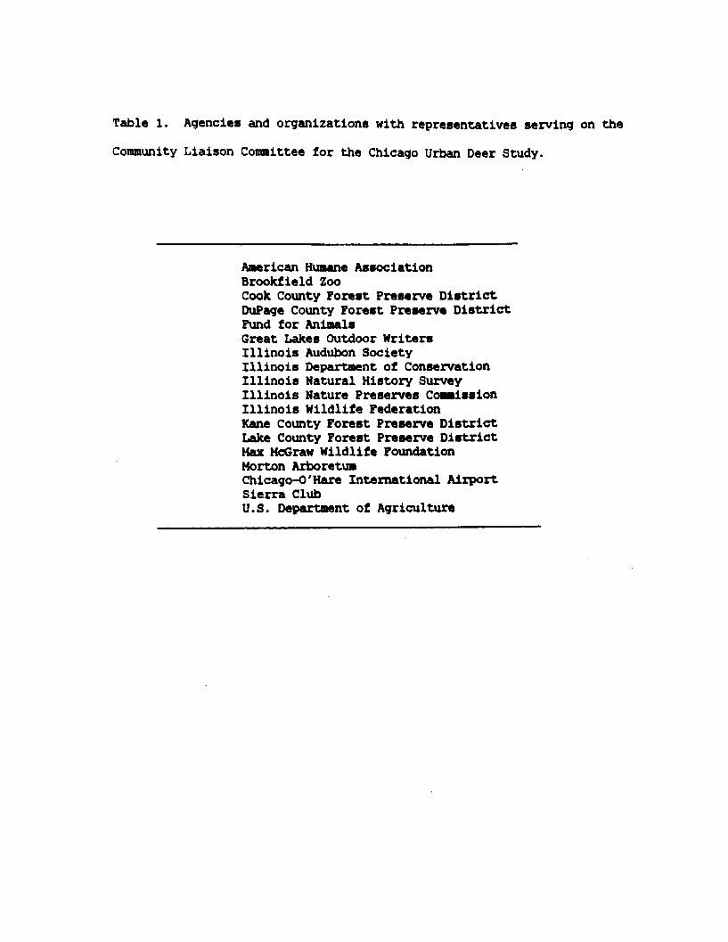
Table 1. Agencies and organizations with representatives serving on the
Community Liaison Committee for the Chicago Urban Deer Study.
American Humane AssociationBrookfield ZooCook County Forest Preserve DistrictDuPage County Forest Preserve DistrictFund for AnimalsGreat Lakes Outdoor WritersIllinois Audubon SocietyIllinois Department of ConservationIllinois Natural History SurveyIllinois Nature Preserves ComissionIllinois Wildlife FederationKane County Forest Preserve DistrictLake County Forest Preserve DistrictMax McGraw Wildlife FoundationMorton ArboretumChicago-O'Hare International AirportSierra ClubU.S. Department of Agriculture

Table 2. Outline of deer reduction plan for the Ned Brown Preserve, Cook County,
Illinois.
I. Problem statement - The number of white-tailed deer in the Ned BrownPreserve has exceeded the ability of the vegetaion to support them on asustained basis. Deer, through browsing, have substantially decreasedforest regeneration and have severely reduced understory vegetation. Thedeer herd (1985) is a phase of "destructive overshoot"--a situation wheredeer have impacted not only palatable plants but also many of the lesspalatable species. Such conditions are not compatible with maintainingand preserving the diverse array of plant and small animal species thatare indigenous to this site. Chronic malnutrition among Ned Brown deer isapparent and the frequency of deer-vehicle accidents reported on adjacentroads is high.
II. Objectives
A. To reduce deer-browsing pressure to a level that enables theregeneration of forest trees and understory plant species in theBusse Woods Nature Preserve and adjacent areas of the Ned BrownPreserve.
Evaluation: Vegetation measurements (XX)
B. To significantly reduce the number of reported deer-vehicleaccidents on roads adjacent to Ned Brown.
Evaluations Monitor frequency of deer-vehicle accidents on statenumbered highways adjacent to Ned Brown.
C. To significantly improve average physical condition of the deerherd.
Evaluations Postaortem examinations (condition indices, physicalmeasurements, and reproductive performance)
III. Decision Rules Deer will be removed from the Ned Brown Preserve if deerdensity exceeds 8 deer/km2 of deer habitat.
Evaluations Helicopter counts of deer during winter.

Table 3. Outline of key elements of the O'Hare Airport deer reduction plan.
Problem statement: The mission of Chicago-O'Hare International Airport is toprovide safe and efficient air transportation facilities and services.Undeveloped airport property near active runways provides habitat thatsupports relatively large numbers of white-tailed deer. These deer rangefreely and are observed near active runways causing immediate danger toaircraft in transition. Presence of deer on O'Hare property is incompatiblewith airport mission safety. Live-trapping by O'Hare over 4 years wasineffective. Implementation of more effective methods of herd reduction arewarranted.
Program qoal: To reduce probability of deer-aircraft collisions and otherdeer-runway incidents to an acceptable level as defined by O'Hare AviationSafety Department.
Objectives,
1) To define the maximum number of deer that O'Hare will accept onairport property. This maximum number will be used as adecision rule above which reduction will be implemented.
2) To select a deer management strategy from long and short term optionsthat recognizes the need for periodic, perhaps annual, control efforts.
3) To provide the economic, logistic, and political support needed toimplement deer management during autumn 1987.
4) To reduce deer numbers to a level below the defined decision rulethreshold before 1 April 1988.
5) To provide regular and effective evaluations of deer numbers, and tomaintain numbers at or below the specified decision rule indefinitely.
6) To minimize negative publicity and intra-agency controversy.
Decision rule: INHS identified 4 levels of deer abundance including no maximumpopulation size, moderate to high residual population (<20 deer), low residualpopulation (510 deer), and remove all deer. O'Hare selected a low residualpopulation because it was unlikely that all deer could be removed from thesite.
Methods selected from short- and long-term management options
1) Live-trapping and translocation2) Live-trapping and euthanasia3) Sharpshooting from elevated stands near baited sites
Program evaluation: Helicopter count during winter

Table 4. Summary of Lake County Forest Preserve District plan for deer
management at Ryerson Conservation Area.
I. Problem statement- The primary site objectives are to preserve, protect,and maintain the biological diversity of existing natural communities onboth a short-term basis. Browsing by deer has caused a rudimentary browseline and an apparent decline in key indicator spring ephemeral plantscreating a visible change in the forest understory. Deer appear inexcellent condition and to be increasing in abundance. The number of deeron Ryerson must be regulated if sensitive components (i.e., most palatableplant species and animals dependent on those species) within existingnatural communities are to maintained. The Lake County Forest PreserveDistrict has no operational plan for management of deer at Ryerson.
II. Program goal - to develop a deer management program that is effective,regards human safety with priority, provides humane treatment of deer,enhances public education, and minimizes the total number of deer killed,handled, or treated over time.
III. Program objectives
A. To develop and implement a short-term strategy that will reduce thetotal number of deer on Ryerson Conservation Area to 12 animals(i.e., 15 deer/mile 2) by 15 March 1989.
B. To develop and implement a long-term strategy that will maintain deernumbers at a level that minimizes negative effects to key indicatorplant species such as white trillium (Trillium qrandiflora).
C. To promote opportunities for community education, informationexchange, and public involvement in deer management activitiesthrough organized volunteer participation.
IV. Site description and resource inventoriesA. Draft master plan (Nuzzo 1988)
1. Description of 9 natural communities2. Description of rare and endangered species
B. Illinois Natural Heritage database records
V. Documentation of adverse effects on resources
A. Qualitative assessments1. Current and historic photographs of site vegetation2. Department of Conservation evaluation of botanical risks
B. Quantitative assessments1. Aerial counts of deer2. Preliminary analysis of plant density, percent cover, and
frequency of occurence within the deer exclosure/control plot
VI. Review of alternate methods of deer control
A. Outline of alternative methods of deer controlB. Citations of literature reviewed
cont.
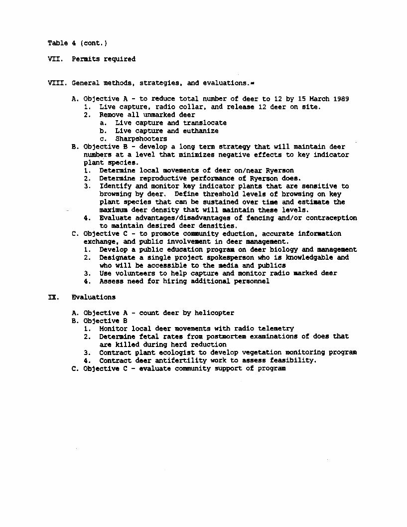
Table 4 (cont.)
VII. Permits required
VIII. General methods, strategies, and evaluations.=
A. Objective A - to reduce total number of deer to 12 by 15 March 19891. Live capture, radio collar, and release 12 deer on site.2. Remove all unmarked deer
a. Live capture and translocateb. Live capture and euthanizec. Sharpshooters
B. Objective B - develop a long term strategy that will maintain deernumbers at a level that minimizes negative effects to key indicatorplant species.1. Determine local movements of deer on/near Ryerson2. Determine reproductive performance of Ryerson does.3. Identify and monitor key indicator plants that are sensitive to
browsing by deer. Define threshold levels of browsing on keyplant species that can be sustained over time and estimate themaximum deer density that will maintain these levels.
4. Evaluate advantages/disadvantages of fencing and/or contraceptionto maintain desired deer densities.
C. Objective C - to promote community eduction, accurate informationexchange, and public involvement in deer management.1. Develop a public education program on deer biology and management2. Designate a single project spokesperson who is knowledgable and
who will be accessible to the media and publics3. Use volunteers to help capture and monitor radio marked deer4. Assess need for hiring additional personnel
IX. Evaluations
A. Objective A - count deer by helicopterB. Objective B
1. Monitor local deer movements with radio telemetry2. Determine fetal rates from postmortem examinations of does that
are killed during herd reduction3. Contract plant ecologist to develop vegetation monitoring program4. Contract deer antifertility work to assess feasibility.
C. Objective C - evaluate community support of program

Table 5. Minimum winter density of white-tailed deer on selected forest
preserves in Lake County, Illinois.
No. of deer DensityLocation Area (km2) counted (Deer/km2)
Columbian Gardens 0.91 17 19Ryerson Cons. Area 2.23 52 23Daniel Wright Wds. 2.54 55 22
& Lloyds Wds.MacArthur Wds. & 2.05 37 18
N. of MacArthurOld School 2.10 40 19Wilmot Wds. 4.97 44 9Riverhill 1.68 26 15Gurnee Wds. 3.24 10 3Wadsworth 4.53 25 6Van Patten Wds. 4.38 30 7Cuba Marsh 2.25 5 2Countryside Golf C. 1.99 0 0Lakewood 5.62 44 8Gavin Bog & N.P. 2.23 15 7Spring Bluff 1.01 6 6Lyons Wds. 1.09 22 20Greenbelt 2.15 1 0Gander Mt. 1.24 22 18
aCounts made by 2 observers in Bell
31 Dec 87 and 8 Jan 88.Long Ranger helicopter on

Table 6. Minimum winter density of white-tailed deer on selected foresta,b,c
preserves in DuPage County, Illinois.
No. of deer counted
Area DensityLocation (km2) 1985 1987 1988 (deer/km2)
Blackwell 4.53 14 13 12 3Burlington Park 0.21 0 0 0 0Churchill Wds. 0.98 0 2 2 0 - 2Greene Valley 5.83 29 21 19 3 - 5Herrick/Danada 6.24 6 19 17 1 - 3Hidden Lake 1.58 11 13 31 7 - 20McDowell Grove 1.68 0 1 17 0 - 10Pratt's Wayne Wds. 5.18 2 11 15 0 - 3Springbrook 7.20 0 0 9 0 - 1Timber Ridge 2.46 19 19 28 8 - 11Waterfall Glen 9.84 71 217 221 7 - 22W. Branch DuPage River 7.04 23 22 13 2 - 4West DuPage 1.89 3 0 2 0 - 2Winfield Mounds 1.37 4 6 3 2 - 4
aCounts made by 2 observers in
and 16 Feb 85.bCounts made by 2 observers inJan 87 and 22 Jan 87.cCounts made by 2 observers in
Jan 88 and 27 Jan 88.
fixed-wing Cessna 172 on 30 Jan 85
Bell Long Ranger helicopter on 21
Bell Long Ranger helicopter on 7

Table 7. Minimum winter density of white-tailed deer on selected forest
preserves in southern Cook County, Illinois.
No. of deer counted
Area a b c DensityLocation (km2) 1983 1985 1988 (deer/km2)
Sag Valley DivisionE. Willow Rd. 7.49 41 48 5 - 6W. Willow Rd. 9.30 71 119 8 - 13Tampier Lake 4.87 24 33 5 - 7McGinnis Slough 4.40 22 22 5
Palos DivisionW. Willow Rd. 12.46 78 60 125 5 - 10E. Willow Rd. 12.38 113 273 247 9 - 22Black Partridge Wds. 1.37 0 0 0
Salt Creek DivisionW. Rt 45/S. 31st 4.45 13 17 3 - 422nd to 31st 2.05 11 4 2 - 5Zoo & DesPlaines R. 4.45 0 0 0Lake Ida 2.38 23 13 5 - 10
Calumet DivisionEggers Grove 0.70 0 0 0Burnham Wds. Golf C. 1.24 0 0 0Beaubien Wds. 1.01 0 0 0Calumet-Sag Channel 3.00 3 0 0 - 1Dan Ryan Wds. 0.85 0 0 0Calumet Playfield 0.80 0 0 0Sand Ridge Nat. Cent. 2.10 0 1 0
Tinley Creek DivisionN. of 151st 13.49 19 31 1 - 2104th Ave. property 3.24 9 6 2 - 3S. of 151st 20.88 34 42 2
Thorn Creek DivisionN. Glenwood-Dyer 11.66 35 33 3S. Glenwood/N.Linc. 3.57 13 17 4 - 5S. Lincoln Highway 5.67 25 18 3 - 4Plum Creek 4.38 13 23 3 - 5
aCounts made by 2 observers in fixed-wing Cessna 1/2 on 30-31 Dec 1983 and 4
Jan 1984.b
Counts made by 2 observers in fixed-wing Cessna 1/2 on 15 Jan, 28-i0 Jan,and 19 Feb 1985.c
Counts made by 2 observers in Bell Long Ranger helicopter on 29 Jan 1988.

Table 8. Minimum winter density of white-tailed deer on selected forest
preserves in southern Cook County, Illinois.
No. of deer counted
Area a b c d e f g DensityLocation (km2) 1983 1985A 19858 1986 1987A 1987B 1988B (deer/km2)
New DivisionPoplar Ck. W. SuttonPoplar Ck. E. SuttonSpring Lake N. DundeeSpring Lake S. DundeeCrabtree N. C.Deer GrovePaul DouglasBakers Lake
DesPlaines RiverMadison - NorthNorth - BelmontBelmont - Irving Pk.Irving Pk. - LawrenceLawrence - 1/901/90- DevonDevoh - TouhyTouhy - OaktonOakton - GolfGolf - CentralCentral - LakeLake - PalatinePalatine - DundeeDundee - Lake/Cook
Skokie DivisionS. OaktonOakton - GolfGolf - WillowWillow - DundeeDundee - Lake/CookWest of 1/94
Ned Brown PreserveN. Rt. 72S. Rt. 72
5.0211.018.916.794.696.795.181.14
1.421.092.381.941.860.850.880.701.270.832.902.313.731.84
2312274037
8200
231556323422300
8034213816131921305360
11973
28130248058
2.90 1 74.43 6 8 1310.98 25 8 128.78 74 36 544.95 20 8 155.41 35 15 46
6.89 258 167 2077.95 35 44 46
40602330698
2125
10653
12053
48
46712169
20
2129357510132891295147
8426921042
154 8536 33
Fixed-wing Cesna 172 on 12/27/83, 12/30/83, 12/31/83, & 1/13/84
Fixed-wing Cessna 172 on 1/05/85, 1/27/85. and 1/30/85
Bell Long Ranger helicopter on 1/21/85 and 1/22/85
Bell Long Ranger helicopter on 2/11/86
Bell Long Ranger helicopter on 3/16/87
Bell Long Ranger helicopter on 1/03/88. 1/05/88. and 1/06/88
515 -3 -7 -
.X -
4 -0
I -09 -
11 -16 -
7 -6 -
11 -10 -30 -18 -10 -14 -26 -
0 -1 -1 -4 -1 -3 -
7 -4 -
66836
6
251520191527173645263240
335
10413
377
348669
61152645
61
4756
a
b
C
d
e
£
5841

Table 9. Reproductive performance of does from 5 locations within the
Chicago metropolitan area, 1984-85.
Female age No. of doesclass by No. of doesarea examined Fetuses/N
(N) Aparous Singleton Twin Triplet
Fawn
Ned BrownDes PlainesPalosNorthwest CookNon-Cook
15167
1523
1516479
0036
10
0 00024
000.430.670.78
Yearling
Ned BrownDes PlainesPalosNorthwest CookNon-Cook
Adult
Ned BrownDes PlainesPalosNorthwest CookNon-Cook
513229
31102
2122655
110100
118110
01000
912522
0.601.150.502.001.56
00023
1.381.451.832.202.60

Table 10. Cause specific mortality and survival of fawn white-tailed deer
captured, marked, and released on the Ned Brown Preserve, Cook County, Illinois.
Cause of Death
Interval No. ofInterval Days Survival Survival 95% CI loadkill Collected Unknom
Days late
Male
Dec 83-Jun 84 181 2,681 0.873 0.722*1.000 0.000 0.000 0.127 (1)
Dec 84-Jun 85 180 997 0.694 0.419-1.000 0.000 0.153 (1) 0.153 (1)
Fesale
Dec 83-Nay 84 181 864 0.809 0.534-1.000 0.000 0.191 (1) 0.000
Dec 84-Jun 85 180 820 0.801 0.518-1.000 0.000 0.000 0.200 (1)

Table 11. Cause specific mortality and survival of yearling white-tailed deer
captured, marked, and released on the Ned Brown Preserve, Cook County, Illinois.
Cause of DeathNo. of
Interval SurvivalInterval Days Days Survival 95% CI Roadklill Collected Unknon
Male
Jan 84-Nay 84 152 486 1,000 0.000 0.000 0.000
Jun 84-*Nov 84 183 2,944 0.830 0.672-1.000 0.170 (3) 0.000 0.000
Dec 84-Nay 85 182 2,795 0.937 0.824-1.000 0.063 (1) 0.000 0.000
Jun 85-Nov 85 183 1,065 0.840 0.598-1.000 0.000 0.159 (1) 0.000
Dec 85*Apr 86 151 199 0.218 0.026-1.000 0.000 0.782 (2) 0.000
Female
Jan 84-*ay 84 152 117 0.271 0.021-1.000 0.000 0.000 0.729 (1)
Jun 84-Mov 84 183 915 1.000 0.000 0.300 0.000
Dec 84-*ay 85 182 1,132 0.851 0.621-1.000 0.000 0.000 0.149 (1)
Jaun 85Iov 85 183 1,139 1.000 0.000 0.000 0.000
Dec i5-Nay 86 182 738 0.476 0.206-1.000 0.175 (1) 0.349 (2) 0.000

Table 12. Cause specific mortality and survival of adult white-tailed deer
captured, marked, and released on the Ned Brown Preserve, Cook County, Illinois.V
Cause of DeathNo. of
Interval SurvivalInterval Days Days Survival 95% CI Roadkill Collected Unknown
Male
Dec 83-Nay
Jun 84-Nov
Dec 84-May
Jun 85-Nov
Dec 85-Kay
Jun 86-Nov
94
84
85
85
86
86
183
183
182
183
182
183
972
1,768
1,768
3,413
1,600
1,001
0.828
0.901
0.734
0.687
0.634
0.694
0.572-1.000
0.736-1.000
0.517-1.000
0.520-0.907
0.406-0.990
0.417-1.000
0.172
0.098
0.256
0.224
0.091
0.153
(1)
(1)
(3)
(5)
(1)
(1)
0.000
0.000
0.000
0.000
0.183
0.153
(2)
(1)
0.000
0.000
0.000
0.089 (2)
0.091 (1)
0.000
Fesale
Dec 83-May 84
Jun 84-Nov 84
Dec 84-May 85
Jun 85-Nov 85
Dec 5-Kay 86
Jun 86-Ilo 86
183
183
182
183
182
193
2,055
2,667
2,374
3,328
2,427
1,704
0.765
1.000
0.681
0.848
0.591
0.471
0.565-1.000 0.000
0.000
0.487-0.953 0.191 (3)
0.703-1.000 0.152 (3)
0.400-0.872 0.000
0.269-0.822 0.076 (1)
0.000
0.000
0.000
0.000
0.409
0.454
0.235 (3)
0.000
0.127 (1)
0.000
0.000
0.000
(7)
6)
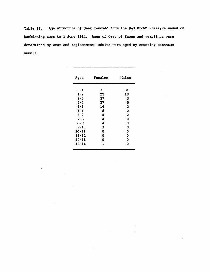
Table 13. Age structure of deer removed from the Ned Brown Preserve based on
backdating ages to 1 June 1984. Ages of deer of fawns and yearlings were
determined by wear and replacement; adults were aged by counting cementum
annuli.
Ages Females Males
0-1 31 311-2 22 192-3 37 33-4 27 84-5 14 25-6 8 06-7 4 27-8 4 08-9 4 09-10 2 0
10-11 0 - 011-12 0 012-13 0 013-14 1 0
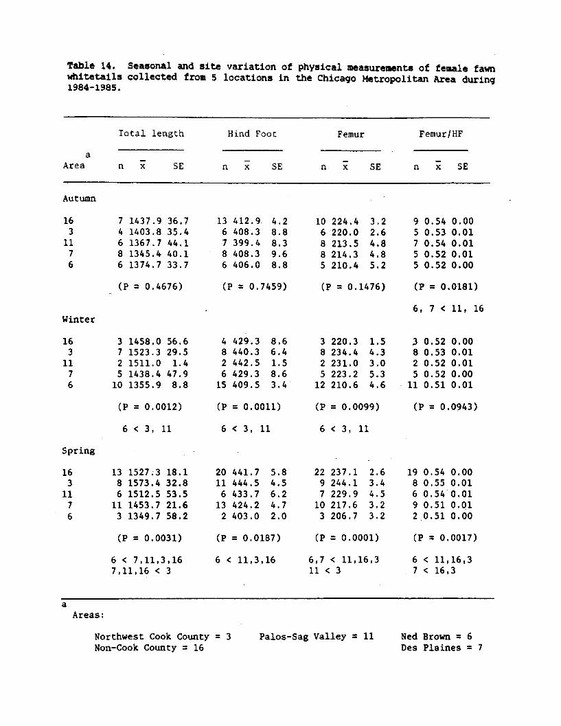
Table 14. Seasonal and site variation of physical measurements of female fawnwhitetails collected from 5 locations in the Chicago Metropolitan Area during1984-1985.
Total length Hind Foot Femur Femur/HF
aArea n x SE n x SE n x SE n x SE
Autumn
163
1176
1437.91403.81367.71345.41374.7
36.735.444.140.133.7
136786
412.9.408.3399.4408.3406.0
4.28.88.39.68.8
106885
224.4220.0213.5214.3210.4
3.22.64.84.85.2
95755
0.540.530.540.520.52
0.000.010.010.010.00
(P = 0.4676)
372510
1458.01523.31511.01438.41355.9
56.629.51.4
47.98.8
(P = 0.7459)
482615
(P = 0.0012)
6 < 3, 11
1386
113
1527.31573.41512.51453.71349.7
429.3440.3442.5429.3409.5
8.66.41.58.63.4
(P = 0.1476)
382512
(P = 0.0011)
6 < 3, 11
18.132.853.521.658.2
20116132
441.7444.5433.7424.2403.0
220.3234.4231.0223.2210.6
1.54.33.05.34.6
(P = 0.0181)
6, 7 < 11, 16
3825
11
(P = 0.0099)
0.520.530.520.520.51
0.000.010.010.000.01
(P = 0.0943)
6 < 3, 11
5.84.56.24.72.0
2297
103
237.1244.1229.9217.6206.7
2.63.44.53.23.2
198692
0.540.550.540.510.51
0.000.010.010.010.00
(P = 0.0031)
6 < 7,11,3,167,11,16 < 3
(P = 0.0187)
6 < 11,3,16
(P = 0.0001)
6,7 < 11,16,311 < 3
(P = 0.0017)
6 < 11,16,37 < 16,3
Northwest Cook County = 3Non-Cook County = 16
Palos-Sag Valley = 11 Ned Brown = 6Des Plaines = 7
Winter
163
1176
Spring
163
1176
Areas:

Table 15. Seasonal and site variation of measurements of the condition of femalefawn whitetails collected from 5 locations in the Chicago Metropolitan Areaduring 1984-1985.
Whole Body Kistner Kidney FatGirth (mm) Weight (kg) Evaluation Index
aArea n x SE n x SE n x SE n x SE
Autumn
163
1176
46476
740.8743.8727.8729.7734.5
29.319.919.529.09.9-
40.237.436.432.334.2
1.93.43.63.22.3
78696
65.760.059.247.262.5
3.710.45.17.-55.0
126796
1.071.091.320.971.51
0.150.390.320.230.17
(P = 0.9862)
792.0813.3803.0771.3684.8
22.021.92.0
22.313.3
(P = 0.0002)
6 < 7,11,3,16
771.2787.5682.3707.8686.0
10.023.314.612.213.2
26239
(P = 0.2804)
34.241.139.236.724.8
2.53.10.21.62.0
(P = 0.0009)
6 < 3
158493
40.9 1.544.8 3.334.1 4.128.2 1.925.9 0.8
20.96123
28258
(P = 0.2180)
30.063.835.043.013.8
0.07.55.07.27.Q,
(P = 0.0008)
6 < 3
33.040.626.717.913.3
3.84.89.33.78.3
372610
(P = 0.5688)
0.261.470.580.610.31
0.060.260.210.110.10
(P = 0.0002)
6, 16 < 3
1810693
0.390.310.270.150.11
0.140.060.080.020.03
(P = 0.0001)
11,6,7 < 16,3
(P = 0.0001)
6, 7 < 3, 16
(P = 0.0144) (P = 0.6099)
6 < 3
Northwest Cook County = 3Non-Cook County = 16
Palos-Sag Valley = 11 Ned Brown = 6Des Plaines = 7
Winter.
163
1176
2723
10
Spring
163
1176
116483
Areas:

Table 16. Seasonal and site variation of physical measurements of male fawnwhitetails collected from 5 locations in the Chicago Metropolitan Area during1984-1985.
Total length Hind Foot Femur Femur/HF
Area n x SE n x SE n x SE n x SEArea n x SE n x SE n x SE n x SE
Autumn
163
1176
87895
1486.01444.01405.61431.91405.8
21.325.723.123.035.1
1289
115
440.4430.5412.8429.4430.4
5.35.68.26.19.0
1189
115
233.5234.0218.1225.9219.4
3.62.74.13.16.5
1087
105
0.540.540.530.530.51
0.000.000.000.010.01
(P = 0.1565) (P = 0.0605) (P = 0.0127) (P = 0.0324)
6 < 3
452
1010
1606.31558.21601.51487.01437.3
13.029.136.520.630.7
5941316
(P = 0.0024)
444.0453.2448.5432.4428.3
11.55.86.24.95.3
6831414
(P = 0.0278)
6 < 11,16
237.3239.5230.0223.2218.6
7.04.05.83.32.6
(P = 0.0014)
5831212
0.530.530.510.520.51
0.010.010.010.000.01
(P = 0.1783)
6 < 3
22 1636.5 13.763174
1524.71534.31513.41517.3
109.381.628.368.3
24 459.9 12.174214
454.1458.0447.4454.5
6.917.74.8
13.0
(P = 0.0377)
6 < 11,16
(P = 0.9082) (P = 0.0026) (P = 0.7528)
6 < 16
Northwest Cook County = 3Non-Cook County = 16
Palos-Sag Valley = 11 Ned Brown = 6Des Plaines = 7
Winter
163
1176
Spring
163
1176
2865205
252.6242.5240.4238.3228.8
2.15.86.72.7
15.0
236419
4
0.570.530.530.530.53
0.040.010.010.000.01
Areas:

Table 17. Seasonal and site variation of the condition of male fawn whitetailscollected from 5 locations in the Chicago Hetropolitan Area during 1984-1985.
Whole Body Kistner Kidney FatGirth (mm) Weight (kg) Evaluation Index
aArea n x SE n x SE n x SE n x SE
Autumn
163
1176
800.0844.4795.2790.8756.2
19.921.717.918.126.5
41.845.036.841.036.8
1.31.93.31.72.5
87695
64.462.958.365.669.0
2.05.25.43.84.8
129885
1.161.071.461.501.63
0.230.190.260.260.57
(P = 0.0899)
341812
842.3826.8783.0752.1718.3
19.123.8
21.812.7
(P = 0.0017)
137313
4
847.1811.1800.3756.1795.3
(P = 0.0657)
452810
47.347.545.436.028.9
1.22.70.92.31.4
(P = 0.0001)
6 < 11,16,37 < 16,3
10.213.835.014.348.2
2063174
50.843.842.338.739.1
1.42.85.11.97.2
(P = 0.5716)
672910
50.061.462.527.811.5
8.56.017.56.63.4
(P = 0.0001)
6 < 16, 3 117 < 3, 11
2263184
32.325.821.722.218.7
2.96.46.02.57.2
(P = 0.5921)
8731310
0.861.311.520.460.28
0.210.280.320.110.05
(P = 0.0001)
6, 7 < 3, 11
237315
2
0.190.150.160.170.11
0.020.020.050.020.03
(P = 0.0021) (P = 0.0005) (P = 0.0969) (P = 0.7227)
7 < 16
Areas:
Northwest Cook County = 3Non-Cook County = 16
Palos-Sag Valley = 11 Ned Brown = 6Des Plaines = 7
Winter
163
1176
Spring
163
1176

Table 18. Seasonal and site variation of physical measurements of femaleyearling whitetails collected from 5 locations in the Chicago Metropolitan Areaduring 1984-1985.
Total length Hind Foot Femur Femur/HF
aArea n x SE n x SE n x SE n x SE
Summer
16311
76
122463
1602.51659.51621.51598.51476.7
14.721.511.616.76.1
142553
458.7463.5437.4464.6444.7
4.114.55.99.56.5
132562
252.1258.0249.4244.5240.0
1.95.02.83.08.0
122552
0.550.560.570.530.55
00.030.010.010.01
(P = 0.0006)6 < 3,7,11,16
(P = 0.0640) (P = 0.0507)6 < 3
(P = 0.0325)
1581.0 31.71470.01544.0
1642.3 91.5
92123
446.4 9.7448.5 28.5471.0447.0 5.0463.3 10.5
(P = 0.5858) (P = 0.8328) (P = 0.4375) (P = 0.5812)
1575.5 18.51660.01612.01542.0 21.01518.0
21242
467.0 1.0462.0474.0 2.0458.5 2.7462.0 5.0
(P = 0.1726)
11 1575.1 19.17 1568.3 35.41 1494.06 1548.2 38.75 1525.8 34.7
(P = 0.7125)
(P = 0.0824)
137276
454.6443.4445.0458.4454.7
4.27.1
21.010.96.3
(P = 0.6367)
(P = 0.7250)
116165
244.4246.5247.0249.0231.0
(P = 0.7403)
3.84.3
4.61.9
116165
(P = 0.1020)
0.54 0.010.55 0.020.530.54 0.010.51 0.01
(P = 0.0367)
Areas:Northwest Cook County = 3Non-Cook County = 16
Palos-Sag Valley = 11 Ned Brown = 6Des Plaines = 7
Autumn
16311
76
Winter
243-.8256.0258.0250.0316.3
6.0
5.00
74.3
8I123
0.55 0.010.540.560.56 0.010.68 0.14
163
1176
21233
253.5250.0251.5245.7240.7
0.54 0.014.5
5.57.47.2
20232
Spring
163
1176
0.530.540.52
0.010.010.02
a

Table 19.whitetails1984-1985.
Seasonal and site variation in the condition of female yearlingcollected from 5 locations in the Chicago Metropolitan Area during
Whole Body Kistner Kidney FatGirth (mm) Weight (kg) Evaluation Index
aArea n x SE n x SE n x SE n x SE
Summer
814.4 15.1849.0 61.0
854.6 26.1774.0 11.0
112443
49.349.251.050.345.7
2.75.24.94.70.8
141563
50.630.062.064.246.7
4.8
5.66.24.4
0.400.140.600.890.28
0.14
0.260.260.10
(P = 0.2669)
799.8850.0906.0886.0920.3
52.9
23.9
(P = 0.9420)
71123
56.244.952.655.854.6
1.8 821
0.5 26.7 3
(P = 0.1607)
74.477.580.067.570.0
2.97.5
2.57.6
(P = 0.2786)
91I123
1.233.021.561.441.85
0.24
0.730.39
(P = 0.5674)Winter
898.0 44.0926.0904.0 6.0859.0
(P = 0.6307)
2 54.7 8.80231
56.054.940.4
2.03.5
(P = 0.7038)
11211
70.075.085.070.085.0
5.0
(P = 0.2630)
2I242
1.77 0.800.972.77 0.811.33 0.271.53 0.64
(P = 0.7694)
808.4801.2803.0797.3785.6
8.317.5
29.428.6
(P = 0.9446)
(P = 0.4548)
77166
50.549.944.050.240.3
4.7 113.6 7
13.1 62.1 6
(P = 0.2758)
(P = 0.5519)
54.150.735.045.824.2
5.46.4
15.53.06.0
(P = 0.3971)
117154
(P = 0.0117)
0.330.450.150.240.14
0.050.17
0.070.05
(P = 0.3666)
Areas:Northwest Cook County = 3Non-Cook County = 16
Palos-Sag Valley = 11 Ned Brown = 6Des Plaines = 7
163
1176
Autumn
16311
76
163
1176
Spring
16311
76

Table 20.whitetails1984-1985.
Seasonal and site variation in the condition of male yearlingcollected from 5 locations in the Chicago Metropolitan Area during
Whole Body Kistner Kidney FatGirth (mm) Weight (kg) Evaluation Index
aArea n x SE n x SE n x SE n x SE
Summer
163
1176
917.0879.4980.0899.0905.0
38.023.0
12.0
67.261.962.660.5
3.7 56.1 5
13.0 3
1
63.054.065.056.755.0
5.48.9
6.7
23122
0.410.240.550.340.43
0.180.05
0.180.09
(P = 0.4230)
1000.01004.0893.0918.0856.7
27.827.19.0
89.050.6
(P = 0.8252)
76.279.571.266.667.9
(P = 0.8870)
2.56.43.34.26.2
71.778.876.074.082.5
6.36.34.34.67.5
(P = 0.6269)
1285
114
1.211.271.331.361.59
0.180.270.410.240.51
(P 0.602)
920.0
834.7
(P 0r310)
6 < 3
857.8883.7904.0897.0823.5
7.7
(P = 0.1977)
1 56.21 64.002 43.1 5.9
(P = 0.4230)
(P = 0.7749)
1 50.01 75.0
(P = 0.9373)
11113
02 27.5 27.5
(P = 0.7082)
0.391.090.810.560.19 0.05
(P = 0.0315)
6 < 3
14.625.8
75.07.5
114122
53.154.465.851.551.0
1.1 144.2 4
19.8 30.2 2
43.637.545.031.740.0
4.86.0
23.711.75.0
154143
0.210.210.240.440.22
0.030.03
0.220.06
(P = 0.5416) (P = 0.3392) (P = 0.8302) (P = 0.3129)
Areas:Northwest Cook County = 3Non-Cook County = 16
Palos-Sag Valley = 11 Ned Brown = 6Des Plaines = 7
Autumn
163
1176
65223
Winter
163
1176
01003
Spring
163
1176
103122
a

Table 21. Seasonal and sitewhitetails collected from 51984-1985.
variation of physical measurements of male yearlinglocations in the Chicago Metropolitan Area during
Total length Hind Foot Femur Femur/HF
aArea n x SE n x SE n x SE n x SE
Summer
1706.0 26.61665.2 50.11542.01658.0 47.51747.0
(P = 0.5169)
1749.71750.51686.71699.41644.7
38.138.424.750.155.7
498.2 10.4479.2 15.7481.0469.0 5.6461.0
(P = 0.4906)
147684
489.1482.7476.7472.9474.0
5.45.4
11.35.2
13.9
3 274.3 5.75 270.6 7.21 261.04 256.5 3.92 255.5 13.5
(P = 0.3454)
157674
275.6283.9263.8271.9250.3
1.73.44.03.211.7
0.55 0.010.57 0.010.540.55 0.01
(P = 0.3971)
134564
0.570.580.550.570.53
0.010.010.020.010.01
(P = 0.6211)
1 1744.01 1665.0
(P = 0.4163)
121032 1638.5 33.5
(P = 0.4805)
134232
1632.81659.81821.01710.01627.5
30.731.70
96.39.5
479.0489.0 6.0504.0
476.3 8.3
(P = 0.4047)
164243
482.7486.5480.0483.3440.7
4.56.16.0
12.06.0
(P = 0.0001)6 < 3,7,1611 < 3
1 274.01 263.01 267.002 255.5 1.5
(P = 0.1690)
153234
261.7261.7262.5255.3238.5
2.95.86.58.89.6
(P = 0.0572)6 < 3
11102
0.570.530.53
0.53 0.01
(P = 0.3346)
133233
0.540.540.550.530.55
0.010.020.0100.02
(P = 0.4653) (P = 0.0118)6 < 3,7,11,16
(P = 0.0532) (P = 0.8119)
Areas:Northwest Cook County = 3Non-Cook County = 16
Palos-Sag Valley = 11 Ned Brown = 6Des Plaines = 7
163
1176
45131
Autumn
1631176
96353
Winter
1631176
Spring
163
1176
a

Table 22. Site variation of physical measurements of female whitetails >2 yearsold collected from 5 locations in the Chicago Metropolitan Area.
Total length Hind Foot Femur Femur/HF
aArea n x SE n x SE n x SE n x SE
All Seasons
16 18 1638.1 13.1 22 468.1 3.9 24 255.7 1.5 19 0.55 03 9 1710.8 17.3 13 467.7 6.1 12 255.4 2.7 11 0.55 0.0111 15 1676.3 21.7 16 470.5 6.4 19 251.5 1.8 16 0.54 0.017 52 1650.9 11.8 59 464.3 2.5 63 250.7 1.1 55 0.54 06 30 1644.4 15.1 40 462.2 2.8 39 246.6 2.8 38 0.53 0.01
(P = 0.1390) (P = 0.5666) (P = 0.0123) (P = 0.1275)
6 < 3,16
Areas:Northwest Cook County = 3Non-Cook County = 16
Palos-Sag Valley = 11 Ned Brown = 6Des Plaines = 7
a
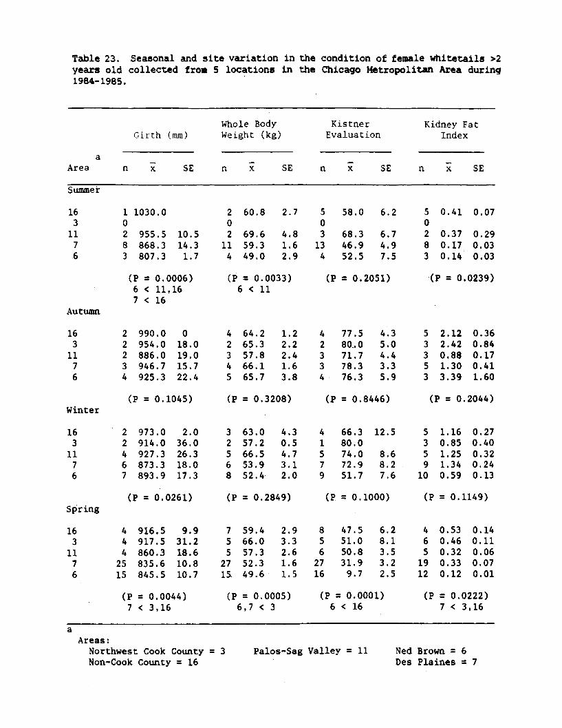
Table 23. Seasonal and site variation in the condition of female whitetails >2years old collected from 5 locations in the Chicago Metropolitan Area during1984-1985.
Whole Body Kistner Kidney FatGirth (mm) Weight (kg) Evaluation Index
aArea n x SE n x SE n x SE n x SE
Summer
1 1030.002 955.58 868.33 807.3
10.514.31.7
(P = 0.0006)6 < 11,167 < 16
990.0954.0886.0946.7925.3
2 60.8 2.702 69.6 4.8
11 59.3 1.64 49.0 2.9
(P = 0.0033)6 < 11
018.019.015.722.4
(P = 0.1045)
973.0914.0927.3873.3893.9
64.265.357.866.165.7
5 58.0 6.2
3134
68.346.952.5
6.74.97.5
(P = 0.2051)
1.22.22.41.63.8
(P = 0.3208)
2.036.026.318.017.3
32568
63.057.266.553.952.4
4.30.54.73.12.0
77.580.. 071.778.376.3
5 0.41 0.0702 0.37 0.298 0.17 0.033 0.14 0.03
(P = 0.0239)
4.35.04.43.35.9
(P = 0.8446)
41579
66.380.074.072.951.7
12.5
8.68.27.6
2.122.420.881.303.39
0.360.840.170.411.60
(P = 0.2044)
5359
10
1.160.851.251.340.59
0.270.400.320.240.13
(P = 0.0261)
916.5917.5860.3835.6845.5
9.931.218.610.810.7
(P = 0.0044)7 < 3,16
(P = 0.2849)
755
2715i
59.466.057.352.349.6
2.93.32.61.61.5
(P = 0.0005)6,7 < 3
8562716
(P = 0.1000)
47.551.050.831.99.7
6.28.13.53.22.5
(P = 0.1149)
4651912
(P = 0.0001)6 < 16
0.530.460.320.330.12
0.140.110.060.070.01
(P = 0.0222)7 < 3,16
Areas:Northwest Cook County = 3Non-Cook County = 16
Palos-Sag Valley = 11 Ned Brown = 6Des Plaines = 7
163
1176
Autumn
1631176
Winter
22234
1631176
Spring
163
1176
4442515
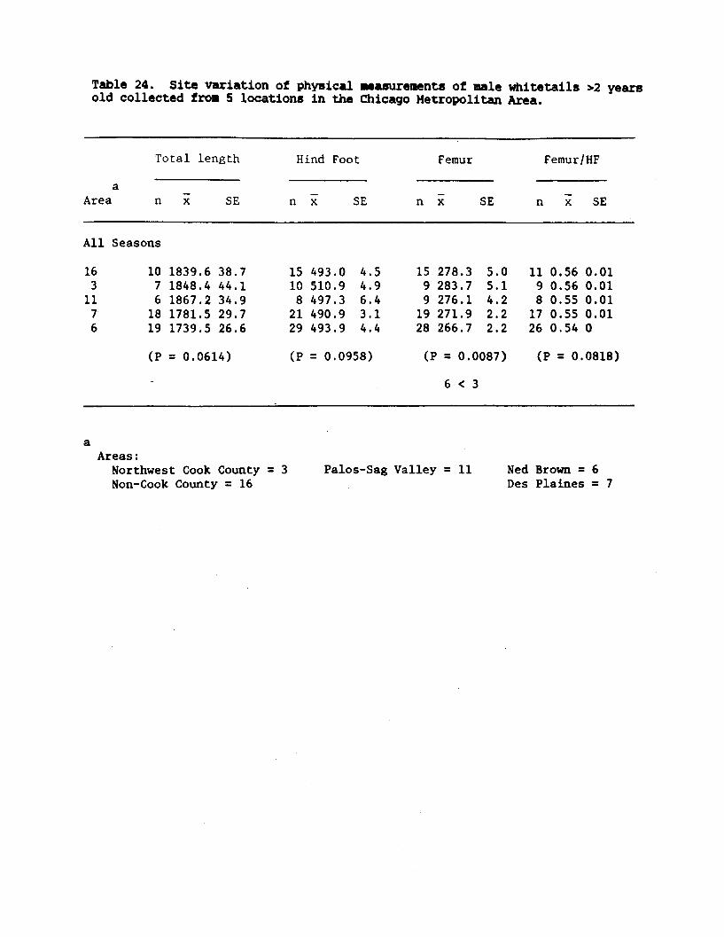
Table 24. Site variation of physical measurements of male whitetails >2 yearsold collected from 5 locations in the Chicago Metropolitan Area.
Total length Hind Foot Femur Femur/HF
aArea n x SE n x SE n x SE n x SE
All Seasons
16 10 1839.6 38.7 15 493.0 4.5 15 278.3 5.0 11 0.56 0.013 7 1848.4 44.1 10 510.9 4.9 9 283.7 5.1 9 0.56 0.0111 6 1867.2 34.9 8 497.3 6.4 9 276.1 4.2 8 0.55 0.017 18 1781.5 29.7 21 490.9 3.1 19 271.9 2.2 17 0.55 0.016 19 1739.5 26.6 29 493.9 4.4 28 266.7 2.2 26 0.54 0
(P = 0.0614) (P = 0.0958) (P = 0.0087) (P = 0.0818)
6 < 3
Areas:Northwest Cook County = 3Non-Cook County = 16
Palos-Sag Valley = 11 Ned Brown = 6Des Plaines = 7

Table 25. Seasonal and site variation in the condition of male whitetails >2years old collected from 5 locations in the Chicago Metropolitan Area during1984-1985.
Whole Body Kistner Kidney FatGirth (mm) Weight (kg) Evaluation Index
aArea n x SE n x SE n x SE n x SE
Summer
002 1092.002 804.5
36.0
55.5
(P = 0.0491)6 < 11
4 1071.8 33.0
1060.01046.4995.0
01 107.52 108.21 112.53 54.4
01
7.9 20
11.3 3
(P = 0.0910)
42165
36.5
(P = 0.8793)
97.6109.880.394.378.3
95.092.5 7.5
55.0 29.3
(P = 0.5912)
10.5 35.4 2
16.4 55.1 5
(P = 0.1617)
73.385.080.068.070.0
16.75.0
11.86.7
(P = 0.8997)
01102
1.601.54
0.71 0.15
(P = 0.2366)
63165
1.381.621.141.741.95
0.380.60
0.560.50
(P = 0.9205)
1108.0981.0 54.9
1010.0927.5 32.5939.8 20.5
(P = 0.2389)
980.0967.7872.0857.0978.0
16.3
14.190.6
(P = 0.2751)
(P = 0.2868)
42153
80.365.856.751.074.1
(P = 0.4167)
7.9 48.2 3
13.0 6
13.5 4
(P = 0.1033)
48.853.35.0
15.047.5
(P = 0.7163)
10.76.7
0.340.260.170.180.24
6.68.8
(P = 0.0136)
0.060.07
0.040.05
(P = 0.3286)
aAreas:
Northwest Cook County = 3Non-Cook County = 16
Palos-Sag Valley = 11 Ned Brown = 6Des Plaines = 7
163
1176
Autumn
163
1176
Winter
16311
76
1312
11
0212
10
69.689.859.659.7
120.2 1
11.9 44.5 11
Spring
40.040.010.038.815.0
12.012.0
17.65.9
132412
0.520.210.390.590.29
1631176
0.100.090.180.14
13153

0EAJr46. /5
Table 26. Mean densities (stems/a 2) of plants <1 i3 Busse Woods exclosure (BEX)and adjacent control plot (BCP), 1984-89 (N=48 I1m quadrats per plot per yearunless otherwise noted).
SPECIES 1984 (August) 1985 (May) 1986 (April) 1987 May 1988 (May) 1989 (May)3EX BC? 5X 3;P B3E 3C? X 3CP BEXa. BC? E!X 0C?
a) herbaceous species
Alliua canadense 0 0 0.8 17.3 16.7 23.7 ".9 23.4 8.9 16.2 0.4 12.4A. tricoccua 0 1.0 1.6 0.3 0.7 7.8 0.1 0.4 T b 4.0 0.5 4.6Allium sp. 0.1 0 0 0 0 0 0 0 0 0 0 0Aneaone spp. 0.5 0.4 0 0 0 0 0 0 0 0 . 0 0A. quinquefolia 0 0 0 0 T 0 T 0.1 0 0 0 0A. virginiana 0.2 0.5 0 0 0 0 0 0 0 0 0 0Anelonella thalictroides 0 0 T 0 0 0.1 0 0 0 0 0 0Ariseasa dracontius 0 0 0.4 1.5 0 T 0.2 0.2 0.2 0.2 0.2 0.1A. triphyllus 0.2 0.3 3.3 7.8 1.0 3.2 2.1 6.4 1.6 4.1 1.6 4.3Aster spp. 0 0 0.2 T T 0 0.1 0 0.1 T 0 0Cardaiine douglassi 0 0 T 1.4 0 4.4 0 1.6 0 6.5 0 5.1Circaea quadrisulcata 0.9 0.1 0.9 0.2 0.4 0.1 1.8 0.3 2.3 0.8 2.4 0.1Claytonia virginiica 0 0 3.4 0 0.9 3,0 0 0 2.0 0.8 2.0 1.5Coaaelina spp. 0. 0 0.2 0 0 0 0.3 0 0 0 0 0Dentaria laciniata 0 0 0 0.1 0 0.6 0 0.1 0 0.6 0 0.5Erigeron spp. 0 0 0 T 0 0 0 0 0 0 0 0Erythroniua albidus 0 0 50.1 3.4 107.3 21.6 2.8 1.7 85.1 11.3 129.3 8.7Floerekia proserpinacoides 0 0 0 0 0 0 0 T 0 0.6 0 2.1Fragara virginiana 0 T 3 T 0 0 0 0 0 0 0 0Galium spp. 0.1 0.1 0.3 0.5 0 T 0.3 0.1 0.1 0.1 1.0 TGeranius aaculatus T T 0.1 0.8 0 0.7 0 0.6 0 0.3 0 0.2GeuM canadense 0 0 0.4 0.9 0.4 0.3 0.7 0.3 0.7 0.2 1.3 0.3Habernaria viridis 0.2 0 0 0 3 0 0 0 0 0 0 0Hackelia virginiana 0 0 0 0 0 0 0 0 0 0 0.2 0.1Hydrophyliua virginianus 0 0 0 0 0 0 0 0 0 T 0 0Hypericua spp. 0 0.1 0 0 0 0 0 0 0 0 0 0Lactuca spp. 0 0 0 0 0 0 T ? T 0,3 0 TOxalis spp. 0.2 0.2 0.3 0.2 T 0.1 0.2 T 0.2 0.2 T 0.2Phlox divaricata 0 0 0.,3 0.8 0.3 0.2 0.2 0.4 1.0 0 0.2 0.8?odophyllua peltatum 0 0 0 0 0.1 0 0.1 0 0.2 0 0 0Polygonus spp. 0 0 0 T 0 0 0 0 0 0 0 0Prenanthes alba 0 0 0 0 0 0.1 0 0.1 0 0 £ 0Ranunculus spp. 0 0 0.2 0 0.2 T 0.1 0.3 1.1 0.3 0.3 0.3Sailacina raceaosa 0 0.1 0.7 0 0.5 0.3 0.3 T 0.3 0.1 C.1 0.4Solidago spp. 0.2 0.3 0.3 0.1 0.2 0.2 0.1 0.2 0.7 0.2 0.3 0.3Taraxacus officlnale 0 0 0 0 0 0 0 T 0 T T 0Tcvara virginiana 3.0 3.56 6.1 3.9 3.4 0.9 5.6 0,9 4.8 0.6 1.7 0.2Trilliua recurvatut 0 0 3.5 0.5 4.1 1.5 f.% 0.5 8.2 1.7 3.0 1.5Urtica spp. 0 0.5 0 0 0 3 0 0.4 0 3.4 0 0Viola spp. 0.3 V.3 0.3 0.4 T T 0.1 0.2 0.1 C.1 0.4 0.3
Nu.Aer of spe:lesMean densityRelative density (%)
12 15 22 13 18 22 21 25 20 25 20 2211.0 7.5 73.6 40,0 136.4 68.8 25.4 38.3 :17.6 49.9 145.1 44.276.9 56,.5 93.8 47.7 94.7 65.3 86.1 51.6 38.5 48.7 87.7. 51.7
cent.

Table 26. (cont.)
SPECIES 1984 ;August) 1935 (May) 1986 (April) 1987 (May) 1988 (May) 1989 (May)BX BCP BX BCBC? 381 BCP E31 BCP BEla BCP EI BCP
b) woody spe:ies
Acer saccharuu 0.1 T 0.3 3 0.1 T T T 8.1 14.2 0 CCarya spp. T 0 C 0 T 0 T C 0.I 0 T 0Crataegus spp. 3.1 0.1 3.1 0.1 T T 0.1 0 0 T T 0Fraxinus spp. T 0.3 T 0 T T T 0 T 0 1.0 1.5Ostrya virginiana 0 0 T 0 T 0 0.1 0.2 0.2 0.1 0.5 TParthenocissus quinquefolia 0.1 0.1 T T T 0 T 0 7 0 T 0Prunus spp. O 0 0 0 0.2 0 0.2 0 T 0 0 0Quercus spp. T T 0 0 0 T 0 0 0* 0 0 0Rhasnus cathartica 0.3 0.5 0.4 0.2 0.5 0.3 0.3 T 0.1 0.1 0.2 0.3Ribes spp. 0.1 T 0 T 0 0.1 0 0 0 0 0 0Rubus spp. 3 0 0 T 0 0 0 0 0 0 0 0Sailax spp. 0.1 0.1 0.3 T 0.1 T 0.2 T T 0 0 0Tilia aaericana T T 0.1 0.1 0.4 0.2 0.6 0.3 1.8 0.8 0 0Toxicodendron radicans 0.2 0.4 0.5 1.0 0.1 0.1 0.2 0.3 1.2 2.9 0.5 1.5Ulaus spp. 0 0.3 0 2.1 3.6 8.4 T T 0.1 0.3 0.9 0Vitis riparia 0 0 T 0 0 T T 0 0 0 T 0Wcody seedlings (i.e., first year) 3.8 3.7 13.5 13.9
Number of species 11 10 10 9 12 11 13 7 11 7t 10 6Mean density 1.1 1.8 1.6 3.5 5.1 9.3 1.8 0.8 11.5 18.3 18.2 17.1Relative density :%) 7.6 13.4 2.0 4.1 3.5 8.8 6.1 1.1 8.7 17.9 11.0 20.0
c) other species
Sedges (i.e., Carex spp.) 0 0 0.2 34.5 2.0 24.1 1.3 28.4 2.7 28.7 1.1 19.8
3:asses (e.g., Sphencpholh s spp., 1.4 3.4 0 2.4 0.1 1.3 0.3 5.5 0.3 5.3 0,2 4.3Pca spp., and Glycer1a spp.)
Unknowns M.8 0.6 3.1 3.6 0.4 1.9 0.2 1.2 0.7 0.2 0.7 0.2
Nuaber of species 2 2 3 6 3 5 3 2 3 3 2 4Mean density 2.2 4.1 3.2 40.5 2.5 27.3 2.3 35. 3.7 34.2 2.0 24.1Relative density (%) 15.5 30.2 4.1 48.2 1.8 25.9 7.S 47.3 2.3 33.4 1.2 28.2
d) all plants
Nuaber of species 25 27 35 38 33 33 37 35 34 35 33 32Mean density 14.3 13.5 % .4 4.0 144.0 105.3 29.5 74.2 132.9 102.4 65.4 85.4
C:ly 8 pernanent line intercepts were usable due to fallen trees,b 2
Trace amounts of <0.05 stesim ,

Table 27. Mean densities (stems/m2) of plants <1m in Busse Woods exclosure (BEX)and adjacent control plot (BCP), 1984-89 (N=48 la' quadrats per area per yearunless otherwise noted).
1'84 (August) 1985 (May) 1986 (April) 1987 (May) 1988 (May) 1989 (May.a
PLANT TYPE BEX BCP BEX BCP BEX BCP BEX BCP BEI BCP BEX BC?
Herbaceous 13.9 6.6 71.2 22.5 119,1 37.3 17.4 14.6 108.7 29.7 144.2 27.2(11)b (14) (20) (21) (16) (20) (19) (23) (18) (23) (18) (20)
Woody 0.8 1.3 1.3 3.3 4.6 9.0 1.5 0.8 11.4 18.2 18.0 16.8(10) (9) (9) (3) (11) (10) (12) (6) (10) (6) (9) (5)
first-year NR(c) NR MR MR 3.8 8.7 MR NR MI I 13.5 13.9'seedlings'
Exotic Woody 0.3 0.5 0.4 0.2 0.5 0.3 0.3 T (d) 0.I 0.1 0.2 0.3(1) (I 1) ( ) (1} (1) (I) il) (1) (1) (1) (1) (1 )
eOthers 2.3 5.1 5.6 58.0 19.9 27.3 10.3 58.8 12.7 54.5 3.0 41.1
(3) (3) (5) (8) (3) (5) (5) (6) (5) (5) (5) (6)
Total 14.3 13.5 78.4 84.0 144.0 105.3 29.5 74.2 132.9 102.4 165.4 85.4(25) (27) (35) (38) (33) (38) (37) (35) (34) (35) (33) (32)
aOnly 32 peruanent quadrats were usable due to fallen trees.
Nuiber cf species shown in parentheses.
Not Recorded during saipling.
Trace amounts cf <0.05 steis/a2.
The "others" category includes grasses, sedges, Alliu: canadense, and A. tricoccum.

Table 28. Mean densities (stems/a 2) of plants <1m in Busse Nature Preserve
during May 1986-1989; number of species shown in parentheses.
Plant Type 1986 1987 1988 1989
Herbaceous 32.4 (20) 38.5 (24) 32.7 (27) 28.2 (28)
Woody 17.3 (14) 3.7 (15) 5.7 (15) 7.5 (15)a
First-year 15.9 NR (b) NR 4.8"seedlings"
Exotic Woodyc 0.8 (1) 0.5 (2) 0.4 (2) 0.9 (1)d
Others 24.4 (5) 50.6 (4) 19.0 (5) 16.0 (5)
Total 75.0 (40) 93.4 (45) 57.8 (48) 52.6 (48)
aAlso included in the "Woody" category.
Not Recorded.
Includes Rhamnus cathartica and Viburnum opulus.
Includes grasses, sedges, mosses, unidentifiable species, and other obviouslyunpalatable species (i.e., Allium canadense, Allium tricoccum, Saniculacanadensis, and Eupatorium rugosum).
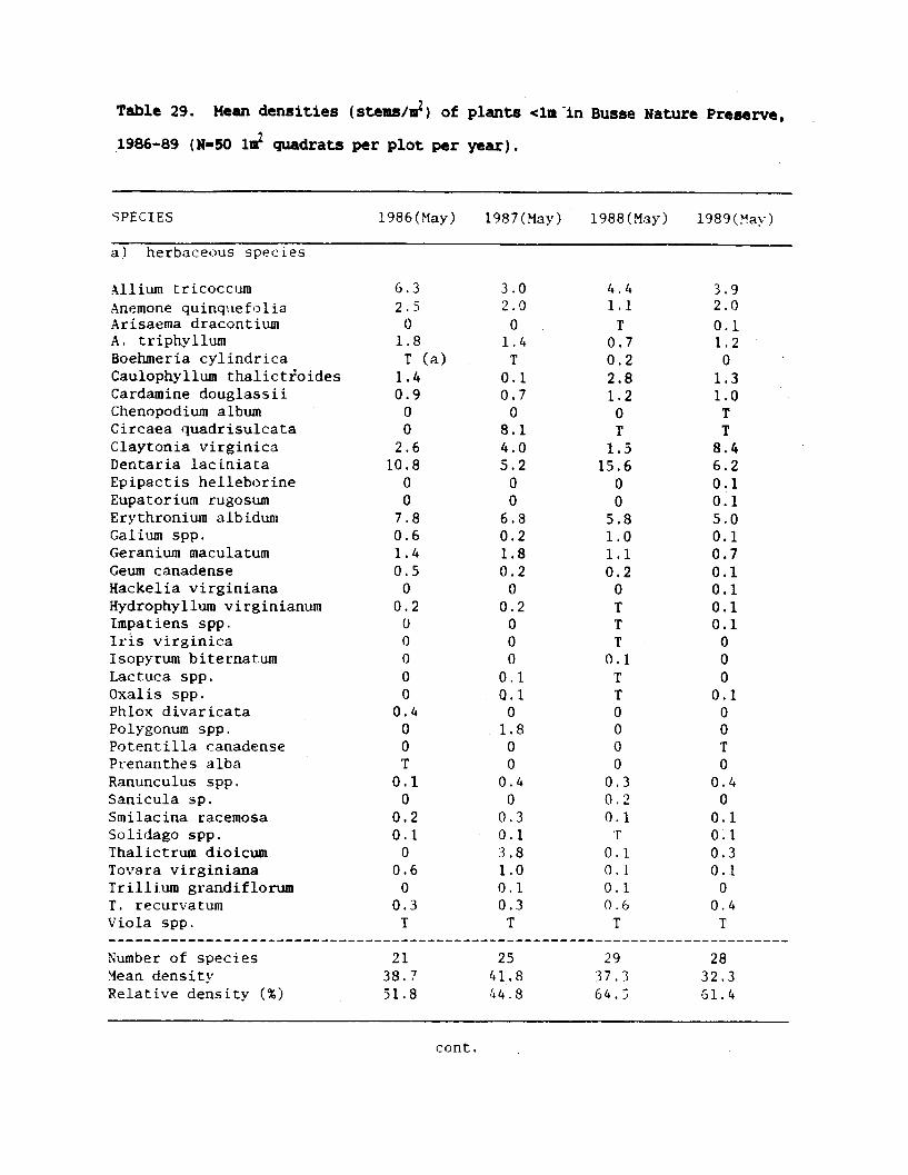
Table 29. Mean densities (stems/a 2) of plants <la in Busse Nature Preserve,
1986-89 (N=50 lu3 quadrats per plot per year).
SPECIES 1986(May) 1987(May) 1988(May) 1989(May)
a) herbaceous species
Allium tricoccum 6.3 3.0 4.4 3.9Anemone quinquefolia 2.5 2.0 1.1 2.0Arisaema dracontium 0 0 T 0.1A. triphyllum 1.8 1.4 0.7 1.2Boehmeria cylindrica T (a) T 0.2 0Caulophyllum thalictioides 1.4 0.1 2.8 1.3Cardamine douglassii 0.9 0.7 1.2 1.0Chenopodium album 0 0 0 TCircaea quadrisulcata 0 8.1 T TClaytonia virginica 2.6 4.0 1.5 8.4Dentaria laciniata 10.8 5.2 15.6 6.2Epipactis helleborine 0 0 0 0.1Eupatorium rugosum 0 0 0 0.1Erythronium albidum 7.8 6.8 5.8 5.0Galium spp. 0.6 0.2 1.0 0.1Geranium maculatum 1.4 1.8 1.1 0.7Geum canadense 0.5 0.2 0.2 0.1Hackelia virginiana 0 0 0 0.1Hydrophyllum virginianum 0.2 0.2 T 0.1Impatiens spp. 0 0 T 0.1Iris virginica 0 0 T 0Isopyrum biternatum 0 0 0.1 0Lactuca spp. 0 0.1 T 0Oxalis spp. 0 Q.1 T 0.1Phlox divaricata 0.4 0 0 0Polygonum spp. 0 1.8 0 0Potent illa canadense 0 0 0 TPrenanthes alba T 0 0 0Ranunculus spp. 0.1 0.4 0.3 0.4Sanicula sp. 0 0 0.2 0Smilacina racemosa 0.2 0.3 0.1 0.1Solidago spp. 0.1 0.1 T 0.1Thalictrum dioicum 0 3.8 0.1 0.3Tovara virginiana 0.6 1.0 0.1 0.1Trillium grandiflorum 0 0.1 0.1 0T. recurvatum 0.3 0.3 0.6 0.4Viola spp. T T T T
Number of species 21 25 29 28Mean density 38.7 41.8 37.3 32.3Relative density (%) 51.8 44.8 64.5 61.4
cont.
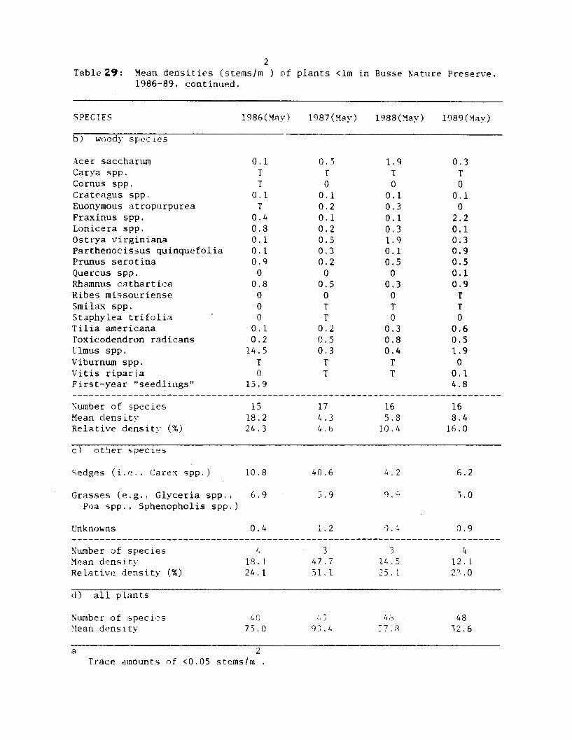
Table 29: Mean densities (stems/m ) of plants <lm in Busse Nature Preserve.1986-89, continued.
SPECIES 1986(May) 1987(May) 1988(May) 1989(May)
b) woody species
Acer saccharum 0.1 0.5 1.9 0.3Carya spp. T T T TCornus spp. T 0 0 0Crateagus spp. 0.1 0.1 0.1 0.1Euonymous atropurpurea T 0.2 0.3 0Fraxinus spp. 0.4 0.1 0.1 2.2Lonicera spp. 0.8 0.2 0.3 0.1Ostrya virginiana 0.1 0.5 1.9 0.3Parthenocissus quinquefolia 0.1 0.3 0.1 0.9Prunus serotina 0.9 0.2 0.5 0.5Quercus spp. 0 0 0 0.1Rhamnus cathartica 0.8 0.5 0.3 0.9Ribes missouriense 0 0 0 TSmilax spp. 0 T T TStaphylea trifolia " 0 T 0 0Tilia americana 0.1 0.2 0.3 0.6Toxicodendron radicans 0.2 0.5 0.8 0.5Llmus spp. 14.5 0.3 0.4 1.9Viburnum spp. T T T 0Vitis riparia 0 T T 0.1First-year "seedlings" 15.9 4.8
Number of species 15 17 16 16Mean density 18.2 4.3 5.8 8.4Relative density (%) 24.3 4.6 10.4 16.0
c) other species
Sedges (i.e., Carex spp.) 10.8 40.6 4.2 6.2
Grasses (e.g., Glyceria spp., 6.9 5.9 9.9 5.0Poa spp., Sphenopholis spp.)
Unknowns 0.4 1.2 3.4 0.9
Number of species 4 3 3 4Mean density 18.1 47.7 14.5 12.1Relative density (%) 24.1 51.1 25.1 23.0
d) all plants
Number of species 40 43 Au 48Mean density 75.0 93.4 37., 32.6
a 2Trace amounts of <0.05 stems/m .

Table 30. Mean percent cover of plants < la in Busse Nature Preserve during May
1986-1989; number of species shown in parentheses.
Plant Type 1986 1987 1988 1989
Herbaceous 1.9 (20) 1.8 (28) 2.9 (27) 2.9 (28)
Woody. 0.3 (14) 0.5 (13) 0.4 (13) 0.5 (13)a
First-year 0.2 NR (b) NR 0.2"seedlings"
c
Exotic Woody T (d) T T Te
Others 2.5 (5) 1.8 (6) 3.3 (6) 3.2 (7)
Total 4.7 (40) 4.1 (48) 6.7 (48) 6.6 (49)
a
b
C
d
e
Also included in the "Woody" category.
Not Recorded.
Includes Rhamnus cathartica and Berberis thunbergii.
Trace amounts of <0.05%.
includes grasses, sedges, mosses, unidentifiable species, and other obviouslyunpalatable species (i.e., Allium canadense, Allium tricoccum, Sanicula,anadensis, and Eupatorium rugosum).

Table 31. Mean percent cover of plants <lm in Busse Nature Preserve, 1986-89
(N=25 20a line intercepts per year).
SPECIES 1986(May) 1987(May) 1988(May) 1989(May)
a) herbaceous species
Allium canadense T (a) T T T
A. tricoccum 2.0 T 1.9 2.4
Anemone quinquefolia 0.1 0.1 0.1 0.1
Arisaema dracontium 0 0 0 T
A. triphyllum T 0.1 T 0.1
Boehmeria cylindrica 0 0.1 T 0
Caulophyllum thalictroides 0.4 0.7 0.6 0.5
Cardamine douglassii T T T T
Chenopodium album 0 0 0 T
Circaea quadrisulcata 0 T T T
Cirsium sp. 0 T 0 0
Claytonia virginica T T 0.1 0.1
Dentaria laciniata 0.8 0.2 1.4 1.1
Epipactis helleborine 0 0 T T
Eupatorium rugosum 0 0 0 T
Erythronium albidum 0.2 0.1 0.2 0.3
Galium spp. T T T 0.1
Geranium maculatum 0.1 0.1 0.2 0.1
Geum canadense T T T 0.1
Hydrophyllum virginianum 0 T 0 T
Iris virginica T 0.1 T 0.1
Isopyrum biternatum 0 0 T T
Lactuca spp. 0 T 0 0
Oxalis spp. 0 T 0 0
Phlox divaricata 0 0 0 T
Plantago spp. T T 0 0
Polygonum spp. 0 T T 0
Potentilla canadense 0 T T 0
Podophyllum peltatum T 0 0 0
Prenanthes alba 0 T T T
Ranunculus spp. T T T T
Sanicula sp. 0 0 T 0
Smilacina racemosa T T T T
Solidago spp. T T T T
Taraxacum officinale 0 0 0 T
Thalictrum dioicum 0.1 T T T
Tovara virginiana T 0.1 T 0.1
Trillium grandiflorum 0 0 T 0
T. recurvatum T T 0.1 0.1
Viola spp. T T T r
Number of species 22 30 29 30
lean % cover 3.9 1.39 4.9 5.4
Relative cover (%) 81.3 46.3 73.1 81.8
cont.

Table 31. (cont.)
SPECIES 1986(May) 1987(May) 1988(May) 1989(May)
b) woody species
Acer saccharum T T 0.1 T
Carya spp. 0 0 T 0
Cornus spp. T 0 T TCrateagus spp. r T T TEuonymous atropurpurea T T T TFraxinus spp. T T T 0.1Lonicera spp. 0.1 0.1 T TOstrya virginiana T 0.1 T TParthenocissus quinquefolia T T T 0.1Prunus serotina T T 0.1 T
Quercus spp. 0 0 0 T
Rhamnus cathartica T T T 0.1
Rubus spp. 0 0 0.1 0
Smilax spp. 0 T 0 T
Tilia americana T T T 0.1Toxicodendron radicans T T T 0.1
Ulmus spp. 0.2 0.1 T TViburnum spp. T 0 0 0
Vitis riparia T T 0 0
First-year "seedlings" 0.2 0.2
Number of species 15 14 15 15
Mean % cover 0.4 0.5 0.5 0.5
Relative cover (%) 8.3 12.2 7.5 7.6
c) other species
Sedges (i.e., Carex spp.) 0.3 0.6 0.7 0.5
Grasses (e.g., Glyceria spp., 0.1 0.3 0.3 0.1
Poa spp., Sphenopholis spp.)
Unknowns 0.1 0.1 T 0.1
Mosses 0.8 0.3------------------------------------------------------------
Number of species 3 4 4 4
Mean % cover 0.5 1.7 1. 0.7
Relative cover (%) 10.4 41.5 19.4 10.6
d) all plants
Number of species 40 48 48 49
Mean % cover 4.7 4.1 6.7 6.6
a 2
Trace amounts of <0.05 stems/m .

Table 32. Mean densities (stems/ 2 ) of plants < la in Busse Woods South during
April-May 1986-1987; number of species shown in parentheses.
Plant Type 1986(April) 1987(May)n=30 n=30
Herbaceous 94.5 (18) 80.1 (18)
Woody 3.5 (14) 3.2 (16)a
First-year 0.2 NR (b)c
Exotic Woody 0.4 (1) 0.2 (1)d
Others 20.5 (8) 12.8 (5)
Total 118.9 (41) 98.1 (40)
a
b
c
d
Included in the "Woody" category also.
Not Recorded during sampling.
includes Rhamnus cathartica.
includes grasses, sedges, unidentifiable species, and otherobviously unpalatable species (i.e., Allium canadense,and Allium tricoccum).

Table 33. Mean percent cover of plants < la in Busse Woods South during April-May 1986-1987. The number of species found is shown in parentheses. The samplesize was 15-20m permanent line intercepts per year.
Plant Type 1986(April) 1987(May)
Herbaceous 5.2 (16) 9.1 (24)
Woody 0.8 (15) 4.5 (16)a
Exotic Woody 0.2 (1) 0.6 (1)b
Others 0.7 (5) 1.9 (5)
Total 6.9 (37) 16.0 (46)
aincludes Rhamnus cathartica.
bincludes grasses, sedges, mosses, unidentifiable species, and
other obviously unpalatable species (i.e., Alliumcanadense, and Allium tricoccum).
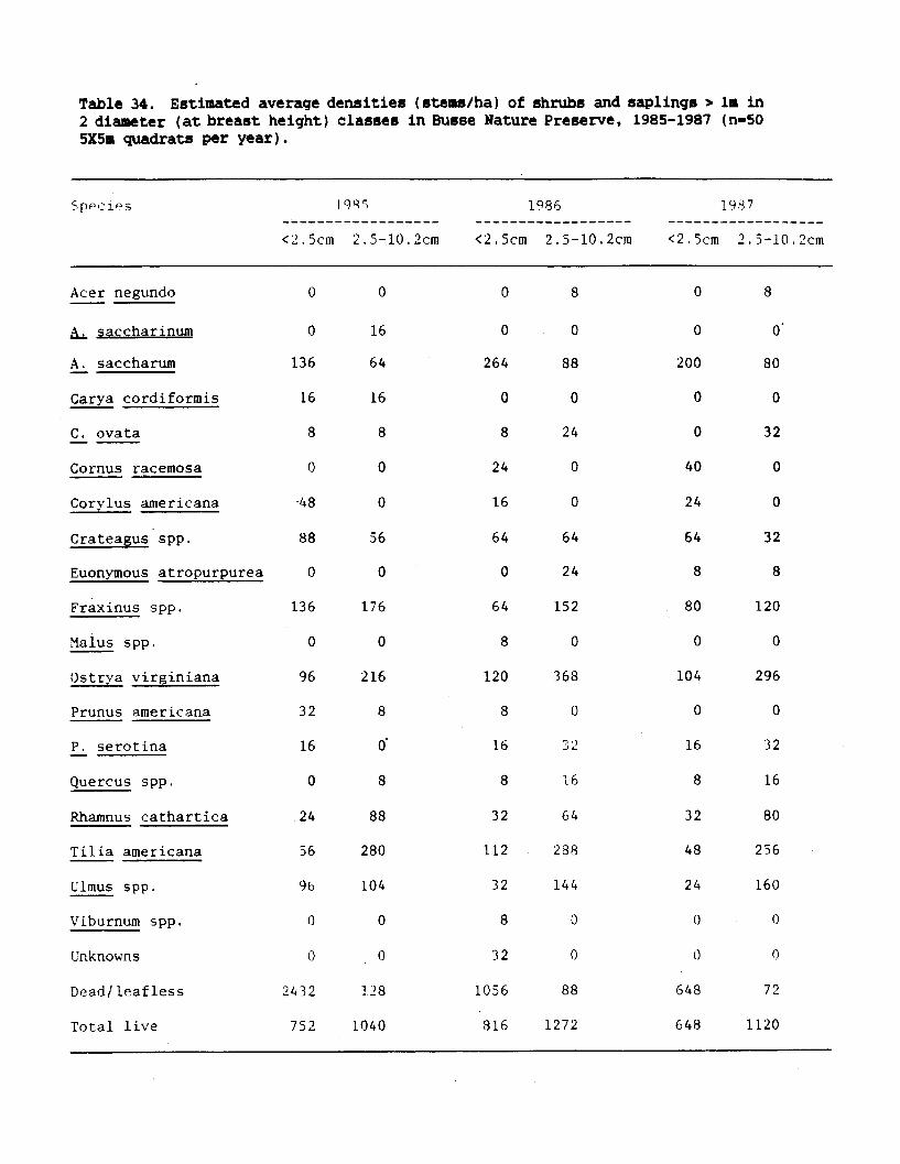
Table 34. Estimated average densities (stems/ha) of shrubs and saplings > la in2 diameter (at breast height) classes in Busse Nature Preserve, 1985-1987 (n-505X5a quadrats per year).
Species 1985 186 1987
<2.5cm 2.5-10.2cm <2.5cm 2.5-10.2cm <2.5cm 2.5-10.2cm
Acer negundo 0 8
A. saccharinumr
A. saccharum
Carya cordiformis
C. ovata
Cornus racemosa
Corylus americana
Crateagus spp.
Euonymous atropurpurea
Fraxinus spp.
Malus spp.
Ostrya virginiana
Prunus americana
P. serotina
Quercus spp.
Rhamnus cathartica
Tilia americana
Ulmus spp.
Viburnum spp.
Unknowns
0
136
16
64
16 16
8
0
-48
88
0
136
0
96 216
32
16
0
56
0
176
0
264
0
88
0
8 24
24
16
64
0
0
200
0
0
40
24
64
8
80
64
24
64 152
0
120 368 104
08
0O
24 88
56 280
96 104
1616 32
8 16
32
112
64
288
32 144
32
32
48
0
80
0
32
0
0
32
8
120
0
296
0
32
16
80
256
24 160
0
Dead/leafless 2432 128 1056 88 648 72
752 1040 816 1272 648 1120Total live

Table 35. Estimated average densities (stems/ha) of shrubs and saplings >1l in2 diameter (at breast height) classes in Busse Woods South, 1985-1986 (n-25 5X5mquadrats in 1985 and 30 quadrats in 1986).
Species 1985 1986
<2.5cm 2.5-10.2cm <2.5cm 2.5-10.2cm
Acer saccharum 1472 368 1307 307
Carya cordiformis 16 0 93 0
C. ovata 80 0 53 13
Cornus spp. 48 0 0 0
Corylus americana 16 0 13 0
Crateagus spp. 208 48 93 0
Fraxinus spp. 128 48 107 13
Malus spp. 0 0 13 0
Ostrya virginiana 160 208 120 280
Prunus americana 224 0 0 0
P. serotina 16 16 0 0
Quercus spp. 48 0 0 0
Rhamnus cathartica 128 64 347 80
Tilia americana 448 352 320 200
Ulmus spp. 176 144 67 187
Viburnum spp. 0 0 27 0
Xanthoxylum americanum 192 16 267 13
Dead/leafless 784 160 627 67
Total live 3360 1264 2827 1107
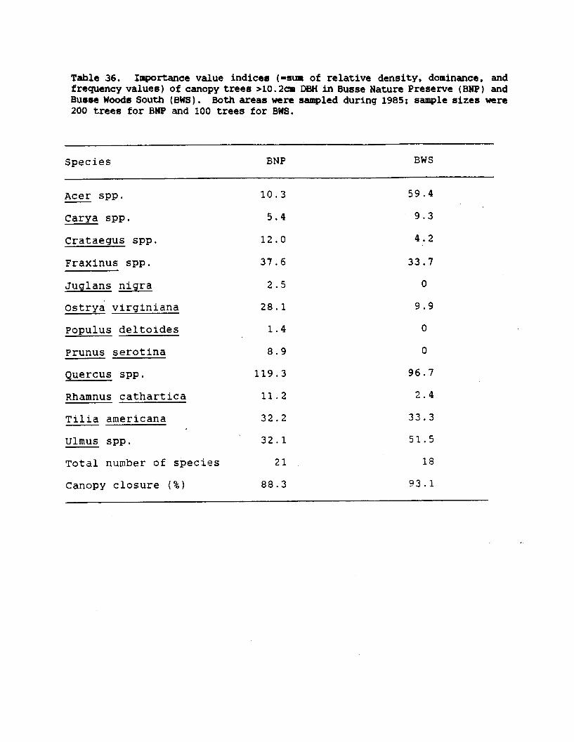
Table 36. Importance value indices (=sun of relative density, dominance, andfrequency values) of canopy trees >10.2cm DBH in Busse Nature Preserve (BNP) andBusse Woods South (BWS). Both areas were sampled during 1985; sample sizes were200 trees for BNP and 100 trees for BWS.
Species BNP BWS
Acer spp. 10.3 59.4
Carya spp. 5.4 9.3
Crataegus spp. 12.0 4.2
Fraxinus spp. 37.6 33.7
Juglans nigra 2.5 0
Ostrya virginiana 28.1 9.9
Populus deltoides 1.4 0
Prunus serotina 8.9 0
Quercus spp. 119.3 96.7
Rhamnus cathartica 11.2 2.4
Tilia americana 32.2 33.3
Ulmus spp. 32.1 51.5
Total number of species 21 18
anrnvy clsucir (% ) 88.3 93.1*f CA L.. A ~ % L- y % .La -. )%A J .-. \ % -0 %-f w a If
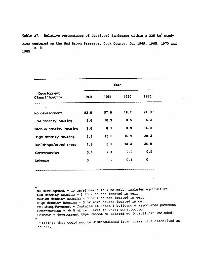
Table 37. Relative percentages of developed landscape within a 225 km2 study
area centered on the Ned Brown Preserve, Cook County, for 1949, 1965, 1970 anda, b
1985.
Year
DevelopmentClassification 1949 1964 1970 1985
No development 82.6 57.9 49.7 24.8
Low density housing 9.6 10.3 8.6 5.3
Medium density housing 3.6 6.1 8.0 14.9
High density housing 2.1 15.0 16.9 29.2
Buildings/paved areas 1.8 8.2 14.4 24.9
Construction 0.4 2.4 2.2 0.9
Unknown 0 0.2 0.1 0
aNo development - no development in 1 ha cell, includes agriculture
Low density housing - 1 to 2 houses located in cell
Medium density housing = 3 or 4 houses located in cell
High density housing = 5 or more houses located in cell
Building/Pavement = Contains at least 1 building & associated pavement
Construction = >0.5 of cell area is under construction
Unknown = development type cannot be determined (gravel pit included)
bBuildings that could not be distinguished from houses were classified
as
houses.

Table 38. Relative percentages of road types within a 225 km2 study area
centered on the Ned Brown Preserve, Cook County, for 1949, 1965, 1970 anda, b
1985.
Year
RoadClassification 1949 1964 1970 1985
No roads 77.7 59.0 53.6 44.2
Secondary 10.4 30.8 35.0 43.8
Main 10.8 6.0 6.9 5.9
Major 0.0 1.2 1.4 1.6
Secondary/Main 1.1 2.6 2.4 3.6
Main/MaJor 0 0.3 0.3 0.6
Secondary/Major 0 0.2 0.3 0.4
aDefinitions:
No roads = no roads in cellSecondary roads = all roads that are not main or major roads includes RRMain roads = 2 or 4 lane roads >5 km in lengthMajor highways - roads with > 5 lanesSecondary/Main = both types are located in cellMain/Major = both types are located in cellSecondary/Major = both types are located in cell
bDriveways, gravel, and dirt roads were not classifiedcRoads under construction categorized by type at completion

Table 39. Relative percentages of vegetation types within a 225 km2 study
area centered on the Ned Brown Preserve, Cook County, for 1949, 1965, 1970 anda, b
1985.
Year
VegetationClassification 1949 1964 1970 1985
No vegetation 0.1 2.2 5.4 19.3
Agricultural field 79.9 41.5 24.9 5.2
Grass 5.1 24.5 25.1 29.0
Mixed vegetation 13.8 30.4 43.0 39.5
Closed canopy forest 0.9 1.3 1.6 6.4
Unknown 0 0 0 0.1
Definitions.
No vegetation = no dominant vegetation in cellAgricultural field = at least 0.5 of cell is cropland or pastureGrass = meadow or grass not associated with agricultureMixed vegetation = mixture of grass, shrubs, marsh, and/or treesClosed canopy forest = entire cell includes closed canopy woodlotUnknown = type not distinguishable from aerial photograph

Table 40. Relative percentages of water resources within a 225 km2 study area
centered on the Ned Brown Preserve, Cook County, for 1949, 1965, 1970 anda, b
1985.
Year
WaterResource 1949 1964 1970 1985
Classification
No water 86.1 92.2 88.9 90.2
Stream 7.5 4.6 4.9 3.5
Shoreline 1.2 1.3 2.6 4.7
Open water 1.1 0 0.1 0.5
Marsh shoreline 4.2 1.9 3.6 1.2
Open marsh 0 0 0 0
aDefinitions:
No water = no water identified in cell
Stream = segment of stream <100 m in width in cell
Shoreline - interface between land and lake, pond, or river >100 m width
Open water entire cell is open water
Marsh shoreline = interface between land and marsh in cell
Open marsh = entire cell is marsh

Table 41. Mean cost of deer-vehicle accidents in Cook County, Illinois, duringa,b,c
1984 to 1988.
CostCategory Mean SE Range of Valuesby Year
1984
N = 140 usable responses
Vehicle repairTowingSubstitute vehicleMedicalLost wagesOtherTotal cost (d)
1985
N = 79 usable responses
$ 1,149.4410.4035.2513.5717.350.77
1,226.78
Vehicle repairTowingSubstitute vehicleMedicalLost wagesOtherTotal cost (d)
$ 1,328.7110.6540.8426.6133.386.13
1,446.32
133.612.53
11.7613.4919.834.93
156.65
0.000.000.000.000.000.0055.00
- 8,010.25- 125.00- 565.00- 752.00- 1,500.00- 384.00-10,387.25
1986
N = 94 usable responses
Vehicle repairTowingSubstitute vehicleMedicalLost wagesOtherTotal cost (d)
$ 1,470.6613.5583.0018.3728.149.04
1,622.77
183.332.71
22.268.0311.784.66
194.84
0.000.000.000.000.000.000.00
-13,200.00- 115.00- 1,700.00- 500.00- 800.00- 300.00-14,050.00
(cont.)
78.342.258.7210.8211.370.47
92.10
0.000.000.000.000.000.000.00
6,240.00150.00600.00
1,500.001,500.00
45.007,340.00

Table 41. (cont.)
CostCategory Mean SE Range of Valuesby Year
1987
N = 118 usable responses
Vehicle repair $ 1,247.03 98.36 0.00 - 8,000.00Towing 9.26 2.41 0.00 - 130.00Substitute vehicle 57.46 11.25 0.00 - 509.00Medical 1.56 1.15 0.00 - 131.00Lost wages 4.15 2.20 0.00 - 150.00Other 31.66 14.28 0.00 - 1,500.00Total cost (d) 1,351.13 109.43 10.00 - 8,621.00
1988
N = 110 usable responses
Vehicle repair $ 1,478.38 133.20 0.00 - 8,900.00Towing 9.65 2.37 0.00 - 125.00Substitute vehicle 73.18 13.53 0.00 - 825.00Medical 9.76 5.36 0.00 - 507.60Lost wages 11.40 6.20 0.00 - 550.00Other 17.82 12.10 0.00 - 1,300.00Total cost (d) 1,600.18 144.21 10.00 -10,157.00
aQuestionnaires were sent to individuals involved in deer-vehicle accidentsthat were investigated by the Cook County Sheriff's Police.
Responses in 1984 include X deer-vehicle accidents investigated bymunicipality police departments; total cost of these accidents was notsignificantly different from costs derived from Cook County Sheriff's Policeresponses.
Cost in U.S. dollars
Total Cost was determined by averaging the Total Cost of individualresponses. Therefore, the Range of Values for Total Cost can have a minimumvalue > $ 0.00 even though the minimum value for each cost category (e.g.,repair, towing etc.) was = $ 0.00.
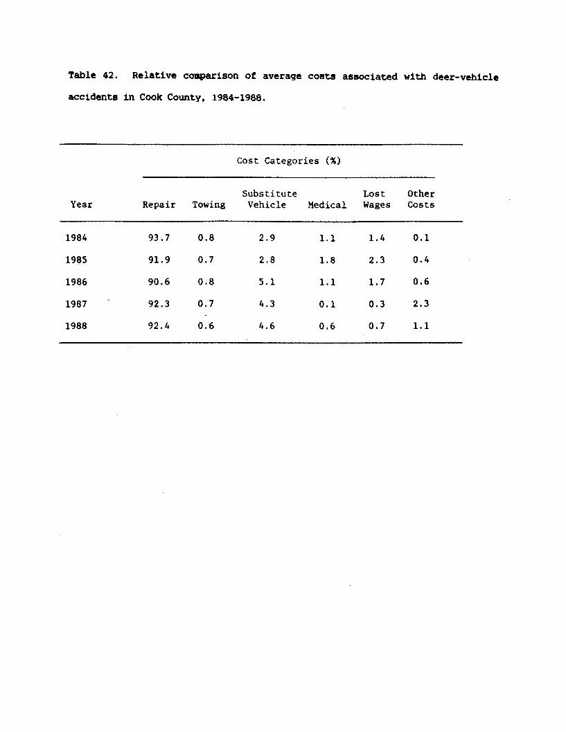
Table 42. Relative comparison of average costs associated with deer-vehicle
accidents in Cook County, 1984-1988.
Cost Categories (%)
Substitute Lost OtherYear Repair Towing Vehicle Medical Wages Costs
1984 93.7 0.8 2.9 1.1 1.4 0.1
1985 91.9 0.7 2.8 1.8 2.3 0.4
1986 90.6 0.8 5.1 1.1 1.7 0.6
1987 92.3 0.7 4.3 0.1 0.3 2.3
1988 92.4 0.6 4.6 0.6 0.7 1.1

Table 43. Number of deer-vehicle accidents reported on state-numbered highways
in northeastern Illinois from 1978 through 1990 (Ill. Dep. Trans.)
Year
County 78 79 80 81 82 83 .84 85 86 87 88 89 90
Cook 137 112 139 167 260 248 354 379 469 436 494 499 610
DuPage 20 19 19 20 23 31 50 58 76 72 85 74 109
Kane 24 34 36 36 55 68 80 81 124 125 150 190 216
Lake 66 50 53 73 105 126 157 200 250 274 298 359 346
Total 247 215 247 296 443 473 641 718 919 907 1027 1122 1281

Table 44. Sex and age composition of all deer removed by INHS from the Ned Brown
Preserve, Cook County, from 1983 to 1988. Methods used included live-capture by
rocket net, drive net, and sharpshooting.
Female MaleAutumn-Winter
Fawns Yearlings Adults Fawns Yearlings Adults
1983-1984 2 1 7 0 0 0
1984-1985 6 3 9 6 0 1
1985-1986 23 3 42 36 8 13
1986-1987 35 14 40 33 13 7
1987-1988 10 7 15 11 8 10
1988-1989 2 0 2 2 0 0
Totals 78 28 115 88 29 31

Table 45. The minimum number of deer counted during helicopter surveys during
winter and the number of deer removed by INHS annually at the Ned Brown
Preserve from 1983-84 to 1988-89.
1983-84 1984-85 1985-86 1986-87 1987-88
Aerial countNorth NB 258 207 154 85 47South NB 35 46 36 33 56
Minimum densityNorth NB 37 30 22 12 7South NB 4 6 5 4 7Total NB 20 17 13 8 7
No. deer removed 10 25 125 142 61

Table 46. Annual deer-vehicle accident rates for selected highways from 4
locations in Cook County during 1982-1988.
Accidents/kmLength of highways
Area evaluated (km) 1982 1983 1984 1985 1986 1987 1988
Ned Brown 24.1 1.45 1.0 1.41 0.91 0.83 0.46 0.42
Northwest 41.8 0.50 0.62 0.84 0.71 0.93 0.88 0.88
Des Plaines 25.7 0.89 0.58 0.89 1.05 1.05 0.74 0.86
Palos 37.0 0.92 0.60 1.02 0.94 1.13 0.73 0.89

Table 47. Correlation matrix comparing the frequencies of deer-vehicle accidents
at locations in Cook County. Accident frequency data were from Illinois
Department of Transportation summaries (1982-1988) for selected road sections
within each area.
Area
AreaNed Brown Northwest Cook Des Plaines Palos Cook
Ned Brown 1.0
Northwest Cook -0.63 1.0
Des Plaines 0.13 0.25 1.0
Palos 0.24 - 0.37 0.91 1.0
aCook -0.75 0.90 0.42 0.43 1.0
(-0.79) (0.89) (0.39). (0.37)
aCorrelation coefficients in parentheses were determined by comparing subcounty(e.g., Palos) accident frequencies with those from Cook County that were reducedby the number of accidents in the subcounty of comparison.
Example: (Palos accidents) vs (Cook County total accidents - Palos accidents)
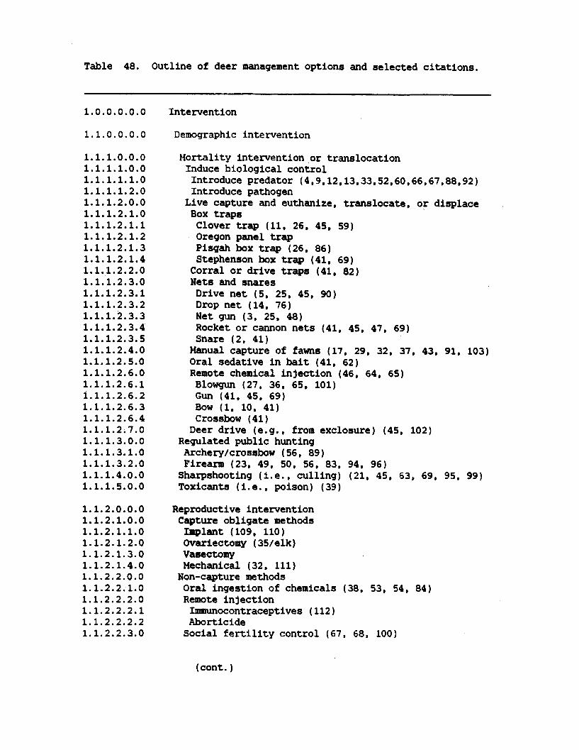
Table 48. Outline of deer management options and selected citations.
1.0.0.0.0.0
1.1.0.0.0.0
1.1.1.0.0.01.1.1.1.0.01.1.1.1.1.01.1.1.1.2.01.1.1.2.0.01.1.1.2.1.01.1.1.2.1.11.1.1.2.1.21.1.1.2.1.31.1.1.2.1.41.1.1.2.2.01.1.1.2.3.01.1.1.2.3.11.1.1.2.3.21.1.1.2.3.31.1.1.2.3.41.1.1.2.3.51.1.1.2.4.01.1.1.2.5.01.1.1.2.6.01.1.1.2.6.11.1.1.2.6.21.1.1.2.6.31.1.1.2.6.41.1.1.2.7.01.1.1.3.0.01.1.1.3.1.01.1.1.3.2.01.1.1.4.0.01.1.1.5.0.0
1.1.2.0.0.01.1.2.1.0.01.1.2.1.1.01.1.2.1.2.01.1.2.1.3.01.1.2.1.4.01.1.2.2.0.01.1.2.2. 1.01.1.2.2.2.01.1.2.2.2.11.1.2.2.2.21.1.2.2.3.0
Intervention
Demographic intervention
Mortality intervention or translocationInduce biological controlIntroduce predator (4,9,12.13,33.52,60.66,67,88,92)Introduce pathogen
Live capture and euthanize, translocate, or displaceBox trapsClover trap (11, 26, 45. 59)Oregon panel trapPisgah box trap (26, 86)Stephenson box trap (41, 69)
Corral or drive traps (41, 82)Nets and snaresDrive net (5, 25, 45, 90)Drop net (14, 76)Net gun (3, 25. 48)Rocket or cannon nets (41, 45, 47, 69)Snare (2, 41)Manual capture of fawns (17, 29. 32. 37. 43. 91. 103)Oral sedative in bait (41, 62)Remote chemical injection (46, 64. 65)Blowgun (27, 36, 65. 101)Gun (41, 45. 69)Bow (1, 10, 41)Crossbow (41)
Deer drive (e.g., from exclosure) (45, 102)Regulated public huntingArchery/crossbow (56, 89)Firearm (23, 49, 50, 56, 83, 94. 96)Sharpshooting (i.e., culling) (21, 45, 63, 69, 95, 99)Toxicants (i.e., poison) (39)
Reproductive interventionCapture obligate methodsImplant (109. 110)Ovariectomy (35/elk)VasectomyMechanical (32, 111)Non-capture methodsOral ingestion of chemicals (38, 53, 54. 84)Remote injectionImmunocontraceptives (112)AborticideSocial fertility control (67, 68, 100)
(cont.)

Table 48. (cont.)
1.2.0.0.0.0
1.2.1.0.0.01.2.1.1.0.01.2.1.1.1.01.2.1.1.2.01.2.1.1.2.01.2.1.2.0.01.2.1.3.0.0
1.2.2.0.0.01.2.2.1.0.01.2.2.1.1.01.2.2.1.2.01.2.2.1.3.01.2.2.2.0.01.2.2.2.1.01.2.2.2.1.11.2.2.2.1.21.2.2.2.1.31.2.2.2.1.41.2.2.2.1.51.2.2.2.1.61.2.2.2.1.71.2.2.2.1.81.2.2.2.2.01.2.2.2.2.11.2.2.2.2.21.2.2.2.2.31.2.2.2.2.41.2.2.2.2.51.2.2.2.2.61.2.2.2.2.71.2.2.2.3.01.2.2.2.3.11.2.2.2.3.21.2.2.2.3.31.2.2.2.3.41.2.2.2.4.01.2.2.2.4.11.2.2.2.4.2
2.0.0.0.0.02.1.0.0.0.02.1.1.0.0.02.1.2.0.0.02.1.3.0.0.02.2.0.0.0.0
NoninterventionCognizant inactionAcceptance of problemAvoidance of decisionCompensation (e.g.. monetary) (93)
Incognizance or no recognized problem
(cont.)
Habitat and/or behavior modification
Modify habitat characteristicsProvide supplemental, diversionary, or attractant foodsProvide feed (6,7,22,28,42,68,87,104,105,106,107)Fertilize (20, 61, 97)Seed/plantRoad modification (77, 79)Decrease carrying capacity via silviculture (16, 75)
Modify deer use of habitat resourcesExclusionElectric fence (8, 18, 44, 51, 58, 71, 73, 98)Non-electric fence (18, 30, 31, 51, 71, 78)Mechanical barriers to protect individual plants (24,40,45)Repellents and warning devicesArea (i.e., smell)Feather meal (70)Human hair (15, 89)Meat meal (70)Predator odors (57)Putrescent egg solidsSoap (89)Tankage (89)OtherContact (i.e., taste) (19)Ammonium soaps of higher fatty acidesBenzyl diethyl methyl ammonium saccharide, thymolBone tar oilCapsaicin (15, 70, 89)Putrescent egg solidsThiramOtherAuditory (i.e., hearing)Dog (89)Exploder (18, 89)Gun discharge (89)Vehicle whistleVisual (i.e., sight)Road mirrors/reflectors (34,72,74,80,81,85,108)Scarecrow (89)

Table 48. (cont.)
1) Anderson 1961, 2) Ashcraft and Reese 1957, 3) Barrett et al. 1982, 4)Beasom 1974, 5) Beasom et al. 1980, 6) Brown and Mandery 1962, 7) Carhart1943, 8) Caslick and Decker 1979, 9) Causey and Cude 1980, 10) Causey et al.1978, 11) Clover 1956, 12) Connolly 1978, 13) Connolly 1981, 14) Connor et al.19870 15) Conover 1984, 16) Conover 1988, 17) Cook et al. 1971, 18) Craven1983, 19) Crawford and Church 1971, 20) Crouch and Radwan 1981, 21) Dalbergand Guettinger 1956, 22) Dasmann et al. 1967, 23) Dechert 1967, 24) DeVoe andSchaap 1983, 25) DeYoung 1988, 26) Diehl 1988, 27) Dinnes 1982, 28) Doman andRasmussen 1944, 29) Downing and McGinnes 1969, 30) Falk et al. 1978, 31)Feldhammer et al. 1986, 32) Garrott and Bartmann 1984, 33) Gavitt et al. 1974,34) Graves and Bellis 1978, 35) Greer 1968 (elk), 36) Haigh and Hopf 1976, 37)Hamlin et al. 1984, 38) Harder and Peterle 1974, 39) Harris 1984s55. 40)Hawthorne 1980, 41) Hawkins et al. 1967, 42) Hubert et al. 1980, 43) Huegel etal. 1985, 44) Hygnstrom and Craven 1988, 45) Ishmael and Rongstad 1984, 46)Jessup et al. 1983, 47) Jones and Witham 1990, 48) Krausnman et al 1985, 49)Krefting et al. 1955, 50) Krefting and Erickson 1956, 51) Longhurst et al.1962, 52) Lowry and McArthur 1978, 53) Matschke 1977a, 54) Hatschke 1977b, 55)Matschke et al. 1984, 56) Martin and Krefting 1953, 57) Melchiors and Leslie1985, 58) McAtee 1939, 59) McCullough 1975, 60) Mech 1984, 61) Mitchell andHosley 1936, 62) Montgomery and Hawkins 1967, 63) Moore et al. 1977, 64)Nielsen 1982, 65) Nielsen 1989, 66) Nesbitt 1975, 67) Ozoga et al. 1982, 68)Ozoga and Verme 1982, 69) Palmer et al. 1980, 70) Harris et al. 1983, 71)Palmer et al. 1985, 72) Pojar et al. 1975, 73) Porter 1983, 74) Queal 1968,75) Radwan 1972, 76) Ramsey 1968, 77) Reed 1981, 78) Reed et al. 1974, 79)Reed et al. 1975, 80) Reed and Woodard 1981, 81) Reed et al. 1982, 82) Rempeland Bertram 1975, 83) Roseberry et al. 1969, 84) Roughton 1979, 85) Schaferand Penland 1985, 86) Schilling 1938, 87) Schoonveld et al. 1974, 88) Scottand Causey 1973, 89) Scott and Townsend 1985, 89) Severinghaus 1963, 90) Silvyet al. 1975, 91) Steigers and Flinders 1980, 92) Stout 1982, 93) Strickland1976, 94) Swank 1962, 95) Taylor and Katahira 1988 (goats), 96) Teer et al.1965, 97) Thomas et al. 1964, 98) Tierson 1969, 99) Van Etten et al. 1965,100) Verme et al. 1987, 101) Warren et al. 1979, 102) Wemmer and Stuwe 1985,103) White et al. 1972, 104) Woebeser and Runge 1975, 105) Wood and Wolfe1988, 106) Woolf and Harder 1979, 107) Woolfe 1977, and 108) Zacks 1986, 109)Botti 1985, 110) Bell and Peterle 1975, 111) Matschke 1976, 112) Turner et al.1992.

LIST OF FIGURES1. The INHS Urban Deer Program 4-county study area.
2. Location of 5 substudy areas used for nutrition research in the CMA.
3. Woodlots sampled within the Ned Brown Preserve.
4. Distribution of deer sightings in Kane County by fixed wing aircraft.
5. Mean stem densities of all herbaceous species.
6. Mean stem density of woodland knotweed.
7. Mean stem density of all woody species.
8. Mean percent cover of white adder's tongue.
9. Mean percent cover of woodland knotweed.
10. Mean percent cover of wakerobin.
11. Mean percent cover of all woody species.
12. Potential deer habitat in Cook County.
13. Potential deer habitat in DuPage County.
14. Potential deer habitat in Kane County.
15. Potential deer habitat in Lake County.
16. Distribution of deer-vehicle accidents in Lake County.
17. Distribution of deer-vehicle accidents in Kane County.
18. Distribution of deer-vehicle accidents in DuPage County.
19. Distribution of deer-vehicle accidents in Cook County.
20. Deer removal rates by sharpshooters at O'Hare Airport, 1988.
21. Regression for deer removed by sharpshooters at O'Hare Airport, 1988.
22. Sex and age composition of deer removed at O'Hare Airport, 1988.
23. Regression for deer live-captured at Ryerson Conservation Area, 1989.
24. Live trapping rates at Ryerson Conservation Area, 1989.
25. Regression for deer removed by sharpshooters at Ryerson, 1989.
26. Deer removal rates by sharpshooters at Ryerson, 1989.
27. Hypothetical recovery of plants in control vs. recovery in exclosure.

Fig. 1. Four-county study area of the INHS Urban Deer Research Prograa.

NON-COOK
Fig. 2. Deer condition was compared among 5 substudy areas (Des Plaines, NedBrown, Non-Cook, Northwest, and Palos) in the Chicago metro area.

rve, CCFPD.
Bussse Woods. No4aN.sture- PrQserv° ( slU-.py
Scale: 1 inch=4 mile
.OsurEntro.
3
NUWE
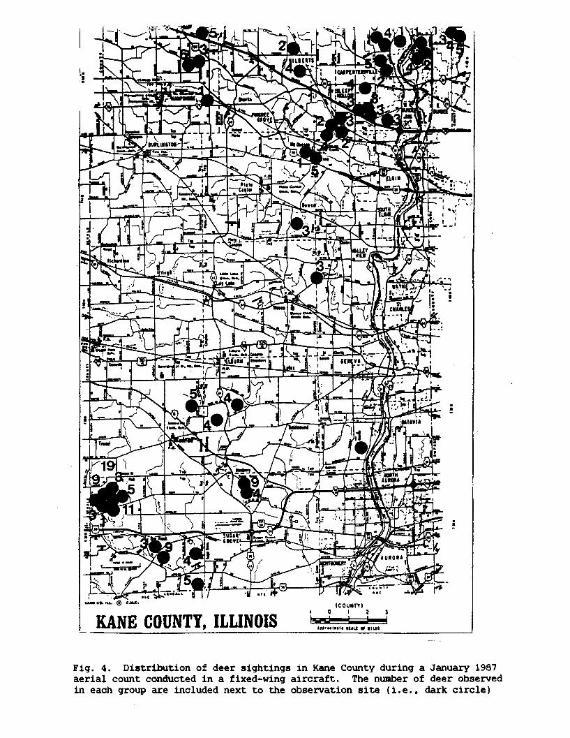
S 2 .A'., , 1-4). w)
Y Yet TifJURNA*Now_
FameftMR 14SNOVES 0
KAM CO.O . C CL. (COUNTY)
KANE COUNTY, ILLINOIS Il 4
Fig. 4. Distribution of deer sightings in Kane County during a January 1987aerial count conducted in a fixed-wing aircraft. The number of deer observedin each group are included next to the observation site (i.e., dark circle)
S.l low As"OvBURLINGTON a mfw* ewký % I .- w
[LOINPlot$csý 4tELSIN-
IdPoo- I - - % too
vow lot I
oak 0040
Luft %Abe Iammm, awbeIf LobMILE
Howlow* IMAOsm, tooSCLEURN wan HNEVA
00 fAT VITf"

I ~ ii*i ~ ICDI. 1.11.11tH. [II. '.1111 11 CCCI CR Ci H
DII~II llDlDllDUDllhi
.... .......... ... .................. ......... .. .. ..... .... ........ ........ ............ ............ . ............... . .......................... ............... ...... .. ...... ....; ..(" " ; l 1-; -
am,
it9; ,q.,,:"i
li
I-a
0
tor4w
IP
1.61.1
."..I
............ ...................... ..
C ;;;:; 1;^;;,"T o:o:
vul101..1

I .iIl .ll..ll
.T.tIITu1[
^^ ...... ....... ........ .......... ..... ........ .... ............... .....1-4' Wo- ef^ -
2> ::£: L."; a^
04U111
, 1.
C;....;
14 I
Uv oil
IGM
..Il..l,. .II.,..
.............................. i ..... q I --ilO*ll * * if • * I!1 o It * • I1 * •ll# lio * il ' * li* otl * Oil* *ltooli* * Ilillll °• I oil * °lll0il
| *l]**il*•i*•, an•N, •l•ll.ll• I--•I*•| A .no •il**il• •11..11• ,ll• oil. oil, oli•lh olaqll* o ilool| *-nu-oll•*H*0 H Nlloatio*il *, I1. oti** i I o* II, *Ha oll * *H•olI*•I*olI* * It* • ol4*dio * n, ,No d5 all,, It•dl,,14, I | *•4io4b di**H* *U, Aalio*il* dINlldloall*tlt0tll N lo*ll*qli**llo It
• llr.il."u..i. .iT..ifnoiI'll*-'I10*HH"IT"H-1ll"tf,.u,'r •iI"II"H"H"H"'ll"ll"Ulll"tll
.i ,. L . ,..i t.,i.. ,,i..it1.1 I..R..R..I.n.l I..l...II II.. I1. I.1 l..1
10
0
*4
4.)
IO
0'"4
I.. .. . .IIS. . .............. .......... ............... 1- ...................... . . . . . . . . . . .
r"-CD"en"9**I

S . .... . .ifl i0m
.. ." i 41 1" ''i i• i 'JL'ii I".l 1i/ it:l[ t . Jl fIJ J I i 4 L L L L t I J L I., : :, i , : : • : , ' , ,! , ,,01 lei If if '11 of ,lot 0 if V1 ill All" ,
'I'.".... ti.." .l'" a ,. , L ...... ,iti.s... ..,. , .. t t I,.' '4 , ..i l.. l: . I ;IIoi.. .... i.. , ;. ,i t i. . .t,. l.. t .. . .t
Art"oil
---r-- Oor er irit .010 ee04pole, to' I .08A to,'11 10114 sit 01 1#1 foe 4X of 'sOoo ;"# ooll Pee Vto Voo ",,I0
,1 '
........... I....
I~~~~ XI -+ -- + -+
(J"l
,'-I
OV
r"%
r4
*?A
.1-
^ 4'03 »
[.. ..i .. ....
!?0 10,", ...... I ', ... .. ,," jO ., IT ,M 0 ,, ..... 'C -i".,,j , ,,,,,.| ,,.,^ ,, n.,| .......I .1- 1I
! , , , ..Ii.1 !• , i' ,, , it * . ' I

**CO!T"'sw-1
94
0
1.4
"4
8.
*O
00
*e
v4
fIj:
..4 ' ̂ ir,,.I : ": ,* ;: *.. ... .... ;;i'"^ ,^ fl ii fill
..... . ...... ... ......... .
M11-.
'Illlll*
(J .......1,
:X:
,:::L.,.»

Ii",
.............. . ..... ...... ..................
,i # tMs,* i !: 1: " ..- .;;" 1.": W
@"" *
4,,,.".
r**Ti S
e1"0 0
Li 5.4
0
L).n4.)
8.
^',4'
*O»-r4
111 ,.... A .. ............ .................. ........... .... .

Lfl 4
0'-4
.......................................... ........ ...................... ....................................... ............................................. .
I n
Ili .....41,,.,,.:i.',
l. .....-. ............................]*"< ;TS'i
CD
T 04,
I
..... ... .... u

"'<" e .4 11
LI41 jll ailll, a I
fitl aid otI
tl iI ,. iI ,sl.l lI
'I
ild 1il'44 1 1 X I I , I If III isit .I I
,jail » " l»'~" it tl
"I"t 11 4II";r |
t l"^" p«"' I|»"" 'c I -";tIsI'- ;I r ;l ' 141Of 'of il ' l off "1Of it.
1 , I ' ** . *|1 ll it lf'I
"'i tl 14 41 4 Of 'I at i|
t Of I~III •1 I' Ii a I i t i t IfI It a so 0 If
!:.T'l"'!'^
*
0*4
9-4
44
,.4
U
1-4-- 4
tx:nwK"l
am1*4Dvmi
.. . . .. . ..
"', C " .... r,,. """ •'*,;1 ', ". ,;:.i;:i 1,,, ', " C...c l 0: * " ..... ,; - o,,,,-.• •.--! ,, ... ,,,.... •,','',• ,:,• ,..• , ,,OW
*r-1
I-t- A

Figs. 12-15. Potential deer habitat in Cook, DuPage, Kane, and Lake counties,based on Landsat Thematic Mapper satellite data collected in 1988. The 5general categories of deer habitat (different shades on figures) includeds
Primary:
Secondary,
Teritaryv
Forest and savanna
Residential with trees, nonmaintained grass, cropland,alfalfa and sod
Maintained grass
Nondeer habitat: Residential-treeless, urban features, and urban water
Water: Water

Figs. 16-19. Distribution of deer-vehicle accidentson state-numbered highways for Cook, DuPage, Kane, andLake counties, during 1975, 1981, and 1987. Symbolsrepresent different frequencies of accidents thatoccurred within 1 km2 cells.
SYMBOL
$$$$$$$$$$
VALUE012345679

*1 *. *.0 0
I U...4.
* I4. \
* • 4
I II
4.
* . I I *
* I*
* II •
+4*+4 II I * I
** + 1 * +
* + +
4- II
4.
+ 4 •
* * SI4.4.
r-4
'-904VO0.4
4J
0U
(V9.3
to«Uf
,"II
=__*
I
*+ .
* * I *
** I
* *
I ** *
*0 *
1I
* I
*I
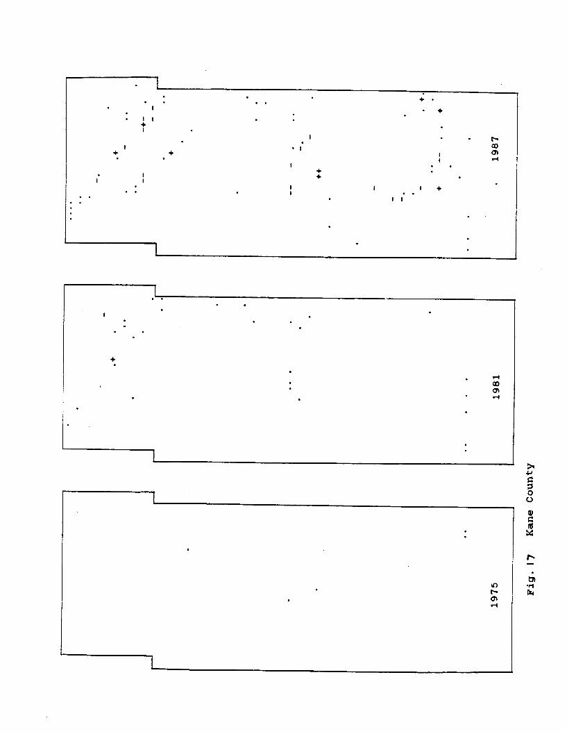
00
t-1
4)
PIO.;;,4J
L

00
(o
*4

S S
* S
*0 * ''65*1
* S
.55
0 *** .*
* . . . S.
t"
T-4
*0
5- 5
* ** S.
.5 S
* 0
,
as!
W-4
1"4<-(
'I
Il
r-(
S . .I
I|
S* *
I
CA
3.,
* I

0.7 0.7
0.34
0.8-
0.7-
0.6a
0.5m
0.4a
0.3a
0.2m
0.1' 0.08
0-'U "l-
2 3
INTERVALS OF4
20 HOURS
Fig. 20. Deer removal rates in 20-hr increments that were achieved bysharpshooters at O'Hare Airport during winter, 1988.
0.15
OOM%
0
I-0
v)wLtw
L&J!Iw:
0 -f-5 6
wa

3d
Xco
0
>-
C
TID
0)6N
N
0
a
0
tO 0 U')F') F') N
o O 0NHS 3- 3 -
0'N0
-0
0
O-Co 0)
O
0
*0
m
0w N 9-li ff 9I TI I v wJ i It . i -
0
1,4
*t444
0
-6
"mo
S'4
Ct
w*o
*ONN3N8sxYVM 8S

0(M
-J
0
0 In it
LJ-J
Li.CN
W-
-a
U..
Sj
li-e
q.44
9'U'
A6
5,49"t-*
0
0 -
..
"0 U
r54
0
NseC
40P 4po
CN

xC
(D~C
(aI' rH~4
I'
I-
o in 0 InN WM V-
a3ddVWi 3A17 330 40 'ON
a00g0
000000000
000
0
00
0000
0
U)
I-0zC-
aa
00
U7.i
O4
*fox
0'
-40
4so
1;
0AFas l<1 ,--
r.M U-
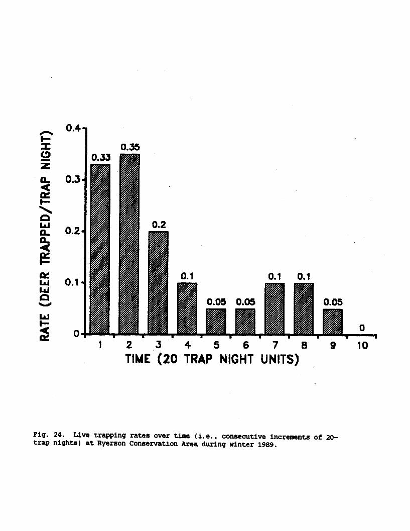
a-
ce,z0..
--
Q..
I.-
lAJFLd
LUI--
T
U.4 4
0.3.
0.2-
0.1.-
0.05 0.05
I F1
0.05
w.1 2 3 4 5 6 7
TIME (20 TRAP NIGHT UNITS)
0UY
8 9 10
Fig. 24. Live trapping rates over time (i.e., consecutive increments of 20-trap nights) at Ryerson Conservation Area during winter 1989.
0.350.33
0.1
A
0.1 0.1
0O
0.2
I 'ITI" To

0
0
x
0
U
0
0
0!0I
6NI~m
00
0
a 00N
in O
ON
o0
aN
0
N314SS)HVl Aa JIOHS
a
0
*.
461
0400
54
em
*s '
In
z
833C! J0 "ON
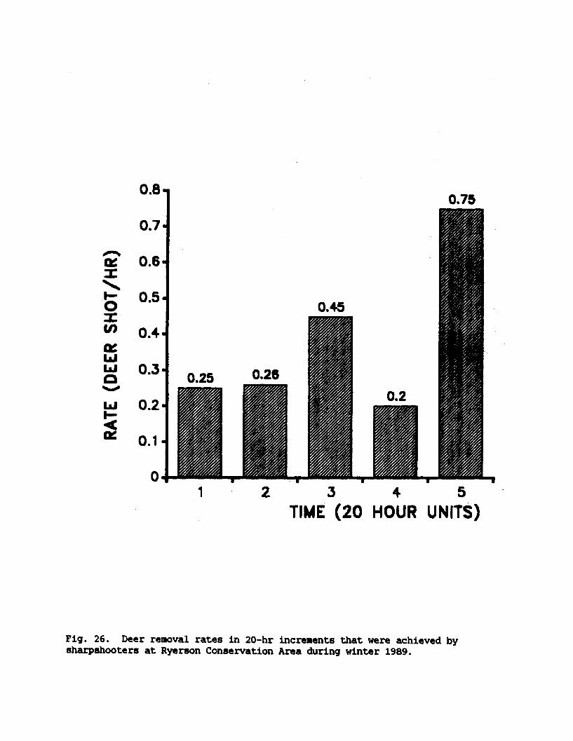
0.75
0.45
0.25 0.26
0.7a
0.6-
0.5.
0.4-
0.3-
0.2-
0.1.
*-*1 2
-ir
3 4 5TIME (20 HOUR UNITS)
"I
Fig. 26. Deer removal rates in 20-hr increments that were achieved bysharpshooters at Ryerson Conservation Area during winter 1989.
0.2
I-.-.
0
I-"La
1ý
0o-
r% a-
mw "row
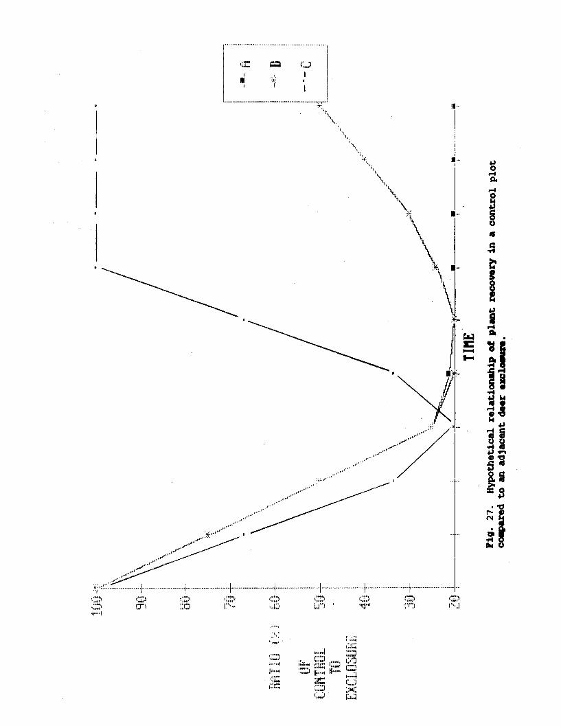
4J0
r-4f-
D0
4
i-
'±1
4ii
"3
. ........ ........... .. .............
ft•ill'
;;:Iie4~
U
I * * .4
......... ...... .........„.. .... ................ ,I
l,,,l'"t
S1.....4 :
:-1#;; 80`so Mee
I. ..... ..............U-1 it: ............................... .... I ...................................... 4......-
.11 1 "0 f. 3.1.1 .1 t. 10, '.4'1M'
II
0l|I-
[*"'.....
I
".... D:
I1

Appendix A. Witham, J.H., and J.M. Jones. 1990. White-tailed deer abundance
on metropolitan forest preserves during winter in northeastern Illinois.
Wildl. Soc. Bull. 18:13-16.

Wildl. Soc. Bull. 18:13-16, 1990
WHITE-TAILED DEER ABUNDANCE ON METROPOLITANFOREST PRESERVES DURING WINTER IN
NORTHEASTERN ILLINOIS
JAMES H. WITHAM, Illinois Natural History Survey, 607 E. Peabody, Champaign, IL 61820
JON M. JONES,' Illinois Natural History Survey, 607 E. Peabody, Champaign, IL 61820
Urban development has expanded beyondthe traditional core areas of most major cities.Land-use planners in many metropolitan areashave recognized the value of natural areas foropen space and have included them as part ofdevelopment schemes (McHarg 1969, Henchet al. 1987, Adams and Dove 1989). These nat-ural areas provide habitat for wildlife as wellas recreational opportunities for people, there-by increasing the occurrence and diversity ofwildlife-human interactions (Bird 1986).
The white-tailed deer (Odocoileus virginia-nus) is the largest wild mammal to inhabit suchnatural areas in the Chicago Metropolitan Area(CMA) of northeastern Illinois. Principal deerhabitat in the CMA is in forest preserves ad-ministered by county governments. The manydeer that inhabit metropolitan forest preserves,coupled with the progressive insularity of thesesites, have led to negative interactions withhumans and to locally severe browsing damageto vegetation. For many CMA residents, thecumulative effects of deer-human conflicts haveexceeded the residents' willingness to toleratesuch damage (Witham and Jones 1987).
We studied white-tailed deer in the CMAfor 5 years, 1984-1988. A substudy objectivewithin this program was to determine the min-imum number of deer on selected metropoli-tan forest preserves during winter.
STUDY AREA AND METHODS
The CMA of Cook, DuPage, and Lake counties en-compasses 4,521 km2 in northeastern Illinois with ahuman population in 1986 of 6.3 million (Table 1).
' Present address: Illinois Dep. of Conservation, 524S. Second Street. Springfield, IL 62706.
Intermixed on this human-dominated landscape are393 km2 of forest preserves representing 8.7% of thetotal CMA. These preserves are discontinuous in dis-tribution and vary in size and degree of insularity.Vegetation and land-use within forest preserves arediverse and range from extensive recreational develop-ments to inviolate natural areas (Wendling et al. 1981).
Swink and Wilhelm (1979) documented species, as-sociations, and distributions of plants in the Chicagoregion. In general, the combination of fire suppressionand succession has led to preserves dominated by oak/maple/basswood (Quercus spp./Acer spp./Tilia amer-icana) forests of mixed types (i.e., mesic upland, dry-mesic upland, bottomland, and flatwoods). Old-fieldsuccessional communities, meadows, and regularlymowed recreational fields are interspersed in and aroundwoodlots. Remnant swamp, marsh, bog, fen, and prai-rie communities also persist (Schwegman 1973:11-14,Wendling et al. 1981).
We defined individual preserves by contiguity ofproperty irrespective of administrative divisions. Un-fenced roads that dissected preserves were not treatedas boundaries. Areal measurements of sizes of individ-ual preserves in DuPage and Lake counties were pro-vided by their forest preserve districts. Sizes of pre-serves in Cook County were determined with a dotgrid overlaid on forest preserve maps. No adjustmentswere made for nondeer habitat (i.e., surface water,roads, and maintenance buildings) within preserves.
Deer were counted from a Cessna 172 fixed-wingaircraft during 1984-1985 and from a Bell Long-Rang-er helicopter during 1985-1988. The helicopter wasfavored because of greater maneuverability and im-proved safety while flying at low altitudes (90-150 mAGL) and reduced speeds (50-60 knots) over devel-oped areas and near major airports. Areas with vege-tative cover that was relatively homogeneous were sur-veyed systematically by flying parallel transectsdetermined by aircraft instrumentation and visualground references. Transect widths were not measured,but we estimate that they varied from 100 m in matureforests to 300 m for agricultural fields without standingcrops. We divided smaller preserves, and areas withheterogeneous vegetative cover types, into subunits withboundaries that were defined by natural features (e.g.,changes in vegetation, rivers, lakes) and roads that werevisible from the air; we searched these subunits sys-tematically and then totaled all nonduplicate deercounted within each preserve. Individual preserves weresurveyed -51 time annually and from 1 to 5 times

14 Wildl. Soc. Bull. 18(1) 1990
Table 1. Chicago Metropolitan Area: human population, and area and size of forest preserves by county.
Counties
Cook DuPage Lake All
Human population ( x 106)' 5.3 0.7 0.3 6.3County area (km2)b 2,454.5 860.1 1,205.9 4,520.5Forest preserve area (km 2 ) 267.9 72.3 52.6 392.8Percent of county in forest preservec 10.9 8.4 4.4 8.7
a 1 July 1986 estimate, US. Census Bureau. released December 1987.b Suburban fact book, 1973, Northeast Illinois Planning Commission, Chicago.c 1 January 1988.
during the study. Surveys were conducted during win-ter when snow depth exceeded 10 cm. Two observersin verbal contact counted deer from I side of the air-craft.
Our counts reflect the maximum number of inde-pendent observations of deer that we made on each
.. site at the time of the census only. We deleted obser-vations where duplicate sightings may have occurred.These included deer that were disturbed by the aircraftand traveled into areas yet to be surveyed. Most deerobserved during surveys remained stationary or moved<50 m toward cover or other deer. Because manyfactors preclude counting all deer on a site, we referto data based on our counts as,"minimum" numbersor "minimum" densities.
RESULTS
The 52 preserves that were surveyed duringthe 5-year period included 93% (366 km2 ) ofthe total forest preserve area in the CMA. Un-surveyed preserves were either small, with fewif any deer present, or were located whereaerial survey access conflicted with airport flightpatterns. Individual preserves ranged from 0.21to 34.37 km 2. The majority (79%, n = 41) ofpreserves in the CMA were < 10 km 2; however,preserves >10 km 2 represented 62% of thetotal area surveyed (Table 2).
We observed deer on 43 of the preserves.Among the 9 preserves where deer were notobserved, all were <2.0 km 2 in size and col-lectively were <3% of the total area of thepreserves surveyed.
Minimum densities of deer on the 52 pre-serves ranged from 0 to 26 deer/km2. How-ever, deer distribution was typically patchy,with animals often concentrated within pre-serves on sites of 1 to 3 km 2 at densities >40
deer/km2 . Minimum densities of deer on 16preserves (33% of all preserves) exceeded 8deer/km2 on at least one survey; 13 (31% ofthe area surveyed) of these sites had > 12 deer/km 2; 7 (14% of the area surveyed) preserveshad 220 deer/km2 (Table 2).
DISCUSSION
We experienced problems in conducting ae-rial flights over the CMA that would not haveoccurred in less developed areas. Airspace wasrigidly controlled by airport control towers.Thirteen pilots were. used in this study; all werecompetent, but varied greatly in their atten-tion to detail and enthusiasm. Pilots experi-enced stress caused collectively by intense con-centration necessary to detect other aircraft inthe congested airspace of the CMA, complexcommunications with air traffic controllers,presence of residential and commercial build-ings, and flight at low altitudes that requiredstandardization and precision to count deer.Because emergency medical service (EMS) isthe priority mission of state-owned helicopters,deer counts were sometimes aborted in flightbecause of EMS requests. Collectively, thesefactors, among others, contributed to our de-cision early in the study to conduct only directcounts of deer.
Direct counts produce limited informationon the distribution of deer, minimum abun-dance, and minimum density. Populationtrends cannot be inferred from these data andlow numbers of deer observed on a site are of

METROPOLITAN DEER ABUNDANCE * Witham and Jones
Table 2. Number of white-tailed deer counted duringaerial surveys on individual forest preserves in the Chi-cago Metropolitan Area conducted during winters,1984-1988. Counts represent the minimum number ofdeer on a preserve during each respective survey only.
Area ofpreserve
(km2)
0.210.700.800.850.981.011.011.091.141.241.241.371.581.681.992.102.102.152.232.252.383.003.143.244.384.404.534.594.695.185.185.415.625.3725.836.246.797.047.208.699.84
10.9514.84.15.3115.7016.0318,8020.9021.6624.8432.0434.37
Number of deer cou
1984 1985 1986
00000
0
00
0110
69
1172
190 1401 2
0 1
23 133 0
9 613 23
14
37 3420 30
35 46
26296
8 22230
10171
74 21)3 253
4047 SS8
35 38
29
63
73136191126.53
682003331017,3
Range ofminimum
inted deerSdensities
1987 1988 (deer/kin)
0 0 0000
2 2 0-26 6
022 20
00
22 180
13 31 7-201 17 0-1
0 040 19
01 0
15 75 2
5-100-1
69 222-33-5
13 12 397 21
7-84-6
11 15 0-342 61 6-13
44 825 33 4-621 19 3-519 17 1-3
1-322 13 2-3
0 9 0-187 10-1317 221 7-22
18 103 7-20!81 18-26
4-6
135 73
372 6-178-13
40 138 3-5o-
value as distributional records only. However,the documentation of high minimum deerdensities is important to metropolitan landmanagers who must prioritize their deer man-agement activities among the expansive pre-serves that exist within the CMA. Deer den-sities observed in the CMA suggest thatmanagers should be concerned in at least 13of the 52 preserves surveyed. Those 13 pre-serves represent 114 km 2 (31%) of the total areaof forest preserves in the CMA.
Our conservative counts of deer are re-markable primarily because they indicate anextensive distribution of large numbers of deeracross a major metropolitan landscape with highhuman densities. The abundance of deer inthe CMA is a direct result of historic land-usedecisions, which preserved habitat sanctuaries(Forest Preserve District of Cook County 1918)on the periphery of a major city that continuedto expand. Deer abundance is dynamic, andthe location and severity of site-specific con-flicts are already diverse and will continue tochange over time. The extensive distributionof forest preserves and the large number thatinterface private and municipal properties inthe CMA will require the development of site-specific evaluations with clearly defined deermanagement objectives. Some will require in-tensive management, but in others greater ac-ceptance or tolerance of damages caused bylarge numbers of deer may be necessary.
Acknowledgments.-We thank G. C. San-derson, W. R. Edwards, and A. Hodgins of theIllinois Natural History Survey for their re-views of the manuscript. This study is a con-tribution of Federal Aid in Wildlife Restora-tion Project W-87-R, the Illinois Departmentof Conservation, the U.S. Fish and WildlifeService, and the Illinois Natural History Sur-vey, cooperating.
LITERATURE CITED
ADAMS. L. W.. AND L. E. DOVE. 1989. Wildlife re-serves and corridors in the urban environment.Natl. Inst. for Urban Wildl., Columbia, Md. 91pp.1530 1
15
f:
q
16 Wildl. Soc. Bull. 18(1) 1990
BIRD. D. M. 1986. City critters: how to live with urbanwildlife. Eden Press, Montreal, Canada. 128pp.
FOREST PRESERVE DISTRICT OF COOK COUNTY. 1918.Forest preserves of Cook County, Illinois, 1914-1918. Clohesey and Company Printers, Chicago.145pp.
HENCH, J. E., K. VAN NESS, AND R. GIBBS. 1987. De-velopment of a natural resources planning andmanagement process. Pages 29-35 in L. W. Adamsand D. L. Leedy, eds. Integrating man and naturein the metropolitan environment. Natl. Inst. forUrban Wildl., Columbia, Md.
McHARG, I. L. 1969. Design with nature. NaturalHistory Press, Garden City, N.Y. 197pp.
SCHWEGMAN, J. E. 1973. Comprehensive plan for theIllinois Nature Preserves System, Part 2, The nat-ural divisions of Illinois. 11. Nat. Pres. Comm.,Springfield. 32pp.
SWINK, F., AND G. S. WILHELM. 1979. Plants of theChicago region. Third ed. The Morton Arboretum,Lisle, I11. 922 pp.
WENDLING, R. C., S. J. GABRIEL, J. F. DWYER, AND R.L. BucK. 1981. Forest Preserve District of CookCounty, Illinois. J. For. 79:602-605.
WrrHAM, J. H., AND J. M. JONES. 1987. Deer-humaninteractions and research in the Chicago metro-politan area. Pages 155-159 in L. W. Adams andD. L. Leedy, eds. Integrating man and nature inthe metropolitan environment. Natl. Inst. for Ur-ban Wildl., Columbia, Md.
Received 4 May 1989.Accepted 24 August 1989.

Appendix B. Watkins, B.E., J.H. Witham, D.E. Ullrey, D.J. Watkins, and J.M.
Jones. 1991. Body composition and condition of white-tailed deer fawns. J.
Wildl. Manage. 55:39-51.

BODY COMPOSITION AND CONDITION EVALUATION OFWHITE-TAILED DEER FAWNS
BRUCE E. WATKINS,' Chicago Zoological Society, Brookfield Zoo, Brookfield, IL 60513JAMES H. WITHAM, Illinois Natural History Survey, 607 E. Peabody Street, Champaign, IL 61820DUANE E. ULLREY, Department of Animal Science, Michigan State University, E. Lansing, MI 48824DEBORAH J. WATKINS,' Chicago Zoological Society, Brookfield Zoo, Brookfield, IL 60513JON M. JONES,2 Illinois Natural History Survey, 607 E. Peabody Street, Champaign, IL 61820
Abstract: Sixteen white-tailed deer (Odocoileus virginianus) fawns were captured between November andApril 1984-86 near Chicago, Illinois, to evaluate relationships between body composition and conditionindices. Body fat (bled, ingesta-free basis) of the fawns ranged from 2.3 to 48.9%, dry-matter basis. Of 6morphometric indices, chest girth had the highest correlations with body mass, gross energy, and fat. Of 45postmortem indices, carcass mass and composition, viscera mass and composition, Kistner score, kidney fatmass, and gastrocnemius protein had the highest correlations with body mass and composition. Kidney fatindices, kidney fat mass, and back fat thickness were related to body fat concentration by logarithmicfunctions. Kistner score and gastrocnemius fat concentration were each linearly related to body fat concen-tration. Femur marrow fat and mandible marrow fat concentrations were each related to the negative inverseof body fat concentration. Serum triiodothyronine had the closest relationships with body energy contentand body fat concentration of the 11 blood and serum constituents we analyzed. Multiple regression analysisindicated that body gross energy content could best be predicted in live fawns by a combination of live massand triiodothyronine and postmortem by a combination of viscera mass and live mass or gastrocnemius fatmass, kidney fat mass and kidney mass, or gastrocnemius fat mass and liver mass.
J. WILDL MANAGE. 55(1):39-51
Accurate assessment of body condition ofwhite-tailed deer is essential for understandingthe interactions that occur between deer pop-ulations and their environment and, in turn, forsuccessful management. Although extensive lit-erature is available on ungulate condition in-dices (Kirkpatrick 1980, Franzmann 1985), fewattempts have been made to determine rela-tionships between indices and the attributes theyare intended to reflect (Robbins 1983:222).
Condition indices related to (1) body massand morphometry, (2) body composition, and(3) metabolic status have received widespreadattention in white-tailed deer. Commonly-usedgravimetric and morphometric indices includelive mass, dressed-carcass mass, and various lin-ear and circumferential measurements (e.g.,Smart et al. 1973, Roseberry and Klimstra 1975,Weckerly et al. 1987). Commonly-used bodycomposition indices include bone marrow fatconcentration, the kidney fat index (KFI), andvisual scoring methods (e.g., Ransom 1965, Ba-ker and Leuth 1966, Kistner et al. 1980). Indi-cators of metabolic status include blood urea
I Present address: Durango Software, P.O. Box 2783,Durango, CO 81302.
2Present address: Illinois Department of Conser-vation, 524 S. Second Street, Springfield, IL 62706.
nitrogen, serum nonesterified fatty acids(NEFA), and triiodothyronine (T3) (e.g., Kirk-patrick et al. 1975, Seal et al. 1978, Bahnak etal. 1981). We believe all 3 types of indices arerequired for accurate condition assessment, be-cause body mass, body composition, and met-abolic status can have dynamic interrelation-ships, i.e., different body compositions for thesame body mass, and vice versa, or differentmetabolic states for the same body mass andcomposition. For example, fawns with restrictedfood intake or fed a poor quality diet can ac-cumulate substantial fat reserves during autumneven though their body mass is reduced (Vermeand Ozoga 1980a,b; Watkins 1980). An indexrelated only to body fat concentration might notbe sufficiently sensitive to differentiate thesefawns from larger, well-nourished fawns.
Our objective was to determine how variousindices were related to body size, body com-position, and metabolic status of white-taileddeer fawns. We thank P. Whetter, M. E. Keeffe,J. W. Seets, R. Dobbins, G. Sanderson, and W.Edwards for their assistance. Our research wassupported by the Illinois Natural History Sur-vey, with contributions from the Federal Aid inWildlife Restoration Project (W-87-R), the Il-linois Department of Conservation, and the U.S.Fish and Wildlife Service.
39

40 DEER CONDITION EVALUATION * Watkins et al.
METHODSBetween November and April 1984-86, 16
white-tailed deer fawns (10 M, 6 F) were cap-tured by rocket net on county forest preservesnear Chicago, Illinois. Two deer were collectedin November, 4 in December, 2 in January, 7.in March, and 1 in April. Immediately aftercapture, animals were manually restrained, agedas fawns based on the absence of the third molar,sampled for blood by jugular puncture, and eu-thanized by injection of T-61 solution (NationalLaboratories, Somerville, N.J.).
Body ProcessingThe fawns were transported from the field to
a laboratory and processed within 1 hour afterdeath. Each animal was weighed and measuredas described by Feldhamer et al. (1985), exceptthat right shoulder height was measured fromthe plantar surface of the hoof. Animals werebled from the neck over a tared polyethylenebag and eviscerated. Contents of the digestivetract (ingesta) were removed, and urine con-tained in the bladder was discarded. The skinwith hair and dew claws intact (hide) was care-fully removed with a minimum of adherentmuscle and fat. Carcass fat, musculature, andvisceral fat were visually scored (Kistner et al.1980). The thyroid lobes were removed andtrimmed to remove extraneous tissue. The M.gastrocnemius muscle from the point of inser-tion of the tendon of Achilles to the points oforigin on the lateral and medial heads of thefemur was removed from the right leg. Marrowplugs (about 3 cm long) were taken from thecenter of the right femur and from the centerof the right mandible. The heart was removedfrom the pericardium and sliced to removeblood. The kidneys were removed along withall adherent fat and weighed. In very fat ani-mals, fat associated with the kidney was differ-entiated from that associated with the perito-neum based on the most obvious discontinuity.Perirenal fat was trimmed as described by Riney(1955), and the mass of the kidney and remain-ing fat was determined. The kidney was thendecapsulated and weighed. We calculated kid-ney fat masses (including the mass of the fibrouscapsule) based on total and trimmed perirenalfat. Kidney fat masses were not obtained for 3animals. Two kidney fat indices were calculatedfor each kidney and for both kidneys combined:total KFI = (total kidney fat mass x 100)/kid-
ney mass; trimmed KFI = (trimmed kidney fatmass x 100)/kidney mass. An index (Conindex)based on fresh femur fat concentration and lefttrimmed KFI was calculated following Con-nolly (1981:334). Back-fat thickness was deter-mined by making a cut perpendicular to thebackbone just caudal to the last sacral vertebraand measuring fat depth (mm) at the thickestpoint.
The trachea, larynx, diaphragm, esophagus,and all contents of the pleural and peritonealcavities exclusive of ingesta were combined (vis-cera). All other tissues exclusive of the visceraand hide were combined (carcass). Mass of theblood drained from the neck, blood and fluidfrom the pleural and peritoneal cavities, bloodretained in the heart, and blood obtained byvenipuncture (blood) was determined for 14 ofthe deer.
Body components <6 kg were weighed to thenearest 0.1 g; body components a6 kg wereweighed to the nearest gram. All tissues weredouble-bagged in air-tight polyethylene linersand stored at -20 C until ground or analyzed.Carcass (exclusive of the gastrocnemius, thy-roids, and marrow plugs), viscera, and hide wereground twice with a large, auger grinder with1-cm plate openings. Random samples (about1.2 kg carcass and viscera, and about 0.2 kg hide)of the mixed, ground tissues were placed in tared,aluminum pans, bagged, and frozen at -20 Cfor chemical analysis. Gastrocnemius muscleswere ground twice with a table-top auger grind-er and frozen at -20 C for chemical analysis.
Blood samples obtained by venipuncture wereplaced on ice immediately after collection andthen refrigerated at approximately 7 C. After20-24 hours, blood in nonheparinized tubes wascentrifuged, and serum was collected. Serumsamples were stored at -23 C until analyzed.Blood collected in heparinized tubes was re-frigerated for 20-24 hours until hematologicalanalyses were performed.
Analytical MethodsBlood and tissue samples were freeze-dried
and ground in a blender into homogeneousmixtures. Dry matter, gross energy, crude pro-tein, fat, and ash were determined as describedby McCullough and Ullrey (1983). Serum sam-ples were analyzed for NEFA following Falholtet al. (1973), for urea nitrogen (SUN) with acommercial diacetylmonoxine procedure (Sig-ma Chemical Co., St. Louis, Mo.), and for pro-
J. Wildl. Manage. 55(1):1991

DEER CONDITION EVALUATION * Watkins et al. 41
tein with a refractometer. Serum thyroxine (T4)was measured as described by Watkins et al.(1983). Serum T3 was determined with a solid-phase radioimmunoassay (Gammacoat, ClinicalAssays, Travenol-Genentech Diagnostics, Cam-bridge, Mass.) validated for deer serum (T3 re-covery = 105.6 ± 2.4 [SE]; parallelism [expect-ed-observed ng/mL]: 0.57-0.54, 1.14-1.12; 2.85at serum volume used in assay, 5.7-5.4, 9.12-7.51). Hematocrit (PCV) was determined withmicrocapillary tubes, and hemoglobin (Hgb) wasmeasured by the cyanomethemoglobin method.Red blood cell counts (RBC) were made with aCoulter Counter. Mean erythrocyte cell volume(MCV), mean corpuscular hemoglobin (MCH),and mean corpuscular hemoglobin concentra-tion (MCHC) were calculated with standard for-mulas.
Statistical MethodsWe used the SPSS/PC+ statistical program
(Norusis 1988:B-197-B-243) to analyze bodycomposition (Y,) relationships with each index(Xa,) and sex (X,2) (0 = M, 1 = F) based on thefollowing model:
Y, = Bo + BX,, + B2 X, 2 + B 3X,~X, 2 + e,.
When B, and B3 did not differ significantly (P_ 0.05) from zero based on a partial F-test, a
bivariate model was used. When necessary, de-pendent and/or independent variables weretransformed to achieve linearity. We selectedthe transformation providing the highest cor-relation coefficient with the most normal andindependent distribution of residuals. Signifi-cance for regressions was considered to be P <
0.05. Forward multiple regression analysis wasperformed on normal and transformed data todetermine if the inclusion of more than 1 indexvariable would significantly (P s 0.05) improvethe regression. A paired t-test was used to testfor differences between the right and left kid-neys.
Body Composition BasisMass and chemical composition of the body
were expressed on 3 bases by summing all bodycomponents exclusive of (1) ingesta (unbled.body); (2) blood and ingesta (body); and (3) hide,blood, and ingesta (skinned body). Statisticalanalyses were performed with each basis as thedependent variable. Results are presented on abled, ingesta-free basis unless major differencesoccurred among the bases or another basis was
considered relevant. All concentrations are pre-sented on a dry matter basis unless a fresh massbasis is indicated.
RESULTSLive masses of the 16 fawns ranged from 16.8
to 41.6 kg, and body fat varied from 2.3 to 48.9%(Table 1). Blood had little influence on overallbody composition with all body chemical com-ponents highly correlated (r > 0.99) with re-spective unbled body components. Most modelsfor predicting body composition had slightlyhigher correlations when the skinned body wasused as the basis.
Relationships with Body MassCarcass, live, and gastrocnemius masses had
the highest correlations with body mass (Table2). Kidney masses were only moderately relatedto body mass (Table 3). Of the morphometricindices, chest girth showed the highest corre-lations with live and body masses. Males tendedto have greater body mass than females for agiven hindfoot length (P = 0.19) or total bodylength (P = 0.12).
Relationships with Body ComponentConcentrations
Carcass and viscera gross energy and fat con-centrations had the highest correlations withbody gross energy and fat concentrations (Table4). Kistner score also was highly correlated withbody gross energy concentration (Fig. 1).
Indices correlated (r > 0.9) with percent bodyfat and best described by simple linear rela-tionships were Kistner Score, Conindex, and gas-trocnemius fat. Indices correlated (r > 0.9) withbody fat by logarithmic functions included totalkidney fat mass, total KFI (Fig. 2), trimmedKFI, and back fat. Females tended to have ahigher total kidney fat mass than males for agiven body fat concentration (0.08 < P < 0.17).Relative to body fat concentration, females hadhigher right total KFI values than males (P =0.03). Combined total KFI (P = 0.07) and lefttotal KFI (P = 0.18) also tended to be relativelyhigher in females. Differences in total or trimmedKFI values between the right and left kidneyswere not significant. Indices correlated (r > 0.9)with body fat concentration by exponentialfunctions included femur marrow dry matter(%), fresh femur marrow fat (%), mandible mar-row dry matter (%), and fresh mandible marrowfat (%).
J. Wildl. Manage. 55(1):1991

42 DEER CONDITION EVALUATION * Watkins et al.
Table 1. Characteristics of white-tailed deer fawns from northern Illinois, November-May 1984-86.
Characteristic' n t SE Range
Live mass (kg) 16 31.1 2.0 16.8-41.6Total body length (cm) 16 141.7 2.1 129.0-156.0Chest girth (cm) 16 75.5 0.1 69.0-81.0
Bled, ingesta-free bodyMass (kg) 16 26.9 2.3 12.9-38.0Dry matter (%) 16 36.9 1.6 29.4-47.0Crude protein (%) 16 57.0 3.6 39.2-75.5Fat (%) 16 24.5 4.7 2.3-48.9Ash (%) 16 13.8 1.4 6.7-23.0Gross energy (meal) 16 62.7 9.2 15.5-115.4Gross energy (mcal/kg) 16 5.63 0.27 4.0-7.0
Hide (kg) 16 2.1 0.1 1.3-3.1Viscera (kg) 16 4.2 0.4 1.9-6.4Carcass (kg) 16 20.4 1.5 9.3-28.5Ingesta (kg) 14 2.8 0.2 1.7-5.1
Right M. gastrocnemiusMass (g) 16 232.5 16.1 90.0-312.3Dry matter (%) 16 25.6 0.5 23.0-29.1Crude protein (%) 16 80.6 1.5 73.4-94.2Fat (%) 16 6.8 1.0 1.3-11.6Gross energy (mcal/kg) 16 5.50 0.05 5.1-5.8
KidneysMass (g) 14 75.1 5.1 44.9-111.9Total fat mass (g) 13 113.7 37.4 3.1-363.0Total kidney fat index 13 253.2 83.8 10.0-842.0
Kistner score 16 40.0 8.2 0.0-90.0Triiodothyronine (ng/mL) 16 1.32 0.22 0.1-2.8
a All concentrations are on a dry matter basis.
When expressed on a dry matter basis, femurmarrow fat (Fig. 3) and mandible marrow fatconcentrations were best related to body fat us-ing a - 1/Y transformation. Examination of theserelationships revealed that dry femur and man-dible fat concentrations exceeding 87 and 75%,
respectively, were not significantly related tobody fat. Below 87 and 75%, femur fat andmandible fat concentrations were related to bodyfat percent by exponential models: In(Bodyfat[%]) = 0.0136(Femur fat[%] + 0.958, r = 0.92,n = 7, SE = 0.216; In(Body fat[%]) =
Table 2. Significant (P s 0.0001) bivariate regression models with body mass as the dependent variable for white-tailed deerfawns from northern Illinois, November-May 1984-86.
SE ofIndependent variable Dependent variable' Intercept Slope r estimate n
Carcass mass (g) Live mass (kg) 5.390 0.0013 0.993 0.94 16Gastrocnemius mass (g) Live mass (kg) 4.210 0.1160 0.952 2.47 16Chest girth (mm) Live mass (kg) -66.400 0.1350 0.916 3.25 16Live mass (kg) Unbled body mass (kg) -4.980 1.0600 0.996 0.83 14Carcass mass (g) Body mass (kg) -0.223 0.0013 0.995 0.85 16Live mass (kg) Body mass (kg) -5.640 1.0470 0.994 0.94 16Gastroenemius mass (g) In(Body mass) (kg) 2.080 0.0050 0.967 0.09 16In(Viscera mass) (g) In(Body mass) (kg) -3.060 0.7610 0.944 0.11 16
In(Hide mass) (g) Body mass (kg) -182.900 27.6000 0.933 3.06 16In(Liver mass) (g) Body mass (kg) -153.200 28.4000 0.932 2.68 12
Chest girth (mm) Body mass (kg) -76.600 0.1430 0.923 3.27 16
In(Heart mass) (g) Body mass (kg) -160.400 33.1000 0.921 3.32 16
Live mass (kg) Skinned body mass (kg) -5.580 0.9780 0.994 0.91 16
a Body mass - mass of the bled, ingesta-free body.
J. Wildl. Manage. 55(1):1991

DEER CONDITION EVALUATION * Watkins et al. 43
Table 3. Index relationships (r : 0.9) with bled, ingesta-free body mass and composition of white-tailed deer fawns from northernIllinois, November-May 1984-86. P < 0.05 unless indicated by NS (i.e., nonsignificant).
Dependent variablea
Body mass (kg)
Body gross energy(mcal/kg)
Body fat (%)
Body crude protein(%)
Body gross energy(meal)
Body fat (g)Body crude protein
(g)Body ash (g)
Independent variableb (r) (model type]
Total kidney mass (0.88) [1]; Right kidney mass (0.88) [1]; Total body length (0.85)[1]; Shoulder height (0.81) [1]; Hindfoot length (0.76) [1]; Blood mass (0.70) [3];Left kidney mass (0.68) [1]; Thyroid mass (0.63) [3]; Ingesta mass (NS).
Live mass (0.87) [4]; Gastrocnemius GE (kcal/g) (0.83) [3]; Blood GE (kcal/g)(0.77) [3]; Hide GE (kcal/g) (0.66) [3]
Mandible marrow fat (%) (0.89) [5]; Live mass (0.87) [4]; Hide fat (%) (0.83) (2]; T3(0.82) [1]; MCHC (-0.79) [6]; chest girth (0.74) [4]; SUN (-0.63) [4]; RBC (0.63)[3]; PCV (0.62) [3]; T4 (0.62) [3]; Serum protein (0.60) [3]; Blood fat (%) (NS);NEFA (NS); Hbg (NS); MCH (NS); MCV (NS).
Gastrocnemius crude protein (%) (0.82) [2]; Live mass (-0.80) [1]; Hide crude pro-tein (%) (NS).
Gastrocnemius mass (0.88) [4]; chest girth (0.83) [1]; T3 (0.75) [1]; MCHC (0.75) [6];RBC (0.69) [3]; PCV (0.67) [3]; T4 (0.66) [3]; Serum protein (0.63) [3]; SUN(-0.54) [4]; Hgb (0.52) [3]; NEFA (NS); MCH (NS); MCV (NS).
Hide mass (0.88) [1]; Chest girth (0.79) [4].Hide mass (0.87) [1]; Liver mass (0.87) (3]; Total kidney mass (0.84) [1] Viscera
mass (0.81) [11Total body length (0.8) [1]. Hindfoot length (0.66) [1]; Chest girth (0.65) [1]; Car-
cass mass (0.64) [1]; Live mass (0.6) [1]; Shoulder height (0.58) [11
a Body concentrations are on a dry matter basis.b GE - gross energy; Hgb - hemoglobin (g/dL); MCH - mean corpuscular hemoglobin (pg/RBC); MCHC - mean corpuscular hemoglobin
concentration (g/dL cells); MCV = mean corpuscular volume (fL); NEFA - serum nonesterifed fatty acids (/un/L); PCV - packed cell volume(%); RBC - red blood cell count (10
6/mm3); SUN - serum urea nitrogen (mg/dL); T3 - serum triiodothyronine (ng/mL); T4 - serum thyroxine
(ng/mL).c Model type: [1] Y - Bo + BiX; (2] Y - Bo + Biln(X); (3] In(Y) - Bo + BIX; [4] I(Y) - Bo + BIln(X), [5] Y - -l/(Bo + BiX); [6] Y - Bo +
BiX + B2(Sex).
0.016(Mandible fat[%]) + 0.848, r = 0.79, n =7, SE = 0.035).
Carcass and viscera crude protein concentra-tions were highly related to body crude proteinby linear relationships. Gastrocnemius crudeprotein concentration provided the next best in-dex to body crude protein.
Serum T3 showed the closest relationship withbody fat of the blood and serum constituents weanalyzed. Sex interacted with mean corpuscular
'8
If
7.5.
7.0-
6.5-
6.0-
5.5-
5.0-
4.51
4.04
3.5-
300-
Y= 0.033)( + 4.32 r = 0.97
U ^
I I I I I I I I I I0 10 20 30 40 50 60 70 80 90 100
Ktner ScoreFig. 1. The relationship between bled, ingesta-free body grossenergy (kcal/g, dry basis) and Kistner score (Kistner et al. 1980)for white-tailed deer fawns from northern Illinois, November-April 1984-86.
hemoglobin concentration as a predictor of bodyfat (P = 0.02). Serum protein values tended tobe higher relative to body fat in females thanmales (P = 0.06).
Relationships with Body ComponentQuantities
Body gross energy (mcal) was most closelyrelated to viscera mass (kg) (Fig. 4). Kistner
Y = 10.18W(nX) - 13.25
UaL
r= 0.98
U U 10UU 1U 20J z 0U uu 35oU 40 45U
Rigt Tota Kidney Fat IndexFig. 2. The relationship between bled, ingesta-free body fat(%, dry basis) and right kidney fat index based on total perirenalfat for white-tailed deer fawns from northern Illinois, Novem-ber-April 1984-86.
J. Wildl. Manage. 55(1):1991
CA
I• ,.v-1 :A
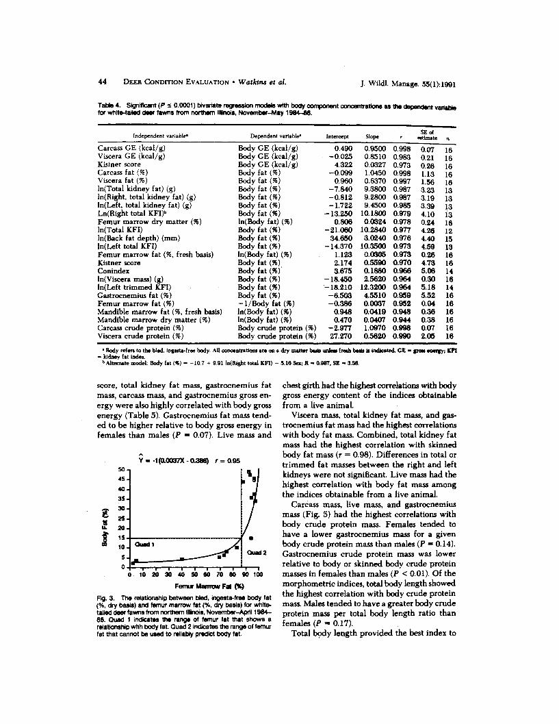
44 DEER CONDITION EVALUATION * Watkins et al.
Table 4. Significant (P :s 0.0001) bivariate regression models with body component concentrations as the dependent variablefor white-tailed deer fawns from northern Illnois, November-May 1984-86.
SE ofIndependent variable
" Dependent variable' Intercept Slope r estimate n
Carcass GE (kcal/g) Body GE (kcal/g) 0.490 0.9500 0.998 0.07 16Viscera GE (kcal/g) Body GE (kcal/g) -0.025 0.8510 0.983 0.21 16Kistner score Body GE (kcal/g) 4.322 0.0327 0.973 0.26 16Carcass fat (%) Body fat (%) -0.099 1.0450 0.998 1.13 16Viscera fat (%) Body fat (%) 0.960 0.6370 0.997 1.56 16In(Total kidney fat) (g) Body fat (%) -7.840 9.3800 0.987 3.23 13In(Right, total kidney fat) (g) Body fat (%) -0.812 9.2800 0.987 3.19 13ln(Left, total kidney fat) (g) Body fat (%) -1.722 9.4500 0.985 3.39 13Ln(Right total KFI)b Body fat (%) -13.250 10.1800 0.979 4.10 13Femur marrow dry matter (%) ln(Body fat) (%) 0.806 0.0324 0.978 0.24 16In(Total KFI) Body fat (%) -21.060 10.2840 0.977 4.26 12ln(Back fat depth) (mm) Body fat (%) 34.650 3.0240 0.976 4.40 15ln(Left total KFI) Body fat (%) -14.370 10.3500 0.973 4.59 13Femur marrow fat (%, fresh basis) ln(Body fat) (%) 1.123 0.0305 0.973 0.26 16Kistner score Body fat (9) 2.174 0.5590 0.970 4.73 16Conindex Body fat (%) 3.675 0.1880 0.966 5.06 14ln(Viscera mass) (g) Body fat (9) -18.450 2.5620 0.964 0.30 16ln(Left trimmed KFI) Body fat (%) -18.210 12.3200 0.964 5.18 14Gastrocnemius fat (%) Body fat (%) -6.503 4.5510 0.959 5.52 16Femur marrow fat (%) -1/Body fat (9) -0.386 0.0037 0.952 0.04 16Mandible marrow fat (%, fresh basis) ln(Body fat) (%) 0.948 0.0419 0.948 0.36 16Mandible marrow dry matter (%) ln(Body fat) (%) 0.470 0.0407 0.944 0.38 16Carcass crude protein (%) Body crude protein (%) -2.977 1.0970 0.998 0.07 16Viscera crude protein (%) Body crude protein (9) 27.270 0.5620 0.990 2.05 16
a Body refers to the bled, ingesta-free body. All concentrations are on a dry matter basis unless fresh basis is indicated. GE - gross energy; KFI= kidney fat index.
b Alternate model: Body fat (%) - -10.7 + 9.91 ln(Right total KFI) - 5.16 Sex; R - 0.987, SE - 3.38.
score, total kidney fat mass, gastrocnemius fatmass, carcass mass, and gastrocnemius gross en-ergy were also highly correlated with body grossenergy (Table 5). Gastrocnemius fat mass tend-ed to be higher relative to body gross energy infemales than males (P = 0.07). Live mass and
Y = -1(0.00037X - 0.386) r = 0.95
L.
0 10 20 30 40 50 60 70 80 90 100
Femur Marrow Fal (%)
Fig. 3. The relationship between bled, ingesta-free body fat(%, dry basis) and femur marrow fat (%, dry basis) for white-tailed deer fawns from northern Illinois, November-April 1984-86. Quad 1 indicates the range of femur fat that shows arelationship with body fat. Quad 2 indicates the range of femurfat that cannot be used to reliably predict body fat.
chest girth had the highest correlations with bodygross energy content of the indices obtainablefrom a live animal.
Viscera mass, total kidney fat mass, and gas-trocnemius fat mass had the highest correlationswith body fat mass. Combined, total kidney fatmass had the highest correlation with skinnedbody fat mass (r = 0.98). Differences in total ortrimmed fat masses between the right and leftkidneys were not significant. Live mass had thehighest correlation with body fat mass amongthe indices obtainable from a live animal.
Carcass mass, live mass, and gastrocnemiusmass (Fig. 5) had the highest correlations withbody crude protein mass. Females tended tohave a lower gastrocnemius mass for a givenbody crude protein mass than males (P = 0.14).Gastrocnemius crude protein mass was lowerrelative to body or skinned body crude proteinmasses in females than males (P < 0.01). Of themorphometric indices, total body length showedthe highest correlation with body crude proteinmass. Males tended to have a greater body crudeprotein mass per total body length ratio thanfemales (P = 0.17).
Total body length provided the best index to
J. Wildl. Manage. 55(1):1991
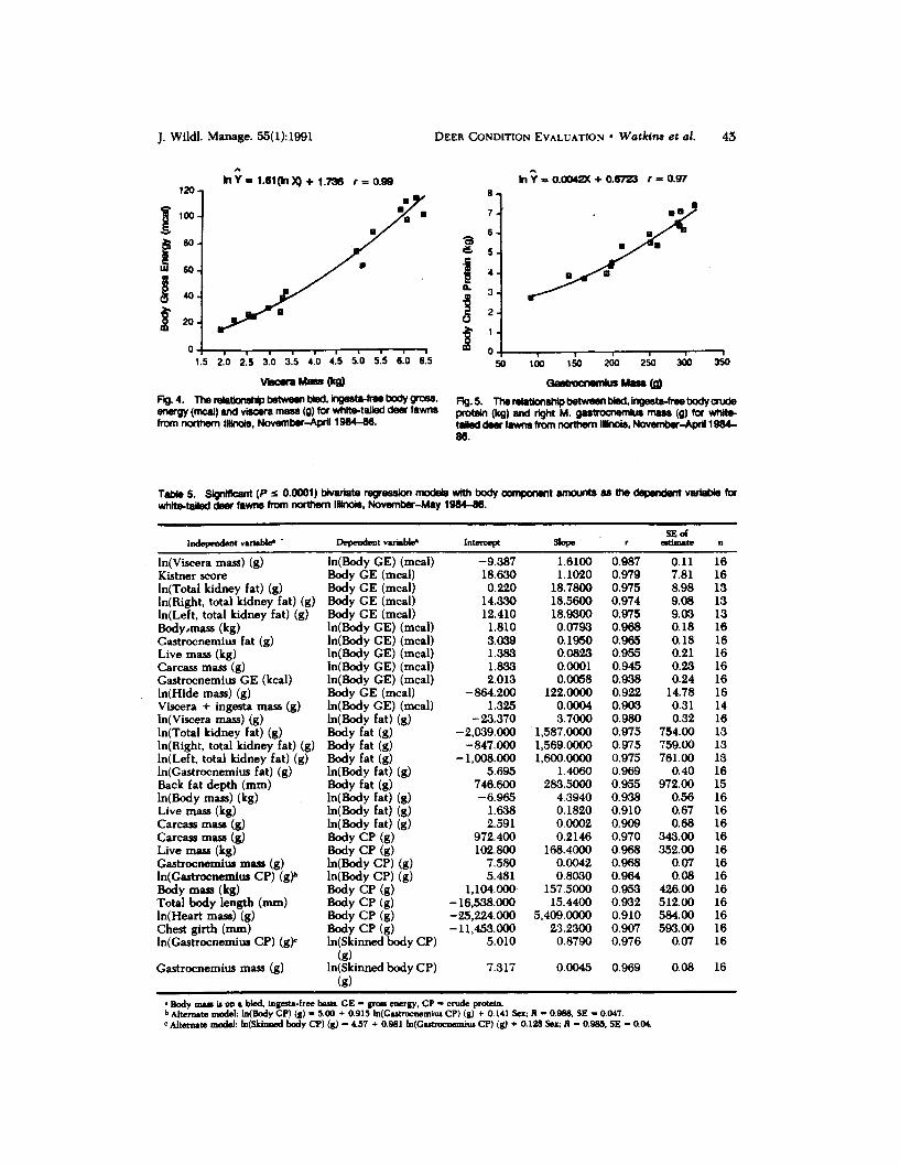
DEER CONDITION EVALUATION * Watkins et al. 45
120.
100-
80 -
40.oS20-
In Y 1.61(In X) + 1.736 r = 0.998.
7.
6.'8I~, 5.I
4.0,
1.5 2.0 2.5 3.0 3.5 4.0 4.5 5.0 5.5 6.0 6.5
Viscera Ma (kg)
Fig. 4. The relationship between bled, ngesta-free body gross,energy (mcal) and viscera mass (g) for white-tailed deer fawnsfrom northern Illinois, November-April 1984-86.
YIn = 0.0042)X+0.6723 r = 0.97
a gs"
---- I--- | -- I --- I --- I ---
50 100 150 200 250 300 350
Gastomemnius Mass (g)
Fig. 5. The relatonshp between bled, ngesta-free body crudeprotein (kg) and right M. gastrocnemlus mass (g) for white-tailed deer fawns from northern llinois, November-Apr1984-86.
Table 5. Significant (P s 0.0001) bivarilate regression models with body component amounts as the dependent variable forwhite-tailed deer fawns from northern Ilinois, November-May 1984-86.
SE ofIndependent variable* " Dependent variables Intercept Slope r estimate n
In(Viscera mass) (g) ln(Body GE) (meal) -9.387 1.6100 0.987 0.11 16Kistner score Body GE (meal) 18.630 1.1020 0.979 7.81 16ln(Total kidney fat) (g) Body GE (meal) 0.220 18.7800 0.975 8.98 13In(Right, total kidney fat) (g) Body GE (meal) 14.330 18.5600 0.974 9.08 13ln(Left, total kidney fat) (g) Body GE (meal) 12.410 18.9300 0.975 9.03 13Bodymass (kg) ln(Body GE) (meal) 1.810 0.0793 0.968 0.18 16Gastrocnemius fat (g) ln(Body GE) (meal) 3.039 0.1950 0.965 0.18 16Live mass (kg) ln(Body GE) (meal) 1.383 0.0823 0.955 0.21 16Carcass mass (g) ln(Body GE) (meal) 1.833 0.0001 0.945 0.23 16Gastrocnemius GE (kcal) ln(Body GE) (meal) 2.013 0.0058 0.938 0.24 16ln(Hide mass) (g) Body GE (meal) -864.200 122.0000 0.922 14.78 16Viscera + ingesta mass (g) ln(Body GE) (meal) 1.325 0.0004 0.903 0.31 14ln(Viscera mass) (g) In(Body fat) (g) -23.370 3.7000 0.980 0.32 16ln(Total kidney fat) (g) Body fat (g) -2,039.000 1,587.0000 0.975 754.00 13In(Right, total kidney fat) (g) Body fat (g) -847.000 1,569.0000 0.975 759.00 13ln(Left, total kidney fat) (g) Body fat (g) -1,008.000 1,600.0000 0.975 761.00 13ln(Gastrocnemius fat) (g) In(Body fat) (g) 5.695 1.4060 0.969 0.40 16Back fat depth (mm) Body fat (g) 746.600 283.5000 0.955 972.00 15In(Body mass) (kg) ln(Body fat) (g) -6.965 4.3940 0.938 0.56 16Live mass (kg) ln(Body fat) (g) 1.638 0.1820 0.910 0.67 16Carcass mass (g) In(Body fat) (g) 2.591 0.0002 0.909 0.68 16Carcass mass (g) Body CP (g) 972.400 0.2146 0.970 343.00 16Live mass (kg) Body CP (g) 102.800 168.4000 0.968 352.00 16Gastrocnemius mass (g) ln(Body CP) (g) 7.580 0.0042 0.968 0.07 16ln(Gastrocnemius CP) (g)b ln(Body CP) (g) 5.481 0.8030 0.964 0.08 16Body mass (kg) Body CP (g) 1,104.000 157.5000 0.953 426.00 16Total body length (mm) Body CP (g) -16,538.000 15.4400 0.932 512.00 16ln(Heart mass) (g) Body CP (g) -25,224.000 5,409.0000 0.910 584.00 16Chest girth (mm) Body CP (g) -11,453.000 23.2300 0.907 593.00 16ln(Gastrocnemius CP) (g)c In(Skinned body CP) 5.010 0.8790 0.976 0.07 16
(g)Gastrocnemius mass (g) In(Skinned body CP) 7.317 0.0045 0.969 0.08 16
(g)a
Body mass is on a bled, ingesta-free basis. GE gross energy, CP - crude protein.b Alternate model: ln(Body CP) (g) - 5.00 + 0.915 ln(Gastrocnemius CP) (g) + 0.141 Sex; R - 0.988, SE - 0.047.c
Alternate model: In(Skinned body CP) (g) - 4.57 + 0.981 In(Gastrocnemius CP) (g) + 0.128 Sex; R - 0.985, SE = 0.04.
J. Wildl. Manage. 55(1):1991
v I"a .4I l lV I IvIi I I -I- -I •

46 DEER CONDITION EVALUATION * Watkins et al.
body ash mass. Live mass and body mass werepoor predictors of body ash mass.
Serum T3 concentration showed the closestrelationship with body gross energy content ofthe blood and serum constituents we analyzed.Sex interacted with mean corpuscular hemoglo-bin concentration as a predictor of body grossenergy (P = 0.04). Serum protein values tendedto be higher relative to body gross energy infemales than males (P = 0.06).
Multiple Regression ModelsIn live animals, live mass and T3 were the
most useful variables for predicting body grossenergy content and body fat concentration withmultiple regression models (Table 6). Regres-sions for predicting body gross energy (meal) inlive animals were significantly improved by in-cluding Hgb and mean corpuscular hemoglobinconcentration. These models were recalculatedwith Hgb and mean corpuscular hemoglobinconcentration eliminated because of the ques-tionable value of the hematological values. Post-mortem, viscera mass, live mass, gastrocnemiusfat mass, Kistner score, total kidney fat mass,kidney mass, and liver mass were useful forpredicting body gross energy (mcal).
Comparing aggregate profiles of blood andserum constituents to body fat or gross energyhad little advantage over using individual con-stituents. Multiple regression analysis indicateda combination of T3 and serum protein provid-ed the best prediction of body fat concentrationand body gross energy (meal).
DISCUSSIONBody Mass Indices
It is often impractical to weigh deer in thefield. In our study, chest girth provided the bestpremortem prediction of live mass. Our modelfor predicting live mass from chest girth has asteeper slope than models presented by Weck-erly et al. (1987) for fawns in Tennessee. In-cluding very fat and very lean animals in oursample might account for this difference. Car-cass mass and gastrocnemius mass appear to beuseful indices for predicting body mass post-mortem.
Indices of Body ComponentConcentrations
Since the 1940's, femur marrow fat has beenused widely as an ungulate condition index. Toeliminate errors that might result from desic-
cation before analysis, femur fat concentrationis often expressed on a dry matter basis. Ourdata indicate that femur fat (dry matter basis)has limited usefulness as an index because it isnot mobilized by fawns until body fat declinesto about 15%. The body fat concentration of thefawns in our sample having >87% femur fatcould not be differentiated based only on femurfat concentration; e.g., a fawn having 15% bodyfat could have the same percentage of femurfat as a fawn having 49% body fat. Below 87%femur fat, large differences in femur fat con-centrations reflected only small differences inbody fat concentrations.
Mandible marrow fat concentration has beenreported to reflect a wider range of body fatthan percent femur fat (Baker and Lueth 1966)and to separate deer into more distinguishablecondition classes (Nichols and Pelton 1974).Mandible marrow also can be collected moreeasily from hunter-killed animals. From our re-sults, mandible fat offers no advantage over fe-mur fat for predicting body fat concentrationin white-tailed deer. Femur fat and mandiblefat concentrations are highly correlated, and therelationship between mandible fat and body fatis basically the same, although weaker, as thatfor femur fat. Mandible fat was not mobilizedby the fawns until body fat declined to approx-imately 12%. The body fat concentrations offawns in our sample having >75% mandible fatcould not be differentiated based only on man-dible fat concentration.
Because of its predictable relationship withmarrow fat concentration, marrow dry matterpercentage, as determined by oven-drying orreagent methods (Neiland 1970, Verme andHolland 1973), is sometimes used instead of etherextraction for estimating the fat concentrationof marrow. Our results suggest that marrow drymatter concentration, particularly for the fe-mur, might actually be a better index of bodyfat concentration than marrow fat percentage.Similar to marrow fat, marrow dry matter con-centration cannot be used to discriminate amonganimals with a high body fat concentration.However, the less curvilinear relationship ob-served between femur marrow dry matter andbody fat suggests that body fat concentrationsup to approximately 30% might be accuratelypredicted with femur dry matter concentrationsup to 80%. These relationships would be appli-cable only to fresh marrow samples that havenot desiccated prior to analysis.
Unlike the exponential relationships shown by
J. Wildl. Manage. 55(1):1991

J. Wildl. Manage. 55(1):1991
E0z
C
+
+
Of
Iq
?i
A
~
0
a
a
0.5U
0
.0
.5
0A0
fl'
C
BQ
a
DEER CONDITION EVALUATION * Watkins et al. 47
!SS8§ooooo=o smooS
Od-^lddddddt'dOddcd
9 8- 0 X -X --8X"C -M8t-t--
P-4 P" o=4~
CO e 00q 0000to 00t
do dd0d ddoddddddd
O- I
OOOO^^^CtOOMO OOca 8 00 cz V --qC 000 0 0 OOCl-t- o eqN c q - oe -
CO) qvC5C 5 O o lO 00tr- co) Z P eqc -i C4t--. ci P-*6 ddd do id
^^ C'^»»^-^<C|O OccOO f0O
2 E
'^codd ^-ddd -ibirddd
G3^*S i'5 ^' 51(z Q 0000 00 eq L LO c co11 g~ s6 6o 6 6 L6 ^~^i
> >
c^O ^O- IIO IC'OCOODI 4
I I < I'- I I
COO ov cS 3 0 N^M~ Sc (M 2.i cIV v P4 Uj cý3-84 Lcl q 6cioCý 6c ýF4 ( dL - ~
C
e
-g
"2
g-a2
U|
1z
||A
^' A
S31'-
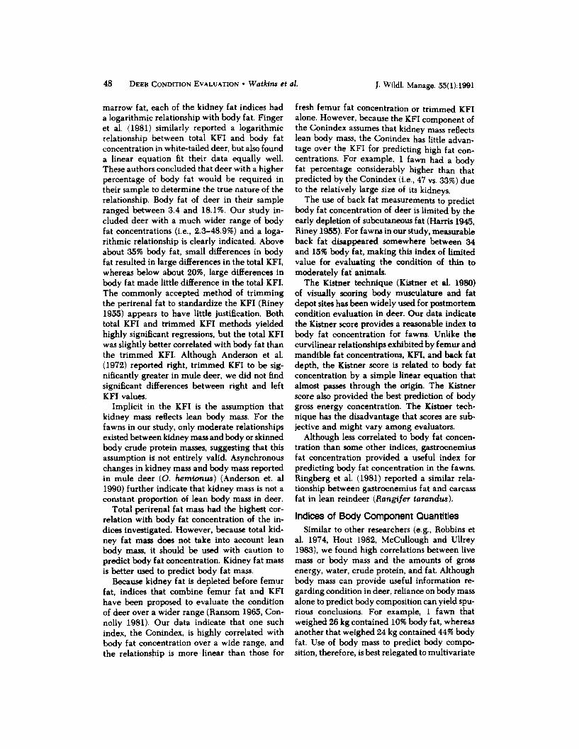
48 DEER CONDITION EVALUATION * Watkins et al.
marrow fat, each of the kidney fat indices hada logarithmic relationship with body fat. Fingeret al. (1981) similarly reported a logarithmicrelationship between total KFI and body fatconcentration in white-tailed deer, but also founda linear equation fit their data equally well.These authors concluded that deer with a higherpercentage of body fat would be required intheir sample to determine the true nature of therelationship. Body fat of deer in their sampleranged between 3.4 and 18.1%. Our study in-cluded deer with a much wider range of bodyfat concentrations (i.e., 2.3-48.9%) and a loga-rithmic relationship is clearly indicated. Aboveabout 35% body fat, small differences in bodyfat resulted in large differences in the total KFI,whereas below about 20%, large differences inbody fat made little difference in the total KFI.The commonly accepted method of trimmingthe perirenal fat to standardize the KFI (Riney1955) appears to have little justification. Bothtotal KFI and trimmed KFI methods yieldedhighly significant regressions, but the total KFIwas slightly better correlated with body fat thanthe trimmed KFI. Although Anderson et al.(1972) reported right, trimmed KFI to be sig-nificantly greater in mule deer, we did not findsignificant differences between right and leftKFI values.
Implicit in the KFI is the assumption thatkidney mass reflects lean body mass. For thefawns in our study, only moderate relationshipsexisted between kidney mass and body or skinnedbody crude protein masses, suggesting that thisassumption is not entirely valid. Asynchronouschanges in kidney mass and body mass reportedin mule deer (0. hemionus) (Anderson et. al1990) further indicate that kidney mass is not aconstant proportion of lean body mass in deer.
Total perirenal fat mass had the highest cor-relation with body fat concentration of the in-dices investigated. However, because total kid-ney fat mass does not take into account leanbody mass, it should be used with caution topredict body fat concentration. Kidney fat massis better used to predict body fat mass.
Because kidney fat is depleted before femurfat, indices that combine femur fat and KFIhave been proposed to evaluate the conditionof deer over a wider range (Ransom 1965, Con-nolly 1981). Our data indicate that one suchindex, the Conindex, is highly correlated withbody fat concentration over a wide range, andthe relationship is more linear than those for
fresh femur fat concentration or trimmed KFIalone. However, because the KFI component ofthe Conindex assumes that kidney mass reflectslean body mass, the Conindex has little advan-tage over the KFI for predicting high fat con-centrations. For example, 1 fawn had a bodyfat percentage considerably higher than thatpredicted by the Conindex (i.e., 47 vs. 33%) dueto the relatively large size of its kidneys.
The use of back fat measurements to predictbody fat concentration of deer is limited by theearly depletion of subcutaneous fat (Harris 1945,Riney 1955). For fawns in our study, measurableback fat disappeared somewhere between 34and 15% body fat, making this index of limitedvalue for evaluating the condition of thin tomoderately fat animals.
The Kistner technique (Kistner et al. 1980)of visually scoring body musculature and fatdepot sites has been widely used for postmortemcondition evaluation in deer. Our data indicatethe Kistner score provides a reasonable index tobody fat concentration for fawns. Unlike thecurvilinear relationships exhibited by femur andmandible fat concentrations, KFI, and back fatdepth, the Kistner score is related to body fatconcentration by a simple linear equation thatalmost passes through the origin. The Kistnerscore also provided the best prediction of bodygross energy concentration. The Kistner tech-nique has the disadvantage that scores are sub-jective and might vary among evaluators.
Although less correlated to body fat concen-tration than some other indices, gastrocnemiusfat concentration provided a useful index forpredicting body fat concentration in the fawns.Ringberg et al. (1981) reported a similar rela-tionship between gastrocnemius fat and carcassfat in lean reindeer (Rangifer tarandus).
Indices of Body Component QuantitiesSimilar to other researchers (e.g., Robbins et
al. 1974, Hout 1982, McCullough and Ullrey1983), we found high correlations between livemass or body mass and the amounts of grossenergy, water, crude protein, and fat. Althoughbody mass can provide useful information re-garding condition in deer, reliance on body massalone to predict body composition can yield spu-rious conclusions. For example, 1 fawn thatweighed 26 kg contained 10% body fat, whereasanother that weighed 24 kg contained 44% bodyfat. Use of body mass to predict body compo-sition, therefore, is best relegated to multivariate
J. Wildl. Manage. 55(1):1991

DEER CONDITION EVALUATION * Watkins et al.
models that include at least 1 independent vari-able related to fat.
Gastrocnemius fat mass and gross energy (kcal)may provide the most practical single indicesof body gross energy (mcal) even though visceramass, Kistner score, and total kidney fat massshowed stronger relationships. The high corre-lation between viscera mass and body gross en-ergy probably reflected a relationship betweenlean viscera mass and lean body mass, and theimportance of the viscera as a fat storage site.Use of viscera mass as a practical index is limitedby the laborious task of removing the ingesta.Including ingesta mass with the viscera sub-stantially diminished the accuracy of predictingbody gross energy. We do not recommend Kist-ner score as a single index of body gross energycontent because no consideration is made forbody size. Total kidney fat mass should be usedwith caution because its relationship with bodygross energy is highly curvilinear. Using the gas-trocnemius has the advantages that it can becollected in the field with relative ease, gas-trocnemius mass is related to body mass, andthe relationship between body gross energy andgastrocnemius gross energy content is only mod-erately curvilinear.
Viscera mass and total kidney fat mass alsohad the highest correlations with body fat mass.Similar to the prediction of body gross energycontent, the labor required to remove the in-gesta and the highly curvilinear relationship be-tween kidney fat mass and body fat mass limitthe practicality of these indices for predictingbody fat mass. Again, gastrocnemius fat massmight be a more practical index.
Live mass, carcass mass, and gastrocnemiusmass were the most practical single indicatorsof body crude protein mass. Expressing crudeprotein content on a skinned body basis has theadvantage of eliminating the influence of ker-atin proteins from the pelage. Gastrocnemiuscrude protein mass provided the best predictionof skinned body crude protein mass. Ringberget al. (1981) reported a linear relationship be-tween gastrocnemius mass and total muscle massin lean reindeer. In our study, relationships be-tween gastrocnemius mass and body or skinnedbody crude protein mass were slightly exponen-tial, indicating that relatively less body proteinis associated with the gastrocnemius in largeranimals. The lower crude protein content of thegastrocnemius relative to body crude protein infemales may reflect a greater skeletal muscle
mass in males. When it is not possible to obtainlive mass or gastrocnemius mass, total bodylength appears to provide a fair index to bodycrude protein mass.
Metabolic StatusSeveral studies on the effects of diet compo-
sition, food intake, and starvation on blood andserum characteristics of white-tailed deer haveindicated the potential efficacy of serum ureanitrogen, nonesterified fatty acids, and the thy-roid hormones (particularly T3) for discrirni-nating metabolic status (e.g., Seal et al. 1978,Bahnak et al. 1979, Watkins et al. 1982). In ourstudy, serum T3 had the highest correlationswith body fat and gross energy of the blood andserum constituents evaluated. Although T3would appear to be a useful index of metabolicstatus, little is known about the factors that caninfluence this hormone. A negative energy bal-ance can cause serum T3 to decline in white-tailed deer and other animals (Watkins et al.1982). However, in a study of fawns restrictedto 50% of ad libitum intake during the fall, adecrease in serum T3 did not occur even thoughthe growth rate of the restricted fawns was sig-nificantly reduced (Watkins 1980). This suggeststhat during the period of obligate lipid depo-sition, T3 levels will not necessarily decline eventhough fawns are energy-restricted and stuntedin size. In addition, because of the small cir-culating reservoir of T3 and low binding affinityof serum proteins, serum T3 levels might beeasily influenced by short-term perturbations(Watkins et al. 1983).
Most of the other blood and serum constitu-ents showed only moderate relationships withbody fat or gross energy. Serum T4 was lessrelated to body fat than T3. Unlike T3, serumT4 in white-tailed deer is strongly influencedby season (Watkins et al. 1983), and this mayhave partially obscured its relationship with bodycomposition. Serum urea nitrogen was relatedinversely to body fat, indicating that musclecatabolism was fueling an increasing proportionof the energy requirement as body fat concen-tration declined. Serum nonesterified fatty acidswere not related to body fat or gross energy.Responses of serum nonesterfied fatty acids toenergy restriction in captive deer have beeninconsistent (e.g., Seal et al. 1978, Warren et al.1982, Card et al. 1985) suggesting that the fac-tors influencing fatty acids of metabolic originin the blood may be too complex for practical
J. Wildl. Manage. 55(1):1991 49

50 DEER CONDITION EVALUATION * Watkins et al.
value. The reported effects of dietary proteinand/or energy intake on hematological valuesof white-tailed deer have also been conflicting(e.g., Seal et al. 1978, Warren et al. 1982,DelGiudice et al. 1987). These inconsistenciesmake the use of hematological values question-able for condition assessment.
MANAGEMENT IMPLICATIONSCondition Evaluation
Because many relationships between indicesand body composition are not linear, we thinkpredicted body composition rather than indexvalues should serve as the basis for evaluatingthe condition of deer. Predicted body gross en-ergy (meal), within sex and age classes and with-in seasons, would provide the most practical sin-gle basis for evaluating condition. This measuretakes into account body mass and compositionand provides a representation of the amount ofmetabolic fuel available to the animal. Ideally,predicted body gross energy should be used incombination with an index of metabolic status.Although T3 is the most promising metabolicindicator we evaluated, it appears to give onlya very broad indication of metabolic status. Fac-tors independent of diet that might influenceT3 need further study.
The applicability of our data to other ageclasses and to other times of the year is notknown. Additional research is required to es-tablish if indices show similar relationships tobody composition when deer are in an anabolicstate.
Assessing Condition Premortem.-Live massand T3 offer the greatest potential for assessingthe condition of live fawns during winter interms of body gross energy (meal). When it isnot possible to obtain live mass, a combinationof chest girth and T3 appears to provide a fairprediction of body gross energy.
Assessing Condition Postmortem.-A com-bination of viscera mass and live mass or gas-trocnemius fat mass provided the best postmor-tem predictions of body gross energy (meal) inthe fawns. Excluding viscera mass, body grossenergy was best predicted by a combination oftotal kidney fat mass and total kidney mass, orgastrocnemius fat mass and liver mass. As a sin-gle index, the gastrocnemius holds promise as auseful indicator for evaluating the condition ofdeer because it can be collected in the field andused to predict body mass, body gross energy,
body crude protein mass, and body fat mass andconcentration.
LITERATURE CITEDANDERSON, A. E., D. C. BOWDEN, AND D. E. MEDIN.
1990. Indexing the annual fat cycle in a muledeer population. J. Wildl. Manage. 54:550-556.
---- , D. E. MEDIN, AND D. C. BOWDEN. 1972.Indices of carcass fat in a Colorado mule deerpopulation. J. Wildl. Manage. 36:579-594.
BAHNAK, B. R., J. C. HOLLAND, L. J. VERME, AND J.J. OZOGA. 1979. Seasonal and nutritional effectson serum nitrogen constituents in white-taileddeer. J. Wildl. Manage. 43:454-460.
--- ---- , ---- , AND ----. 1981. Sea-sonal and nutritional influences on growth hor-mone and thyroid activity in white-tailed deer.J. Wildl. Manage. 45:140-147.
BAKER, M. F., AND F. X. LEUTH. 1966. Mandibularcavity tissue as a possible indicator of conditionof deer. Proc. Annu. Conf. Southeast Assoc. Gameand Fish Comm. 20:69-74.
CARD, W. C., R. L. KIRKPATRICK, K. E. WEBB, JR.,AND P. F. SCANLON. 1985. Nutritional influ-ences on NEFA, cholesterol, and ketones in white-tailed deer. J. Wildl. Manage. 49:380-385.
CONNOLLY, G. E. 1981. Assessing populations. Pages287-345 in 0. C. Wallmo, ed. Mule and black-tailed deer of North America. Univ. NebraskaPress, Lincoln.
DELGIUDICE, G. D., L. D. MECH, U. S. SEAL, ANDP. D. KARNS. 1987. Effects of winter fastingand refeeding on white-tailed deer blood profiles.J. Wildl. Manage. 51:865-873.
FALHOLT, K., B. LUND, AND W. FALHOLT. 1973.An easy colorimetric micromethod for routinedetermination of free fatty acids in plasma. Clin.Chem. Acta 46:105-111.
FELDHAMER, G. A., J. R. STAUFFER, JR., AND J. A.CHAPMAN. 1985. Body morphology and weightrelationships of Sika deer in Maryland. Z. Sau-getierkunde 50:88-106.
FINGER, S. E., I. L. BRISBIN, M. H. SMITH, AND F. D.URBSTON. 1981. Kidney fat as a predictor ofbody condition in white-tailed deer. J. Wildl.Manage. 45:964-968.
FRANZMANN, A. W. 1985. Assessment of nutritionalstatus. Pages 239-259 in R. J. Hudson and R. G.White, eds. Bioenergetics of wild herbivores. CRCPress, Inc., Boca Raton, Fla.
HARRIS, D. 1945. Symptoms of malnutrition in deer.J. Wildl. Manage. 9:319-322.
HOUT, J. 1982. Body condition and food resourcesof white-tailed deer on Anticosti Island, Quebec.Ph.D. Thesis, Univ. Alaska, Fairbanks. 240pp.
KIRKPATRICK, R. L. 1980. Physiological indices inwildlife management. Pages 99-112 in S. D.Schemnitz, ed. Wildlife management techniquesmanual. Fourth ed. The Wildlife Society, Wash-ington, D.C.
, D. E. BUCKLAND, W. A. ABLER, P. F.SCANLON, J. B. WHELAN, AND H. E. BURKHART.
1975. Energy and protein influences on bloodurea nitrogen of white-tailed deer fawns. J. Wildl.Manage. 39:692-698.
J. Wildl. Manage. 55(1):1991

DEER CONDITION EVALUATION * Watkins et al. 51
KISTNER, T P , C. E. TRAINER, AND N. A. HARTMANN.1980. A field technique for evaluating physicalcondition of deer. Wildl. Soc. Bull. 8:11-17.
McCULLOLGH, D. R.. AND D. E. ULLREY. 1983.Proximate mineral and gross energy compositionof white-tailed deer. J. Wildl. Manage. 47:430-441.
NEILAND, K. A. 1970. Weight of dried marrow asindicator of fat in caribou femurs. J. Wildl. Man-age. 34:904-907.
NICHOLS, R. G., AND M. R. PELTON. 1974. Fat inthe mandibular cavity as an indicator of condi-tion in deer. Proc. Annu. Conf. Southeast. Assoc.Game and Fish Comm. 28:540-548.
NoRusIS, M. J. 1988. SPSS/PC + V2.0 base manual.SPSS Inc., Chicago, 11. 60 6 pp.
RANSOM, A. B. 1965. Kidney and marrow fat asindicators of white-tailed deer condition. J. Wildl.Manage. 29:397-398.
RINEY, T. 1955. Evaluating condition of free-rang-ing red deer (Cervus elaphus) with special ref-erence to New Zealand. N.Z. J. Sci. and Technol.36:429-463.
RINGBERG, T. M., R. G. WHITE, D. F. HOLLEMAN,AND J. R. LUICK. 1981. Prediction of carcasscomposition in reindeer (Rangifer tarandus tar-andus L.) by use of selected indicator bones andmuscles. Can. J. Zool. 59:583-588.
ROBBINS, C. T. 1983. Wildlife feeding and nutri-tion. Academic Press, New York, N.Y. 343pp.
--- , A. N. MOEN, AND J. T. REID. 1974. Bodycomposition of white-tailed deer. J. Anim. Sci.38:871-876.
ROSEBERRY, J. L., AND W. D. KLIMSTRA. 1975. Somemorphological characteristics of the Crab Or-chard deer herd. J. Wildl. Manage. 39:48-58.
SEAL, U. S., L. J. VERME, AND J. J. OZOGA. 1978.Dietary protein and energy effects on deer fawnmetabolic patterns. J. Wildl. Manage. 42:776-790.
SMART, C. W., R. H. GILES, JR., AND D. C. GUYNN,JR. 1973. Weight tape for white-tailed deer inVirginia. J. Wildl. Manage. 37:553-555.
VERME, L. J., AND J. C. HOLLAND. 1973. Reagent-dry assay of marrow fat in white-tailed deer, J.Wildl. Manage. 37:103-105.
----- , AND J. J. OZOGA. 1980a. Influence of pro-tein-energy intake on deer fawns in autumn. J.Wildl. Manage. 44:305-314.
---- , AND . 1980b. Effects of diet ongrowth and lipogenesis in deer fawns. J. Wildl.Manage. 44:315-324.
WARREN, R. J., R. L. KIRKPATRICK, A. OELSCHLAE-GER, P. F. SCANLON, K. E. WEBB, JR., AND J. B.WHELAN. 1982. Energy, protein, and seasonalinfluences on white-tailed deer fawn nutritionalindices. J. Wildl. Manage. 46:302-312.
WATKINS, B. E. 1980. Iodine status and thyroidactivity of white-tailed deer (Odocoileus virgi-nianus borealis). Ph.D. Thesis, Michigan StateUniv., E. Lansing. 119pp.
--- , R. F. NACHREINER, S. M. SCHMITT, T. M.COOLEY, AND D. E. ULLREY. 1982. Thyroidfunction in fed and fasted white-tailed deer fawns.Can. J. Zool. 60:1331-1338.
---- , D. E. ULLREY, R. F. NACHREINER, AND S.M. SCHMrrITT. 1983. Effects of supplemental io-dine and season on thyroid activity of white-tailed deer. J. Wildl. Manage. 47:45-58.
WECKERLY, F. W., P. L. LEBERGý AND R. A. VANDEN BUSSCHE. 1987. Variation of weight andchest girth in white-tailed deer. J. Wildl. Manage.51:334-337.
Received 16 June 1989.Accepted 14 September 1990.Associate Editor: Morrison/Lancia.
J. Wildl. Manage. 55(1): 1991

Appendix C. Watkins, B.E., J.H. Witham, and D.E. Ullrey. 1992. Body
composition changes in white-tailed deer fawns during winter. Can. J. Zool.
00:000-000 (in press).

Body composition changes in white-tailed deer fawns during winter
Bruce E. Watkins1
Chicago Zoological Society, Brookfield Zoo, Brookfield., IL,
U.S.A. 60513
James H. Witham
Illinois Natural History Survey, 607 E. Peabody. Champaign.
IL. U.S.A. 61820
Duane E.
Department of Animal Science,
East Lansing. MI
Ullrey
Michigan State University.
U.S.A. 48824
Please address correspondence to: Dr. Bruce E. Watkins, P.O. Box 2783,
Durango, CO, U.S.A. 81302 (303) 247-4871
IPresent address: Durango Software, P.O. Box 2783, Durango, CO,
U.S.A. 81302.
4. mbf w ý fý4t M.a 6
Watkins 2
Watkins, B. E., Witham, J. H., and Ullrey, D. E. 1991. Body composition
changes in white-tailed deer fawns during winter. Can. J. Zool. 00:
000-000.
Body composition was determined for 16 white-tailed deer
(Odocoileus virginianus) fawns captured near Chicago, Illinois between
November and April to investigate changes in body composition and
chemical component distribution as fawns catabolized tissues over the
winter. Live weights of the fawns ranged from 16.8 to 41.6 kg, and
ether-extractable fat concentration of the bled, ingesta-free body ranged
from 2.3 to 48.9%, dry basis. Carcass, viscera, and hide contained, on
average, 70%, 21%, and 9% of the bled, whole body fat, respectively.
Above approximately 15% whole body fat (dry basis), the percentage of
body fat in the viscera increased and the percentage in the carcass
declined. Body composition (blood-, ingesta-, and fat-free basis)
averaged 72% water, 23% crude protein, and 5% ash; ash and phosphorus
concentrations increased and protein concentration decreased over the
winter. Sodium concentration tended to decrease. Based on relationships
between chemical components and body weight, the composition of weight
lost during winter was calculated to range from 12% water, 84% fat, 4%
protein, and 0.5% ash during early winter to 73% water, 0.3% fat, 25%
protein, and 2% ash during early spring. Calculated metabolizable energy
derived from tissue catabolism was a quadratic function of body weight
and ranged from 7.7 to 1.1 Mcal/kg of bled, ingesta-free weight loss
during early and late periods.

Watkins
Introduction
Knowledge of body composition is important for evaluating the
condition of deer and for understanding the effects of environmental
factors on deer populations. White-tailed deer in northern latitudes
normally undergo seasonal anabolic-catabolic cycles with concomitant
changes in body composition. In a study of white-tailed deer in Quebec,
Hout (1982) found seasonal differences not only in fat content but also
in fat-free body composition. Most studies on the body composition of
white-tailed deer (Robbins et al. 1974, McCullough and Ullrey 1983,
Rumpler et al. 1987) have not investigated seasonal changes.
Net tissue catabolism by deer is critical for winter survival when
food quantity and quality are inadequate. Few attempts have been made to
determine the composition of winter weight loss in deer. Based on
relationships between body composition and body weight in white-tailed
deer fawns during winter, Hout (1982) concluded that body protein and ash
losses were relatively constant at 22% and 3-4% of weight lost,
respectively, whereas the rates of fat catabolism and water loss
decreased and increased, respectively, as fawns lost weight. Using
isotope dilution, Torbit et al. (1985) reported protein losses accounted
for 20-34% of the body energy catabolized by captive mule deer (Q.
hemionous) during winter. Also using isotope dilution, Delgiudice et al.
(1990) reported weight lost by adult, captive white-tailed deer averaged
24% water, 56% fat, 18% protein, and 3% ash.
Our objectives were (1) to investigate changes in body composition
and chemical component distribution as fawns underwent net catabolism
during the winter, and (2) to calculate the composition and energy

Watkins 4
content of lost weight based on changes in body composition with
decreasing weight.
Methods
Sixteen free-ranging white-tailed deer fawns (10 males, 6 females)
were captured by rocket net near Chicago, Illinois between 1984 and 1986
during late November (N - 2), December (N - 4), January (N - 2), March (S
- 7), and early April (N - 1). Each animal was immobilized with a
combination of ketamine hydrochloride and xylazine hydrochloride (Watkins
et al. 1990a), sampled for blood by jugular venipuncture, and
euthanized by injection of T-61 solution (Watkins et al. 1982). Animals
were processed as described by Watkins et al. (1990b). The animals were
bled from the neck over a tared container and then eviscerated. The
contents of the stomach, intestines, and cecum were removed and weighed
(ingesta). The hide, including skin, hair, and dewclaws, was removed
with a minimum of adherent fat and muscle. The M. gastrocnemius muscle
was removed from the right leg, the heart was removed from the
pericardium, kidneys were decapsulated and weighed without perirenal fat,
and thyroid gland lobes were trimmed of fat. All contents of the pleural
and peritoneal cavities, exclusive of ingesta, were combined with the
trachea, larynx, esophagus, diaphragm, and thyroid glands (viscera). All
tissues exclusive of the hide and viscera were combined (carcass).
Tissues were double-bagged in air-tight polyethylene liners and stored at
-20 C until ground twice using a large, auger-type grinder. Tissue and
blood samples were freeze-dried and analyzed as described by McCullough
and U11rey (1983). Fat was determined by extraction with diethyl ether
and protein was calculated by multiplying Kjeldahl nitrogen by 6.25.

Watkins 5
Blood, ingesta, kidney, liver, and thyroid weights were not determined
for 2 animals (a female in November, and a male in April). Blood
analyses were not available for 2 other animals.
For analysis, the fawns were divided into two groups: those
captured early (i.e., November-January; 6 males, 2 females) and those
captured late (i.e., March and April; 4 males, 4 females). An
independent t-test was used to test for differences in body composition
and component distribution between periods. Data were analyzed with
males and females combined and for males only. Regression analysis was
performed using SPSS/PC+ statistical software (Norusis 1988). The
following model was used to determine relationships between body
components (Yj and Xji) and sex (Xi2; 0 - male, 1 - female):
Yi " Bo _0 BAIX + B2Xi2 + 3X2Xiz+ + ei.
When B2 and B3 did not differ significantly (P < 0.05) from zero based on
a partial F-test, a bivariate model was used. When necessary, dependent
and/or independent variables were transformed to achieve linearity. The
transformation providing the highest correlation with the most normal and
independent distribution of residuals was selected. Significance for all
analyses was considered to be P < 0.05.
The composition of weight loss was estimated by (1) using
regression analysis to determine the relationships between chemical
component weights and bled, ingesta-free body (BIFB) weight, (2)
differentiating the equations obtained in step 1 to determine rates of
component loss (g) per kg of BIFB loss, (3) standardizing the rates of
total component loss to equal 1 kg (i.e., individual component loss/total
component loss x 1000), and (4) using regression analysis to determine

Watkins 6
the rates of standardized component loss relative to BIFB weight. Six
fawns (early period: 3 males, 1 female; late period: 1 male, 1 female)
were omitted from the analysis because they did not follow a pattern of
decreasing fat concentration with decreasing body weight.
Gross energy (GE) and metabolizable energy (ME) were calculated
from fat (i.e., ether extract) and protein (i.e., crude protein) using
coefficients of 9.5 kcal GE per g of fat, 5.65 kcal GE per g of protein,
9 kcal ME per g of catabolized fat, and 4.4 kcal ME g of catabolized
protein (based on a nitrogen-correction factor of 7.45 kcal/g of urinary
nitrogen). The mean BIFB GE of the fawns calculated using coefficients
was 61.4 Mcal versus 62.7 Mcal determined by bomb calorimetry.
Results
Body Weight Relationships
Live and BIFB weights of the fawns ranged from 27-41.6 and 23.8-38
kg, respectively, during the early period and from 16.8-31.1 and 12.9-
26.4 kg during the late period (Table 1). Body and body component
weights generally decreased between periods whereas the weight of stomach
contents increased. Viscera weight decreased relative to BIFB weight but
relative liver, kidney, and thyroid weights did not change between
periods. Heart and gastrocnemius weights increased relative to BIFB
weight but not relative to fat-free BIFB weight.
Blood weight (g) was moderately related to IFB weight (kg):
[1] In Blood weight - 0.73(In IFB wt) + 4.64, r - 0.72, SEE - 0.24.
Ingesta weight was not related to IFB weight (P - 0.9).
Fat. Protein, and Mineral Distribution

Watkins
BIFB fat, dry matter basis (DMB), varied from 34-48.9% during the
early period and from 2.3-15% during the late period (Table 2). On the
average, carcass, viscera, and hide contained 69.7% + 2.4, 21% + 2, and
9.3% + 2.9 of the BIFB fat, respectively. As BIFB fat (DMB) increased up
to approximately 15%, the percentage of BIFB fat contributed by the
carcass increased, the percentage contributed by the viscera remained
fairly constant (14.1% + 0.7, N - 8), and the percentage contributed by
the hide decreased (Fig. 1). Above approximately 15% BIFB fat (DMB) the
percentage of BIFB fat contributed by the carcass gradually decreased,
the percentage contributed by viscera gradually increased, and the
percentage contributed by the hide remained fairly constant (1.7% + 0.1,
N - 8).
Protein distribution did not differ between periods. The relative
ash content of the carcass and hide increased and decreased,
respectively, between periods. The relative sodium content of the
carcass and viscera decreased and increased, respectively, between
periods.
Dry matter and GE concentrations in the blood declined between
periods (Table 3).
Changes in Fat-Free Body Composition
On a fat-free IFB or BIFB basis, fawns collected during the early
period had lower ash and P concentrations, and a higher percentage of
protein than those collected in March-April (Table 4). Fat-free BIFB Na
(% DMB) tended to be higher in November-January than in March-April (P -
0.07).
Expressed as a percentage of ash, Ca and Na decreased between

Watkins 8
periods (29.0% + 1.1 Ca vs 23.3% + 1.2; 5.2% + 0.8 Na vs 2.8% + 0.1)
whereas P did not change (14.4% + 0.7 vs 14.4% + 1.5).
Relationship Between Chemical Components
BIFB fat was highly correlated with BIFB GE (Table 5). Below 30.2%
BIFB fat (DMB), the greatest proportion of BIFB GE was in protein. Above
30.2% BIFB fat (DMB), fat was the predominant form of energy storage.
BIFB water concentration (%) was inversely related to and highly
correlated with BIFB fat concentration (%, FWB) whereas the amount of
BIFB water (g) was only moderately related to the amount of BIFB fat (g).
Conversely, BIFB water (%) was only moderately related to BIFB protein
(%, FWB) but BIFB water (g) was highly correlated with BIFB protein (g).
Composition of Lost Weight
BIFB weights of the 10 fawns used to calculate the composition of
lost weight ranged from 12.9 to 36.1 kg and BIFB fat ranged from 2.3 to
47.2% (DMB). Chemical component amounts (g) were related to BIFB weight
(kg) by the following equations (X - BIFB weight [kg]):
[2] Water weight - 10710.9(ln X) - 18272.7, r - 0.99, SEE - 597
[3] In Fat weight - 0.197(X) + 1.891, r - 0.99, SEE - 0.25
[4] Protein weight - 3608.6(ln X) - 6286.8, r - 0.98, SEE - 281
[5] In Ash weight - 0.322(In X) + 6.04, r - 0.71, SEE - 0.124.
Differentiating these equations and standardizing component losses
to sum to 1 kg resulted in the following equations relating the rate of
component loss (g/kg of BIFB weight lost) to BIFB weight (kg):

Watkins 9
[6] Water loss - 24.357(X) - 1.035(X 2) + 586.79
[7] Fat loss - -34.106(X) + 1.431(X2) + 205.28
[8] Protein loss - 7.966(X) - 0.345(X2 ) + 201.36
[9] Ash loss = 1.783(X) - 0.0507(X2) + 6.57
BIFB fat (%, DMB) was related to BIFB weight (kg) as follows:
[10] In Fat - 0.136(X) - 1.009, r - 0.98, SEE - 0.25.
As BIFB weight decreased, the rate of fat catabolism decreased and
the. rates of water loss and protein catabolism increased (Fig. 2).
Between 36.1 and 25 kg of BIFB weight, the rate of protein loss increased
rapidly from 0.04-0.19 kg/kg. Between 25 and 12.9 kg, protein loss
gradually increased from 0.19-0.25 kg/kg. The rate of ash loss remained
fairly constant for BIFB weights between 12.9 and 25 kg (i.e., 19-22 g/kg
of weight loss), but between 25 and 36.1 kg, decreased to 5 g/kg of
weight loss. Based on the rates of fat and CP losses, the amount of ME
catabolized (Mcal) per kg of BIFB weight loss was calculated to range
from 7.7 to 1.1 for the fawns in the study:
[11] Catabolized ME (Mcal) - -0.272(X) + 0.0114(X2) + 2.7335.
Catabolized ME derived from fat (Meal) ranged from 7.5 to 0.03
(Meal) per kg of BIFB weight loss and comprised 97.8% of the total
catabolized ME at 36.1 kg and 2.8% at 12.9 kg BIFB weight:
[12] Catabolized ME from fat (Meal) - -0.307(X) + 0.1288(X2) + 1.8475.

Watkins 10
The percentage of catabolized ME derived from body protein can be
estimated by subtracting eq. 12 from eq. 11, dividing the result by eq.
11 and multiplying by 100. The percentages of catabolized ME derived
from body protein were related to the body fat:body protein ratios
(BFPRs) of the 10 fawns used in the analysis by the following equation:
[13] In Percent of Catabolized ME from Protein - -2.755(BFPR) + 4.2156,
r - -0.98, SEE - 0.263.
Discussion
Body Composition: General Aspects
Fat concentrations in our study covered a wider range for a single
age class than previous reports for white-tailed deer (Robbins et al.
1974, Finger et al. 1981, Hout 1982, McCullough and Ullrey 1983, Rumpler
et al. 1987). The animal with the lowest BIFB fat concentration in our
study (i.e., 0.68%, FWB; 2.3%, DMB) collapsed under the capture net and
made no attempt to struggle. By its response and extremely emaciated
appearance, this animal's body fat concentration, as determined by ether
extraction, was probably approaching the minimum that can occur in a
living fawn. Hout (1982) found fawns in Quebec averaged 1.2% BIFB fat
(FWB) during February and March at which time several fawns had been
found dead or incapable of standing. BIFB fat concentrations as low as
0.1% (FWB) were reported by Hout (1982) between mid-April and mid-June.
Depperschmidt et al. (1987) reported 1.1% shaved BIFB fat (FWB), as
determined by methanol-chloroform extraction, to be the lowest fat level
observed in starved pronghorns (Antilocapra americanus). Conversely, the

Watkins 11
highest BIFB fat concentration observed in our study (22% FWB; 48.9% DMB)
exceeded the highest fat concentration for a white-tailed deer fawn yet
reported (Robbins et al. 1974, Hout 1982, McCullough and Ullrey 1983).
The very low body fat concentrations measured in some deer in our
study and by Hout (1982) indicate that ether extract represents a
mobilizable lipid reserve that can be depleted to very low levels.
Extraction of animal tissues with diethyl ether will not remove
covalently-bound membrane phospholipids. However, as pointed out by
other researchers (Hout 1982, McCullough and Ullrey 1983, Rumpler et al.
1987), ether-extractable lipids should provide a reasonable estimate of
total mobilizable lipid reserves because only a relatively small quantity
of covalently-bound lipids would be expected to be catabolized.
To better represent metabolically active tissues, body composition
is often reported on a hair-free basis to remove the effect of
metabolically inert keratin proteins. In our study, approximately 17% of
the BIFB protein was contributed by the hide (skin + hair) during both
early and late periods. The consistent contribution of the hide
indicates that hair probably did not have a major influence on body
composition relationships in this study. Emaciated fawns had very thin
skins indicating net catabolism of dermal and epidermal proteins.
Body Ca and P concentrations during the early period were lower
than Ca and P concentrations reported by McCullough and Ullrey (1983) for
white-tailed deer from the George Reserve, Michigan. However, Na
concentration was over 2 times higher than that reported for the George
Reserve deer (i.e. 0.44% vs 0.2%, DMB). In the areas where we collected
the fawns, roads are frequently salted in the winter and deer were
Watkins 12
commonly observed feeding along roadsides. It is likely that the
Illinois fawns had greater Na concentrations due to this supplemental
source. Vegetation in the Great Lakes region is naturally low in Na and
it is doubtful that deer can consume adequate Na to meet the requirements
established for domestic ruminants by feeding solely on terrestrial
vegetation not amended with Na (Watkins 1983). The difference in body Na
between the Illinois and Michigan deer may reflect the potentially
marginal Na status of deer in the Great Lakes region that do not have
access to supplemental Na.
Body Weight Relationships
When fawns from both periods were combined, mean ingesta weight
expressed as a percentage of live weight (i.e., 9.6%) was similar to
reports for captive white-tailed deer (Robbins et al. 1974, Rumpler et
al. 1987). However, in our study the percentage of ingesta differed
almost 2 fold between periods. This difference was due primarily to the
weight of stomach contents and probably resulted from the consumption of
poorly digestible foods during late winter and early spring. Accurate
prediction of ingesta weight from live weight was not possible.
Blood weights obtained in our study accounted for a lesser
percentage of IFB weight than reported by McCullough and Ullrey (1983)
for captive white-tailed deer of various ages bled during the fall. This
difference may be due in part to seasonal differences in plasma volume
(Jacobsen 1978) but probably relates primarily to methodology.
McCullough and Ullrey (1983) determined blood weights by bleeding animals
immediately upon death. In our study, up to 1 hour elapsed after death
before the animals were bled. This delay likely resulted in more blood

Watkins 13
being retained in the tissues. On a dry matter basis, blood comprised
approximately 2% of IFB weight. Even with 50% blood retention, the error
in BIFB composition would be minimal and would relate primarily to
protein.
Expressed relative to metabolic body weight (body weight0 '7), liver
and gastrointestinal weights in cattle and sheep typically decrease with
decreasing energy intake (Keenan et al. 1969, Johnson et al. 1990). This
relationship may have been obscured in the fawns in our study because of
the emaciated condition of the some of the late period fawns.
Fat, Protein, and Mineral Distribution
Except at extremely low body fat concentrations, the carcass was
the major site of body lipids in the fawns. Above approximately 15% BIFB
fat (DMB) the viscera became an increasingly important site for lipid
storage. Subcutaneous fat is often reported to be the last site of fat
accretion and the first site of fat depletion in deer (Riney 1982). Our
data indicate that when subcutaneous fat is being mobilized, relatively
more fat is being utilized from visceral deposits.
The similar distributions of protein in the carcass and viscera
between early and late periods indicate protein was mobilized from
skeletal muscle and viscera in fairly constant proportions over the
winter. Because the hide is a combination of skin and noncatabolizable
hair and scurf, the fairly constant distribution of body protein in the
hide indicates the catabolism of skin proteins over the winter.
The carcass contained the majority of ash, Ca, P, and Na in the
body during both periods. Of the minerals studied, Na showed the
greatest change in distribution between periods. The increase in the
Watkins 14
proportion of Na in the viscera during the late period suggests a
decrease in the extracellular, exchangeable sodium concentration of
skeletal muscle as tissues were catabolized.
Changes in Fat-Free Body Composition
Mean composition of the fat-free BIFB of fawns in our study was
similar to that reported for white-tailed deer in other studies (Robbins
et al. 1974, Hout 1982, McCullough and Ullrey 1983). The higher ash and
phosphorus content and lower protein content of the dry, fat-free BIFB of
fawns collected in March and April probably resulted from body protein
catabolism occurring at a faster rate than ash loss during winter. Hout
(1982) found a similar seasonal variation in dry, fat-free BIFB ash and
protein composition of white-tailed deer fawns in Quebec. Calcium
concentration of the fat-free body did not increase over the winter
suggesting a differential loss of calcium compared to other minerals
possibly related to a decrease in activity.
The tendency for fat-free BIFB Na concentration to be higher during
the early period suggests that excess extracellular Na is excreted over
the winter as tissues are catabolized and plasma volume decreases.
Watkins (1983) hypothesized that Na "wash-out" occurs during winter in
wild ruminants in temperate regions similar to starvation induced
natriuresis observed in humans. Deer would therefore be at highest risk
of Na deficiency during late spring and early summer when consuming new
growth and switching from net catabolism to net anabolism.
Relationships Between Chemical Components
Close inverse relationships between the concentrations of body
water and fat such as those found in our study have been reported

Watkins 15
previously for white-tailed deer (Robbins et al. 1974, Hout 1982,
McCullough and Ullrey 1983, Rumpler et al. 1987). Our finding of only a
moderate relationship between the amount of body water and fat is similar
to that of Rumpler et al. (1987) for deuterium-estimated body water in
adult does. Rumpler et al. (1987) also reported a close relationship
between the amount of body water and protein similar to that found in our
study. Correlations between the concentrations of body water and protein
have not previously been reported for white-tailed deer. Our data
indicate only a moderate relationship between these variables.
Relationships between body water and body ash were similar to those
between body water and body fat in that the correlation between
concentrations was considerably higher than that between amounts.
Similar results were reported by Rumpler et al. (1987). The different
relationships between body water expressed as a percentage of live weight
or as an amount and the fat, protein, or ash percentage or amount in the
body is probably due to inconsistencies between the relative and absolute
amounts of these components. For example, even though its body water
concentration would be lower, a large animal with a high fat content
could contain a higher absolute amount of water than a small deer with a
low fat content.
Composition of Weight Lost
Body weight alone cannot be used to predict the composition of
weight loss. The body weight relationships in our study only apply to
fawns having a similar relationship between body weight and BIFB fat
concentration. The relationship between body weight and fat
concentration can be highly variable. For example, the fawns omitted
Watkins 16
from the analysis included an animal that had an ingesta-free body weight
of 23.8 kg with 43.9% fat (DMB) and another that weighed 38 kg with 37.5%
fat (DMB).
Our method for estimating the composition of lost weight assumes
that the different fawns in our sample would be representative of the
changes in body composition that would have occurred if a longitudinal
study of the same animals had been made as they lost weight. Although we
cannot prove this condition was met, the following discussion indicates
our data are reasonable based on available information. All of the fawns
used in the analysis were collected from the western suburbs of Chicago
and should have been subjected to similar nutritional and environmental
conditions. Again, our results must be qualified based on the observed
relationship between BIFB weight and BIFB fat concentration.
Changes in the composition of weight loss are determined by
metabolic responses to energy and protein deprivation. The metabolic
responses of protein-energy deficient animals generally follow a
predictable sequence (Hoffer 1988). Initially, glycogen reserves are
quickly depleted and labile proteins are catabolized to support
gluconeogenesis. Subsequently, lipolysis and ketogenesis increase and
tissues adapt to metabolizing ketones and fatty acids. After the initial
rapid loss of labile body proteins, protein catabolism decreases but
continues at a rate necessary to prevent ketoacidosis and allow for
obligatory turnover of body protein. As fat reserves decline, protein
catabolism increases to help satisfy energy requirements. Once fat
reserves are essentially exhausted, protein is rapidly catabolized until
muscles are critically depleted and death results.

Watkins 17
Below approximately 25 kg BIFB weight, protein and ash loss rates
calculated from our data were similar to loss rates reported by Hout
(1982). However, unlike the fairly constant loss rates reported by Hout
(1982), our data indicate rates of protein and ash loss accelerated
rapidly as weight decreased from 36 to about 25 kg BIFB weight. Rates of
water and fat loss calculated in our study also followed different
relationships than those described by Hout (1982). Although our methods
for calculating the composition of weight loss were similar, Hout (1982)
(1) did not eliminate fawns that did not follow a pattern of decreasing
fat concentration with decreasing body weight, (2) used power regressions
to calculate all relationships, and (3) calculated the rate of fat loss
by difference.
It is well established that the composition of weight loss in
humans and other animals depends on the body composition of the
individual (Forbes 1987: 237). Fat individuals catabolize less. protein
than those that are thin. With the exception of Hout (1982), previous
studies with deer have not attempted to relate weight loss composition
with changes in body composition. Our data indicate that the composition
of catabolized tissues is a function of the body fat to body protein
ratio. Torbit et al. (1985) reported undernourished adult mule deer with
BFPRs between 0.73 and 0.3 derived 18-31% of their catabolized energy
from protein (based on our ME coefficients). In comparison, eq. 13
predicts 9.1-29.6% of catabolized ME is derived from body protein for the
same range of BFPRs. DelGiudice et al (1990) reported weight loss in
undernourished adult white-tailed deer with BFPRs between 0.63 and 0.5
averaged 23.5% water, 55.9% fat, 17.6% protein, and 2.9% ash. Using our

Watkins 18
ME coefficients, body protein would have accounted for an average of
13.3% of their catabolized ME. Equation 13 predicts 11.9-17% of
catabolized ME from body protein for the same range of BFPRs.
There is relatively little information on the composition of weight
loss in domestic ruminants. It is often assumed that the composition of
weight loss is approximately the same as the composition of weight gain
over the same range of body weights. Keenan et al. (1969) found underfed
sheep with an average BFPR of approximately 0.8 derived 14% of their
catabolized energy from protein (calculated using our ME coefficients).
Blaxter (1962: 93) noted that body protein accounted for as little as 8%
of the tissue energy catabolized by fat, adult sheep. Equations
presented by Wright and Russel (1984) based on the body composition of
cattle losing and gaining weight predict that weight change in adult non-
lactating, non-pregnant cattle varies from 14% water, 81% fat, and 4%
protein, and 0.7% ash at 600 kg IFB weight to 36% water, 50% fat, 13%
protein, and 2% ash at 300 kg IFB weight. Using our ME coefficients, body
protein would account for 2.3 and 10.9% of catabolized energy at these
weights, respectively.
Based on body composition and minimum required protein and fat
masses, the maximum proportions of catabolizable energy that can be
derived from body fat and protein can be calculated. Extremely emaciated
animals can nearly deplete ether-extractable fat but will retain a
relatively large protein mass. This protein mass consists of non-
catabolizable proteins such as hair as well as the minimum structural and
functional proteins required to sustain life. The body of the most
emaciated fawn we collected had 2.8 kg of protein and 88 g of fat. This

Watkins 19
was the lowest protein mass observed by more than 1.1 kg. From the very
weak condition of this animal, it was likely approaching its critical
protein mass required for survival. Assuming a typical critical protein
mass of 2.5 kg, the average early period fawn in our study could have
derived a total of 23% of its catabolizable ME from protein. At this
rate of protein catabolism, the ratio of body fat to catabolizable
protein would remain constant as fat and catabolizable protein would be
depleted simultaneously. In our study, fawns during the early period had
calculated fat:catabolizable protein ratios ranging from 2.1 to 1.1
whereas late period fawns had ratios ranging from 0.4 to 0.29. The
decrease in this ratio between periods indicates that protein catabolism
must occur at a considerably slower rate than the overall maximum (i.e.,
23% of catabolizable ME) when substantial fat reserves are available.
These calculations suggest the rates of long-term protein catabolism in
deer with substantial fat reserves (e.g., BFPR > 0.5) must be lower than
those reported by Torbit et al. (1985).
If it is assumed that the composition of catabolized tissues would
be similar during protein-energy deficiency and fasting, fasting weight
loss could be predicted by dividing the energy density of catabolized
tissues by daily energy requirements. Based on an average winter
maintenance ME requirement of 125 kcal/kg BWo'75/day (Thompson et al.
1973) and a BIFB/live weight ratio of 0.85, the percentage of BIFB weight
that would be lost daily to meet energy requirements during starvation
would change exponentially and vary from 6.5 to 0.75% for the smallest
and largest fawns, respectively, used in our analysis:

Watkins 20
[14] In BIFB weight lost per day (%) - -0.093(X) + 3.072,
were X - BIFB weight (kg). For a 41 kg fawn (35 kg BIFB wt) with 40%
BIFB fat (DMB), predicted weight loss expressed as a percentage of
initial BIFB weight would be,
[15] Percent of initial BIFB weight - -0.400(t) - 0.0228(t z) + 97.01,
where t - starvation time in days. At 10 and 20 days of starvation, the
percentages of initial weight predicted by the above equation compare
closely with percentages calculated from the data of deCalesta et al.
(1975) for mule deer fawns in excellent condition starved during winter
(i.e., 90.7% vs 91.9% and 79.9% vs 83.8% of initial weight,
respectively). At 30 days of starvation, eq. 15 predicts greater weight
loss than observed in the mule deer (64.5% vs 75.7% of initial weight).
This disparity is consistent with the decline that occurs in fasting
metabolic rate relative to metabolic body weight (i.e., body weight 0 ' 75 )
during prolonged negative energy balance (Kleiber 1961, Blaxter 1962,
Keenan et al. 1969). Decreased activity during an energy deficit further
reduces maintenance energy requirements relative to metabolic body size.
For example, Keenan et al. (1969) reported sheep fed at one-third
maintenance for 4 weeks lost 14% of their metabolic body weight while
maintenance energy requirements decreased by 32%. Therefore, the
overprediction of weight loss by our model follows the trend expected
when a constant metabolic rate unadjusted for the effects long-term
fasting is used to predict energy requirements.
Changes in the composition of catabolized tissues can have profound

Watkins 21
effects on the energetics of overwintering deer populations. Our data
emphasize the importance of winter fat reserves in deer and the potential
errors that can result from assuming a constant caloric content for
weight loss in deer energetics models.
Acknowledgements
We thank P. Whetter, J. Jones, D. Watkins, M. Keeffe, and J. Seets
for their assistance. This research was a substudy of the INHS Chicago
Urban Deer Research Program, a contribution of the Federal Aid in
Wildlife Restoration Project (W-87-R), the Illinois Department of
Conservation, the U.S. Fish and Wildlife Service, and the INHS.
Blaxter, K. L. 1962. The energy metabolism of ruminants. Hutchinson &
Co. Ltd., London.
Depperschmidt, J. D., Torbit, S. C., Alldredge, A. W., and Deblinger, R.
D. 1987. Body condition indices for starved pronghorns. J. Wildl.
Manage. 51: 675-678.
Delgiudice, G. D., Mech, L. D., and Seal, U. S. 1990. Effects of winter
undernutrition on body composition and physiological profiles of white-
tailed deer. J. Wildl. Manage. 54: 539-550.
Finger, S. E., Brisbin, I. L., Smith, M. H., and Urbston, F. D. 1981.
Kidney fat as a predictor of body composition in white-tailed deer. J.
Wildl. Manage. 45: 964-968.
Forbes, G. B. Human body composition: growth, aging, nutrition, and
activity. Springer-Verlag, Berlin.
Hoffer, E. L. 1988. Starvation. In Modern nutrition in health and
disease. 7th ed. Editors M. E. Shils and V. R. Young. Lea & Febiger,

Watkins 22
Philadelphia. pp. 774-794.
Hout, J. 1982. Body condition and food resources of white-tailed deer
on Anticosti Island, Quebec. Ph.D. Thesis, University of Alaska,
Fairbanks, AK.
Jacobsen, J. K. 1978. Influences of season and body condition on plasma
volume levels of white-tailed deer (Odocoileus virginianus). J.
Interdiscip. Cycle Res. 9: 179-193.
Johnson, D. E., Johnson, K. A., and Baldwin, R. L. 1990. Changes in
liver and gastrointestinal tract energy demands in response to
physiological workload in ruminants. J. Nutr. 120: 649-655.
Keenan, D. M., McManus, W. R., and Freer, M. 1969. Changes in the body
composition and efficiency of mature sheep during loss and regain of
live weight. J. Agric. Sci. 72: 139-147.
Kleiber, M. 1961. The fire of life: an introduction to animal
energetics. John Wiley & Sons, Inc., New York.
McCullough, D. R., and Ullrey, D. E. 1983. Proximate, mineral and gross
energy composition of white-tailed deer. J. Wildl. Manage. 47: 430-
441.
Meyer, J. H., and Clawson, W. J. 1964. Undernutrition and subsequent
realimentation in rats and sheep. J. Animal Sci. 23: 214-224.
Norusis, M. J. 1988. SPSS/PC+ V2.0 Base Manual. SPSS Inc., Chicago,
IL.
Riney, T. 1982. Study and management of large mammals. John Wiley &
Sons, New York, NY.
Robbins, C. T., Moen, A. N., and Reid, J. T. 1974. Body composition of
white-tailed deer. J. Anim. Sci. 38: 871-876.

Watkins 23
Rumpler, W. V., Allen, M. E., Ullrey, D. E., Earle, R. D., Schmitt, S.
M., and Coole.y, T. M. 1987. Body composition of white-tailed deer
estimated by deuterium oxide dilution. Can. J. Zool. 65: 204-208.
Torbit, S. C., Carpenter, L., Swift, D. M., and Alldredge, A. W. 1985b.
Differential loss of fat and protein by mule deer during winter. J.
Wildl. Manage. 49: 80-85.
Watkins, B. E. 1983. Are mineral requirements of domestic ruminants
applicable to wild ruminants? Sodium - a case in point. In
Proceedings - 1983 Ann. Meeting Amer. Assoc. of Zoo Veterinarians,
Tampa, FL. Edited by M. E. Fowler. pp. 83-95.
Watkins, B.E., Ullrey, D. E., Witham, J. H., and Jones, J. M. 1990.
Field evaluation of deuterium oxide for estimating body composition of
white-tailed deer (Odocoileus virginianus) fawns. J. Zoo and Wildl.
Medicine 21: 453-456.
Watkins, B. E., Witham, J. H., Ullrey, D. E., Watkins, D. J., and Jones,
J. M. 1990. Body composition and condition evaluation of white-tailed
deer fawns. J. Wildl. Manage. 55: 39-51.
Wright, I. A., and Russel, A. J. 1984. The composition and energy
content of empty body-weight change in mature cattle. Anim. Prod. 39:
365-369.

Watkins 24
Table 1. Live, ingesta-free body (IFB), bled IFB (BIFB), and body component weights and weight relationships in white-tailed
deer fawns during early and late winter.
Weight (kg) Percent of
Earlyb Latec Live weight IFB weight BIFB weight Fat-free BIFBE
Component a x SE X SE Pd Early Late P Early Late P Early Late P Early Late P
Live weight 37.3 1.6 24.9 1.7 **(*) 100 100 - - -
IFB 34.7 1.9 21.1 1.9 **(*) 93.2 84.5 **(**) 100 100 - - - - - - -
BIFB 33.7 1.6 20.1 1.6 **(**) 90.4 80.4 **(**) 96.5 95.3 *(NS) 100 100 - - -
Fat-free BIFB 27.6 1.3 19.6 1.5 **(**) 74.1 78.6 *(**) 79.2 93.3 **(**) 82.0 97.8 **(**) 100 100
Carcass 25.2 1.3 15.6 1.4 **(*) 67.3 61.9 *(NS) 71.6 72.9 NS(*) 74.5 76.9 NS(**) 75.5 77.0 NS(*)
Gastrocnemius 0.28 0.01 0.19 0.02 **(NS) 0.74 0.75 NS(*) 0.79 0.87 NS(**) 0.82 0.92 *(**) 0.97 0.94 NS(NS)
Viscera 5.7 0.2 2.8 0.2 **(**) 15.5 11.1 **(**) 16.9 13.4 **(*) 17.2 13.9 **(*) 14.8 13.9 NS(NS)
Heart 0.34 0.02 0.25 0.01 **(NS) 0.9 1.0 NS(NS) 0.97 1.18 *(NS) 1.0 1.25 **(*) 1.22 1.28 NS(NS)
Liver 0.7 0.05 0.51 0.03 *(NS) 1.89 1.89 NS(NS) 1.97 2.18 NS(NS) 2.09 2.29 NS(NS) 2.57 2.35 NS(NS)
Kidney (g) 87.7 6.7 62.5 3.7 **(NS) 0.24 0.24 NS(NS) 0.25 0.28 NS(NS) 0.26 0.3 NS(NS) 0.32 0.31 NS(NS)
Thyroid (g) 4.0 0.7 2.5 0.2 NS(NS) 0.011 0.009NS(NS) 0.012 0.011NS(NS) 0.012 0.011NS(NS) 0.015 0.012NS(NS)
Ingesta 2.5 0.1 3.1 0.4 NS(*) 6.9 12.8 **(**) - - - - - - - -
Stomach 1.9 0.1 2.8 0.3 *(*) 5.1 10.5 **(**) - - - - - -
Intestines 0.7 0.1 0.7 0.1 NS(NS) 1.8 2.8 **(*) - - - - - - -
Hide 2.5 0.2 1.6 0.1 **(*) 6.8 6.6 NS(*) 7.3 8.1 NS(NS) 7.5 8.3 NS(NS) 8.8 8.2 NS(*)
Blood . 1.3 0.1 1.1 0.1 NS(NS) 3.4 4.3 NS(NS) 3.7 5.0 *(NS) - - -
a N 8 for early and late periods with the following exceptions: IFB, kidney, total ingesta, and blood weights, N - 7
for both periods; liver, thyroid, stomach contents, and intestinal content weights, N = 7 for the early period and 5 for the
late period.
b November-January.
c March-April.
d * * p < 0.05, ** -* <0.01, NS - nonsignificant. Parentheses indicate males only.
® Weights of carcass, gastrocnemius, viscera and hide expressed on a fat-free basis.

Watkins
Table 2. Composition (dry matter basis) of the bled, ingesta-free body (BIFB) and the percentage of each
component contributed by carcass, viscera, and hide in white-tailed deer fawns during early and late winter.
Percent of BIFB weiaht Percent Contribution
Earlya Lateb Carcass Viscera Hide
Component, SE- SE pcP Early Late P Early Late P Early Late P
Dry matter 42.5 1.1 31.4 0.6 **(**) 73.0 74.5 NS(*) 18.1 10.1 **(**) 8.3 14.7 **(**)
Gross energy (kcal/g) 6.65 0.11 4.61 0.12 **(**) 71.0 70.1 NS(NS) 17.6 9.6 **(**) 7.2 17.0 **(**)
Ether-extract 42.2 2.0 6.9 1.5 **(**) 70.1 68.5 NS(NS) 27.8 14.1 **(**) 1.7 16.9 **(**)
Crude protein 43.8 1.6 70.3 1.7 **(**) 71.3 70.6 NS(NS) 11.9 11.0 NS(NS) 15.8 17.5 NS(NS)
Ash 8.8 0.6 18.8 0.8 **(**) 93.5 95.1 *(**) 3.9 3.2 NS(NS) 2.2 1.6 *(*)
Ca 2.54 0.13 4.38 0.28 **(**) 99.2 99.2 NS(NS) 0.31 0.48 *(NS) 0.27 0.35 5N(58)
P 1.26 0.10 2.69 0.10 **(**) 96.1 97.1 NS(NS) 2.95 2.21 *(NS) 0.58 0.61 NS(NS)
Na 0.44 0.06 0.53 0.02 NS(NS) 86.0 78.8 *(*) 9.4 14.5 **(*) 5.33 6.50 NS(S)
a November-January. N * 8.
b March-April. N- 8.
c .* P < 0.05, ** * P <0.01, NS - nonsignificant. Parentheses indicate males only.
25

Watkins
Table 3. Blood composition (dry matter basis) of white-tailed deer fawns
during early and late winter.
Component (%)
Dry Matter
Gross Energy (kcal/g)
Ether extract
Crude Protein
Ash
Earlya
x SE
19.3 0.3
5.62 0.03
0.83 0.09
94.8 0.5
3.6 0.1
Lateb
x SE
16.9 0.6
5.39 0.06
1.21 0.18
93.2 0.8
3.9 0.4
a November-January. N - 7.
b March-April. N - 5.
c * - P < 0.05, ** - P <0.01, NS - nonsignificant. Parentheses indicate males
only.
26
PC
**(*)
**(*)
NS(NS)
NS(NS)
NS (NS)
mwmmmw-mmmý

Watkins Z
Table 4. Composition (dry matter basis) of the fat-free, ingesta-free body (IFB)
and bled, ingesta-free body (BIFB) of white-tailed deer fawns during early and late
w int PTr
/
Percent of fat-free IFB weight Percent of fat-free BIFB weight
Earlya Lateb Early Late
Component x SE x SE Pc x SE x SE P
Dry matter 27.2 0.6 28.3 0.6 NS(NS) 27.9 0.6 28.9 0.5 NS(NS)
Crude protein 84.2 0.5 79.5 0.6 **(**) 83.3 0.7 78.9 0.6 **(**)
Ash 15.8 0.5 20.4 0.6 **(**) 16.7 0.7 21.1 0.6 **(**)
Ca - - - 4.39 0.20 4.7 0.28 NS(NS)
P - - - 2.17 0.12 2.89 0.10 **(**)
Na - - - 0.77 0.11 0.57 0.02 NS(NS)
a November-January. N - 7 IFB basis; N - 8 BIFB basis.
b March-April. N - 5 IFB basis; N - 8 BIFB basis.
c * - P < 0.05, ** - P <0.01, NS - nonsignificant. Parentheses indicate males
only.
n '7
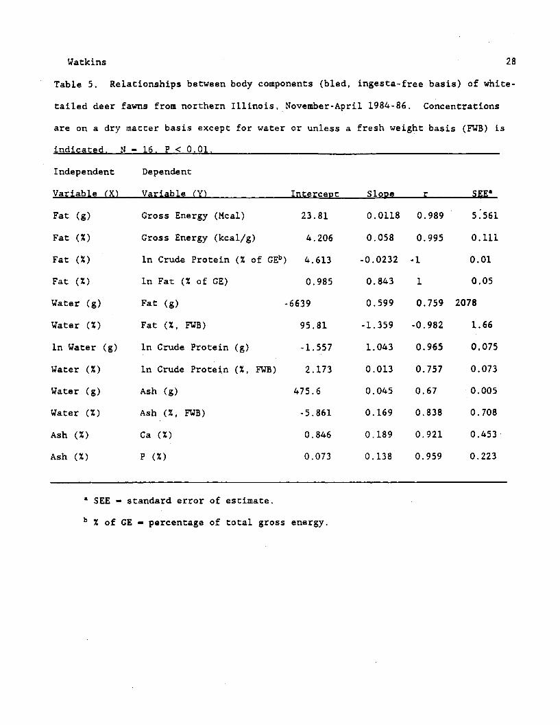
Watkins 28
Table 5. Relationships between body components (bled, ingesta-free basis) of white-
tailed deer fawns from northern Illinois, November-April 1984-86. Concentrations
are on a dry matter basis except for water or unless a fresh weight basis (FWB) is
indicated. N - 16., P < 0.01.
Independent
Variable (X)
Fat (g)
Fat (%)
Fat (%)
Fat (%)
Water (g)
Water (%)
In Water (g)
Water (%)
Water (g)
Water (%)
Ash (%)
Ash (%)
Dependent
Variable (Y)
Gross Energy (Mcal)
Gross Energy (kcal/g)
In Crude Protein (% of GEb)
In Fat (% of GE)
Fat (g)
Fat (%, FWB)
In Crude Protein (g)
In Crude Protein (%, FWB)
Ash (g)
Ash (%, FWB)
Ca (%)
P (%)
Intercept
23.81
4.206
4.613
0.985
6639
95.81
-1.557
2.173
475.6
-5.861
0.846
0.073
a SEE - standard error of estimate.
b % of GE - percentage of total gross energy.
Slope
0.0118
0.058
-0.0232
0.843
0.599
-1.359
1.043
0.013
0.045
0.169
0.189
0.138
r
0.989
0.995
-I
0.759
-0.982
0.965
0.757
0.67
0.838
0.921
0.959
SEEa
5.561
0.111
0.01
0.05
2078
1.66
0.075
0.073
0.005
0.708
0.453
0.223

Watkins
Fig. 1. The relationships between bled, ingesta-free body ether extract (BIFB EE)
(dry matter basis) and the percentages of BIFB EE contributed by the hide, viscera,
and carcass of white-tailed deer fawns during November-April from Northern Illinois,
1984-1986. Lines fitted by eye.
Fig. 2. The relationships between bled, ingesta-free body (BIFB) weight and
calculated loss of water, ether extract, crude protein, and ash per kg of BIFB
weight loss for white-tailed deer fawns during November-April from Northern
Illinois, 1984-1986.
29

Percent of BIFB EE
o oo o 8 8 8 8
+4
wm'Ii
0E
i**/
I
f- Iso
+!

Component loss(kg/kg of BIFB weight loss)
S0 0 0 0.~~~ 0 o *& » o
0m
Co
OBM
.,,.
0(a
(0
0
CA)4ý
Appendix D. Watkins, B.E., D.E. Ullrey, J.H. Witham, and J.M. Jones 1990.
Field evaluation of deuterium oxide for estimating body composition of white-
tailed deer (Odocoileus virginianus) fawns. J. Zoo and Wildl. Medicine.
21:453-456.

- . . ;. 8116
ft.~16Journal of Zoo and Wildlife Medicine 21(4): 453-456, 1990
Copyright 1990 by American Association of Zoo Veterinarians
FIELD EVALUATION OF DEUTERIUM OXIDE FORESTIMATING BODY COMPOSITION OF WHITE-TAILEDDEER (ODOCOILEUS VIRGINIANUS) FAWNS
Bruce E. Watkins, Ph.D., Duane E. Ullrey, Ph.D, James H. Witham, Ph.D.,and Jon M. Jones, M.S.
Abstract: The efficacy of using deuterium oxide dilution under field conditions to predict bodycomposition of free-ranging white-tailed deer (Odocoileus virginianus) was evaluated using 10 fawnscaptured near Chicago, Illinois, between November 1985 and March 1986. Estimated body waterwas calculated using the average blood deuterium concentration 1.5 and 2 hr after i.v. infusion.Estimated body water was correlated with true body water (r2 = 0.93) but overestimated true bodywater by 23.8 ± 1.4%. Including estimated body water in regression models significantly (P < 0.05)improved prediction of body composition versus the use of live weight alone. Estimated body water(kg) and live weight (kg) were correlated (P < 0.0001) with the ether extract (kg) (R2 = 0.93), grossenergy (Mcal) (R2 = 0.95), and crude protein (kg) (R2 = 0.93) content of the ingesta-free body.
Key words: Body composition, condition, deuterium, isotope dilution, Odocoileus virginianus,white-tailed deer.
INTRODUCTION
The condition of live free-ranging deerusually is evaluated based on body weight,external morphometry or conformation,and/or blood and serum constituents. Noneof these methods provide a quantitativemeasure of body composition. We believethat condition of deer is best expressed interms of the gross energy content (GE, Mcal)of the ingesta-free body (IFB). Isotope di-lution techniques have been used success-fully to estimate gross body composition ina variety of live animals,",4' 6'9 including cap-tive white-tailed deer (Odocoileus virgini-anus).7 Unlike tritium, deuterium is a stableisotope that can be used safely in the fieldwithout special precautions. Isotope dilu-tion using deuterium oxide (D20), there-fore, offers potential for estimating the bodycomposition of free-ranging animals.
From Durango Software, P.O. Box 2783, Durango,Colorado 81302, USA (Watkins); the Department ofAnimal Science, Michigan State University, East Lan-sing, Michigan 48824, USA (Ullrey); the Illinois Nat-ural History Survey, 607 E. Peabody, Champaign, Il-linois 61820, USA (Witham); and the IllinoisDepartment of Conservation, 524 S. Second Street,Springfield, Illinois 62706, USA (Jones).
The objective of this study was to eval-uate the efficacy of D20 dilution for pre-dicting body composition of white-taileddeer fawns under field conditions.
MATERIALS AND METHODS
Ten free-ranging white-tailed deer fawns(eight males and two females born duringMay and June) were captured by rocket netnear Chicago, Illinois, in 1985 and 1986during November (n = 2), December (n =3), January (n = 2), and March (n = 3).Capture locations and capture and handlingmethods have been described elsewhere."IAfter capture, each deer was immobilizedby an i.m. injection of 8 mg/kg ketaminehydrochloride (Vetalar, Parke-Davis, Mor-ris Plains, New Jersey 07950, USA) and 1.2mg/kg xylazine (Rompun, Haver-Lockhart,Shawnee, Kansas 66201, USA). Three fawnsrequired additional injections (approxi-mately 5 mg/kg ketamine and 1.5 mg/kgxylazine) to maintain adequate anesthesiafor 2 hr.
Each of nine fawns was injected via thejugular vein with 10 g of D20 (DLM-4 deu-terium 99.8% D, Cambridge Isotope Lab-oratories, Inc., Cambridge, Massachusetts02139, USA) that had been preweighed in
453

JOURNAL OF ZOO AND WILDLIFE MEDICINE
a 12-cc disposable syringe. One fawn wasinjected with only 5.4 g of D20 via the jug-ular vein because additional D20 was notavailable. Blood samples were obtained byjugular venipuncture from the vein oppositethe injected vein at 1.5 and 2 hr postinfu-sion. After the last blood sample was col-lected, each animal was euthanized by in-jection of T-61 euthanasia solution(National Laboratories, Somerville, NewJersey 08876, USA). Each animal was bledfrom the neck, and the weight of the bloodwas combined with the weight of the pre-vious blood samples. The contents of thestomach (rumen, reticulum, omasum, ab-omasum) and intestines (small intestine, ce-cum, large intestine, rectum) were removedand weighed. The entire carcass and viscerafrom each animal and samples of digestawere double bagged in air-tight polyethyl-ene liners and stored at - 20*C. Tissues wereground twice using a large auger grinder.Blood and tissue samples were freeze-driedand analyzed for dry matter, crude protein(CP), ether extract (EE), GE, and ash as de-scribed by Rumpler et al. 7 Blood sampleswere frozen in sealed vacuum tubes for ly-ophilization. The water fraction of the bloodsamples was analyzed for deuterium usinginfrared spectrophotometry. 2 Samples of thestomach and intestinal contents from eightdeer were analyzed for water concentration.Water contents of the ingesta of two deerwere predicted from the weights of stomachand intestinal contents using the averagewater concentrations of the eight analyzedsamples.
True body water (TBW) was calculatedby summing the water contained in the in-gesta-free body with that contained in theingesta, as determined by analysis. Esti-mated body water (EBW) was calculatedbased on the ratio between blood deuteriumconcentration and the amount of injecteddeuterium.
Linear regression analysis was performedusing the SPSS/PC+ statistical program(SPSS, Inc., 444 N. Michigan Ave., Chi-cago, Illinois 60611, USA). Forward mul-
tiple regression was used when inclusion ofmore. than one independent variable signif-icantly (P < 0.05) improved the regression.Homogeneity of regression coefficients wastested using an F-test.8 A paired t-test wasused to test for differences between 1.5- and2-hr blood deuterium concentrations.
RESULTS
Blood deuterium concentrations did notdiffer significantly between 1.5- and 2-hrpostinfusion blood samples and did not al-low dilution space to be calculated at thetime of infusion. The average of the twosamples was used to calculate EBW.
Estimated body water averaged 23.8 +1.4% (mean ± SE, n = 10) higher than TBW(Table 1). Estimated body water (% of liveweight) and TBW (% of live weight) eachwere correlated with IFB EE (%, fresh weightbasis [FFB]) and IFB GE (kcal/g, FWB) (Ta-ble 2). The slopes of the regressions did notdiffer significantly when either EBW or TBWwas used as the independent variable.
Ingesta-free body EE (kg), IFB CP (kg),and IFB GE (Mcal) were highly correlatedwith either EBW (kg) and live weight orTBW (kg) and live weight (Table 3). Pre-diction of IFB ash (kg) was not significantlyimproved by inclusion of live weight in theregression when either EBW (kg) or TBW(kg) was used as an independent variable.
DISCUSSION
Rumpler et al. 7 found that D20O equili-brated with the body water pool within 2 hrpostinfusion in adult white-tailed deer does.Based on these results, we selected samplingtimes of 1.5 and 2 hr postinfusion. The sim-ilar D20 concentrations determined in the1.5- and 2-hr samples indicate that tracerequilibration had occurred in the fawnswithin 1.5 hr.
We found EBW averaged almost 24%higher than TBW. Estimated body water al-ways exceeds TBW when a single equili-brated blood D20 concentration is used tocalculate dilution space. 6 OverestimatingTBW by more than 20% is not uncommon
454

WATKINS ET AL.-ESTIMATING BODY COMPOSITION USING D20
Table 1. Characteristics of white-tailed deer fawns collected between November and March from northernIllinois, 1985-1986.
Characteristic n x SE Range
Live weight (kg) 10 34.9 1.6 27.1-41.6IFBa weight (kg) 10 32.0 1.8 23.3-39.5True body water (kg) 8 22.2 0.8 16.7-25.5True body water (% of live weight) 8 61.1 1.6 55.9-71.2Estimated body water (kg) 10 27.4 1.1 19.5-31.4Estimated body water (% of live weight) 10 77.6 2.0 68.7-90.3Stomach contents (kg) 10 2.26 0.24 1.5-4.1Stomach water (%) 8 80.1 1.4 73.9-84.7Intestinal contents (kg) 10 0.71 0.04 0.5-1.0Intestinal water (%) 8 75.9 1.0 71.8-81:3Ingesta water (% of true body water) 8 9.4 0.7 6.5-11.8IFB ether extract (%, DMBb) 10 32.6 5.0 4.2-48.2IFB crude protein (%, DMB) 10 51.4 3.8 40.3-75.8IFB ash (%, DMB) 10 10.8 1.3 6.6-17.8IFB gross energy (Mcal/kg, DMB) 10 6.15 0.27 4.6-7.0
* Ingesta-free body.b Dry matter basis.
in single-point isotope dilution studies.9 Indomestic ruminants, single-point tracermeasurements typically result in a calculat-ed dilution space that is 10-20% greater thanTBW.' .6 It is not known why TBW is over-estimated to different degrees in differentstudies. Possible reasons include variablerates of in vivo isotope fractionation (e.g.,due to species, age, physiological status,drugs), the use of different sampling inter-vals after equilibration (i.e., the longer theinterval, the greater the overestimate), andincomplete deuterium recovery after vac-uum sublimation.4
When serial blood D20 measurements areused to extrapolate to the time of infusion,EBW is generally only 3-7% greater thanTBW in ruminants.' .6,7 In our study, thesimilarity between the 1.5- and 2-hr sam-ples made extrapolation impossible. Takingmore than two samples and extending theinterval between samples might improve theaccuracy of TBW estimates but may be im-practical for some field applications.
Even though EBW overestimated TBW,EBW, in combination with live weight, pro-vided a reasonably accurate prediction ofbody composition and significantly im-proved the prediction of body composition
over the use of live weight alone. On thisbasis, our results indicate that D20 dilutionoffers a potential nonlethal method for es-timating the body composition of deer inthe field. Additional studies will be requiredto determine EBW-body composition re-lationships for age classes other than fawns.If animals are to be released, sodium chlo-ride should be added to the D20 to make a0.85% NaCl solution (physiological saline),and sterile techniques must be used. The
Table 2. Relationships between the percentages ofestimated body water (EBW %) or true body water(TBW %) and ingesta-free body (IFB) ether extract orgross energy concentrations for white-tailed deer fawnsfrom northern Illinois. All values are on a fresh basis.n 10, P < 0.001.
Regression model r SEEb
IFB ether extract (%) =- 1.094(EBW %) + 98.310 0.87 2.91
IFB gross energy (Mcal/kg) =-0.092(EBW %) + 9.541 0.83 0.29
IFB ether extract (%) =-1.353(TBW %) + 98.328 0.97 1.53
IFB gross energy (Mcal/kg) =-0.117(TBW %) + 9.794 0.99 0.08
* Coefficient of determination.b Standard error of estimate.
455

JOURNAL OF ZOO AND WILDLIFE MEDICINE
Table 3. Linear regression models for predictingtrue body water (TBW), ingesta-free body (IFB) etherextract (EE), IFB crude protein (CP), IFB ash, and IFBgross energy (GE) from estimated body water (EBW)or TBW and live weight for white-tailed deer fawnsfrom northern Illinois. All units are in kilograms exceptGE (Mcal). n = 10, P < 0.0001 except as noted.
Regression model R2 SEEb
TBW = 0.670 (EBW) + 3.684 0.93 0.67IFB EE = 0.918 (live wt) 0.93 0.85
- 0.870 (EBW) - 4.041IFB CP = 0.075 (live wt) 0.93 0.30
+ 0.169 (EBW)- 0.997
IFB ash = 0.042 (EBW) + 0.127 0.41c 0.19'IFB GE = 9.348 (live wt) 0.95 7.93
- 7.332 (EBW)- 48.570
IFB EE = 0.907 (live wt) 0.98 0.51- 1.258 (TBW)+ 0.243
IFB CP = 0.091 (live wt) 0.92 0.33+ 0.205 (TBW)- 1.497
IFB ash = 0.060 (TBW) - 0.051 0.4 1c 0.19IFB GE = 9.381 (live wt) 0.99 3.66
- 10.937 (TBW)- 9.575
* Coefficient of multiple determination.b Standard error of estimate.P < 0.05.
combination of ketamine and xylazine usedwas usually sufficient to keep the deer an-esthetized and immobilized for over 2 hr.Captive white-tailed deer can be immobi-lized repeatedly with ketamine and xylazinewith little drug-related mortality.10 Yohim-bine could be used to hasten recovery inketamine-xylazine-immobilized animals35
after blood samples for D20 analysis havebeen collected. Ketamine, xylazine, and yo-himbine are not approved for use in food-producing animals and therefore would haverestricted use for deer populations harvest-ed for human consumption. It is not knownhow the use of other drugs (e.g., carfentanil)would influence estimates of D20 dilutionspace.
Acknowledgments: We thank W. V. Rumplerof the U.S. Department of Agriculture for thedeuterium analyses and P. A. Whetter of Mich-
igan State University for tissue analyses. Thisresearch was as substudy of the Illinois NaturalHistory Survey (INHS) Urban Deer ResearchProgram, a contribution of the Federal Aid inWildlife Restoration Project (W-87-R), the Illi-nois Department of Conservation, the U.S. Fishand Wildlife Service, and the INHS.
LITERATURE CITED
1. Arnold, R. N., E. J. Hentges, and A. H. Trenkle.1985. Evaluation of the use of deuterium oxide di-lution techniques for the determination of body com-position of beef steers. J. Anim. Sci. 60: 1188-1200.
2. Byers, F.M. 1979. Extraction and measurementof deuterium oxide at tracer levels in biological fluids.Anal. Biochem. 98: 208-213.
3. Jessup, D. A., W. E. Clark, P. A. Gullett, and K.R. Jones. 1983. Immobilization of mule deer withketamine and xylazine, and reversal of immobilizationwith yohimbine. J. Am. Vet. Med. Assoc. 183: 1339-1340.
4. Johnson, R. J., and D. J. Farrell. 1988. Theprediction of body composition in poultry by esti-mation in vivo of total body water with tritiated waterand deuterium oxide. Br. J. Nutr. 59: 109-124.
5. Mech, L. D., G. D. Del Giudice, P. D. Karns,and U. S. Seal. 1985. Yohimbine hydrochloride asan antagonist to xylazine hydrochloride-ketamine hy-drochloride immobilization of white-tailed deer. J.Wildl. Dis. 21: 405-410.
6. Robelin, J. 1984. Prediction of body compo-sition in vivo by dilution technique. In: Lister, D. (ed.).In Vivo Measurement of Body Composition in MeatAnimals. Elsevier, London. Pp. 106-112.
7. Rumpler, W. V., M. E. Allen, D. E. Ullrey, R. D.Earle, S. M. Schmitt, and T. M. Cooley. 1987. Bodycomposition of white-tailed deer estimated by deute-rium oxide dilution. Can. J. Zool. 65: 204-208.
8. Snedecor, G. W., and W. G. Cochran. 1967.Statistical Methods, 6th ed. Iowa State Univ. Press,Ames, Iowa.
9. Shields, R. G., Jr., D. C. Mahan, and F. M. Byers.1983. Efficacy of deuterium oxide to estimate bodycomposition of growing swine. J. Anim. Sci. 57: 66-73.
10. Watkins, B. E., D. E. Ullrey, R. F. Nachreiner,and S. M. Schmitt. 1983. Effects of supplementaliodine and season on thyroid activity of white-taileddeer. J. Wildl. Manage. 47: 45-58.
11. Witham, J. H., and J. M. Jones. 1987. Deer-human interactions and research in the Chicago met-ropolitan area. In: Adams, L. W., and D. L. Leedy(eds.). Integrating Man and Nature in the MetropolitanEnvironment. Proc. Natl. Symp. Urban Wildl., Natl.Inst. Urban Wildl., Columbia, Maryland. Pp. 155-159.
Received for publication 7 May 1990.
456

Appendix E. Cisneros, J.G. 1987. Helminthic and protozoan parasites of white-
tailed deer in urban areas of northeastern Illinois. Unpub. rep. sub. to Ill.
Natural History Survey-Wildl. Sec., Champaign. 15pp.

Illinois Natural History SurveyWildlife Section
Urban Deer Study
Helminthic and Protozoan Parasitesof White-tailed Deer
in Urban Areas of Northeastern Illinois
Final Report
Jose G. Cisneros, Investigator
January, 1987
Submitted to:I.N.H.S. Wildlife SectionNatural Resources Building, Room 279607 E. Peabody DriveChampaign, IL 61820

Helminthic and Protozoan Parasites of White-tailed Deerin Urban Areas of Northeastern Illinois
Jose G. Cisneros
This report is part of the Urban Deer Study of the Illinois Natural History Survey. The project was a
determination of the helminthic and protozoan parasites of white-tailed deer (Odocoileus virginianus) through fecal
analysis. Animals sampled in this study are part of white-tailed deer herds found in urban locations of northeastern
Illinois. Within the text is included detailed methodology, results of examinations, discussion of the significance of these
results, and problems perceived in this study with recommendations for improvements.
METHODS
Over one thousand fecal samples were collected by Dr. James Witham during post mortem examinations of road-
killed white-tailed deer during a twenty-three month period (December 1983 to October 22, 1985). Samples were frozen
and stored for a period of one to three years. For parasitological examination, 270 samples were chosen from four sites:
Northwest Cook County, Des Plaines, Busse Woods, and Non-Cook County. Within each location, samples were divided
according to season collected - summer, fall, winter, and spring. All samples were from deer over one year of age.
Samples of feces were thawed for one hour before use and were processed for fecal flotation after Samuel and
Trainer (1969). One gram of feces was placed into a beaker with 10ml of water. The pellets were broken up completely
and the mixture was poured through standard cheesecloth into another beaker. Fecal material in the cloth was pressed with
a lab spatula to remove all liquid. The liquid was then poured into a 15ml centrifuge tube and spun at 2200rpm for ten
minutes in a clinical centrifuge. The supernatent was discarded and 6ml of Sheather's sugar solution (Levine et al., 1960)
was added to the sediment and mixed with a spatula. Sugar solution was added to fill the tube, and the mixture was
centrifuged for two minutes at 1100 rpm. After centrifugation, a positive meniscus was created on the tube by adding fresh
sugar solution, and a 22mm square coverglass was placed over the top of the tube. After several minutes, the coverglass
was removed and transferred to a glass slide. The entire surface of the coverglass was systematically examined for helminth
eggs, larvae and coccidial oocysts with the aid of a compound microscope. Data for each sample were recorded on a
standardized data sheet Size was determined with an ocular micrometer. Relevant taxonomic keys and literature utilized in

2
identifying parasites included Kates and Shorb (1943), Becklund (1964), Samuel and Beaudoin (1965), Levine (1968) and
Anderson and Samuel (1969).
RESULTS
Two hundred seventy fecal samples from four different areas in northeastern Illinois were examined. Examination
revealed five species of nematodes and two species of coccidia. Seventy-four animals (28%) were found to carry one of
more parasites which were represented by eggs, first stage larvae and oocysts (Table 1). Anatomical location of parasite in
the host, number of deer infected, prevalence, intensity and size range is given for all parasites. Study wide, the
trichostrongyloids showed the highest prevalence (11.5%) of all parasites found. ( The designation "trichostrongyloids"
in the tables includes eggs of the genera Haemonchus. Ostertagia, and Trichostrongylus, and is used due to the difficulties
involved in distinguishing the eggs of these three genera. The genera are closely related and species identification based on
eggs alone is not feasible. Eggs seen in this study could belong to one or more of the three genera.)
TABLE 1
Parasite prevalence and intensity of Illinois urban white-tailed deer as determined by fecal flotation.
Parasite # Infected Prevalence Intensity Size (4 )#examined ( % ) Range Mean
Trichostrongyloids 31/270 11.5 1-29 2.5 60-89x30-50
Oesophagostomum venulosum 5/270 2 1-4 2 70-100x36-55
Nematodirus odocoilei 6/270 2 1-9 3 140-190x53-80
Capillaria bovis 8/270 3 1-3 1.5 40-55x21-32
ParelaphostrongYlus tenuis 16/270 6 1-14 3.5 190-350x10-17
Eimeria mecordocki 19/270 7 1-25 3 25-47x15-30
Eimeria madisonensis 3/270 1 1-2 1.5 17-22x17
Overall infection rate for study: 28%

Data for individual locations was separated to characterize the infections present in each. Light infections of three
nematode species and one Eimeria species were found in Northwest Cook County (Table 2). Prevalence for Northwest
Cook County is 25%.
Three nematode species and two species of coccidia were found in the Des Plaines area deer (Table 3). The
Eimeria mccordocki infection rate is the highest for any area. Overall prevalence for the Des Plaines area is 24%.
Four species of nematodes and two species of Eimeria were discovered in Busse Woods samples (Table 4). The
largest overall infection rates of this study were from the trichostrongyloid eggs (16%) and the E. tenuis larvae (14%)
found in the Busse Woods samples. Prevalence for the Busse Woods collection is 41%.
Only three species of nematodes were found in the Non-Cook County samples, and low prevalences were
determined for each (Table 5). The overall prevalence for Non-Cook samples is 11%.
Individual parasite prevalences for all four areas are compared in Table 6.
TABLE 2
Parasite prevalence and intensity for Northwest Cook County white-tailed deer.
Parasite Prevalence ( %) IntensityRange Mean
Trichostrongyloids 8 1-2 1
Oesophagostomum venulosum 0 - --
Nematodirus docoilei 6 1-9 4.5
Capillaria bois 2 1 1 1
Parelaphostrongylus 0 - -
Eimeria m ordocki 10 S 1-5 2
Eimixia madisonensis 0
Animal sample size: 52Animals found infected: 13
Infection rate: 25%

TABLE 3
Parasite prevalence and intensity for Des Plaines white-tailed deer.
Parasite Prevalence ( % ) IntensityRange Mean
Trichostrongyloids 10 1-4 2.5
Oesophagostomum venulosum 0
Nematodirus odooilei 2 1 1
Capillaria, b.i 0 - --
Parelaphostrongylus mtenui 2 1 1
Eimeriamccordocki 12 1 1-25 6
Eimi madisonensis 3.5 X- 1-2 1.5
Animal sample size: 58 Infection rate: 24%Animals found infected: 14
TABLE 4
Parasite prevalence and intensity for Busse Woods white-tailed deer.
Parasite Prevalence ( % ) IntensityRange Mean
Trichostrongyloids 16 i j 1-29 3
Oesophagostomum venulosum 5 5 1-4 2
Nematodirus odocilei 0 - --
Caillaria bovis 5 1-3 1.5
ParelaphostrongXlus tenuis 14 ,5 1-14 4
Eimria mcordocki 6 1-2 1
Eimeria madisonensis 1 1 1
Animal sample size: 105Animals found infected: 43
Infection rate: 41%

TABLE 5
Parasite prevalence and intensity for Non-Cook County white-tailed deer.
Parasite Prevalence ( % ) IntensityRange Mean
Trichostrongyloids 7 1 1
Oesophagostomum venulosum 0 C - --
Nematodirs odgoile 4 1 1-3 2
Capillaria bovis 4 2 2
Parelaphostrongylus enuis 0 C
immeiam rdocki 0
Eim.i madisonensis 0 -
Animal sample size: 55Animals found infected: 6
Infection rate: 11%
TABLE 6
Comparison of parasite prevalences in white-tailed deer from Northwest Cook County, Des Plaines,Busse Woods and Non-Cook County areas.
PARASITE
Nematoda:
Trichostrongyloids
Oesophagostomum venulosum
Nematodirus odocoilei
Capillaria bovis
Parelaphostrongylus te uis
Protozoa:
Eimeria mccordocki
PREVALENCE
NW Cook Des Plalnes Busse Woods
10
0
2
0
2
1210
16
5
0
5
14
6
0 3.5 1
Non-Cook
Eimeria madisonensis

6
Parasite intensities were generally low. Most eggs, larvae, and oocysts were present in numbers less than 10.
The largest intensities seemed to correspond to the areas and particular parasite species with the highest prevalences: Des
Plaines, ,. mccordocki: Busse Woods, trichostrongyloids and ,. tenuis.
Seasonal differences in parasite prevalence and intensity were examined between all sites and within each site.
Winter samples showed the greatest percentage of infections (31%), but the infection rates of summer, spring and fall were
only slightly lower (26%, 27% and 25%, respectively). Intensities were uniformly low except for relatively high Eimria
oocysts numbers in spring and fall and trichostrongyloid eggs and E. tenis larvae in isolated animals during the summer.
Parasite assemblages also changed with seasons. The greatest number of multiple parasite infections within
single deer occurred in the summer and winter seasons. Trichostrongyloid eggs were found most often in spring and
summer, and Capillaria bovis eggs were found in the greatest number of animals in the fall. Oocysts of the coccidia
iimeria were found most often in winter samples. Parelaphostrongylus Sis larvae were found in fecal samples collected
at all times of the year (Table 7).
TABLE 7
Seasonal parasite prevalence (%) for Illinois urban White-tailed deer.
S,3 PREVALENC-.7
PARASITE Summer Fall Winter SpringNematoda:
Trichostrongyloids 19 1 3 2. 7 4 16 2-
Qesophagostomum venulosum 0 0 3 2- 3 2-
Nematodirus odocoilei 5 3 5 4,4 0 0
Capillariabovis 0 8 ( 3 2 1 I
Parelaphostrongylus t~nis 5 3 6 5 7 1 5 q
Protozoa:
Eimeria spp. 8 3 16 1 4 3
Within locations, Northwest Cook County and Non-Cook County showed the fewest infections during all
seasons with relatively little winter and spring parasite activity (Tables 8 and 11). Des Plaines and especially Busse

Woods exhibited parasite infections year-round (Tables 9 and 10). Winter and spring infections at the latter two sites are
most conspicuous by their numbers when compared to the Northwest Cook and Non-Cook samples.
TABLE 8
Seasonal parasite prevalence (%) for Northwest Cook County white-tailed deer.
PREVALENCE
PARASITE Summer Fall Winter Spring
..- --------------------------------. , ..... .......------------
Trichostrongyloids 20 3 I1 0 0
Qesophagostomumn veulosum 0 0 0 0
Nematodirus odoilei 13 2- 7 I 0 0
Capillariaboris 0 7 I 0 0
Parelaphostrongylus t~sgis 0 0 0 0
Protozoa:
-imeria spp. 13 A- 0 43 3 0
TABLE 9
Seasonal parasite prevalence (%) for Des Plaines white-tailed deer.
PREVALENCE
PARASITE Summer Fall Winter Spring
Trichostrongyloids 8 1 0 13 20 3
Oesophagostomum venulosum 0 0 0 0
Nematodirus odocoilei 0 7 I 0 0
Capillaria bovis 0 0 0 0
Parelaphostrongylus tenuis 0 7 I 0 0
Protozoa:
Eimeria snp. 8 I 13 o 20 1 13 ". ...• g K

8
TABLE 10
Seasonal parasite prevalence (%) for Busse Woods white-tailed deer.
PREVALENCE
PARASITE Summer Fall Winter Spring
Nematoda:
Trichostrongyloids 29 , 11 11 23 7
Oesophagostomum venulosum 0 0 6 2- 7 2
Nematodirus odocoilei 0 0 0 0
Capillariab 0 11 > 6 > 3 1
Parelaphostrongvlus tenuis 14 3 17 3 14 5 13 N
Protozoa:
Eimeia spp. 10 -- 0 14 5 3 I
TABLE 11
Seasonal parasite prevalence (%) for Non-Cook County white-tailed deer.
PREVALENCE
PARASITE Summer Fall Winter Spring
Nematoda:
Trichostrongyloids 14 0 0 14 .
Oesophagostomum venulosum 7 1 0 0 0
Nematodirus odocoilei 7 6 1 0 0
Capillariabovis 0 12.5 . 0 0
Parelaphostrongvlus tenui$ 0 0 0 0
Protozoa:
Eim~ti& ~PP* 0 0 0Eieria spp.

9
DISCUSSION
A single published report exists concerning abomasal and intestinal helminths of white-tailed deer in Illinois
(Cook et al., 1979), and no published reports are available with respect to protozoa infections. The study by Cook et al.
involved the necropsy of eighty-four deer and compared parasite infections in deer from northern and southern regions of the
state. Cook's necropsies revealed the nematodes Gongylonema pulchrum. Apteraia odocoilei, Haemonchus contortus,
Nematodirus sp., Trichur sp., and Setaria Xhi, and the cestode Mnizia benedeni in the northern sample (Carroll and Jo
Daviess counties). Never published separately, Schaeffler and Levine (1968) reported data indicating an approximate 50%
infection rate for E. tenuis in Illinois deer. The present study found two species of nematodes not previously reported for
northern Illinois deer- Oesophaostomum venulosum and Capillaria bvis.
This study is the first report of protozoans in Illinois deer. Two species of coccidia - Eimeria mccordocki and
Eia madisonensis, were found in the samples studied,
Although not previously reported in northern Illinois, Q. venulosum, C. oFis, E. mccordocki and E.
madisonensis, as well as the other parasite species found in this study, are all well known and common parasites of white-
tailed deer in the United States. Davidson et al. (1981), the most recent compendium of disease and parasites of white-
tails, lists prevalences of all these parasites in the various states where studies have been made. Particular studies which
found similar assemblages include: Anderson and Samuel (1969) (samples from Pennsylvania, Texas and Wisconsin);
Beaudoin, et al (1970) (samples from Pennsylvania); Samuel and Beaudoin (1965; 1966) (samples from Pennsylvania);
Samuel and Trainer (1969) (samples from Wisconsin); and Prestwood et al (1973) (samples from southeastern United
States, Texas and the Virgin Islands) and Cisneros (in prep.) (samples from Missouri). In most of the other studies,
parasite prevalence was greater than that discovered in Illinois. Several explanations are possible. The most readily
apparent is that Illinois deer are not as heavily parasitized as deer in other areas. Data from the northern study site of Cook
et al. (1979), however, shows a significantly higher set of prevalence values with infection rates more similar to those
found in other states than to those in the current study. This first explanation, therefore, is probably not valid.
A second possible reason for low parasite prevalence is the basic weakness of the fecal flotation procedure in
indicating the full extent of an infection. Samuel and Trainer (1969) used fecal flotation to check Wisconsin deer for
internal parasites and did identify eggs, larvae, and oocysts of many of the same species found in the present study.
10
However, their flotation findings were supplemented by necropsy recovery of parasites from deer in the study area. In
most cases, necropsies revealed two to three times as many helminth infections as revealed by fecal flotation. In some
cases, parasites not found in the flotation work were discovered during necropsy. Although the flotation method is the
easiest and fastest way to assess the parasite assemblage within deer, necropsy of fresh kills is still the procedure of
choice in order to receive the most accurate estimates of parasite prevalence and intensity. Most of the deer parasite
studies previously cited were done by direct necropsy examination.
Finally, low prevalence and intensity figures of this study could have been influenced by prolonged freezing of
the samples. The freezing and thawing processes can be very destructive to eggs and oocysts, and in fact, many
trichostrongyloid eggs identified in this study were ruptured. Rupture most likely occurred as a result of a period of
dessication prior to collection and post-collection freezing and thawing cycles before finally being examined. Ruptured
eggs are often not recognizable as eggs and consequently are not counted. In fresh fecal samples, the presence of ten to
twenty eggs normally does not indicate a heavy infection. However, due to potential loss of eggs, larvae and oocysts
through the freezing process used in this study, infections represented by ten or more eggs, larvae or oocysts may actually
indicate a heavy infection with lighter infections represented by only one or two eggs or oocysts. Those infections that
are found may be perceived as lighter infections than they truly were, and some lighter or less resistant infections might be
totally missed.
The last two factors described above may have contributed significantly to an apparent low parasite prevalence
relative to the actual number of infected deer that may exist in the field.
Seasonal variation in parasite prevalence has been noted both between and within study sites. The comparison of
overall seasonal prevalences: winter (31%), spring (27%), summer (26%) and fall (25%), indicates that the differences in
overall infection rates are not statistically significant. The changing composition of parasite assemblages and the
corresponding change in infection rates are noteworthy. Overall, trichostrongyloid prevalence is high in the spring and
summer compared to fall and winter months (16%, 19% and 3%, 7% respectively). Eggs of the trichostrongyloid
complex require warm temperatures and adequate moisture to develop - conditions most likely to occur during spring and
summer. These nematodes continue to produce eggs during fall and winter, but in smaller numbers than when external
conditions are favorable. The need for warm, moist conditions is reflected in the trichostrongyloid seasonal prevalence
differences. During the winter, the prevalence of Eim.ria spp. oocysts is also relatively high. Coccidia oocysts also

11
require heat and moisture to develop outside the deer, but oocysts are none-the -less released fairly continuously in the
feces throughout the year. Eimeria spp. oocysts are very resistant to environmental extremes. The summer infection rate
of 8% indicates a strong Eimeria presence. The winter rate of 16% shows an even greater presence which is probably
related to changing habits of deer in this study. Deer typically have less food and more contact with other deer during
winter due to the limited food resources. In the northern states, the deer habit of "yarding up" during the winter can lead to
greatly increased contact between deer. Poor nutrition results in a reduced resistance to internal parasites. Coccidia
multiply within an animal, and the parasite is spread to other deer feeding in the same area as the infected animal.
The expanded parasite assemblages found in the summer are attributable to the ideal summer growth situations for
many parasite species. During winter months, the increased chance of cross transmission and the relatively debilitated
state of health of deer result in expanded parasite assemblages.
In terms of each location, Eimkia spp. winter infection rate in Northwest Cook is high (43%) in spite of a
small sample size. However, the samples did not indicate a high parasite intensity. The high infection rate may be due to
the poor nutritional and overcrowded situation described above. The remainder of the protozoan infection record for
Northwest Cook is unremarkable.
Busse Woods shows a year-round parasite presence of all but one of seven parasite species found, indicating a
healthy parasite population supported by the conditions of the deer host environment.
Des Plaines and Non-Cook county areas are unremarkable in their seasonal parasite prevalences.
Based on the findings of this study, Northwest Cook county and Non-Cook county areas have the smallest
parasite assemblages and the lowest parasite prevalences within their populations. Des Plaines and Busse Woods have
significantly larger assemblages and prevalences. Northwest Cook and Non-Cook deer populations are described as low
density and high quality with a high nutritional plane. These descriptions are in line with the results of this
parasitological study. Low density and good nutrition lead to healthy deer which encounter each other only rarely. These
factors are all barriers against parasite transmission and large parasite intensities. High density and poor population quality
lead to populations more susceptible to cross-transmission and harboring larger numbers of parasites. Such a situation is
seen in Des Plaines and Busse Woods deer.

12
PARASITE LIFE CYCLES AND ASSOCIATED PATHOGENICITY
Knowledge of each specific parasite's life-cycle will help to explain the influence of seasons and herd density on
the occurrences of the parasite.
Ostertaga daocQilei, Q. mossi, Haemonchus ontoiS, and Nematodirus odocoilei are all trichostrongyloids of
the abomasum and share a common life cycle. Eggs are deposited in the feces and given the neccessary conditions (i.e.
oxygen, moisture and warm temperatures), the eggs hatch within one to two days and the first stage larvae emerge. Still
within the feces, the rhabiditiform larvae undergo two molts within the span of a few days. The infective third stage larvae
then climbs onto browse where it is ingested by feeding deer. Larvae grow to adults within the gastrointestinal tract
Pathology associated with trichostrongyloids is blood loss leading to weakness, emaciation and anemia
(Davidson et al., 1981; Olsen, 1962). Van Volkenberg and Nicholson (1943) found that deer without adequate browse and
under seasonally poor nutritional conditions were susceptible to starvation often accompanied by heavy parasitism,
especially by trichostrongyles. Although trichostrongyles contributed to the deaths of a few deer in their study, they
claimed that parasite infections were apparently unimportant among deer on ranges with sufficient food.
Q. odocoile. Q. mossi and N. odocoilei are all species specific to white-tailed deer. There have been no reports
of these parasites in domestic ruminants. There is no threat to humans from any of the parasites due to the very specific
biology and ecology of these parasites which restricts them to inhabiting white-tailed deer.
Haemonchus contortus has been reported in cattle (os ta S) and sheep (Ovis ar) as well as deer. Some
evidence points to the feasibility of cross-transmission between these three hosts. Successful laboratory infections have
been produced with sheep being infected with deer H. ontortus and vice versa (Samuel, 1968). Prestwood and Pursglove
(in Davidson et al., 1981) indicate that although cross-infection has been proven possible in the laboratory and sheep,
cattle and deer do all carry H. contortus. much data is still needed to determine whether the parasite infections are exchanged
in nature and whether they are a pathogenic threat in all species concerned.
Capillaria bois a parasite of the small intestine, is part of the Trichurata and little is known about its life cycle.
This species is widely distributed throughout the U. S. and infects cattle as well as deer. Its pathogenicity is unknown.
Low infection intensities and low prevalences found in this and other studies (Samuel and Trainer, 1969) would seem to

13
indicate that this species is unimportantant pathologically to white-tailed deer. Low prevalences in deer would indicate a
poor potential as parasite reservoirs for domestic ruminants such as cattle. There is no threat to humans from this parasite.
Oesophagostomum venulosum is a strongyle parasite of the colon. Infective third stage larvae develop on the
ground five to six days after exposure to optimum conditions of temperature and moisture (Levine, 1968). After
ingestion, larvae enter the wall of the intestine and molt to the fourth stage. Seventeen to twenty-two days after infection,
these larvae molt to the adult stage. No pathogenic effects have been reported for white-tailed de. Q. venulosum has
been reported from a number of wild and domestic ruminants worldwide. In the U.S. this parasite has been reported in
cattle, sheep, and goats (Canr hiraU) (Shorb, 1939; Whitlock, 1939; Levine, 1963) where it can damage the intestinal
wall. The low parasite prevalence and intensity found in this study and in others probably makes white-tailed deer
populations poor infection reservoirs from which to infect other ruminants. There is no threat to humans from this
parasite.
Parelaphostronglus tenni , the meningeal worm which inhabits the brain and spinal cord, has been of some
importance in the last twenty years due mostly to its destructive effect on non-natural hosts, in particular moose (Al1a
alg)., reindeer (Ranifr aandus) and elk (CrMS canadensis) (Anderson, 1965; 1970; Carpenter et aL, 1973; Karns,
1967; Prestwood and Smith, 1969). E. tenuis infections are acquired by ingestion of gastropod intermediate hosts
containing infective third stage larvae. Eggs develop in the heart and lungs into first stage larvae which are swallowed and
passed in feces. First stage larvae penetrate the foot of terrestrial snails where they grow and undergo two molts. The
infective third stage larvae is acquired by deer when infected snails are accidentally ingested with browse. Third stage
larvae migrate into the nervous system and develop into adult forms finally migrating into the cranium. As a natural host,
the pathogenic effect of . u on the white-tailed deer appears minimal. The prevalence of this parasite can be
anywhere between 5% and 86% nationwide. In experimental conditions, heavy infections are accompanied by depression,
weakness, ataxia, and posterior paralysis (Davidson et al., 1981). Massive infections, with visible signs, are considered
extremely rare under field conditions. E. tenuis infections have been found naturally and have been experimentally
established in sheep,and goats (Anderson and Strelive, 1972; Nielson and Aftosmis, 1964). The real threat of this parasite
is to other native American ungulates including moose, elk, and caribou and exotics such as fallow deer (Dama dama).
Severe neurologic disorder resulting from P. tenuis infiltration of the brain has been documented in all these species.
There is no threat to humans from this parasite.

14
Protozoan infections by Eimma mccordocki and E. madisonensis are acquired by ingestion of sporulated oocysts.
Unsporulated oocysts are passed in feces and exposure to oxygen and moisture outside the host leads to sporulation. Heavy
infections are marked by diarrhea, sometimes leading to emaciation, apathy, passage of blood and ultimately death
(Davidson, et al., 1981). Evidence suggests infection intensity declines with the deer's age due to acquired resistance
resulting from previous infections. As previously discussed, crowded conditions and poor nutrition contribute to Eimeria
infections. Anderson and Samuel (1969) report that both E. mccordocki and E. madisonensis are found only in white-tailed
deer. These parasite are therefore very species specific and there is little chance of transmission to domestic ruminants and
no threat to humans.
SUMMARY AND CONCLUSIONS
The low prevalences and low intensities indicate that none of the deer in this study were heavily parasitized, nor
do they show a threat to the general deer population in terms of parasitic infection. In the most general terms, the results
of this study can be seen as an indicator that deer of the four study areas, Northwest Cook County, Des Plaines, Busse
Woods, and Non-Cook County, are relatively healthy. The deer of Des Plaines and Busse Woods may not be as healthy as
those of Northwest Cook and Non-Cook, but this phenomenon may be attributable to the differences in density and
nutritional quality of their respective areas. Studies such as those by the Southeast Cooperative Wildlife Disease Study
(Eve and Kellogg, 1977) and Demarais, et al. (1983) are attempting to construct deer herd health indices which utilize
intensity of parasite infections to show a positive correlation to deer density. The aim is to create an index of correlations
so that by checking a relatively small sample of the herd on a regular basis and comparing the parasite count to the
established index it is possible to determine the density and health of the herd. This study in no way approaches that level
of sophistication, but it does serve to inform the investigator of parasites present in the deer and lend support to any
previously suspected trends in the population.
15
FINAL COMMENTS ON THE EFFECTIVENESS OF THIS STUDY
All samples were processed as one gram of feces so that intensity is measured as number of parasite eggs per one
gram of feces. The term "intensity" is relatively useless in terms of parasite eggs and fecal flotations as a whole since
adult parasites are capable of producing many eggs. Eggs counted from one animal for a single species of parasite may
have been created by one or by a dozen nematodes. There are no rules concerning numbers of males and females; only
dissection and extraction can determine exact parasite population numbers. Fecal flotio is useful as a tool to establish
parasite assemblages, but not intensities. The exception is when the number of eggs, larvae or oocysts is so large that a
heavy infection can be deduced. Such was not the case in this study. There were no indications of heavy or massive
infections in any of the samples examined. Samples which did contain parasites contained too few specimens to allow
estimation of the number of adult parasites involved.
Mare infections might have been detected and the accuracy of this study incraed if the samples had been stored
in 10% formalin rather than fron for one to three yeas. Experience shows the condition of parase eggs and oocysts is
significantly better after storage in formalin than after freezing.
ACKNOWLEDGEMENTS:
I would like to thank Dr. J. Witham for the opportuty to work on this Urban Der Study project. I am also
very grateful to Dr. Glen Sanderson, Dr. Sue Wood and Dr. Anderson for their help in providing laboratory space and
equipment. Finally, I would like to thank my wife, Lee Anne, for her patience and valuable typing skills, and Dr. Leslie
Uhazy for reviewing the manuscript

Literature Cited
Anderson, R. C. 1965. An examination of wild moose exhibiting neurologic signs in Ontario. Can. J. Zool. 43: 635-639.
Anderson, R. C. 1970. Neurologic disease in reindeer (Rangifer tarandu taanus) introduced into Ontario. Can. J. Zool.49: 159-166.
Anderson, D. R. and W. M. Samuel. 1969. Eimeria (Protozoa: Eimeridae) from white-tailed deer (Odocoileus virginianus)in Pennsylvania, Texas, and Wisconsin, with descriptions of two new species. Bull. Wildlife Dis. Assoc. 5: 351-356.
Anderson, R. C. and U. R. Strelive. 1972. Experimental cerebrospinal nematodiasis in kids. J. Parasitol. 58: 816.
Becklund, W. W. 1964. Revised checklist of internal and external parasites of domestic animals in the U. S. andpossessions and Canada. Am. J. Vet. Res. 25: 1380-1416.
Carpenter. J. W., H. E. Jordon, and B. C. Ward. 1973. Neurologic diseas in wapiti naturally infected with meningealworms. J. Wildlife Dis. 9: 148-155.
Cook, T. W., B. T. Ridgeway, R. Andrews, J. Hodge. 1979. Gastrointestinal helminths in white-tailed deer (Odocoileusvirginianus) of Illinois. J. Wildlife Dis. 15: 405-407.
Davidson, W. R. , F. A. Hayes, V. F. Nettles, F. E. Kellogg, eds. 1981. Diseases and parasites of white-tailed deer. TallTimbers, Tallahassee, Fl., 458 pp.
Demarais, S., H. A. Jacobson, and D. C. Guynn. 1983. Abomasal parasites as a health index for white-tailed deer inMississippi J. Wildlife Mgmt. 47: 247-252.
Eve, J. H. and F. E. Kellogg. 1977. Management implications of abomasal parasites in southern white-tailed deer. J.Wildlife Mgmt. 41; 169-177.
Karns, P. D. 1967. Pneumostrongylus tenuis in deer in Minnesota and implications for moose. J. Wildlife Mgmt. 31:299-303.
Levine, N. D. 1963. Weather, climate and the bionomics of ruminant nematode larvae. Adv. in Vet Sci. 8: 215-261.
Levine, N. D. 1968. Nematode parasites of domestic animals and of man. Burgess, Minneapolis, Mn. 600 pp.
Levine, N. D., K. N. Mehra, D. T. Clark, and I. J. Aves. 1960. A comparison of nematode egg counting techniques forcattle and sheep feces. Am. J. Vet. Res. 21: 511-515.
Kates, K. C. and D. A. Shorb. 1943. Identification of eggs of nematodes parasitic on domestic sheep. Am. J. Vet. Res. 4:54-60.
Nielson, S. W. and J. Aftosmis. 1964. Spinal nematodiasis in two sheep. J. Am. Vet. Med. Assoc. 144: 155-158.
Olsen, 0. W. 1962. Animal parasites: their biology and life cycles. Burgess, Minneapolis, Mn. 346 pp.
Prestwood, A. K. and S. R. Pursglove. 1975. Helminth parasitisms among intermingling insular populations of white-tailed deer, feral cattle, and feral swine. J. Am. Vet. Med. Assoc. 166: 787-789.
Prestwood, A. K. and J. F. Smith. 1969. Distribution of meningeal worm (Pneumostrongylus tenuis~) in deer in thesoutheastern United States. J. Parasitol. 55: 720-725.
Prestwood. A. K., F. A. Hayes, J. H. Eve, and J. F. Smith. 1973. Abomasal helminths of white-tailed deer insoutheastern United States, Texas and the Virgin Islands. J. Am. Vet Med. Assoc. 163: 556-561.

Samuel, W. M. 1968. Endoparasites of domestic ruminants and white-tailed deer. Tr. North Am. Wildlife Conf. 33: 364-372.
Samuel, W. M. and R. L. Beaudoin. 1965. Identification of eggs and larvae of nematodes parasitic in deer in Pennsylvania.Proc. Penn. Acad. ScL 39: 73-77.
Samuel, W. M. and R. L. Beaudoin. 1966. Evaluation of two survey methods for detection of helminth infections inwhite-tailed deer (Qdocoileus virginianus). Bull. Wildlife Dis. Assoc. 2: 100-107.
Samuel, W. M. and D. 0. Trainer. 1969. A technique for survey of some helminth and protozoan infections of white-taileddeer. J. Wildlife MgmL 33: 888-894.
Schaeffler, W. and N. Levine (unpub. data, p. 287). 1968. In: Nematode parasites of domestic animals and of man. Editedby N. D. Levine. Burgess, Minneapolis, MN. 600 pp.
Shorb, D. A. 1939. Differentation of eggs of various genera of nematodes parasitic in domestic ruminants in the U. S. U.S. Dept of Agr. Tech. Bull. 694: 1-10.
Van Volkenburg, H. L. and A. J. Nicholson. 1943. Parasitism and malnutrition of deer in Texas. J. Wildlife MgmL 7:220-223.
Whitlock, S. C. 1939. The prevalence of disease and parasites of white-tailed deer. Tr. 4th North Am. Wildlife Conf. pp.244-249.

Appendix 1Infection Data by Specimen
Northwest Cook County
T = TrichostrongyloidN = Nematodirus0 = OespohagostomumC = CapillariaP = ParelaphostrongylusE = Eimeria
UDS # Season Confirmed General Infection InformationLIUCC',u'J
E (micropyle) 28-30 x 15-20,% 5 foundE (micropyle) 35 x 25 , 1 found
Coccidia egg, 35 x 15.,, 1 found
N egg, 155-170 x 75.- 9 foundDark bioperculate eggs, 40 x 2 5A, 1 found(possible C)
T egg (ruptured) 80 x 45A, 1 found
Large, dark coccidian (micropyle present) 50 x 30 m, 1 found (sheep?); T egg, 75 x 50., 1 found; Negg, 165 x 75.A, 1 found
E 38 x 25 , 1 found; egg-like structure, 35 x 20 m, 6 -8 found; N egg (deflated) 160 x 754, 2found; N egg (whole), 155 x 80q, 1 found
T egg (deflated), 80 x 45-50U, 2 found
T egg, 70 x 404, 1 found
Data #
1234567891011121314
1516171819202122232425
262728
293031323334353637
44510435971520991473912537998963979983
454474855428417439003006329866846
256252844
814842813856165109157812816
wwwwwwFFFWFFFF
FFSFFFFFFSS
SSS
SSSSSpSpSpSS
xx
x
xx
x
x
x
x
x
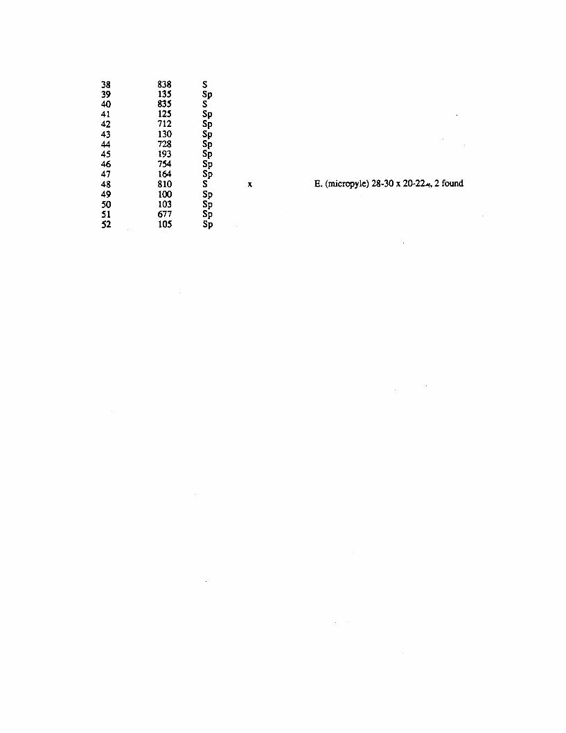
38 838 S39 135 Sp40 835 S41 125 Sp42 712 Sp43 130 Sp44 728 Sp45 193 Sp46 754 Sp47 164 Sp48 810 S x E. (micropyle) 28-30 x 20-22.q, 2 found49 100 Sp50 103 Sp51 677 Sp52 105 Sp
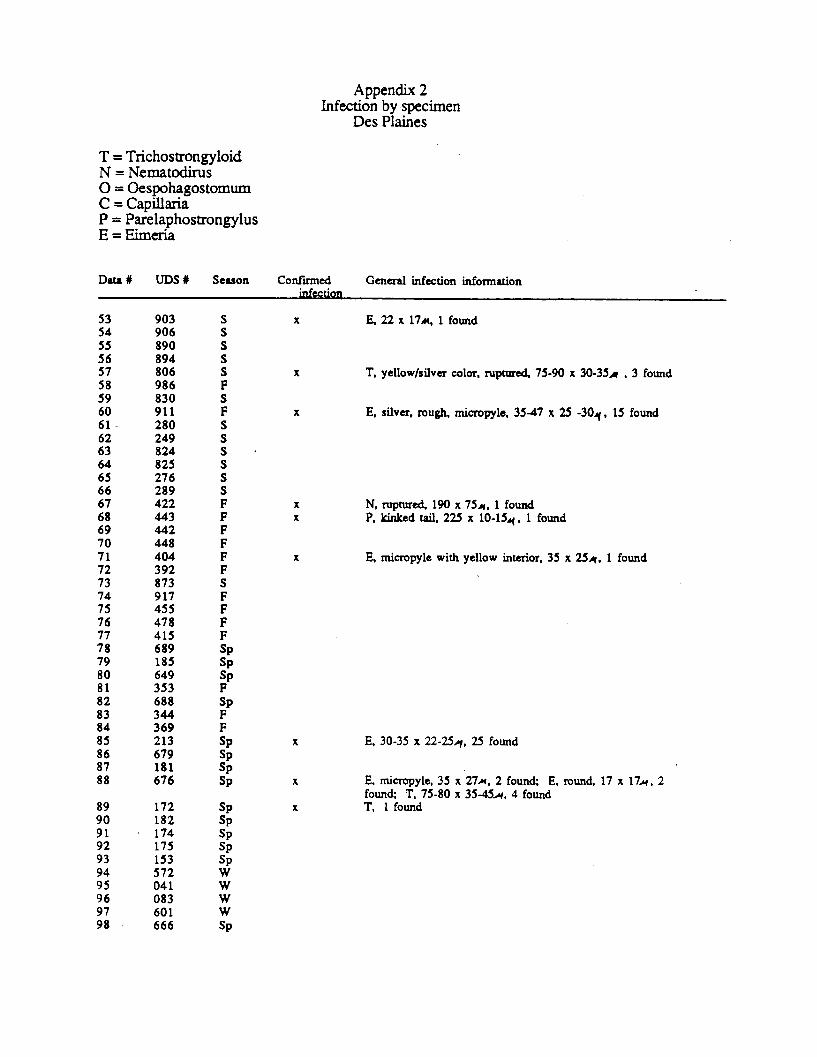
Appendix 2Infection by specimen
Des Plaines
T = TrichostrongyloidN = Nematodirus0 = OespohagostomumC = CapillariaP = ParelaphostrongylusE =Eimeria
Data # UDS # Season Confirmed General infection information---im ion
E, 22 x 17m, 1 found
T. yellow/silver color, ruptured, 75-90 x 3 0-35 A , 3 found
E, silver, rough, micropyle, 35-47 x 25 -3 0A, 15 found
N, ruptured, 190 x 75,., 1 foundP. kinked tail, 225 x 10-154,. 1 found
E, micropyle with yellow interior, 35 x 25q, 1 found
E, 30-35 x 22-25,i 25 found
E, micropyle. 35 x 271, 2 found; E, round, 17 x 17., 2found; T. 75-80 x 35-45,. 4 foundT, 1 found
x
x
x
xx
x
x
x
x
535455565758596061.626364656667686970717273747576777879808182838485868788
89909192939495969798
903906890894806986830911280249824825276289422443442448404392873917455478415689185649353688344369213679181676
172182174175153572041083601666
sssssFSFSSsSSSFFFFFFSFFFF
SpSpSpFSpFF
SpSpSpSp
SpSpSpSpSp
wwwwSpSp

T, 3 foundT, ruptured, 75 x 354, 2 found
E, micropyle, 25 x 204, 1 found
E, 30 x 20-304, 2 foundE, 25 x 20,. 1 found; T, ruptured, 70 x 304, 1 found
99100101102103104105106107108109110
542496568552569544062584585583149549
wwwwwwwwwwSpwW
xx
x
xx

Appendix 3Infection by Specimen
Busse Woods
T = TrichostrongyloidN = Nematodirus0 = OespohagostomumC = CapillariaP = ParelaphostrongylusE = Eimeria
Data # UDS # Season Confirmed General infection informationinfection
111 840 S112 310 S113 239 S x T. 82 x 35,, 1 found; T 65-70 x 40-., 1 found114 836 S x P, kinked tail, 225-240 x 10a, 14 found; T. silver
gray, 80-85 x 40-45v, 2 found115 274 S x E. round, 17 x 174 , 1 found116 299 S117 826 S x E, 25 x 20., 1 found; T, 70 x 374, 1 found118 892 S119 260 S120 . 275 S121 886 S122 895 S x T, ruptured, 80 x 504 , 2 found123 802 S124 815125 871 S126 888 S127 322 S x T, 75 x 35-40.,. 1 found128 2072 W129 829 S x P. 255 x 10q, 3 found130 854 S131 2063 W x T. ruptured, 60 x 35,, 1 found; E, micropyle, 30-35 x
254,. 2 found132 2064 W133 831 S134 905 S x T, ruptured, 75-85 x 35-42A, 29 found; T larvae, 6
found; P. kinked tail, 190-225 x 10-15,4, 6 found135 2049 W136 2056 W137 557 W x T, 80-85 x 40-45., 2 found138 2033 W x E, micropyle, 25-27 x 154,, 1 found139 2070 W x P. 225-250 x 104., 7 found; P. (better condition) 350
x 17,. 1 found; E, 25 x 204, 1 found140 2073 W141 030 W142 036 W143 528 W144 602 W145 024 W146 2020 W x O, 70 x 554, 1 found; T, 70 x 35,, 1 found; P, 1
found147 2027 W148 2028 W149 2038 W x P. 235-250 x 10 -15 A, 3 found150 2059 W151 2055 W x C, 50-55 x 22-25 , 3 found152 2075 W x E, 25 x 154, 1 found153 2022 W154 2037 W x C. 55 x 27.4 1 found; O,.85-90 x 401 , 2 found
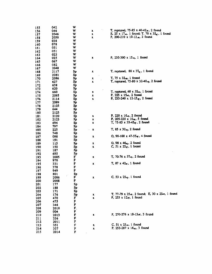
155156157158159160161162163164165166167168169170171172173174175176177178179180181182183184185186187188189190191192193194195196197198199200201202203204205206207208209210211212213214215
04204620462050038078031051023025067082204821172081208662763862066020952114209921056442125212021236947972257480981911151501876952005970331378949801200620081771881711764704753462010004201333620113513572014
wwwwwwwwwwwwwSpSpSpSpSpSpSpSpSpSpSpSpSpSpSpSpSpSpSpSpSpSpSpSpSpFFFFFSpFFSpSpSpSpFFFF.FFFFFFF
xxx
x
x
xx
xxx
xxx
x
x
xx
x
x
x
xx
x
xx
T. ruptured, 75-85 x 40-424, 2 foundE, 25 x 17., 1 found; T, 70 x 35 ,. 1 foundP. 200-210 x 10-12,. 2 found
P. 250-300 x 15.4, 1 found
T, ruptured, 80 x 37. , 1 found
T, 75 x 324, 1 foundT. ruptured, 75-80 x 3 2 -4 0., 2 found
T, ruptured, 60 x 35,q. 1 foundP. 225 x 15U, 2 foundP. 235-240 x 12-15~. 2 found
P, 220 x 10 .q, 2 foundP. 205-220 x 104, 5 foundT, 75-85 x 3 5-4 5, 2 found
T. 85 x 30., 2 found
0, 90-100 x 4 7 -55#, 4 found
0, 98 x 46., 2 foundC, 51 x 25#.. 1 found
T. 70-76 x 37.m. 2 found
T, 87 x 42., 1 found
C, 53 x 25 ,.1 1 found
T, 77-79 x 35.4, 2 found;P, 253 x 124, 1 found
E, 30 x 23m, 1 found
P, 270-276 x 10-13., 3 found
C, 51 x 25,. 1 foundP, 253-287 x 16., 3 found

Appendix 4Infection by Specimen
Non-Cook
T = TrichostrongyloidN = Nematodirus0 = OespohagostomumC = CapillariaP = ParelaphostrongylusE = Eimeria
Data # UDS #
216 975-217 976218 400219 877220 907221 960222 430223 449224 416225 431226 460227 956228 350229 425230 374231 396232 526233 553234 001235 2024236 387237 536238 002239 081240 504241 507242 514243 541244 765245 796246 080247 673248 713249 757250 202251 742252 818253 878254 635255 647256 811257 819258 827259 875260 847261 870262 114
Season
FFFS
FFFFFFFFFFFWWWWFWWWWWWW/SpSpWSpSpSpSpSpSSSpSpSSSSSSSp
Confirmed;ivPrt^mM
xx
xx
x
General infection information
C, 40-46 x 21-23 , 2 foundN, 150-160 x 70-754., 3 found
T, 72 x 40., 1 foundT, 75 x 35q, 1 found
T, 72 x 30.1, 1 found; N, 140 x 531, 1 found
---LLUC;ULILM

263 247 S264 321 S265 843 S266 085 Sp267 820 S x T. 86 x371., 1 found268 119 Sp269 158 Sp270 251 S

Addendum
The original sample inventory submitted for flotation included 274 fecal groups. The final numberexamined was 270. From the original list, six samples were exempted per your request. Three samples,963 (Northwest Cook), 78 and 826 (Busse Woods) were found in the sample bags and were analyzed inplace of three samples, 969 (Northwest Cook), 73 and 876 (Busse Woods) listed on the inventory, but notfound in the bags. Two additional samples (877 and 907, Non-Cook) found in the bags but not listed in theinventory were analyzed.
Appendix F. Witham, J.H., E.A. Cook, and J.M. Jones. No date. White-tailed
deer habitat change in metropolitan northeastern Illinois. Unpub. manuscript.
14pp.

30 June 1990James H. WithamIllinois Natural History Survey8229 N. Carrolton CourtHanover Park, IL 60103708-289-7620
RH: Metropolitan Deer Habitat . Witham et al.
WHITE-TAILED DEER HABITAT CHANGE IN METROPOLITAN NORTHEASTERN ILLINOIS
JAMES H. WITHAM, Illinois Natural History Survey, 607 E. Peabody, Champaign,
IL 61820
ELIZABETH A. COOK, Illinois Natural History Survey, 607 E. Peabody, Champaign,
IL 618201
JON M. JONES. Illinois Natural History Survey, 607 E. Peabody, Champaign, IL
61820
Abstract: Landsat Thematic Mapper satellite data collected in 1985 and 1988
were used to evaluate white-tailed deer (Odocolleus virginianus) habitat in the2
4-county (5,929 km ) Chicago Metropolitan Area (CMA). Thirteen land cover
classes were combined into 5 general deer habitat categories for each date. In
1988, CMA landscape was 6.7% nondeveloped forest, 49.3% heavily vegetated
residential and cropland, 3.3% maintained grass, 39.1% urban and nondeer
habitat, and 1.6% water. County-owned green belt systems, comprising 7.2% of
the metro area, provide permanent habitat where deer concentrate. Percent
development varied from highly urbanized Cook County (75.9%) to more rural Kane
County (29.5%). Less developed Kane and Lake counties sustained highest net
losses (>8%) and net degradation (17-27%) of deer habitat during 1985-1988.
Less developed counties have the greatest opportunity to plan for future
wildlife habitat; more developed counties are closer to minimum threshold
1
Present address: Illinois Department of Conservation, Div. Wild1.
Resources, 524 S. Second St., Springfield, IL 62701.

Wi than
levels of deer habitat and should focus on how deer will be managed on extant
habitats.
J. WILDL. MANAGE. 00(0):000-000
Key words: Chicago, habitat, Illinois, metropolitan. Odocolleus virginlanus,
Landsat thematic mapper, urbanization, white-tailed deer.
White-tailed deer persist in many North American metropolitan areas
because they habituate to human disturbances and because such areas support
diverse plant associations that provide energy and space necessary for deer to
survive and reproduce. Contemporary urban land planners often ameliorate
wildlife habitat by using open space and natural features in their development
concepts (Leedy 1979, Hench et al. 1987); however, many older urban communities
also possess similar features that sustain deer populations. Examples of
typical metropolitan deer habitat are: riparian corridors with buffer
vegetation, widely spaced suburban estates that are heavily vegetated, suburban
arboreta, municipal and county nature centers, remnant agricultural fields, and
manicured grounds surrounding Institutions and corporate buildings.
The Chicago Metropolitan Area (CMA) is comprised of many natural and
cultivated plant associations that are largely determined by land ownerships
(Schmid 1975, Swink and Wilhelm 1979). White-tailed deer are abundant and
widely distributed in the CMA. Greatest concentrations of deer are at
suburban-rural fringes and on large county preserves that are bordered by
suburban development (Witham and Jones 1990). Because urban development
continues to radiate from the city of Chicago, there Is a widespread perception
among local publics and resource managers that deer habitat In the CMA Is
decreasing rapidly.

Wi tham
We used satellite imagery data and geographic information system
technologies to Inventory land cover In 4 counties of metropolitan northeastern
Illinois. Our objectives were to estimate percent and total deer habitat in
the CMA during 1988 and to evaluate net changes in deer habitat from 1985 to
1988.
We thank W. Anderson. C.M. Nixon. and G.C. Sanderson for reviewing the
manuscript. This study was cofunded by the Illinois Department of Energy and
Natural Resources and Federal Aid in Wildlife Restoration Project W-87-R, the
Illinois Department of Conservation, U.S. Fish and Wildlife Service, and the
Illinois Natural History Survey, cooperating.
STUDY AREA AND METHODS
The study area of Cook, DuPage, Kane, and Lake counties in northeastern
Illinois supported a human population of 6.86 million In 1988 (Northeast. Ill.
Plan. Com. 1989). General characteristics of the study area were described
previously (Witham and Jones 1987, 1989). Local climate Is predominantly
temperate continental with cold winters (January x minimum temperature = -10.2
C) and warm, humid summers (July A maximum temperature = 28.5 C). Mean annual
precipitation and snowfall are 89.7 ca and 101.1 ca, respectively (Natl.
Oceanic and Atmospheric Admin. 1987). Soils are derived primarily from glacial
drift and were described to the association level by Fehrenbacher et al.
(1984). On the basis of similarities in physiographic and biotic communities,
Schwegman (1973) included the study area In the Northeastern Morainal Division
of Illinois, except for southwest Kane County, which is in the Grand Prairie
Division. Swink and Wilhelm (1979) documented species, associations, and
distribution of native plants in the Chicago region and Schmid (1975) described
urban vegetation. Upland hardwood forests are dominated by bur oak (Quercus

macrocarpa) and white oak (Q. alba) on dry sites and by sugar maple (Acer
saccharum), basswood (Tilia americana), and red oak (Q. ruba) on mesic sites;
floodplain forests dominants are silver maple (Acer saccharinum) and American
elm (Ulmus americana). Remnant prairie, fen, marsh, and bog communities are
interspersed in the study area. The history and ecology of white-tailed deer
in the midwest agricultural region (Gladfelter 1984) and specifically in
Illinois (Pletsch 1954, Calhoun and Loomis 1974, Nixon et al. 1989) are well
documented.
Landsat Thematic Mapper (TM) data collected 27 June 1988 and 5 June 1985
were selected to inventory land cover and short-term change in land cover. TM
data have a ground resolution of 30 X 30 a (i.e., pixel size = 0.09 ha) with 7
bands of data ranging in the energy spectrum from visible light, to reflective
infrared radiation, to thermal infrared radiation (Iverson and Cook 1988). TN
data sets were geographically referenced to Universal Transverse Mercator (UTM)
coordinates by the use of identifiable ground control points. A supplemental
data set was acquired from Northeastern Illinois Planning Commission which
documented the dominant land use (rural, urban residential, or public open
space) for each quarter section of the township, range, section map reference
system. These data were used to stratify the TM data to aid in classifying
land cover. This step and the subsequent processing described below were
applied to each TM data set, with 1988 used as an example in the description.
An "unsupervised" clustering algorithm, based on means and euclidlan distances
from the mean, identified 195 spectrally distinct pixel clusters. Aggregation
of these clusters into 13 land cover classes was accomplished by studying their
spectral characteristics and their locations on aerial photographs. Sample
points of each land cover class were field checked. Land cover class
descriptions (Table 1) ultimately were based on the commonalities found at the
Withan
sample points. Ambiguous data were isolated in unique classes to maximize
class separation. For example, some confusion existed among alfalfa, sod. and
savanna: these mixed clusters were placed in a separate class from areas
identified exclusively as savanna. The Illinois Geographic Information System
(IGIS, Brigham 1988) was used to subset the data and produce land cover
statistics by counties.
Land cover classes were combined into 5 categories (Table 1) based on
their relative value as whitetail habitat in metropolitan northeastern
Illinois. Nondeveloped forests and savannas were rated as primary deer habitat
because they provide year-round concealment, thermal cover, and forage and
because they are concentration sites for deer during winter in central and
northern Illinois (Nixon et al. 1988). Secondary habitat was land cover that
was favorable for deer, but with some limitations. Field crops were considered
secondary deer habitat due to seasonal availability of food and cover.
Residential estates with tree canopy closure >30% were secondary deer habitat
because unrestricted use of estates by deer is precluded by human disturbances,
physical barriers, and varying human tolerance for deer. We considered
tertiary deer habitat as vegetation that deer would use only if it was proximal
to primary or secondary deer habitat. Urban features (e.g., construction,
nonresidential buildings, parking lots, residential areas without trees, roads)
were regarded as nondeer habitat. Pixels with water signatures were treated
independently because of their ambiguity; open water is not usable, whereas a
vegetated shoreline associated with suitable habitat would be used by deer.
Because we did not censor deer habitat by minimum size or by association with
other habitat types, our estimates represent the maximum potential deer habitat
in the CMA.
5

Witham
We used IGIS techniques to overlay the 1985 and 1988 deer habitat
classifications to detect pixel by pixel changes. The 25 resulting change
categories (i.e., a 5 X 5 matrix) were aggregated to represent 6 potential
outcomes of habitat change: 1) no change, 2) habitat gain, 3) habitat loss, 4)
habitat improvement, 5) habitat degradation, and 6) other. Net change in total
deer habitat was defined as:
habitat gain - habitat loss.
Net change in habitat quality was calculated as:
(habitat improvement + habitat gain) - (habitat degradation + habitat loss)
2The 1988 satellite data did not cover 2.4% (29.31 km ) of northeastern
2Lake County or 0.5% of the 5,929.14 km total study area. This relatively
small amount of unclassified area had virtually no effect on estimates of 1988
land cover or changes in cover between 1985 and 1988.
RESULTS2
More than 50% of the CMA was classified as primary (6.7%, 394.9 km ),2 2
secondary (49.3%, 2,905.7 km ), or tertiary (3.3%, 193.0 km ) deer habitat in2
1988. Trees were present on one-quarter (24.7%, 1,457.2 km ) of the CMA
landscape as nondeveloped forests, savannas, or residential areas with canopy
closure >30%. Percent forest cover in the most urbanized counties of Cook
(29.9%) and DuPage (31.2%) was >2X higher In 1988 than during presettlement in
1820 (Iverson et al. 1989). Secondary deer habitat was 83.2% of all deer2
habitat; nondeer habitat and water comprised 39.1% (2,308.9 km ) and 1.6% (97.02
km ) of the CMA, respectively.
The 4 counties represented a gradient of urbanization. Cook County was

Witham2
most developed with 75.9% (1.880.1 km ) In forested residential or urban land2 2
cover. DuPage (65.5%, 570.6 km ), Lake (43.6%, 520.2 km ), and Kane (29.5%.,2
400.3 km ) counties were progressively less developed. Percent deer habitat
within counties was an inverse gradient of urbanization with values ranging
from 44.8% (Cook County) to 77.0% (Kane County). Because It is almost 2X
larger than other CMA counties, Cook County had the most area In deer habitat2
(1,111.1 km ) despite having the lowest percent deer habitat among counties.2 2
Both Lake (819.4 km ) and DuPage (517.7 km ) counties had less total deer
habitat than Cook or Kane counties (Table 2).
With 1 exception, all counties sustained net reductions In deer habitat
and deer habitat quality from 1985 to 1988 (Table 3). Percent net losses of2
deer habitat were highest in more rural counties of Kane (-8.7%, 117.9 km ) and2 2
Lake (-8.3%., 99.5 km ) and lowest in DuPage County (-4.7%, 40.84 km ). An
increase in secondary deer habitat in Cook County contributed to a modest net2
gain (1.4%, 33.7 ka ) in total deer habitat. CMA counties sustained net losses2
of deer habitat totalling 242.0 km (-4.1% of CMA) during the 3-year period2 2
evaluated. DuPage County (-15.3%, 133.3 km ) and Kane County (-16.2%, 219.6 km )2
experienced moderately high, and Lake County (-27.0%, 323.0 km ) very high,
reductions in deer habitat quality. In Cook County, habitat quality decreased2
at a more modest rate (-4.9%, 120.7 km ).
DISCUSSION
Deer habitat classifications used in this study reflect macro habitat
types available to deer within the CMA. Such classification does not Indicate
actual deer use or densities as both will vary within classes because of site
specific differences in plant community composition and structure. Other
factors such as habitat Interspersion, deer behavior, human disturbances, plant

Withaa
phenology, soils, and weather also influence temporal and spatial distributions
of whitetails. Thus, our habitat evaluation represents potential deer habitat
and is most useful for broad-scale comparisons between relatively distinct
types (e.g., forested vs. urban features, developed vs. nondeveloped).
The perception that deer habitat was declining in the CMA was accurate,
particularly in the more rural Lake and Kane counties where percent habitat
loss and degradation were highest. Rapid loss of deer habitat displaces some
deer and may contribute to higher rates of mortality, dispersal or wandering,
and/or increased deer densities on suitable remaining habitat. Deer numbers
increased statewide in Illinois during the 1980's, but the exponential increase
in deer-vehicle accidents (Illinois Dep. Trans., unpub. data), high numbers of
complaints of deer browsing damage to ornamental plants, and locally severe
degradation of plant communities on remnant natural areas in the CMA (Witham
and Jones 1987) may be exacerbated by deer that have been displaced by habitat
degradation or loss.
The declining trend in total deer habitat that occurred during 1985-1988
will not result in long term elimination of deer habitat in the CMA because
large tracts of natural and restored plant communities are permanently
protected in open space properties owned by county forest preserve districts
(Wendling et al 1981, Witham and Jones 1987). These forest preserves covered
approximately 7% of the CMA In 1988, (11 of Cook County, 9% of DuPage County,
4% of Lake County, and 1% of Kane County). All forest preserves were not
suitable deer habitat as some properties were designated for recreational and
educational uses. However, deer are able to utilize most of the available
resources on preserves that receive intensive human use because they tend to
habituate to human disturbances.
8

Witham
Although Kane County ranked highest (77.1%) in percent deer habitat among
counties, It was depauperate in nondeveloped forest cover (3.6%) compared to
Cook (8.1%) and Lake (8.2%) counties. Differences among counties in the
relative amount of primary to seasonal habitats suggest that deer, particularly
in Cook and Kane counties, may require different strategies for using resources
of these counties. In Illinois, farmland deer concentrate in protected
woodlots during winter and then disperse or migrate into agricultural areas
during spring and early summer (Nixon et al. 1988, 1989). Most deer are
eliminated from agricultural fields and small woodlots in winter by harvest of
crops, by regulated hunting, and through annual migrations to more secure
habitats. Although firearm hunting is not permitted in Kane County, the
dominance of cropland (51%) and limited nondeveloped forest cover creates a
similar habitat repletion-depletion cycle where deer must migrate seasonally to
and from the larger forests for winter protection.
In contrast to Kane County, Cook County had more nondeveloped forested
cover (8.1%) and only limited seasonal cropland (4.7%). Urbanization has
increased the Insularity of primary deer habitat in Cook County, thus, in many
areas deer must negotiate diverse barriers to use disjunct secondary habitats
(i.e., cropland). Although dispersal by some subadult whitetails is likely,
the limited availability of cropland and the potential costs of injury or
mortality Incurred by deer attempting to travel through "high risk" urban areas
to scattered croplands precludes such movements by most CMA deer. The
relatively low mobility of Cook County deer is supported by observations of 12
radio-collared adult and yearling does that were captured and released in Cook
County during 1984; none was observed to migrate or disperse (Jones and Witham,
unpub. data). Conservative movements by deer in highly developed metropolitan
Wi than
areas, such as Cook County where 5.3 million people reside, may be typical and
perhaps selected for through differential survival that favors deer that are
more sedentary.
MANAGEMENT IMPLICATIONS
Deer habitat included land use classes with different potentials for
development, which may have large scale effects on future distributions and
abundance of whitetails in the CMA. Cover for deer on residential areas with
>30% canopy closure is predictably more stable than cover on agricultural land
in suburban-rural fringe areas which have high potential for conversion to
nondeer habitat. In Cook and DuPage counties, secondary deer habitat was
mostly (64% and 53%, respectively) forested residential areas. In contrast,
secondary deer habitat in more rural Lake and Kane counties was predominantly
in less stable cover such as cropland (71% and 90%, respectively).
Counties that are least developed have the greatest flexibility and
potential for choosing the amount, distribution, and design of wildlife
habitats within their Jurisdictions (Hench et al. 1987). Protection of
wildlife habitat can be achieved through county and municipal zoning (Bissell
et al. 1987) or through purchase of properties for nondevelopment or
restoration of natural vegetation. Presently, Kane and Lake counties have the
greatest opportunity to plan for wildlife habitat on their developing
metropolitan landscapes. Future abundance and distribution of deer in Kane and
Lake counties will depend on if, and how, current land use plans (e.g., Byers
et al. 1987) are enacted. Concomitant with retention or restoration of
wildlife habitat on developing landscapes is recognition that adverse deer-
human interactions will increase and will require counties, municipalities, and
10

Witham
publics to be more directly involved in local deer management (Witham and Jones
1989).
In contrast, deer habitat in Cook County, and to a lesser degree in DuPage
County, is in more permanent cover. Forest preserves comprise 8.7-11% of these
counties and provide minimum thresholds of inviolate deer habitat. Secondary
deer habitat is predominantly (21.8-25.9% of total county area) in heavily
treed residential areas, which tend to become more vegetated over time.
Because deer habitat in these urbanized counties is in more stable land use
types than in rural counties, fewer opportunities exist for changing such
habitats through large scale landscape modifications. Natural resource
managers, administrators, and publics in these urbanized counties should
clearly define site management objectives for existing habitats and decide how
deer and other wildlife species will be managed to meet these objectives.
LITERATURE CITED
Bissell, S.J., K. Demarest, and D.L. Schrupp. 1987. The use of zoning
ordinances in the protection and development of wildlife habitat. Pages 37-
42 in L.W. Adams and D.L. Leedy, eds. Integrating man and nature In the
metropolitan environment:proceedings of a National Symposium on Urban
Wildlife. Chevy Chase, Maryland.
Brigham, W. 1988. Illinois Geographic Information System. Ill. Nat. Hist.
Survey Reports. Nos. 281, 282.
Byers, S.M., R.A. Montgomery, and G.V. Burger. 1987. An assessment of
wildlife and wildlife habitat in Kane County, Illinois. Page 238 in L.W.
Adams and D.L. Leedy, eds. Integrating man and nature in the metropolitan
environment: proceedings of a national symposium on urban wildlife. Chevy
Chase, Maryland.
11

Wi than
Calhoun, J., and F. Loomls. 1974. Prairie whitetails. Ill. Dep. Conserv.,
Springfield. 50pp.
Fehrenbacher, J.B., JD. Alexander, I.J. Jansen, R.G. Darmody, R.A. Pope, M.A.
Flock, E.E. Voss, J.W. Scott, W.F. Andrews, and L.J. Bushue. 1984. Soils
of Illinois. College of Agric. Bull. 778. Univ. Ill., Champaign-Urbana.
85pp.
Gladfelter, H.L. 1984. Midwest agricultural region. Pages 427-440 in L.K.
Halls, ed. White-tailed deer ecology and management. Stackpole Books,
Harrisburg, Penn.
Hench. J.E., K.V. Ness, and R. Gibbs. 1987. Development of a natural
resources planning and management process. Pages 29-35 In L.W. Adams and
D.L. Leedy, eds. Integrating man and nature in the metropolitan
environment: proceedings of a National Symposium on Urban Wildlife. Chevy
Chase, Maryland.
Iverson, L.R., and E. A. Cook. 1988. Can the productivity of Illinois forests
be estimated from space? Ill. Nat. Hist. Survey Reports. No. 273.
Iverson, L.R., R. L. Oliver, D.P. Tucker, P.G. Risser, C.D. Burnett, and R.G.
Rayburn. 1989. The forest resources of Illinois: an atlas and analysis of
spatial and temporal trends. Ill. Nat. Hist. Survey Special Pub. 11. 181pp.
Leedy, D.L. 1979. An annotated bibliography on planning and management for
urban-suburban wildlife. Fish and Wildlife Service, U.S. Dep. Interior
FWS/OBS-79/25. 256pp.
National Oceanic and Atmospheric Administration. 1987. Local climatological
data, annual summary, Chicago O'Hare International Airport, Illinois. U.S.
Dep. Commerce, Natl. Climatic Data Center, Ashevllle, North Carolina.
12

Witham
Nixon, C.M., L.P. Hansen, and P.A. Brewer. 1988. Characteristics of winter
habitats used by deer in Illinois. J. Wildl. Manage. 52:552-555.
, and J.E. Chelsvig. 1989. Illinois deer
investigations: Life history and ecology of white-tailed deer In an
intensively farmed region of Illinois. Ill. Dep. Conserv., Fed. Aid Wild1.
Restor. Final Rep. W-87-R-8,9,10. 124pp.
Northeastern Illinois Planning Commission. 1989. The components of population
change in northeastern Illinois 1980 to 1988. Data Bull. 89-4. Northeast.
Ill. Plan. Comm., Chicago. 6pp.
Pietsch, L.R. 1954. White-tailed deer populations in Illinois. Biol. Note 34.
Ill. Nat. History Survey, Urbana. 22pp.
Schmid, J.A. 1975. Urban vegetation, a review and Chicago case study. The
Univ. of Chicago Dep. of Geogr. Res. Paper No. 161. Illinois. 266pp.
Schwegman, J.E. 1973. Comprehensive plan for the Illinois Nature Preserves
System, Part 2, The natural divisions of Illinois. Ill. Nat. Pres. Comm.,
Springfield. 32pp.
Swink, F., and G.S. Wilhelm. 1979. Plants of the Chicago region. Third ed.
The Morton Arboretum, Lisle, 11. 922pp.
Wendling, R.C., S.J. Gabriel, J.F. Dwyer, and R.L. Buck. 1981. Forest
Preserve District of Cook County, Illinois. J. For. 79:602-605.
Witham, J.H., and J.M. Jones. 1987. Deer-human Interactions and research in
the Chicago Metropolitan Area. Pages 155-160 in L.W. Adams and D.L. Leedy,
eds. Integrating man and nature in the metropolitan environment. Natl.
Inst. for Urban Wildl., Columbia, Md.
13

Wi tham
____ and ________. 1989. Managing urban deer in Illinois: the role
of state government. Pages 81-84 in A.J. Bjugstad, D.W. Uresk, and R.H.
Haare, eds. Ninth Great Plains Wildl. Damage Control Workshop Proceed.,
Gen. Tech. Rep. RM-171, U.S. Dep. Agric., Fort Collins, Colo. 181pp.
,_ and . 1990. White-tailed deer abundance on
metropolitan forest preserves during winter in northeastern Illinois.
Wildl. Soc. Bull. 18:13-16.
Received
Accepted
14
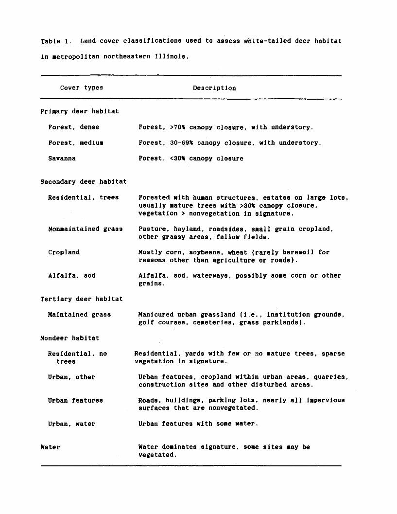
Table 1. Land cover classifications used to assess white-tailed deer habitat
in metropolitan northeastern Illinois.
Cover types
Primary deer habitat
Forest, dense
Forest, medium
Savanna
Secondary deer
Residential,
habitat
trees
Nonmaintained grass
Cropland
Alfalfa, sod
Tertiary deer habitat
Maintained grass
Nondeer habitat
Residential, notrees
Urban, other
Urban features
Urban, water
Water
Description
Forest, >70% canopy closure, with understory.
Forest, 30-69% canopy closure, with understory.
Forest, <30% canopy closure
Forested with human structures, estates on large lots,usually mature trees with >30% canopy closure,vegetation > nonvegetation in signature.
Pasture, hayland, roadsides, small grain cropland,other grassy areas, fallow fields.
Mostly corn, soybeans, wheat (rarely baresoll forreasons other than agriculture or roads).
Alfalfa, sod, waterways, possibly some corn or othergrains.
Manicured urban grassland (i.e., institution grounds,golf courses, cemeteries, grass parklands).
Residential, yards with few or no mature trees, sparsevegetation in signature.
Urban features, cropland within urban areas, quarries,construction sites and other disturbed areas.
Roads, buildings, parking lots, nearly all impervioussurfaces that are nonvegetated.
Urban features with some water.
Water dominates signature, some sites may bevegetated.

LA N '- 04
s N 40?Cm o » (
NM 4
44 NMc» -
LA
0
0 44- 4004 CN
L
0
44
I'I
I-J
Ii6
I
C
4,
L
S
4.4
C-S
N
S
S4-
0 o04 (0
r- LA L A
4- 0- LA 0
C4
LA LA » 0404 - 4 4-
('4 N;
-
0Ln40
Ln4
Ln
CT»0V
U,
40 in L 0
04 CM (Oo» wr (
q4-
40 LA 0
LA1)
6 6
lb 0 4
II
*0 0m N(w)
6*1 toN 0oco
- N
4 N^
N^ NNw
40 r- LA 0 4
4r- 4- 40 0o 4UM ND V C4 f
N N
0» 4-
4» LM
4,4 4,44, M
Vy 0o C L04 4 Ln
('4 NM 4
40 4
04 04
SV- 0 P oNM P. NM 0 0
LA» 04 L 00 M0 0 0 D
4- oLA - C NDLA 00 0 0
04
C4
NM -4- LA
0- o04» (4
N 0
S
C-S
'4C-S
0 0
OD 0(44 00
N< ^
0
0440
LAp--
0
0C40N
LA §
0o
U$-
N
(444
404
N
S(4440
U
N
S
Ci
N
S
'4- '4
U
-- C 0 NM 0 CNM C4 a 04
Ln
0
tO
u
U44
C;orý»
C44
0
Ch
0
c-
0
> 0
ou
I
II
0
A
S
o
Q.
040
40LA
(4404>
CM
44S44
I
C.
L
S
S
i'4
2
I
>u
j

Table 3. Percent change in deer habitat from 5 June 1985 to 27 June 1988 for
Cook, DuPage, Kane, and Lake counties, Illinois.
% Change By CountyChanges In deer habitat
during 1985 and 1988 Cook DuPage Kane Lake
Habitat gain (GAIN)(non habitat or water -- habitat)
Habitat loss (LOSS)(habitat --. non habitat or water)
Habitat Improvement (IMPROVED)(tertiary -- secondary or primary)(secondary -> primary)
Habitat degradation (DEGRADED)(primary -- secondary or tertiary)(secondary -> tertiary)
Net change In habitat(GAIN - LOSS)
Net change in habitat quality(IMPROVED + GAIN) - (DEGRADED + LOSS)
10.45 9.66 4.41 6.28
9.09 14.35 13.10 14.61
1.68 4.11 1.73 2.15
7.91 14.73 10.06 20.86
+1.36 -4.69 -8.69 -8.33
-4.87 -15.31 -17.02 -27.04

Appendix G. Jones, J.M., and J.H. Witham. 1990. Post-translocation survival
and movements of metropolitan white-tailed deer. Wildl. Soc. Bull. 434-441.

i * .l 9
R114D
Wildl. Soc. Bull. 18:434-441, 1990
POST-TRANSLOCATION SURVIVAL AND MOVEMENTSOF METROPOLITAN WHITE-TAILED DEER
JON M. JONES,' Illinois Natural History Survey, 607 E. Peabody Dr., Champaign, IL 61820
JAMES H. WITHAM, Illinois Natural History Survey, 607 E. Peabody Dr., Champaign, IL 61820
Problems associated with large concentra-tions of white-tailed deer (Odocoileus virginia-nus) are accentuated in metropolitan areaswhere herds are isolated within preserves orparks by urban development. The resultantreduction in plant species richness and struc-ture on these natural areas, adverse effects uponother wildlife species (e.g., ground nesting spe-
SPresent address: Illinois Department of Conserva-tion, Division of Wildlife Resources, 524 S. Second St.,Springfield, IL 62701.
cies), deer-vehicle accidents, and damage toornamental plants on private properties nearpreserves can increase to undesirable levels(Decker and Purdy 1988) and can eventuallyrequire site-specific population reduction.However, segments of the urban public opposemethods that involve the killing of deer(Heintzelman 1988) and advocate translocat-ing deer from metropolitan environs to morerural settings (Nielsen 1988).
Palmer et al. (1980) and Ishmael and Rong-stad (1984) demonstrated that lethal deer pop-

SURVIVAL OF TRANSLOCATED DEER * Jones and Witham 435
ulation reduction techniques (i.e., closely reg-ulated public hunting and sharpshooting overbait, respectively) were most effective in termsof manhours and cost per deer removed. How-ever, cost and time required to live captureand translocate deer appear to be secondaryconcerns to many metropolitan residents whooppose lethal methods and view translocationas a means of "saving" individual deer whileaddressing the problem of reducing deer num-bers. The measurement of "survival" is essen-
tial for assessing success if the objective fortranslocation is to save the lives of individualanimals. Studies on the post-translocation sur-vival of nutritionally stressed black-tailed deer(0. hemionus) (O'Bryan and McCullough1985), genetically superior white-tailed deer(McCall et al. 1988), and free-ranging ruralwhite-tailed deer (Hawkins and Montgomery1969, Pais 1987) indicate that a substantialnumber of deer will die during capture, trans-location, or shortly after release; however, nostudies have evaluated the survival of white-tailed deer translocated from metropolitan torural areas.
As part of a 6-year study of white-tailed deerin the Chicago Metropolitan Area, we moni-tored the fates of deer captured on metropol-itan preserves and translocated to a rural lo-cation. The objectives of this study were tomonitor the survival of translocated deer dur-ing the first year post-release and to comparethe survival and movements of translocateddeer to the survival and movements of deerthat were captured and marked, but not trans-located from metropolitan preserves.
STUDY AREAS
Metropolitan Capture Sites
White-tailed deer were captured during the wintersof 1984-1988 from 3 locations within Cook County,Illinois: the 1,499-ha Ned Brown Preserve (Ned Brown),the 1,242-ha Des Plaines Preserve (Des Plaines), andthe 900-ha Chicago-O'Hare International Airport(O'Hare). Cook County is one of the largest counties(2,480 km 2) in Illinois (Neely and Heister 1987) and
the most highly populated with >5.2 million residentsin 1988 (Northeast. 11. Planning Comm. 1989). Allmetropolitan area capture sites were in townships with>77,000 residents (U.S. Census Bureau, unpubl. data).The 18,055 km of roads in Cook County sustain > 124.3million average daily vehicle-kilometers of travel (Ill.Dep. Trans., 1988, unpubl. data). Based on Landsatsatellite imagery data, 33% of Cook County was inurban or suburban land use classes in 1985 (E. Cook,Ill. Nat. Hist. Surv., Champaign, pers. commun.).
Ned Brown typifies all capture sites in that majorhighways dissect or border deer habitat and adjacentproperties are extensively developed. Ned Brown sus-tains intensive public use with > 1.5 million visitorsannually (Dwyer et al. 1985). Cover types are: 66% inwoodlots dominated by oak (Quercus spp.), sugar ma-ple (Acer saccharum), and basswood (Tilia americana),10% in old field successional stages, wetlands, andmowed grass, 15% in open water, and 9% in roads andother developments. Deer density during the winter of1984 was >20/km2 (Witham and Jones 1990).
Des Plaines differs from Ned Brown in that the for-mer is riparian habitat with woodlots dominated bysugar maple and basswood. O'Hare differs in that deerhabitat consists of early second growth (i.e., mostlyshrubs and saplings) woodlots and grassy areas or earlysuccessional fields adjacent to runways. A minimum of7.3 deer/km2 was initially present on O'Hare (Withamand Jones, unpubl. data).
Rural Release Site
Deer were released on the 1,440-ha Joliet ArmyTraining Center, Will County, Illinois. Will Countyencompasses 2,197 km2 (Neely and Heister 1987) with17% of the county in urban or suburban land use (E.Cook, Ill. Nat. Hist. Surv., pers. commun.) and a 1988human population of 346,700 (Northeast. Ill. PlanningComm. 1989); the release site was in a township with4,820 residents (U.S. Census Bureau, unpubl. data). The4,470 km of roads in Will County averaged 9.9 millionvehicle-kilometers of travel daily (Ill. Dep. Trans., 1988,unpubl. data). Relative to Cook County, Will Countyhad 93% lower human population, 77% less urban/suburban development, and 75% fewer kilometers ofroads with 92% less traffic volume.
The Army Training Center is characterized by 540%in mature second growth oak woodlots and 260% inhawthorn (Crateagus spp.) thickets and old fields. Hu-man activity on the training center is restricted to mil-itary training exercises, occasional construction activ-ities, a 6-day shotgun harvest of deer (3 days each inNov and Dec), and a 3-month (Oct-Dec) archery sea-son for deer. Two-lane roads surround most of thetraining center but have less vehicular traffic than themany 4-lane highways near the capture areas. Limitedresidential development, industrial complexes situatedon large acreages, and a 9,400-ha U.S. Army ammu-nition plant are contiguous with the training center.Security fences which surround most of the industrial

436 Wildl. Soc. Bull. 18(4) 1990
and military areas are partial barriers to deer move-ments. The training center is 580 km (straight line)from the capture sites and had a minimum density of5 deer/km2 during the winter of 1988 (111. Dep. Con-serv., unpubl. aerial counts).
METHODS
Deer were captured with rocket nets (Hawkins et al.1968). Exceptions were 2 deer that were captured withdrive nets (Silvy et al. 1975) and 1 deer captured byremote chemical injection (Jessup and Hunter 1989).Once captured, deer were manually restrained, blind-folded, and sedated with 8 mg/kg ketamine hydro-chloride (Ketaset, Bristol Laboratories, Syracuse, N.Y.)and 1 mg/kg xylazine hydrochloride (Rompun, MilesLaboratories, Shawnee, Kans.). All animals were agedby tooth wear and replacement as either fawns (5 1 year)or adults (> 1 year) (Severinghaus 1949). Yearling doeswere included in the "adults" category due to the smallnumber of yearlings captured. Each doe was markedwith a metal ear tag (National Band and Tag Co.,Newport, Ken.) in each ear, a numbered white plasticcattle tag (Y-TEX Corp., Cody, Wyo.) in the right ear,and a standard radio collar with a mortality sensor(Telonics, Inc., Mesa, Ariz.). Bucks were marked sim-ilarly but were not radio-collared. Deer to be translo-cated were placed in individual transport crates orcollectively in a completely darkened horse trailer. Yo-himbine hydrochloride (Sigma Chemical Co., St. Louis,Mo.), which acts as an antagonist of Ketaset and Rom-pun (Jessup et al. 1983, Mech et al. 1985), was admin-istered intravenously at 0.15 mg/kg prior to transport;animals were alert upon reaching the release site. Res-ident does released at capture sites in Des Plaines dur-ing March-April 1984 were marked similarly but werenot sedated nor tagged with cattle tags.
Radio-collared deer were relocated with truck-mounted, paired, 4-element Yagi antennae attached toa portable receiver. A null-peak system was used todetermine bearings. Resident does were relocated ev-ery 1 to 2 weeks. Translocated does were relocatedevery 2 weeks during the first 6 months of 1985, butrelocation intervals were extended to once a month orevery other month when long-distance movements didnot occur. Individual animals that moved from therelease site were relocated more frequently until it wasapparent that the animal had settled into a new areaor returned to the release area. Telemetry system ac-curacy was evaluated by triangulating the locations,unknown to the researcher doing the triangulations, ofradio transmitters placed in Ned Brown. The systembias and precision (SD) were calculated according toLee et al. (1985). The system bias was 0.1* (SD = 8.4*)at s2.6 km.
The MICROMORT computer program (Heisey andFuller 1985) was used to calculate seasonal and annualsurvival rates for all collared deer and cause-specificmortality rates for translocated does. In order not to
violate the assumptions of MICROMORT, the first yearpost-release was divided into 4 seasons. All translocatedanimals were released during the winter season (18Dec-31 Mar) which started after the annual shotgunharvest of deer in December but included the last 14days of the annual harvest by archers. Subsequent sea-sons included the spring fawning season (1 Apr-30 Jun),summer (1 Jul-30 Sep), and the autumn hunting season(1 Oct-31 Dec). Accordingly, first year post-releaserefers to a span of 9-12 months; annual survival cal-culated for animals translocated in January-March rep-resents a time span less than 1 full year. For the residentdeer, the period of capture approximated.the springseason described for the translocated animals; there-fore, the last seasonal rate evaluated for resident deerwas winter of the following year. The number of daysper season ranged from 91 to 103 for the translocateddoes and 90 to 122 for the resident does. Annual sur-vival rates between groups and age classes were statis-tically compared using "z-scores" as outlined by Heisey(1985). The percent survival of ear-tagged, translocatedbucks was empirically calculated based on reports ofknown mortalities.
The survival of does translocated during 4 consec-utive winters was calculated as aggregate seasonal andannual rates. Although seasonal survival rates were sig-nificantly different between years (for both fawns andadults), these interannual comparisons were based onvery small sample sizes per season (i.e., the number ofanimals present at the beginning of a season/intervalranged from 0 to 6). However, pooling of seasonal andannual rates was based on the premise that stress in-curred during capture and transport and mortality fac-tors specific to the release site were comparable amongyears. Although 100 firearm deer permits have beenissued annually at the Joliet Army Training Center,other known decimating factors at the release site var-ied among years. The average daily vehicle-kilometersof travel for Will County increased 8% from 1984 to1988 (Ill. Dep. Trans., 1988, unpubl. data), and annualsnowfall ranged from 40.6 cm in 1986 to 94.5 cm in1985. Average monthly minimum temperatures duringthe 4 winters ranged from -13.1 C to -7.6 C duringJanuary, from -10.6 C to -3.3 C during February,and from -5.7 C to -0.3 C in March.
We used the TELEM computer program (developedby G. Koeln, Ducks Unlimited, Inc., and adapted foruse on personal computers by the Geographic Re-sources Center, University of Missouri-Columbia) tocalculate general indices of post-release movement forrelative comparisons: noncircular home range/annualarea of use, mean activity radius, and longest distancebetween the release site and subsequent radio locations.The latter value was hand calculated from UniversalTransverse Mercator (UTM) coordinates generated byTELEM. Standard transformations of the data failedto approximate normal distributions; thus, movementindices were statistically compared between groups andage classes (release site only) with the Kruskal-Wallisrank test (Proc MRANK; Statistical Analysis System;Sarle 1983).

SURVIVAL OF TRANSLOCATED DEER * Jones and Witham 437
RESULTS
Twenty-five does (13 adults, 12 fawns) weretranslocated during December-March 1984-1988. Among these does, 15 were captured atNed Brown, 5 at Des Plaines, and 4 at O'Hare.One fawn, darted in April 1986 by ChicagoAnimal Control personnel in southeast CookCounty, also was released on the training cen-ter. Nineteen does were moved via individualwooden capture crates and 6 were translocatedby horse trailer. Twenty-five bucks (7 adults,4 yearlings, and 14 fawns) were also moved tothe center. Twelve resident does (9 adults and3 yearlings, categorized collectively as adults)were monitored at Des Plaines during 1984-1987.
Survival rates were calculated for 22 trans-located does (12 adults and 10 fawns) and 12resident does. Three translocated deer weredropped from survival analyses due to trans-mitter malfunction (n = 1 adult doe) and lossof radio collars (n = 2 fawns). Total radio-daysper season ranged from 384 to 668 for trans-located fawns, from 514 to 729 for translocatedadults, and from 861 to 1,095 for resident deer.Accurate determinations of dates and causesof death of translocated does were possible dueto prompt reporting by military personnel,hunters, and motorists. Cause-specific mortal-ity rates were not calculated for the residentdoes because causes of death could not be de-termined in all cases.
Area of use data were deleted for 5 animals(2 translocated fawns, 2 translocated adults,and 1 resident adult) having <4 radio-fixeseach during their first year post-release and forwhich TELEM could not calculate a noncir-cular home range from the available telemetrydata. Therefore, post-release movements wereanalyzed for a total of 21 translocated (11 adultsand 10 fawns) and 11 resident adult does. Al-though all radio locations were used for sur-vival analyses, only 153 locations (triangulat-ed) of resident does (f = 13 locations/doe,range =- 9-17), and 206 locations (triangulated
1.0
0.8
a 0.6
I§ 0.4
0.2
0.0
* Translocated Adults* Translocated FawnsE Resident Adults
H
Season'UUITIUmn
Fig. 1. Seasonal survival for 22 translocated, white-tailed does (12 adults and 10 fawns) of known fatesand 12 resident does in the Des Plaines Preserves, CookCounty, Illinois. Mortality rates shown were calculatedusing the MICROMORT computer program (Heiseyand Fuller 1985).
and observed) of translocated does (f = 9 lo-cations/doe, range = 4-17) during the firstyear post-release were usable under the con-straints of TELEM.
Deaths of translocated deer were catego-rized as vehicle accidents, hunting, and un-known causes (presumably capture myopa-thy). Each cause contributed to a lower survivalrate among translocated deer during the firstseason post-release; estimated survival rates fortranslocated adults and fawns during Decem-ber-March were 0.56 and 0.58, respectively(Fig. 1). Estimated fawn survival increased to0.76 in the spring (Apr-Jun) followed by nodeaths among the fawns (n = 6) surviving thefirst 6 months post-release. Two of the 7 (29%)translocated adult females that survived theinitial translocation and the subsequent springand summer seasons were killed by huntersduring autumn. Three of the 12 resident doesdied during the first year; the estimated sur-vival rate for resident adults was 20.89 during

438 Wildl. Soc. Bull. 18(4) 1990
Table 1. Annual areas of use (AAU), activity radii (AR), and longest distances from capture/release site (DIST)for resident female white-tailed deer (released at their capture site) on a metropolitan forest preserve in CookCounty, 11. and for does translocated from metropolitan preserves to rural habitat in Will County, I11.
AAU (ha) AR (m) DIST (m)
Area/age class n i SE f SE i SE
ResidentAdults 11 253 34 495 45 1,316 154
TranslocatedAdults 11 747 239 698 98 2,411 608Fawns 10 1,793 442 1,199 179 4,373 901
each season. The estimated annual survival ofresident adults (0.73, n = 12) was higher (z =2.01, P = 0.02) than for translocated adults(0.34, n = 12). The annual survival of trans-located fawns was 0.44 (n = 10) and was notdifferent (z = 0.43, P = 0.33) from the survivalrate of translocated adults. Twelve (48%) trans-located bucks were known to have died duringthe first year post-release; 11 (2 adults, 2 year-lings, and 7 fawns) of these were shot by hunt-ers.
Translocated does had higher but not sig-nificantly different (P > 0.05) mean values forannual area of use, activity radius, and longestdistance from the release site than the residentdoes (Table 1). The mean annual area of usepost-release for resident adults (253 ha) wasapproximately one-third of the average areaused by translocated adults (747 ha) but washighly variable among individuals of eachgroup. Although fawns appeared to exhibitgreater movements post-release than oldertranslocated deer, the observed values did notdiffer (P > 0.05).
Seven (32%, 5 fawns and 2 adults) of 22translocated does of known fates moved 25km from the release site during the first yearpost-release. The longest movement from thetraining center was recorded for 1 fawn, cap-tured in southeast Cook County, which in 2months traveled 243 km (straight-line) fromthe release site to within 4 km of its capturesite. Another doe, translocated as a fawn, moved215 km in May-June during 3 consecutive
years to a small woodlot near a rural town butreturned to the army ammunition plant afterthe hunting season.
DISCUSSION
Survival of translocated deer (Odocoileusspp.) has been documented in other studies(Table 2). Direct comparisons of these studiesare complicated by differences between sites,methods of translocation, and methods of cal-culating and reporting survival rates. Thesedata suggest, however, that the survival oftranslocated deer is contingent upon captureand handling procedures, the nutritional statusof the animals, and the presence of decimatingfactors at the release site including hunters,vehicular traffic, predators, or a combinationof these. Additional considerations are habitatquality, density of resident deer at the releasesite, and resultant negative interactions (e.g.,competition for resources, transmission of dis-eases or parasites) between translocated andresident deer.
Capture-related stress, accidents with ve-hicles, and losses to hunters were the majordecimating factors that led to lower survivalamong our translocated does. Capture myopa-thy can affect animals up to 1 month after livecapture (Bartsch et al. 1977, Harthoorn 1977)and was presumably the cause of 3 (12%, 2adults and 1 fawn) mortalities among ourtranslocated does within 0.8 km of release siteduring the first month post-release. Site- and
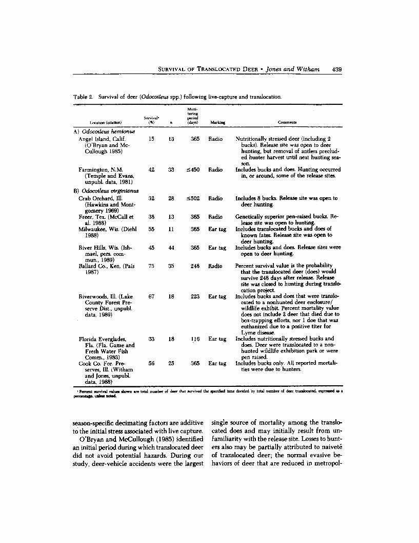
SURVIVAL OF TRANSLOCATED DEER * Jones and Witham 439
Table 2. Survival of deer (Odocoileus spp.) following live-capture and translocation.
Moni-toring
Survival* periodLocation (citation) (%) n (days) Marking Comments
A) Odocoileus hemionusAngel Island, Calif.
(O'Bryan and Mc-Cullough 1985)
Farmington, N.M.(Temple and Evans,unpubl. data, 1981)
B) Odocoileus virginianusCrab Orchard, Il1.
(Hawkins and Mont-gomery 1969)
Freer, Tex. (McCall etal. 1988)
Milwaukee, Wis. (Diehl1988)
River Hills, Wis. (Ish-mael, pers. com-mun., 1989)
Ballard Co., Ken. (Pais1987)
Riverwoods, Ill. (LakeCounty Forest Pre-serve Dist., unpubl.data, 1989)
Florida Everglades,Fla. (Fla. Game andFresh Water FishComm., 1983)
Cook Co. For. Pre-serves, 11. (Withamand Jones, unpubl.data, 1988)
15 13 365 Radio Nutritionally stressed deer (including 2bucks). Release site was open to deerhunting, but removal of antlers preclud-ed hunter harvest until next hunting sea-son.
42 33 5450 Radio Includes bucks and does. Hunting occurredin, or around, some of the release sites.
32 28 5502 Radio Includes 8 bucks. Release site was open todeer hunting.
38 13 365 Radio Genetically superior pen-raised bucks. Re-lease site was open to hunting.
55 11 365 Ear tag Includes translocated bucks and does ofknown fates. Release site was open todeer hunting.
45 44 365 Ear tag Includes bucks and does. Release sites wereopen to deer hunting.
75 35 248 Radio Percent survival value is the probabilitythat the translocated deer (does) wouldsurvive 248 days after release. Releasesite was closed to hunting during translo-cation project.
67 18 223 Ear tag Includes bucks and does that were translo-cated to a nonhunted deer enclosure/wildlife exhibit. Percent mortality valuedoes not include 2 deer that died due tobox-trapping efforts, nor 1 doe that waseuthanized due to a positive titer forLyme disease.
33 18 116 Ear tag Includes nutritionally stressed bucks anddoes. Deer were translocated to a non-hunted wildlife exhibition park or werepen raised.
56 25 365 Ear tag Includes bucks only. All reported mortali-ties were due to hunters.
* Percent survival values shown are total number of deer that survived the specified time divided by total number of deer translocated, expressed as apercentage, unles noted.
season-specific decimating factors are additive single source of mortality among the translo-
to the initial stress associated with live capture. cated does and may initially result from un-
O'Bryan and McCullough (1985) identified familiarity with the release site. Losses to hunt-
an initial period during which translocated deer ers also may be partially attributed to naivete
did not avoid potential hazards. During our of translocated deer; the normal evasive be-
study, deer-vehicle accidents were the largest haviors of deer that are reduced in metropol-

440 Wildl. Soc. Bull. 18(4) 1990
itan situations by habituation to people mayinitially render translocated deer more vul-nerable to hunters than their rural conspecifics.
Typically, fawns suffer higher mortality ratesthan older age classes in free-ranging white-tailed deer populations (Dahlberg and Guet-tinger 1956, Nelson and Mech 1986). Althoughour translocated fawns presumably facedgreater exposure to potential mortality factors(i.e., hunters and vehicles) due to greater post-release movements, survival was slightly high-er among the fawns. No female fawns, 3 adultfemales, and 11 (mostly yearlings that had beentranslocated as fawns) bucks were killed byhunters. The number, sex, and ages of residentdeer harvested at the training center were un-known, but the hunter harvest of our translo-cated deer suggests a preference among hunt-ers at the center for bucks and older (probablylarger) does. However, based on the slight dif-ferences in survival between fawn and adultdoes, limiting translocation to younger does inorder to improve survival would be contraryto the immediate need to reduce the numberof reproductive females during a populationreduction program.
The general indices of post-release activity(i.e., area of use, activity radius, and longestdistance moved from the release site) werebased on minimal numbers of seasonal andannual locations and are insufficient for com-parison with other home range studies. How-ever, the distances that the translocated deertraveled from the release site were much lessthan average movements reported for white-tailed deer occupying seasonal refugia in cen-tral Illinois (Nixon 1989). The resident adultdoes on the high-density, relatively insular, DesPlaines Preserves appeared to exhibit restrictedareas of use and distances traveled relative tothe movements of translocated does. Areas usedby resident does are undoubtedly influencedby habitat availability and degree of urbaniza-tion. Although 1 translocated female fawntraveled 243 km before it was killed by avehicle, all other does remained within 15 km
of the release site and the majority within 5km. Fidelity to the release area may have re-sulted from more favorable conditions at thetraining center relative to degraded forageconditions that translocated does had experi-enced previously at Ned Brown and DesPlaines.
The principal reason for translocating deerfrom metropolitan preserves to rural locationsis to reduce local abundance without killingdeer. The reality of this choice is that trans-location may result in the deaths of more than50% of these deer during the first year post-release. If a reduction of deer numbers is war-ranted at specific sites in the metropolitan area,alternative methods of herd reduction shouldbe evaluated in the planning process and dur-ing program reviews. The evaluation of livetrapping and release should consider the prob-ability of survival of translocated deer relativeto the reason(s) for selecting this method. Iflower survival among translocated deer, ascompared to resident deer, is deemed accept-able, then the effectiveness in achieving pop-ulation reduction goals, cost per translocateddeer, and potential impacts upon resident deerat the release site become paramount consid-erations.
Acknowledgments.-We thank G. C. San-derson, W. R. Edwards, S. McClellan, G. Hu-bert, and C. Anchor for reviewing the manu-script. This study is a contribution of FederalAid in Wildlife Restoration Project W-87-R,the Illinois Department of Conservation, U.S.Fish and Wildlife Service, and the Illinois Nat-ural History Survey, cooperating.
LITERATURE CITED
BARTscH, R. C., E. E. MCCONNELL, G. D. IMES, AND J.M. SCHMIDT. 1977. A review of exertional rhab-domyolysis in wild and domestic animals and man.Vet. Pathol. 14:314-324.
DAHLBERG, B. L., AND R. C. GuEr1aNcER. 1956. Thewhite-tailed deer in Wisconsin. Wis. Cons. Dep.Tech. Wildl. Bull. 14. 282pp.
DECKER, D. J., AND K. G. PURDY. 1988. Toward aconcept of wildlife acceptance capacity in wildlifemanagement. Wildl. Soc. Bull. 16:53-57.

440 Wildl. Soc. Bull. 18(4) 1990
itan situations by habituation to people mayinitially render translocated deer more vul-nerable to hunters than their rural conspecifics.
Typically, fawns suffer higher mortality ratesthan older age classes in free-ranging white-tailed deer populations (Dahlberg and Guet-tinger 1956, Nelson and Mech 1986). Althoughour translocated fawns presumably facedgreater exposure to potential mortality factors(i.e., hunters and vehicles) due to greater post-release movements, survival was slightly high-er among the fawns. No female fawns, 3 adultfemales, and 11 (mostly yearlings that had beentranslocated as fawns) bucks were killed byhunters. The number, sex, and ages of residentdeer harvested at the training center were un-known, but the hunter harvest of our translo-cated deer suggests a preference among hunt-ers at the center for bucks and older (probablylarger) does. However, based on the slight dif-ferences in survival between fawn and adultdoes, limiting translocation to younger does inorder to improve survival would be contraryto the immediate need to reduce the numberof reproductive females during a populationreduction program.
The general indices of post-release activity(i.e., area of use, activity radius, and longestdistance moved from the release site) werebased on minimal numbers of seasonal andannual locations and are insufficient for com-parison with other home range studies. How-ever, the distances that the translocated deertraveled from the release site were much lessthan average movements reported for white-tailed deer occupying seasonal refugia in cen-tral Illinois (Nixon 1989). The resident adultdoes on the high-density, relatively insular, DesPlaines Preserves appeared to exhibit restrictedareas of use and distances traveled relative tothe movements of translocated does. Areas usedby resident does are undoubtedly influencedby habitat availability and degree of urbaniza-tion. Although 1 translocated female fawntraveled >_43 km before it was killed by avehicle, all other does remained within 15 km
of the release site and the majority within 5km. Fidelity to the release area may have re-sulted from more favorable conditions at thetraining center relative to degraded forageconditions that translocated does had experi-enced previously at Ned Brown and DesPlaines.
The principal reason for translocating deerfrom metropolitan preserves to rural locationsis to reduce local abundance without killingdeer. The reality of this choice is that trans-location may result in the deaths of more than50% of these deer during the first year post-release. If a reduction of deer numbers is war-ranted at specific sites in the metropolitan area,alternative methods of herd reduction shouldbe evaluated in the planning process and dur-ing program reviews. The evaluation of livetrapping and release should consider the prob-ability of survival of translocated deer relativeto the reason(s) for selecting this method. Iflower survival among translocated deer, ascompared to resident deer, is deemed accept-able, then the effectiveness in achieving pop-ulation reduction goals, cost per translocateddeer, and potential impacts upon resident deerat the release site become paramount consid-erations.
Acknowledgments.-We thank G. C. San-derson, W. R. Edwards, S. McClellan, G. Hu-bert, and C. Anchor for reviewing the manu-script. This study is a contribution of FederalAid in Wildlife Restoration Project W-87-R,the Illinois Department of Conservation, U.S.Fish and Wildlife Service, and the Illinois Nat-ural History Survey, cooperating.
LITERATURE CITED
BARTSCH, R. C., E. E. MCCONNELL, G. D. IMES, AND J.M. ScHMiDT. 1977. A review of exertional rhab-domyolysis in wild and domestic animals and man.Vet. Pathol. 14:314-324.
DAHLBERG, B. L., AND R. C. GUETTINGER. 1956. Thewhite-tailed deer in Wisconsin. Wis. Cons. Dep.Tech. Wildl. Bull. 14. 282pp.
DECKER, D. J., AND K. G. PURDY. 1988. Toward aconcept of wildlife acceptance capacity in wildlifemanagement. Wildl. Soc. Bull. 16:53-57.

SURVIVAL OF TRANSLOCATED DEER * Jones and Witham 441
DIEHL, S. R. 1988. The translocation of urban white-tailed deer. Pages 238-249 in L. Nielsen and R.D. Brown, eds. Translocation of wild animals. Wis.Humane Soc., Inc., Milwaukee, and Caesar Kle-berg Wildl. Res. Inst., Kingsville, Tex. 333pp.
DWYER, J. F., H. W. SCHROEDER, AND R. L. BUCK. 1985.Patterns of use in an urban forest recreation area.Proc. 1985 Natl. Outdoor Recre. Trends Symp.II. Vol. II. 38 1pp.
FLORIDA GAME AND FRESH WATER FISH COMMISSION.1983. Everglades emergency deer hunt contro-versy. State of Florida, Tallahassee. 35pp.
HARTHOORN, A. H. 1977. Problems relating to cap-ture. Anim. Regul. Study 1:23-46.
HAWKINS, R. E., L. D. MARTOGLIO, AND G. G.MONTGOMERY. 1968. Cannon-netting deer. J.Wildl. Manage. 32:191-195.
--- , AND G. G. MONTGOMERY. 1969. Movementsof translocated deer as determined by telemetry.J. Wildl. Manage. 33:196-203.
HEINTZELMAN, D. S. 1988. The 1987-1988 Tyler StatePark deer hunts: an examination and critique.Wildl. Inf. Center, Inc., Allentown, Penn. 25pp.
HEISEY, D. M. 1985. MICROMORT user's guide. NHAnalytical Software, St. Paul, Minn. 10pp.
------- , AND T. K. FULLER. 1985. Evaluation of sur-vival and cause-specific mortality rates using te-lemetry data. J. Wildl. Manage. 49:668-674.
ISHMAEL, W. E., AND 0. J. RONGSTAD. 1984. Econom-ics of an urban deer-removal program. Wildl. Soc.Bull. 12:394-398.
JESSUP, D. A., W. E. CLARK, P. A. GULLETT, AND K. R.JONES. 1983. Immobilization of mule deer withketamine and xylazine and reversal of immobili-zation with yohimbine. J. Am. Vet. Med. Assoc.183:1339-1340.
, AND D. HUNTER, editors. 1989. Wildlife re-straint handbook. Wildl. Invest. Lab., Calif. Dep.Fish and Game, Rancho Cordova. 187pp.
LEE, J. E., G. C. WHITE, R. A. GARROTT, R. M. BARTMANN,AND A. W. ALLDREDGE. 1985. Assessing accuracyof a radiotelemetry system for estimating animallocations. J. Wildl. Manage. 49:658-663.
MCCALL, T. C., R. D. BROWN, AND C. A. DEYOUNG.1988. Comparison of mortality of pen-raised andwild white-tailed deer bucks. Wildl. Soc. Bull. 16:380-384.
MECH, L. D., G. D. DELGUIDICE, P. D. KARNS, AND U.S. SEAL. 1985. Yohimbine hydrochloride as anantagonist to xylazine hydrochloride-ketamine hy-
drochloride immobilization of white-tailed deer.J. Wildl. Dis. 21:405-410.
NEELY, R. D., AND C. G. HEISTER, compilers. 1987.The natural resources of Illinois: introduction andguide. 11. Nat. Hist. Surv. Spec. Publ. 6. 224pp.
NELSON, M. E., AND L. D. MECH. 1986. Mortality ofwhite-tailed deer in northeastern Minnesota. J.Wildl. Manage. 50:691-698.
NIELSEN, L. 1988. Definitions, considerations, andguidelines for translocation of wild animals. Pages12-51 in L. Nielsen and R. D. Brown, eds..Trans-location of wild animals. Wis. Humane Soc., Inc.,Milwaukee, and Caesar Kleberg Wildl. Res. Inst.,Kingsville, Tex. 333pp.
NIXON, C.M. 1989. Life history and ecology of white-tailed deer in an intensively farmed region of Il-linois. Ill. Dep. Conserv. Fed. Aid Wildl. Restor.Final Completion Rep., Proj. W-87-R-(8-10). 33pp.
NORTHEASTERN ILLINOIS PLANNING COMMISSION. 1989.The components of population change in north-eastern Illinois: 1980-1988. Northeast. 11. Plan-ning Comm. Data Bull. 89-4. 31pp.
O'BRYAN, M. K., AND D. R. McCuLLOUGH. 1985. Sur-vival of black-tailed deer following relocation inCalifornia. J. Wildl. Manage. 49:115-119.
PAIs, R. C. 1987. Mortality, dispersal and habitat useof resident and translocated white-tailed deer doeson the Cumberland Plateau of eastern Kentucky.M.S. Thesis. Univ. Kentucky, Lexington. 82pp.
PALMER, D. T., D. A. ANDREWS, R. O. WINTERS, AND J.W. FRANCIS. 1980. Removal techniques to con-trol an enclosed deer herd. Wildl. Soc. Bull. 8:29-33.
SARLE, W. S. 1983. The MRANK procedure. Pages215-228 in S. P. Joyner, ed. SUGI supplementallibrary user's guide, Third ed. SAS Inst. Inc., Cary,N.C.
SEVERINGHAUS, C. A. 1949. Tooth development andwear as criteria of age in white-tailed deer. J. Wildl.Manage. 13:195-216.
SILVY, N. J., J. W. HARDIN, AND W. D. KLIMSTRA. 1975.Use of a portable net to capture free-ranging deer.Wildl. Soc. Bull. 3:27-29.
WITHAM, J. H., AND J. M. JONES. 1990. White-taileddeer abundance on metropolitan forest preservesduring winter in northeastern Illinois. Wildl. Soc.Bull. 18:13-16.
Received 27 October 1989.Accepted 14 July 1990.

Appendix G. Review of deer management alternatives.

The following is condensed from the Deer Population Control and DamageAbatement Technique summary provided to Chicago metro publics by J.M. Jones.,DOC Urban Deer Project Hanager.
A - NONLETHAL POPULATION CONTROL
1) Passive/nonintervention - Letting Nature take itfs course with thehope that excessive deer numbers and related damage are due to temporarydisturbance. Tolerance tor deer damage.
Advantages: Acceptable to some publics, particularly those notsustaining deer damage. No direct cost to agency because economiclosses are borne by landowners.
Disadvantages: Potential for degrading natural area communitiesprotected within metro core area. Potentially large number of damagecomplaints received by conservation agencies from constituents thatsustain economic and/or aesthetic property damage. Deer in poor tomoderate health. Absolute number of deer dying annually (naturalcauses and accidents) is high with potential for dieoffs during winter.
Examples: Boulder, Colo.; National Park Service
2) Habitat modification - Restoration of native plants/food supply ondegraded natural areas via planting, seeding, fertilizing, prescribedburning, removal or competing exotic plants, etc. Changing deerabundance by improving or reducing availability of deer habitat (Brushand Ehrenfeld 1991). Includes supplemental or intercept feeding (Woodand Wolfe 1988).
Advantages: Acceptable to some metro publics and natural areaecologists involved in natural area protection. Improved habitat(e.g., food plantings) may temporarily attract some deer to treatedareas. Conversely, reducing deer habitat quality may force deer todisperse and forage elsewhere, thereby reducing density near thetreated area.
Disadvantages: Cost is high. Food plantings may be ineffective if deerare at high density. Deer health may improve with more food; improvedhealth may increase reproductive performance, survival of fawns, andtotal deer numbers. Intercept feeding is not practical as a long termalternative. Concentration of deer may promote the spread of diseases.
Examples: Goose Lake Prairie State Park, Morris, 111.: Utah (Wood andWolfe 1988)
3) Live capture and translocation - Deer are captured with box traps,corral traps, drive nets, drop nets, net gun, rocket nets, remotechemical immobilization, etc.. and moved to a release site.
Advantages: Acceptable to publics, often is the first alternativeadvocated by individuals that oppose lethal techniques. Initially,deer at high densities can be easily baited and captured. Sometranslocated deer survive capture and translocation and remain at, or

near, the release site.
Disadvantages: First year mortality tends to be >50% because of capturemyopathy from handling, deer-vehicle accidents, and hunting. Costs aregenerally high. Deer become trap wary and are more difficult tocapture. Labor intensive at lower densities. Potential for spread ofdiseases and/or parasites and competition with resident deer torresources. Current DOC guidelines restrict translocations of metrowhitetails to not-for-profit zoological institutions.
Regional examples: Ryerson Conservation Area, Lake County ForestPreserve District; Schlitz Audubon Center, Milwaukee, Wis.; Univ. ofWisconsin-Madison, Wis.,; Univ. of Indiana-Purdue, Fort Wayne, Ind.
4) Reproductive intervention - Techniques include mechanical, surgicalsterilization (e.g., vasectomies, ovariectomies, tubal ligations;Matschke 1976), chemical reproductive inhibitors (e.g., melengestrolacetate, diethylstilbestrol) administered through treated bait,injection, darting, or surgical implants (Bell and Peterle 1975, Botti1985, Matschke 1977 and 1980, Roughton 1979). Recent research isdirected on immunocontraceptives (e.g., porcine zona pellucidae vaccine)delivered via darts (captive whitetails in Ohio; Turner et al. 1991).Remote injection with prostaglandin to cause abortion in pregnant does isbeing attempted during a 3-year study from 1989-1992 by Columbus MetroParks, Ohio, on a 308-ha park (Stanley and Jones, no date).
Advantages: Popular concept because animals are treated but not killed.Experimental use of melengestrol acetate implants have inhibitedreproduction in does for >5 years. If effective, removing treatedindividuals from reproductive pool decreases reproductive potential oflocalized herd and will reduce the number of individuals treatedannually over time. Immunocontraceptive vaccines do not require U.S.Food and Drug Administration approval (J. Turner, pers. commun., 1991).
Disadvantages: Some methods require live capture and are affected bycapture limitations mentioned previously. Use of steroidalcontraceptives as a management tool (i.e., nonresearch) requiresapproval by the U.S. Food and Drug Administration. The long termeffects of introduced steroidal compounds in deer and the potentialeffects on consumers of deer meat/organs (e.g., humans, scavengers) isa concern. Distributing chemicals through treated bait affects non-target species and dosages will vary based on individual consumption ofbait. Immunocontraceptives presently require an injection with afollowup booster. Microencapsulation may reduce this to a single shotprocedure which will increase its potential value as a managementtechnique (Turner et al. 1991).
5) Driving deer from impacted area - Used to control deer numbers in afenced enclosure in Virginia (Wemmer and Stuwe 1985).
Advantages: Efficient and rapid if large number of volunteers areavailable. Nonlethal.
Disadvantages: Feasible in small enclosures only. Deer problem is

being transferred from 1 site to another. Displacement of deer mayincrease potential for deer-vehicle accidents.
B - NONLETHAL DAMAGE ABATEMENT
1) Repellents and deterrents - this broad category includes olfactory andtaste repellents, auditory scare devices, visual scare devices, rubberdeterrent ammunition which is designed to inflict nonlethal pain, dogs,and reflectors and high-frequency whistles to reduce deer-vehicleaccidents.
Advantages: Repellents may be cost effective for relatively small areasand if plants/crops are of high value (Swihart and Conover 1990,Conover 1987). Auditory and scare devices are generally temporarilyeffective. Studies show some reduction in deer-vehicle accidentsresulting from use of reflectors or mirrors (Schafer and Penland 1985).
Disadvantages: Effectiveness is influenced by deer densities, traveland feeding patterns, availability of other deer foods, and otherfactors. Some repellents are costly. Reapplication of repellentsbecause of growth of plant or rainfall is sometimes required.Repellents will not prevent antler damage. Deer habituate to manmadedisturbances or noises which limits effectiveness of auditory devices.Swareflex reflectors cost about $5,000/mile and require maintenance.
2) Exclusion - includes electric and nonelectric fences, netting, cagesor cylinders around individual plants (Byrme 1989, Ellingwood et al.1985, Hygnstrom and Craven 1988, Palmer et al. 1985, Porter 1983).Nonelectric perimeter fences must be >8' vertical height with no gaps,although fences >4" may be effective around small garden plots. Electricfences range from multiple strands of high tensile wire mounted onvertical or slanted posts (Selder and McAninch 1987) to a single strand"hot tape" that is erected seasonally prior to anticipated damage.Netting and fencing types are diverse.
Advantages: Fencing is generally the most effective nonlethal means ofreducing deer damage and generally very cost effective in protectingvaluable crops/plantings.
Disadvantages: Purchase, construction, and maintenance costs can berelatively high.
3) Use plant species avoided by deer - Greatest application withhomeowner and ornamental plants. Lists of plants that are preferred andavoided by deer have been compiled (Conover and Kania 1988, Cummings etal. 1963, Feeney 1946, Matthews and Glasgow 1981). Deer are selective
feeders and tend to favor the most nutritious plants.
Advantages: May disrupt habitual use of property because deer willforage elsewhere for more palatable plants.
Disadvantages: When deer are at high densities, most plant species are
consumed at some level.

C- LETHAL POPULATION REDUCTION
1) Hunting: Legal harvest of deer during seasons; harvest quotas areestablished by the state wildlife agency.
Advantages: Popular among segments of the public. Principal means forcontrolling deer numbers over large areas. Harvest strategies areflexible and can be altered to reduce, maintain, or increase deerabundance.
Disadvantages: Opposed by segments of the public. Hunting may not bepractical in some urban or suburban areas primarily due to concerns forhuman safety and conflicts with other users. Some hunters areunwilling to harvest does which reduces the wildlife managers abilityto control herd growth.
2) Selective removal by sharpshooters: Uses qualified individuals toremove a specific number of deer with firearms. Good control of sex andage class of deer removed. Can be implemented safely near residentialareas if deer are killed from elevated blind.
Advantages: Appears to be acceptable to most publics, except thoseobjecting to all lethal methods. Good control of sex and age class ofdeer removed. Can be implemented safely near residential areas if deerare killed from elevated blind.
Disadvantages: Costs can be high. Labor intensive. Best suited forcontrolling deer abundance on relatively small (1000 ha) well-definedareas.
3) Live capture and euthanization: Deer are live captured and theneuthanized using American Veterinarian Medical Association euthanasiaguidelines (1985). Euthanasia methods further restricted in Illinois tomethods that would not contaminate venison for donation to charities.
Advantages: Numerous deer can be captured and removed at one time. Canselectively kill/release for desired removal of specific sex and ageclasses.
Disadvantages: Same limitations as live capture. Can be laborintensive because of daily baiting and trap checking. Deer become waryof traps over time. Cost ot processing meat for donation to charities.Deer stressed by capture prior to euthanasia.
4) Biological control by introducing predator or pathogen: Introducenatural or effective deer predator (e.g., wolf, mountain lion) or disease(e.g., parasite) that induces death.
Advantages: Cost and human intervention would be minimal after initialintroduction. Concept of natural control is generally accepted bypublics. Greatest probability of success would be on sites whereemigration was negligible and where the human population was low (e.g.,island refuge).

Disadvantages: Lack of suitable habitat for large predators in humandominated environments. Nonspecificity may impact nontarget animals.Cannot control the numbers or types (sex, age) of deer removed.
5) Poisoning: Killing deer by introducing chemicals into food (e.g.,bait) or water supplies.
Advantages: Low cost and potentially effective.
Disadvantages: Nonspecificity--impact on nontarget species. Limitedcontrol of numbers or types of deer that are killed. Most poisons arecontrolled substances that would be illegal to use. Not supported bygeneral publics.
D - LETHAL DAMAGE ABATEMENT
Essentially the same methods as Lethal Population Reduction; however, thefocus is on removal of specific problem animals that have habituated tousing a specific area, crop, or plant.
1) Hunting.
Advantages: Can be an efficient means of removing a desired number andtype (sex & age) of deer. Minimal cost. Landowner concern forliability due for injuries by hunters on their property are protectedby the Recreational Use of Land and Water Areas Act (Ill. Rev. Stat.,Chap. 70), revised in 1987, which limits landowner liability foraccidents/injuries to hunters that are allowed access to theirproperty.
Disadvantages: Hunting may not remove enough deer during normalseasons. Hunting may not be safe in some areas due to proximity toresidences or roadways. Municipal ordinance against discharge offirearms may restrict hunting.
2) Removal of "nuisance" deer by state-issued permit outside of regulatedhunting season.
Advantages: Allows landowner to remove specific animals causing damage.Deer Removal Permits are generally issued for antlerless only, butrestriction can be waived for antler rubbing.
Disadvantages: Labor intensive.. Selective removal from one landowner'sproperty alone will not address damage abatement if the problem is oneof high deer densities region-wide. Ordinances may preclude thedischarge of firearms.
Citations are listed in text LITERATURE CITED SECTION.
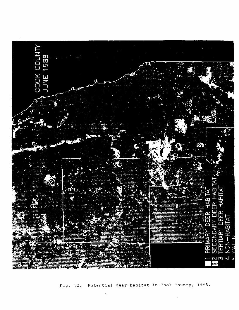
Fia. 12. Potential deer habitat in Cook County, 1988.

U •*°
Fig. 13. Potential deer habitat in DuPage County, 1988.
I

Fig. 14. Potential deer habitat in Kane County, 1988.

Fig. 15. Potential deer habitat in Lake County, 1988.

ACKNOWLEDGEMENTS
Research project W-087-R, Cooperative Forest Wildlife Research, wasconducted with funding from the Federal Aid in Wildlife RestorationAct (Pittman-Robertson)--a cooperative program between the statesand the U.S. Fish and Wildlife Service. The project was sponsoredby the Illinois Department of Conservation. The form, content andinterpretations of data are the responsibility of the IllinoisNatural History Survey, and not of the Illinois Department ofConservation or other cooperating agencies/organizations.