BIOL2300 BiostatisticsChapter 6

Continuous distributions: uniform, normal, exponential

Probability density function• p : R → [0,1] such that

– for all x, 0 ≤ p(x) ≤ 1–

• P( {x: a ≤ x ≤ b}) is definite integral of density function between a and b

Expectation, stdev of continuous r.v. X

Uniform density function

Out[2]=

If A=-1 and B=+1, then uniform density curve is below:

Normal density function

• symmetric about mean µ• Z-score, z = (x-µ)/σ• p(z) = exp(-z2/2) times a constant

Standard normal density

• In standard normal– µ = 0– σ = 1

Out[2]=

Standard normal density function

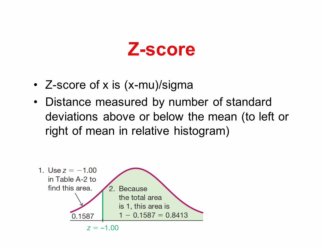
Z-score• Z-score of x is (x-mu)/sigma• Distance measured by number of standard

deviations above or below the mean (to left or right of mean in relative histogram)

Normalizing data

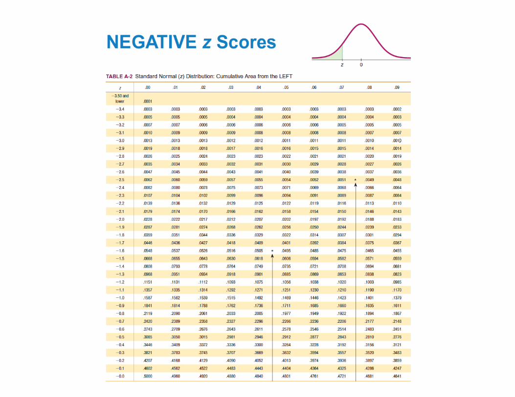
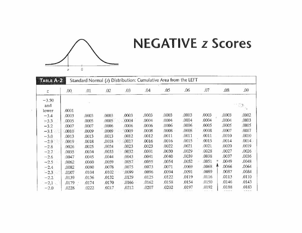
Using Table A-2

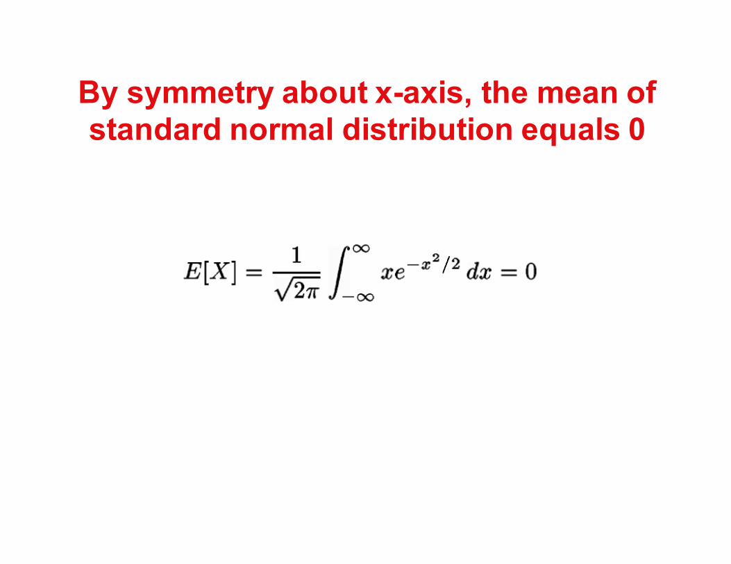
By symmetry about x-axis, the mean of standard normal distribution equals 0

Integration by parts shows variance of standard normal equals 1

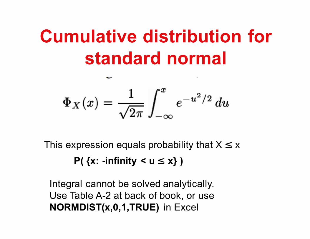
Cumulative distribution for standard normal

Integral cannot be solved analytically.Use Table A-2 at back of book, or useNORMDIST(x,0,1,TRUE) in Excel

This expression equals probability that X ≤ xP( {x: -infinity < u ≤ x} )

Applications of normal distribution

Continuity correction• Continuity correction used when the

continuous normal distribution used to approximate the discrete binomial distribution.

Use Φ to approximate binomial probability in following examples

Suppose p=0.1, n=100, so µ = 10, and σ=sqrt(npq)=3• P(less than 30 successes) = P(k < 30)

• P(more than 30 successes) = P(k > 30)

Use Φ to approximate binomial probability in following examples

Suppose p=0.1, n=100• P(exactly 30 successes) = P(k = 30)

• P(at least 30 successes) = P(k ≥ 30)

• P(at most 30 successes) = P(k ≤ 30)

Comparing cumulative binomial with normal distributions

Comparing binomial with normal distributions (noncumulative)

Superimposition of binomial and normal density graphs

Sampling distribution of the mean

• Sampling distribution of the mean is the distribution of sample means for all samples of size n.

• Sampling distribution of the mean is approximately normal for large sample sizes

CENTRAL LIMIT THEOREM

• The mean of all sample means for samples of size n equals the population mean.– for n=1, this is by definition of population mean– inductively, one can establish the truth for any fixed sample size

Die roll example: sampling WITH replacement, sample size of 2, compute average of sample variances

Die roll example: sampling WITHOUT replacement, sample size of 2, compute average of sample variances

Note: 5.333 =(2+6+8)/3Illustrates that mean of samplesequals population mean.

Sampling distribution of a statistic

• More generally, the sampling distribution of any statistic is the distribution of that statistic over all samples of size n.

• For instance, the sampling distribution of the sample standard deviation (resp. variance) is the distribution of all sample standard deviations (resp. variances) over all samples of size n.

Solution (first for sampling without replacement)

Solution (second, for sampling with replacement)

• For more examples of this form, see my demo python program demoSampleMeansVar.py, in class web pages. See also

• outputDemoSampleMeansVarWithReplacement.txt and

• outputDemoSampleMeansVarWithoutReplacement.txt

Bear age histogram: Mean:43.52, Var: 1116.03StDev:33.41 Max:177 Min:8

Histogram of the means of (X+X+X)/3 for ALL size 3 samples of bear ages: Mean:43.52 Var: 372.01 StDev:19.29Max:177 Min:8. V[(X+X+X)/3] = V[X]/3, so stdev[(X+X+X)/3] =Stdev(X)/sqrt(3). NOTE that bear age stdev (previous slide) divided by sqrt(3), where 3 is sample size, equals 19.29

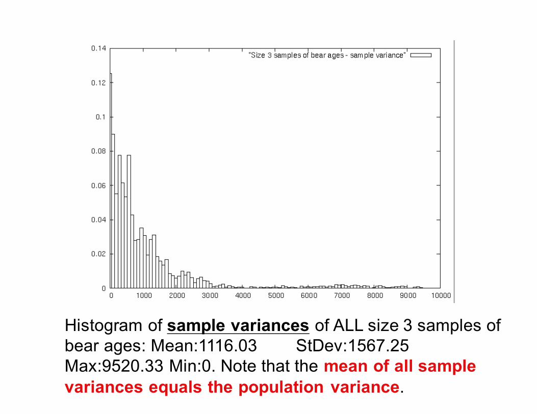
Histogram of sample variances of ALL size 3 samples of bear ages: Mean:1116.03 StDev:1567.25 Max:9520.33 Min:0. Note that the mean of all sample variances equals the population variance.

Histogram of 10,000 repetitions of following experiment:count number of 2’s when rolling die 100 times

Sampling distribution of the proportion

• Sampling distribution of the proportion is the distribution of all sample proportions for all samples of (equal and fixed) size n

• Proportion is number of “successes” over number of “trials” (number of people who plan to vote for candidate X over number of voters, number of red balls over number of balls in urn).

Properties of distribution of sample proportions

• sample proportions tend to target the value of the propulation proportion– relative frequency of r red balls in sample of size n

is P(r/n) = h(n,r;N,R)

• for sufficiently large sample sizes, the distribution of sample proportions approximates a normal distribution (recall that density curve of hypergeometric is approximately normal for sufficiently large sample size.

Unbiased statistic• Unbiased statistic is a statistic that targets the

population parameter

• sample mean, sample variance, sample proportion are unbiased statistics that target population mean, variance and proportion

• median, range, stdev are statistics that do not target corresponding population parameters.

Central Limit Theorem: asymptotically, Z-scores converge to standard normal distribution

Consequences of central limit theorem

• Sampling distribution of the mean (which by definition is the distribution of sample means for all samples of equal and fixed size n) is approximately normal for large sample sizes. The expected value of the sampling distribution for the mean is the population mean.

• Sampling distribution of the proportion is approximately normal for large sample sizes. The expected value of the sampling distribution of the proportion is the population mean.

However ...

• Sampling distribution of the variance is NOT necessarily approximately normal. In fact, we saw that such an example with bear age samples of size 3!

• Nevertheless, the average of the sample variances does equal the population variance, provided that the sampling is done withreplacement.

Mean and stdev of sample means

Mean, variance of sample distribution

• Sampling with replacement (binomial):– Let X be r.v. counting number of successes in sample of size

n, where probability of success is p– E[X] = np, V[X] = npq– Let Y be r.v. counting relative frequency of success in

sample of size n– E[Y] = E[X/n] = np/n = p– V[Y] = V[X/n] =npq/n2 = pq/n = sigma2/n– stdev(Y) = sqrt(pq/n) = sigma/sqrt(n)

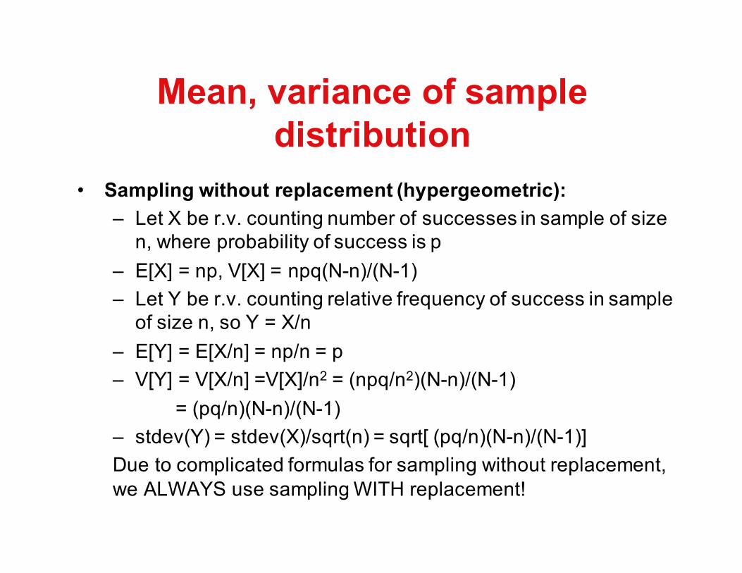
Mean, variance of sample distribution

• Sampling without replacement (hypergeometric):– Let X be r.v. counting number of successes in sample of size

n, where probability of success is p– E[X] = np, V[X] = npq(N-n)/(N-1)– Let Y be r.v. counting relative frequency of success in sample

of size n, so Y = X/n– E[Y] = E[X/n] = np/n = p– V[Y] = V[X/n] =V[X]/n2 = (npq/n2)(N-n)/(N-1)

= (pq/n)(N-n)/(N-1) – stdev(Y) = stdev(X)/sqrt(n) = sqrt[ (pq/n)(N-n)/(N-1)] Due to complicated formulas for sampling without replacement, we ALWAYS use sampling WITH replacement!

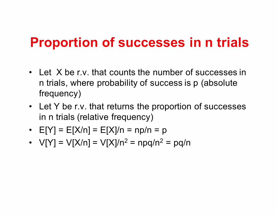
Proportion of successes in n trials

• Let X be r.v. that counts the number of successes in n trials, where probability of success is p (absolute frequency)

• Let Y be r.v. that returns the proportion of successes in n trials (relative frequency)

• E[Y] = E[X/n] = E[X]/n = np/n = p• V[Y] = V[X/n] = V[X]/n2 = npq/n2 = pq/n

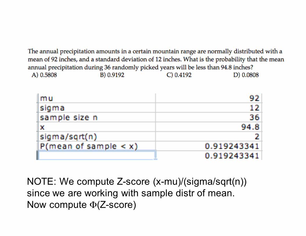
NOTE: We compute Z-score (x-mu)/(sigma/sqrt(n))since we are working with sample distr of mean.Now compute Φ(Z-score)

Simple problems

Probability that an average value satisfies a condition

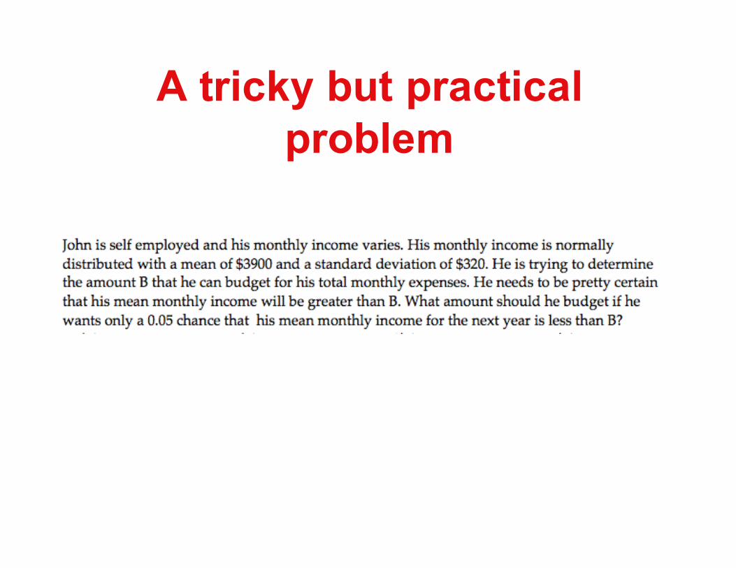
A tricky but practical problem

Solution to John’s budget

A problem solved by previous slides that discussed sampling with and without replacement

Normality test: quantile plot

• sort data in increasing order x1,...,xn

• for each i compute z-scores zi=NORMINV(i/n,0,1), or rather following book zi=NORMINV((2i-1)/2n,0,1)

• determine if scatter plot (xi,zi) is linear

Z-scores

y = 0.0304x - 1.6244

-3

-2

-1

0

1

2

3

1 10 19 28 37 46 55 64 73 82 91 100

Zscores

Linear (Zscores)

Quantile plot for temperatures

Interarrival time, or distance between successive genomic

motifs

What probability distribution is this?

Exponential distribution -continuous analogue of geometric

distribution

Image of exponential distribution for different values of ¸ (called ® in previous

slide)

Excel statistical functions

• average• mode• stdev• stdevp• var• varp• max,min,median

Excel statistical functions• QUARTILE

– Returns the quartile of a data set (quartile = 0,1,2,3,4)

– Syntax: QUARTILE(array,quart)• PERCENTILE

– Returns the k-th percentile of values in a range. For example, you can decide to examine candidates who score above the 90th percentile.

– Syntax: PERCENTILE(array,k)Here k is in interval [0,1] e.g. 0.9.

• STANDARDIZE– Returns Z-score corresponding to x for a distribution with

mean and stdev.– Syntax: STANDARDIZE(x,mean,stdev)

• BINOMDIST– Returns the individual term binomial

distribution probability. – Syntax: BINOMDIST(k,n,p,cumulative).

Used for sampling with replacement

Density function when cumulative = falseCumulative density function when cumulative = true

• HYPGEOMDIST– Returns the probability of a given number of

sample successes, given the sample size, population successes, and population size.

– Syntax: HYPGEOMDIST(r,n,R,N)Used for sampling without replacement

• PERMUT– Returns the number of ORDERED

sequences of length k drawn from a set of size n. Permutations are different from combinations, for which order is not significant.

– Syntax: PERMUT(n,k)

• fact(k)– Returns the factorial k(k-1)(k-2)...1– use permut and fact to compute

combinations

• POISSON– Returns the Poisson distribution. A common

application of the Poisson distribution is predicting the number of events over a specific time, such as the number of cars arriving at a toll plaza in 1 minute.

– Syntax: POISSON(x,mean,cumulative)

• NORMDIST– Returns the normal distribution for the specified mean and

standard deviation. – Syntax: NORMDIST(x,mean,stdev,cumulative)

• NORMDIST– Returns the normal distribution for the specified mean and standard

deviation. – Syntax: NORMDIST(x,mean,stdev,cumulative)

• NORMSINV– Returns the inverse of the standard normal cumulative distribution.

The distribution has a mean of zero and a standard deviation of one.– Syntax: NORMSINV(probability)

Tables from Book