bioinformatics core - purdue

Bioinformatics Core

Jyothi Thimmapuram, Ph.D. [email protected]

Bioinformatics Core Director 1 765-496-6252

RNA-SEQ WORKSHOP, APRIL 2015 – PREREQUISITES

This workshop assumes the user is comfortable operating in the UNIX environment. Without

having a working knowledge of UNIX, it will be very difficult to perform the tasks necessary to

conduct the analysis, and teaching such UNIX skills is beyond the scope of this particular

workshop. Additionally, each participant needs to have a temporary computing account to access

the Hansen cluster, which will be provided upon registration.

EXPERIMENTAL DESIGN

The Sequence Read Archive (SRA) is a database hosted by NCBI that provides a means for

researchers to deposit their primary sequencing data for published studies. One such study, SRA

ID# SRP017778, investigates the transcriptional changes of mouse murine embryonic stem cells

as they differentiate into glutamatergic cortical neurons. This workshop will determine the

differential gene expression (DGE) between two treatments, early neurogenesis sample t7 and

maturing glutamatergic neuron sample t21, with three replicates for each treatment. The analysis

will be limited to the short mouse chromosome 19 to ensure completion in a timely manner.

GETTING STARTED

Login to the Hansen cluster using the provided credentials and PuTTY:

PuTTY is a free program available for

Windows. Use "Host Name"

hansen.rcac.purdue.edu

If using OSX, open terminal and enter:

ssh [email protected]

Today’s Hansen access is temporary and

meant for use with this workshop only

Limited access, free Hansen cluster

accounts are provided upon request –

contact [email protected]

http://www.ncbi.nlm.nih.gov/sra

http://trace.ncbi.nlm.nih.gov/Traces/sra/?study=SRP017778

http://www.chiark.greenend.org.uk/~sgtatham/putty/download.html

mailto:[email protected]

mailto:[email protected]

Bioinformatics Core



DOWNLOADING MATERIALS

After logging into the cluster, the current working directory will be /home/username. Make a new

directory in your scratch space, navigate into that directory, and download the workshop data

pack.

cd $RCAC_SCRATCH // Go to default scratch space

pwd // Display the current directory

< /scratch/hansen/letter/username >

mkdir 2015_RNA-Seq_Workshop // Create a new directory

cd 2015_RNA-Seq_Workshop // Enter the new directory

cp /scratch/hansen/b/bhide/Data.tar.gz . // Copy the package

The file Data.tar.gz is a compressed package containing all necessary files for the workshop.

Unpack and expand the package.

tar –zxvf Data.tar.gz // Decompress and unpack

Now that the files have been downloaded and expanded, enter the same directory as the data.

cd Data // Enter the data directory

Another method of moving/obtaining data is by downloading weblinks through UNIX. Use the

following command to download a copy of this guide.

wget http://web.ics.purdue.edu/~bhide/RNA-Seq2015_Guide.pdf //Download

STEP 1: PREPARING THE DATA

The raw data obtained from a sequencing center will typically be minimally processed and in the

.fastq format. This format preserves the most sequencing information as possible, including

quality scores for each sequenced base. A common .fastq example is as follows:

http://web.ics.purdue.edu/~bhide/RNA-Seq2015_Guide.pdf

Bioinformatics Core



cd Reads

head –n 12 t21rep1_1.fastq // View top few lines of fastq file

@HWI-ST1234:45:C1CELACXX:7:1101:2728:2165/1 1:N:0:GTCCGC //Line 1

CTGGACCAAACACAAACGGTTCCCAGTTTTTTATCTGCACTGCCAAGACTGAATGGCT//Line 2

+ // Line 3

<+1BDBDDD;DBDEE>311+<ADE9EDBEEDI<B?BDDEDI;?BDEDBDB3=@)8=@@// Line 4

Line 1 contains the sequence identifier, which is unique for each read

Line 2 is DNA sequence

Line 3 is usually unused and either has “+” or a repeat of the sequence ID

Line 4 is the Phred quality score in ASCII format, which is often specially formated

depending on the sequencing platform

The first step for any Next Generation Sequencing (NGS) analysis upon receiving data is to

visualize that data before proceeding.

GETTING WORKING SPACE READY

To begin, copy one of the replicates, t21rep1, and the appropriate submission file to the

“Working_space” directory.

cp STEP_1a_Reads_stats.sub Working_space // Copy the sub file

cd Reads // Enter the Reads directory

ls –la // See the available reads files

cp t21rep1_1.fastq ../Working_space // Move the R1 reads

cp t21rep1_2.fastq ../Working_space // Move the R2 reads

pwd // To check whether current directory is Reads

cd ../Working_space // Move into Working_space

ls –la // View directory’s contents

Start by getting a sense of the data metrics - use the following commands to explore the reads.

wc –l t21rep1_* // Count the number of lines in the read files

head –n 12 t21rep1_* // View the first 3 reads of R1 and R2

sed –n ‘2p’ t21rep1_1.fastq | wc –m // Finds the read length

// There are 50 bases, but this command also counts the newline

Bioinformatics Core



CREATING COMPUTING JOBS

Next, use existing software to get quality statistics about the read files. When using

supercomputing clusters, computing tasks are bundled and made into “job” scripts. A central

scheduling program receives the job scripts from anyone with cluster access and runs them when

resources are available. These job scripts are simple text files with a few header lines to specify

cluster resources and the desired UNIX commands to be executed.

All job submission files needed to complete this analysis have already been written and are

labelled STEP_1 through STEP_4. Open STEP_1a and observe how submission files are

formatted.

vi STEP_1a_Reads_stats.sub // Open the job script using ‘vim’

This command will open STEP_1a_Reads_stats.sub for editing. If the file didn’t

already exist, the file will be created and then opened as blank text.

Vim is a powerful text editor with lots of power-user features. Note that mouse input is generally

not supported and the cursor is moved using the arrow keys.

Notice the header lines in the submission file. These lines are preceded by #PBS and pass

arguments to the scheduler.

#PBS –l walltime=4:00:00 // How much time to reserve

#PBS –q bioinf-c // Which queue (subscription) to use

#PBS –l nodes=1:ppn=1 // How many processing cores are needed

*** We have provided access to bioinf-c queue on hansen temporarily for the workshop. For

running your jobs later, you can either use standby queue (for jobs less than 4 hrs) or other

queues on clusters you have access to.

The next line tells the shell where to go after the job starts running. By default all shells start at the

home directory, /home/username. However, usually the files being analyzed will be in the same

directory as the submission file, so the shell needs to change its working directory. The variable

$PBS_O_WORKDIR will always point to the directory from which the job was submitted.

cd $PBS_O_WORKDIR // Go to the job’s working directory

The next several lines specify the software packages that should be available for use during the

job’s computation. Unlike Windows or OSX in which all software is ready to use after installation,

Bioinformatics Core



computing clusters require users to manually specify which software packages (called modules) to

load.

module load bioinfo // Access these modules

module load fastqc // Load the fastqc module

module load fastx // Load the fastx module

More commands related to modules

module avail // Shows all available modules for use

module list // Shows all currently loaded modules

SUBMITTING FIRST JOB – READ STATISTICS

The first job to be submitted will use fastqc to determine read quality statistics information about

the read files has many useful tools, but this step is used for determining base quality statistics and

nucleotide distribution metrics. As with all bioinformatics packages, check the software’s website

for more usage documentation.

fastqc t21rep1_1.fastq

fastqc t21rep1_2.fastq

// Use input reads to determine fastqc

Fastqc for the original files takes longer to run using one core because of memory issue hence we

will use fastx to access quality of the sequences for this workshop.

fastx_quality_stats –Q33 –i t21rep1_1.fastq –o t21rep1_1.stats

// Input the file, calculate phred-33 quality stats, make output

fastq_quality_boxplot_graph.sh -i t21rep1_1.stats -o t21rep1_1.jpg

// Input stats, generate a boxplot, output jpeg image

These commands are done twice, once on the R1 reads and once on the R2 reads. Since no quality

trimming or filtering has been done, the resulting quality statistics graphs will provide a look into

the raw data. To exit the document and submit the job for processing on the super-computer

cluster, use the following commands.

Esc // Exit any mode, such as input mode, in vim

:q! // Quit without saving any changes

http://hannonlab.cshl.edu/fastx_toolkit/commandline.html

Bioinformatics Core



ls –la // View the working directory’s contents

qsub STEP_1a_Reads_stats.sub // Submit the job to the scheduler

< JOB ID.hansen-adm.rcac.purdue.edu >

The resulting output displays the job identification number as well as the cluster that was used for

submission. There are several commands to determine the current status of running jobs, cluster

computer resources, and disk storage space.

qlist // Displays available queue resources

myquota // Displays available storage space

qstat –a –u username // Displays info on currently running jobs

Job ID: The unique numerical identifier given to each submitted job

Username: The owner of the job

Queue: The cluster resource queue being used

Jobname: The name of the submission file

SessID: Assigned after the job starts running by the scheduler

NDS: How many compute nodes are being utilized

TSK: How many total processing cores are being utilized

Req’d Memory: How much memory was reserved for this job

Req’d Time: How much walltime was reserved for this job

S: State of the job, can be:

Q = queued

R = running

C = complete

E = exit

Elap Time: How long the job has been in “Running” status

The best resource to learn more about how to interact with the community clusters can be found in

the RCAC user manuals.

http://www.rcac.purdue.edu/userinfo/userguides.cfm

Bioinformatics Core



A final important note is that finished jobs create two files, an error and an output file. Once these

files are found in the working directory, the job must have been completed or exited due to an

error. Check the *.sub.e* file for error messages, and the *.sub.o* file for any output that

wasn’t saved in a different location.

ASSESSING FIRST JOB COMPLETION

After the first job is complete, the error and output files should be viewed to identify any errors or

concerns.

cat STEP_1a_Reads_stats.sub.eXXXXXXXX // View entire error file

cat STEP_1a_Reads_stats.sub.oXXXXXXXX // View entire output file

Since the commands in Step_1a were meant to generate boxplots and graphs to assess quality of

sequences, check to make sure FastQC results (.html) file exist in the working directory. The

UNIX shell currently being used cannot display images directly. We would transfer FastQC

results file (.html) using SecureFX to your Windows desktop to visualize results file (.html) file

for the workshop.

Other programs are also available called X server for Windows (Xming) which can be installed on

your computer and can be used to transfer images and GUI to user through SSH and visualize

results on Unix/Linux terminal.

TRIMMING THE READS

The reads are ready for trimming now that initial read quality was assessed. Copy the next step to

the working directory, view the working directory’s contents, and explore Step_1b.

cp ../STEP_1b_Reads_trim.sub . // Copy the file to this directory

ls –la // View contents of the working directory

vi STEP_1b_Reads_trim.sub // View the next submission file

Notice that the header information is identical to the previous submission file. This header

information can be reused for similar jobs while just changing the commands. Here a trimming

command is being used instead of the graphical commands of Step_1a.

Bioinformatics Core



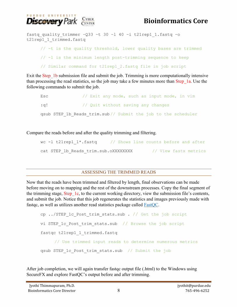
fastq_quality_trimmer –Q33 –t 30 –l 40 –i t21rep1_1.fastq –o

t21rep1_1_trimmed.fastq

// -t is the quality threshold, lower quality bases are trimmed

// -l is the minimum length post-trimming sequence to keep

// Similar command for t21rep1_2.fastq file in job script

Exit the Step_1b submission file and submit the job. Trimming is more computationally intensive

than processing the read statistics, so the job may take a few minutes more than Step_1a. Use the

following commands to submit the job.

Esc // Exit any mode, such as input mode, in vim

:q! // Quit without saving any changes

qsub STEP_1b_Reads_trim.sub // Submit the job to the scheduler

Compare the reads before and after the quality trimming and filtering.

wc -l t21rep1_1*.fastq // Shows line counts before and after

cat STEP_1b_Reads_trim.sub.oXXXXXXXX // View fastx metrics

ASSESSING THE TRIMMED READS

Now that the reads have been trimmed and filtered by length, final observations can be made

before moving on to mapping and the rest of the downstream processes. Copy the final segment of

the trimming stage, Step_1c, to the current working directory, view the submission file’s contents,

and submit the job. Notice that this job regenerates the statistics and images previously made with

fastqc, as well as utilizes another read statistics package called FastQC.

cp ../STEP_1c_Post_trim_stats.sub . // Get the job script

vi STEP_1c_Post_trim_stats.sub // Browse the job script

fastqc t21rep1_1_trimmed.fastq

// Use trimmed input reads to determine numerous metrics

qsub STEP_1c_Post_trim_stats.sub // Submit the job

After job completion, we will again transfer fastqc output file (.html) to the Windows using

SecureFX and explore FastQC’s output before and after trimming.

http://www.bioinformatics.babraham.ac.uk/projects/fastqc/

Bioinformatics Core



STEP 2: MAPPING THE READS

At this stage in the analysis, all of the reads have been preprocessed and are ready to be aligned to

the Mouse reference genome. Such mapping is useful because it describes the genomic location of

each read, from which gene-specific data can be extrapolated (counts, etc).

BUILDING AN INDEXED REFERENCE

The first step when mapping reads is to prepare the genome reference for use. The short read

aligner Tophat requires a multi-fasta reference to be indexed before mapping. Copy Step_2a to the

working directory along with the required fasta file in the reference directory.

cp ../STEP_2a_Index_ref_genome.sub . // Get the script

cp ../References/Mus_chr19.fa . // Copy reference to working

directory

View the job file and notice some differences as compared with Step_1 jobs.

module load bowtie2 // Load Bowtie2 for indexing the ref

bowtie2-build Mus_chr19.fa Mus_chr19 // Create the Mus_chr19

index

qsub STEP_2a_Index_ref_genome.sub //Submit the job

Tophat uses Bowtie2 as its short-read aligner and so, index of reference sequence(s) is also done

using Bowtie2. Indexing a reference creates six additional files:

Mus_chr19.1.bt2

Mus_chr19.2.bt2

Mus_chr19.3.bt2

Mus_chr19.4.bt2

Mus_chr19.rev.1.bt2

Mus_chr19.rev.2.bt2

http://tophat.cbcb.umd.edu/manual.shtml

Bioinformatics Core



MAPPING TO THE REFERENCE

The final mapping step is to align the reads to the indexed genome. This is often the most time

consuming step in an RNA-Seq analysis, but can be greatly expedited by using additional

processing cores. Computational time increases with genome size and number of reads. For this

workshop, we are using a limited number of reads and mapping only to Mouse chromosome 19 to

ensure timely completion.

Copy the Step_2b submission file to the working directory, observe its contents, and submit the

job. After several minutes, the job will finish and produce several new files.

cp ../STEP_2b_Map_ref.sub . // Get the job script

qsub STEP_2b_Map_ref.sub // Submit the job

vi STEP_2b_Map_ref.sub // Look through job script for some

additional commands

If we add few lines in beginning and end of any of job scripts, it will print the start time (display

time when job started) and end time (display time when job finished) and calculates total time

taken for job to complete. Such commands might be useful to know total time required to run job,

especially if you are running time consuming jobs like mapping reads to reference genome,

genome assembly etc.

starts=$(date +"%s") # %s saves time in seconds and

current date which is saved in starts variable

start=$(date +"%r, %m-%d-%Y") #%r 12-hour time, %m - month, %d

day of month and %Y - year.

ends=$(date +"%s")

end=$(date +"%r, %m-%d-%Y")

diff=$(($ends-$starts))

#diff variable saves difference between starts and ends values

hours=$(($diff / 3600)) #hours variable

dif=$(($diff % 3600)) #dif variable

minutes=$(($dif / 60)) #minutes variable

seconds=$(($dif % 60)) #seconds variable

cat STEP_2b_Map_ref.sub.eXXXXXX // View run messages

cd tophat_out // This is the standard output directory for

tophat

mv accepted_hits.bam t21rep1.bam // Rename the mapping file

mv t21rep1.bam ../ // Relocate the mapping file

Bioinformatics Core



A good way to view mapping statistics from tophat runs is to check the mapping logs. From

within the \tophat_out directory, navigate to the logs sub-directory and browse metrics for the R1

(left) and R2 (right) reads.

cd logs // Enter the logs sub-directory

ls –la // See all of the various log files created

cat bowtie.left_kept_reads.log // Check the R1 mapping metrics

cat bowtie.right_kept_reads.log // Check the R2 mapping metrics

Example metrics:

754050 reads; of these:

754050 (100.00%) were unpaired; of these: o 215516 (28.58%) aligned 0 times

o 486843 (64.56%) aligned exactly 1 time

o 51691 (6.86%) aligned >1 times

71.42% overall alignment rate

cd ../ // Go back to the ‘tophat_out’ directory

// Look for ‘align_summary.txt’ to get an idea of alignment

statistics of paired reads

cd ../ // Go back to the ‘Working_space’ directory

STEP 3: USING CUFFLINKS TO IDENTIFY DGE

Cufflinks is a popular software package that uses Tophat output to assemble transcripts and

estimate transcript abundance. Cufflinks can be used to find de novo transcripts or read in known

transcripts from a reference .gtf file. Copy the Step_3a submission file into the working directory,

browse the job script, and submit.

cp ../References/Mus_chr19.gtf . // Get reference gtf file

cp ../STEP_3a_Cufflinks.sub . // Get the job script

cufflinks -G Mus_chr19.gtf t21rep1.bam

// View command in job script -G mode uses known genes only

qsub STEP_3a_Cufflinks.sub // Submit the job

http://cufflinks.cbcb.umd.edu/manual.html

Bioinformatics Core



After the job is complete, check the error and output files to be sure there were no problems. The

file of interest that was created by this step is called transcripts.gtf.

cat STEP_3a_Cufflinks.sub.* // View both error and output at once

head –n 20 transcripts.gtf // See the cufflinks output

mv transcripts.gtf t21rep1.gtf // Rename the output as the

sample ID

Every step in the NGS analysis process needs to be done on all 6 replicates to create 6 different

cufflinks output .gtf files. Through this guide, a single replicate, t21rep1, has been completed. To

save time, copy the previously finished output for the remaining 5 sample into the working

directory.

cp ../Completed_files/STEP_3_supplementary_files/* .

// Copy .gtf files to ‘Working_space’ directory

MERGING CUFFLINKS OUTPUT WITH CUFFMERGE

The next step of the cufflinks pipeline is to use cuffmerge to combine annotation files. This is

necessary for comparing transcripts between samples. Copy Step_3b to the working directory, but

wait to submit, as some preparation is necessary. See the submission file:

cp ../STEP_3b_Cuffmerge.sub . // Get the job script

cuffmerge -g Mus_chr19.gtf assembly_list.txt

< assembly_list.txt is a text file that needs to be made >

ls | grep -Po "t.+rep..gtf" > assembly_list.txt

cat assembly_list.txt // See the necessary formatting of this file

// This file tells cuffmerge which .gtfs to use for analysis

Now that the assembly_list.txt file has been created, submit the job and browse the resulting files.

qsub STEP_3b_Cuffmerge.sub // Submit the job

ls –lta // List directory contents in order of creation

cd merged_asm // Enter the cuffmerge directory

head –n 15 merged.gtf // Browse the combined .gtf file

http://cufflinks.cbcb.umd.edu/manual.html#cufflinks

Bioinformatics Core



mv merged.gtf ../ // Move merged.gtf into the working

directory

cd ../ // Return to the working directory

QUANTIFYING GENE/TRANSCRIPT EXPRESSION USING CUFFQUANT

Cuffquant computes gene and transcript expression profiles and saves these profiles such that it

can be analyzed in a timely manner by Cuffdiff (last step to determine DGE). Cuffquant reduces

the computational load of quantifying gene and transcript expression especially if there are more

than a handful of libraries. Cuffquant is able to take the .bam mapping files made from each of the

6 samples along with the merged.gtf file and generate .cxb (compressed binary file). Copy the

Step_3c submission file to the working directory.

cp ../STEP_3c_Cuffquant.sub . // Get the job script

cuffquant -o ./t21rep1_cfquant merged.gtf t21rep1.bam

// View the cuffquant command in job script

qsub STEP_3c_Cuffquant.sub // Submit the job

After cuffquant job is finished, let us check the output files generated in t21rep1_cfquant folder.

cd t21rep1_cfquant // Enter cuffquant output directory

mv abundances.cxb ../t21rep1.cxb

// Rename .cxb file and move to ‘Working_space’ directory

IDENTIFYING DGE USING CUFFDIFF

Cuffdiff is the last step of the three part cufflinks/cuffmerge/cuffdiff pipeline for determining

DGE. Cuffdiff is able to take the .cxb files made from each of the 6 samples using cuffquant along

with the merged.gtf file to locate and statistically compare genes. Copy the Step_3d submission

file to the working directory, as well as the mapping files for the other 5 samples.

cp ../STEP_3d_Cuffdiff.sub . // Get the job script

cp ../Completed_files/STEP_3_complete/cuffquant/t21rep2.cxb .

cp ../Completed_files/STEP_3_complete/cuffquant/t21rep3.cxb .

cp ../Completed_files/STEP_3_complete/cuffquant/t7rep*.cxb .

< View the cuffdiff command in the job script >

http://cufflinks.cbcb.umd.edu/manual.html#cufflinks

Bioinformatics Core



cuffdiff -v merged.gtf -L t7,t21 t7rep1.cxb,t7rep2.cxb,t7rep3.cxb

t21rep1.cxb,t21rep2.cxb,t21rep3.cxb

// -v specifies the cuffmerge output file

// -L gives text labels to the treatments being compared

// The final list of .cxb files generated by Cuffquant:

// Within a treatment, replicates are separated by commas

// Treatment groups are separated by a space

To stay organized, make a new directory for running cuffdiff and place all necessary files inside

and run the job script.

mkdir cuffdiff_analysis // Create the directory

mv merged.gtf cuffdiff_analysis // Move the annotation file

mv *.cxb cuffdiff_analysis // Move all mapping files

mv STEP_3d_Cuffdiff.sub cuffdiff_analysis

// Move the submission file

Enter the directory and submit the job.

cd cuffdiff_analysis // Enter the cuffdiff directory

qsub STEP_3d_Cuffdiff.sub // Submit the job

UNDERSTANDING THE CUFFDIFF OUTPUT

Cuffdiff creates numerous files containing information regarding alternative splice junctions,

novel transcripts, etc. The file containing DGE information pertaining to known transcripts is

called gene_exp.diff. Browse this file to examine the RNA-Seq analysis results using the

following table.

Column Column name Example Description

1-2 Tested id / gene id

XLOC_000001 A unique identifier describing the transcipt, gene, primary transcript, or CDS being tested

3 gene Lypla1 The gene_name(s) or gene_id(s) being tested

Bioinformatics Core



4 locus chr1:4797771-4835363

Genomic coordinates for easy browsing to the genes or transcripts being tested.

5 sample 1 Liver Label (or number if no labels provided) of the first sample being tested

6 sample 2 Brain Label (or number if no labels provided) of the second sample being tested

7 Test status NOTEST Can be one of OK (test successful), NOTEST (not enough alignments for testing), LOWDATA (too complex or shallowly sequenced), HIDATA (too many fragments in locus), or FAIL, when an ill-conditioned covariance matrix or other numerical exception prevents testing.

8 FPKMx 8.01089 FPKM of the gene in sample x

9 FPKMy 8.551545 FPKM of the gene in sample y

10 log2(y/x) 0.06531 The (base 2) log of the fold change y/x

11 test stat 0.860902 The value of the test statistic used to compute significance of the observed change in FPKM

12 p value 0.389292 The uncorrected p-value of the test statistic

13 q value 0.985216 The FDR-adjusted p-value of the test statistic

14 significant no Can be either "yes" or "no", depending on whether p is greater then the FDR after Benjamini-Hochberg correction for multiple-testing

STEP 4: MAKING THE COUNTS MATRIX

The previous mapping step resulted in a file, t21rep1.bam, which contains positions for aligning

each read onto the genome. Another reference file, Mus_chr19.gtf, contains positions defining

where each gene is located in the genome. By intersecting these two files it is possible to

determine which reads are mapping to particular genes. The number of reads mapping to a certain

gene are scored as ‘counts’ and used for downstream differential gene expression (DGE) analysis.

Annotation files (.gtf/.gff/.gff3) are tab-delimited text documents with specific formatting to

describe where certain features are located in a reference genome. See the Ensembl explanation of

this file type for more details.

Copy the Step_4 submission file to the working directory. Additionally, the Mouse .gtf file will

need to be copied to the working directory from the /References directory. Browse the job script

and see the commands used to make a counts file. Aggregating counts uses the HTSeq package.

cp ../STEP_4_Make_counts_matrix.sub . // Get the job script

cp ../References/Mus_chr19.gtf . // Get the .gtf file

vi STEP_4_Make_counts_matrix.sub // Open job script to have

a look at it

samtools sort -n t21rep1.bam t21rep1_sorted

// Sort the .bam file

samtools view t21rep1_sorted.bam > t21rep1.sam

// Convert to .sam file

http://useast.ensembl.org/info/website/upload/gff.html

http://www-huber.embl.de/users/anders/HTSeq/doc/count.html#count

Bioinformatics Core



htseq-count -q -m union -s no -t exon -i gene_id t21rep1.sam

Mus_chr19.gtf > t21rep1.counts

// Follow the HTSeq link for an explanation of all

parameters

qsub STEP_4_Make_counts_matrix.sub // Submit the job

VIEWING THE COUNTS MATRIX

After the HTSeq job finishes there will be a single column of counts representing every gene in

Mouse chromosome 19. Each row is named after the gene ID as found in the Mus_chr19.gtf file,

and will be present even if no counts were found (which is very helpful for comparing between

samples).

head –n 30 t21rep1.counts // Observe the how the counts are

stored

tail –n 10 t21rep1.counts // See why counts were lost

no_feature 160506 // Aligned in non-gene region ambiguous 17416 // Aligned in region with 2 genes too_low_aQual 0 // Quality is too poor not_aligned 0 // No alignment found alignment_not_unique 616529 // Aligned to many places

The purpose of a counts matrix is to see changes across treatments for particular genes. Thus far,

counts were only generated for a single replicate of a single treatment (1 out of 6 different

samples). To generate the full counts matrix, copy the previously completed *.counts files into

the working directory and execute the following commands.

cp ../Completed_files/STEP_4_complete/t21rep2.counts .

// Copy to here

cp ../Completed_files/STEP_4_complete/t21rep3.counts .

// Copy to here

cp ../Completed_files/STEP_4_complete/t7rep*.counts .

// Copy to here

Bioinformatics Core



< The following commands generate the combined matrix >

echo -e "Genes\tt7r1\tt7r2\tt7r3\tt21r1\tt21r2\tt21r3" >

matrix.part1

paste t7rep*.counts t21rep*.counts > matrix.part2

cut -f 1,2,4,6,8,10,12 matrix.part2 > matrix.part3

cat matrix.part1 matrix.part3 > counts_matrix.txt

< The complete matrix is counts_matrix.txt >

head counts_matrix.txt // View the top of the matrix

wc –l counts_matrix.txt

// Count number of lines in file.971 lines are present

sed ‘967,971d’ < counts_matrix.txt > counts_matrix_final.txt

// Remove last 5 lines of HTSeq statistics information from

the file

Notice the trends between the samples – the counts in the t7 replicates group apart from the t21

replicates. Similarly, certain genes have no expression in any of the replicates. This matrix can

now be processed by a variety of statistical analysis tools for determining DGE, such as the

commonly used R packages edgeR, DESeq2, or limma. Instead of venturing into R for this

workshop, we determined DGE analysis using Cufflinks suite of programs.

http://www.r-project.org/

http://www.bioconductor.org/packages/release/bioc/html/edgeR.html

http://bioconductor.org/packages/release/bioc/html/DESeq.html

http://www.bioconductor.org/packages/release/bioc/html/limma.html

bioinformatics core - purdue

Documents