bioinformatic analyses in microsatellite-based … · v i bioinformatic analyses in...
TRANSCRIPT

v i
BIOINFORMATIC ANALYSES IN MICROSATELLITE-BASED
GENETIC DIVERSITY OF TURKISH SHEEP BREEDS
A THESIS SUBMITTED TO
THE GRADUATE SCHOOL OF INFORMATICS
OF
MIDDLE EAST TECHNICAL UNIVERSITY
BY
HANDE ACAR
IN PARTIAL FULFILLMENT OF THE REQUIREMENTS FOR THE DEGREE OF
MASTER OF SCIENCE
IN
BIOINFORMATICS
SEPTEMBER 2010

ii
Approval of the Graduate School of Informatics
___________________________
Prof. Dr. Nazife BAYKAL
Director
I certify that this thesis satisfies all the requirements as a thesis for the degree of
Master of Science.
___________________________
Prof. Dr. Nazife BAYKAL
Head of Department
This is to certify that I have read this thesis and that in my opinion it is fully
adequate, in scope and quality, as a thesis for the degree of Master of Science.
__________________
Prof. Dr.Ġnci TOGAN
Supervisor
Examining Committee Members
Assist. Prof. Dr. YeĢim AYDIN SON (METU, II) _______________________
Prof. Dr. Ġnci TOGAN (METU, BIOL)_____________________
Assist. Prof. Dr. Tolga CAN (METU, CENG)____________________
Assoc. Prof. Dr. Ġrfan KANDEMĠR (Ankara Uni) ______________________
Dr. Evren KOBAN (TUBITAK, MAM)_________________

iii
I hereby declare that all information in this document has been obtained and
presented in accordance with academic rules and ethical conduct. I also declare
that, as required by these rules and conduct, I have fully cited and referenced
all material and results that are not original to this work.
Name, Last Name: Hande Acar
Signature:

iv
ABSTRACT
BIOINFORMATIC ANALYSES IN MICROSATELLITE-BASED
GENETIC DIVERSITY OF TURKISH SHEEP BREEDS
Acar, Hande
M.Sc. Department of Bioinformatics
Supervisor: Prof. Dr. Ġnci Togan
September 2010, 129 pages
In the present study, within and among breed genetic diversity in thirteen Turkish
sheep breeds (Sakız, Karagül, HemĢin, Çine Çaparı, Norduz, Herik, Akkaraman,
Dağlıç, Gökçeada, Ġvesi, Karayaka, Kıvırcık and Morkaraman; in total represented
by 628 individuals) were analyzed based on 20 microsatellite loci.
Loci were amplified by Polymerase Chain Reactions and products were
electronically recorded and converted into [628 x 20] matrix representing genotypes
of individuals. Reliability of the genotyping and genetic diversity analyses were done
by means of various bioinformatics tools. For the analyses, various statistical
methods (Fisher‟s Exact Test, Neighbor-Joining tree construction, Factorial
Correspondence Analysis (FCA), Analysis of Molecular Variation, Structure
Analysis and Delaunay Analysis) were used. Since, inputs of some software were not
compatible with the outputs of other software some Java classes were written
whenever necessary.

v
Analyses revealed that among the major breeds Dağlıç, Karayaka and Morkaraman
breeds are highly admixed but Kıvırcık, Akkaraman and Ġvesi are relatively distinct.
Among the minor breeds, distinctness of Hemsin, Sakız, Çine Çaparı, Gökçeada and
Karagül are more pronounced compared to all of the examined breeds. Since highly
admixed individuals can be identified by Structure and FCA tests, results of the
present study, which is part of a national project with the acronym TURKHAYGEN-
I (www.turkhaygen.gov.tr), were found to be promising in establishing and
managing relatively pure conservation flocks for the Turkish native sheep breeds
which are believed to be the reservoirs of genetic variability.
Keywords: Bioinformatics, Turkish sheep breeds, microsatellites, genetic diversity,
conservation

vi
ÖZ
TÜRK KOYUN IRKLARININ GENETĠK ÇEġĠTLĠLĠKLERĠNĠN
MĠKROSATELĠT BELĠRTEÇLER KULLANILARAK
BĠYOENFORMATĠK YÖNTEMLERLE ĠNCELENMESĠ
Acar, Hande
Yüksek Lisans, Biyoenformatik Bölümü
Tez Yöneticisi: Prof. Dr. Ġnci Togan
Eylül 2010, 129 Sayfa
Bu çalıĢmada, on üç Türk koyun ırkının (Sakız, Karagül, HemĢin, Çine Çaparı,
Norduz, Herik, Akkaraman, Dağlıç, Gökçeada, Ġvesi, Karayaka, Kıvırcık ve
Morkaraman; toplamda 628 birey) ırk içi ve ırklar arası genetik çeĢitliliği, 20
mikrosatelit lokusu kullanılarak incelenmiĢtir.

vii
Lokuslar Polimeraz Zincir Reaksiyonu kullanılarak yükseltgenmiĢ ve ürünler
elektronik ortamda kaydedilip bireylerin genotiplerini temsil eden [628 x 20]‟lik bir
matrise çevrilmiĢtir. Genotiplemenin güvenilirliği ve genetik çeĢitlilik analizi pek
çok biyoenformatik araçları kullanılarak gerçekleĢtirilmiĢtir. Analizler için Fischer‟ın
Kesinlik Testi, KomĢu-BirleĢtirme Ağaçları, Faktöriyel BirleĢtirici Analizi (FCA),
Moleküler Varyasyon Analizi, Yapı Analizi ve Delaunay Analizi gibi istatistiksel
yöntemler kullanılmıĢtır. Bu analizler yapılırken bazen bir yazılımın çıktısı diğer
yazılımın girdisi ile uyumlu olmadığından gerek görülen durumlarda çevirimi
yapacak Java Sınıfları geliĢtirilmiĢtir.
GerçekleĢtirilen analizler temel büyük ırklardan Dağlıç, Karayaka ve Morkaraman
ırklarının yüksek derecede karıĢmıĢ olduklarını; ancak Kıvırcık, Akkaraman ve Ġvesi
ırklarının göreceli olarak bu ırklardan ayrılmıĢ olduğunu göstermiĢtir. Diğer taraftan
küçük ırklardan HemĢin, Sakız, Çine Çaparı, Gökçeada ve Karagül ırklarının
farklıkları diğerlerine gore daha çok göze çarpmaktadır. Yapı ve FCA testleri ile
yüksek derecede karıĢmıĢ bireyler saptanabildiğinden, TURKHAYGEN-I
(www.turkhaygen.gov.tr) ulusal projesinin de bir parçası olan bu çalıĢmanın
sonuçları, zor çevresel koĢullara uyum sağlayabilen genetik çeĢitliliğin korunmuĢ
olduğu düĢünülen Türk yerli koyun ırkları için oldukça saf koruma sürüleri
oluĢturmada umut vericidir.
Anahtar Kelimeler: Biyoenformatik, Türk koyun ırkları, mikrosatelit, genetik
çeĢitlilik, koruma

viii
To my mother…

ix
ACKNOWLEDGMENTS
It is a pleasure to thank the many people who made this thesis possible.
It is difficult to overstate my gratitude to my supervisor and my mentor, Prof. Dr.
Ġnci Togan. Throughout the last four years, she provided guidance in all aspects of
my life, encouragement, sound advice, good teaching. I would have been lost without
her. Moreover, I will never forget the days I had in Burhaniye with her family.
I would like to thank the many people who have taught me all the skills in the
laboratory and in the field with their graciousness and friendship: Dr. Havva Dinç,
Dr. Evren Koban, Assist. Prof. Emel Özkan, ġ. Anıl Doğan, Eren Yüncü. Also
special thanks to Lab147 Team for their support and for providing a stimulating and
fun environment: N. DilĢad DağtaĢ (countless number of gels...), Ġ. Cihan Ayanoğlu
(who dared to be my student in an undergraduate project), Sevgin Demirci, Begüm
Uzun, Arzu Karahan (those fishes do not have DNA, they are from space).
Throughout the whole masters marathon, my dear friend H. Alper Döm was always
with me, supporting me, helping me, working with me till morning… I cannot thank
enough to you.
Throughout the last six years, they would be impossible without you, Tuğba Keskin,
my best friend, was with me all the time. Thank you my dear for helping me to find
strength to get through the difficult times, and for all the emotional support,
camaraderie, entertainment, and caring. I love you…

x
He has made available his support in a number of ways; I want to express my
gratefulness to Yıldıray Kabak for being with me in all circumstances. I know that
you deserve a dedication of this thesis because of your contributions, and you have it
here.
Lastly, and most importantly, I wish to thank my family, my mother Asuman Acar,
to whom I dedicate this thesis, she is like a source of strength and morale in my
desperate moments; my sisters Handan Acar, you were more than a sister for me,
more than a friend, more than many things… and Aydan Acar, she never unclasp my
hand. They supported me, raised me, taught me, and loved me...
This study was supported by The Scientific and Technical Research Council of
Turkey (TUBITAK) as a part of the project In Vitro Conservation and Preliminary
Molecular Identification of Some Turkish Domestic Animal Genetic Resources-I
(TURKHAYGEN-I) under the grant number 106G115. Also, I gratefully
acknowledge the fellowship I had through my master years from The Scientific and
Technical Research Council of Turkey (TUBITAK) - BĠDEB.

xi
TABLE OF CONTENTS
ABSTRACT ................................................................................................................ iv
ÖZ ............................................................................................................................... vi
DEDICATION ……………………………………………………………………. viii
ACKNOWLEDGMENTS …………………………………………………………..ix
TABLE OF CONTENTS ............................................................................................ xi
LIST OF TABLES ..................................................................................................... xv
LIST OF FIGURES .................................................................................................. xvi
LIST OF ABBREVIATIONS .................................................................................. xvii
CHAPTER
1 INTRODUCTION ............................................................................................... 1
1.1 Part of Anatolia as the center of domestication for many livestock species . 1
1.2 Conservation Studies for Turkish Sheep Breeds ........................................... 5
1.3 Microsatellites and Bioinformatics Analysis in Relation to
Genetic Diversity Analyses ...................................................................................... 7
1.4 Justification and objectives of the study ..................................................... 10
2 MATERIALS AND METHODS ....................................................................... 12
2.1 Samples, Breeds and Sampling ................................................................... 12
2.2 Laboratory Experiments .............................................................................. 16
2.2.1 DNA Isolation from Blood .................................................................. 16
2.2.2 Adjustment of DNA Concentration by Agarose Gel Electrophoresis . 17
2.2.3 Microsatellites ...................................................................................... 18

xii
2.2.4 Polymerase Chain Reaction (PCR) Conditions ................................... 18
2.3 Data Analysis .............................................................................................. 22
2.3.1 Reliability of the Microsatellite Data ................................................... 22
2.3.2 Methods used for the Statistical Analyses ........................................... 24
2.3.2.1 Estimation of Genetic Variation ................................................... 24
2.3.2.1.1 Allelic variation .......................................................................... 24
2.3.2.1.1.1 Allelic Richness ................................................................... 24
2.3.2.1.1.2 Polymorphic Information Content (PIC) ............................. 25
2.3.2.1.1.3 Private alleles ....................................................................... 25
2.3.2.1.2 Heterozygosity ............................................................................ 26
2.3.2.2 F-statistics: FIS and Pairwise FST Values ...................................... 26
2.3.2.3 Genetic Distance Estimations and Phylogenetic Tree
Construction ................................................................................................... 28
2.3.2.3.1 Cavalli-Sforza and Edwards‟ Chord Distance, DC ..................... 29
2.3.2.3.2 Nei's DA Genetic Distance ......................................................... 29
2.3.2.3.3 Neighbor Joining (NJ) Tree ........................................................ 30
2.3.2.4 Analysis of Molecular Variance (AMOVA) ................................ 31
2.3.2.5 Factorial Correspondence Analysis (FCA) ................................... 34
2.3.2.6 Structure Analysis ......................................................................... 34
2.3.2.7 Delaunay Network Analysis ......................................................... 36
3 RESULTS .......................................................................................................... 37
3.1 Results of the Laboratory Experiments ...................................................... 37
3.1.1 Extracted DNA and Results of Polymerase Chain Reaction (PCR) ...... 37
3.1.2 Microsatellite Analyses .......................................................................... 39

xiii
3.2 Statistical Analyses .................................................................................... 40
3.2.1 Reliability of the Microsatellite Data ..................................................... 40
3.2.2 Breed Based Analyses ............................................................................ 44
3.2.2.1 Genetic Variation Analyses .......................................................... 44
3.2.2.1.1 Allelic Variation ......................................................................... 44
3.2.2.1.1.1 Allelic Richness ................................................................... 45
3.2.2.1.1.2 Polymorphism Information Content (PIC) ........................... 47
3.2.2.1.1.3 Private Alleles ...................................................................... 48
3.2.2.1.2 Heterozygosity Analysis ............................................................. 49
3.2.2.2 F-Statistics .................................................................................... 51
3.2.2.2.1 FIS Values ................................................................................... 51
3.2.2.2.2 Pairwise FST Values .................................................................... 52
3.2.2.3 Genetic Distance Estimations and Phylogenetic Tree
Construction ................................................................................................... 54
3.2.2.3.1 Cavalli-Sforza and Edwards‟ Chord Distance, DC ..................... 54
3.2.2.3.2 Nei's DA Genetic Distance .......................................................... 54
3.2.2.3.3 Neighbor Joining (NJ) Tree Construction: Based on
“Cavalli-Sforza and Edwards‟ Chord Distance, DC” and “Nei's DA Genetic
Distance” .................................................................................................... 56
3.2.2.4 Analysis of Molecular Variance (AMOVA) ................................ 59
3.2.3 „Individuals within Populations‟ Based Analyses ................................. 65
3.2.3.1 Factorial Correspondence Analysis (FCA) ................................... 65
3.2.3.2 Structure ........................................................................................ 67
3.2.4 Genetic Barrier Estimation: Delaunay Network Analysis ..................... 71

xiv
4 DISCUSSION .................................................................................................... 73
4.1 Interdisciplinary nature of the study; analyses and their complementary
contributions to the understanding of data. ............................................................ 73
4.2 Revisiting the results of the present study ................................................. 75
4.3 Comparative evaluation of the results with those of the previous studies . 80
4.4 Recommendations in relation to genotypng based on microsatellite loci .. 83
4.5 Possible implementations of the results ..................................................... 87
5 CONCLUSION .................................................................................................. 91
REFERENCES .......................................................................................................... 93
APPENDICES ......................................................................................................... 104
A ................................................................................................................... 104
B ................................................................................................................... 105
C ................................................................................................................... 107
D ................................................................................................................... 111
E ................................................................................................................... 117

xv
LIST OF TABLES
Table 2-1 Description of the samples ........................................................................ 13
Table 2-2 Studied sheep microsatellite DNA markers............................................... 19
Table 2-3 Microsatellite groups. ................................................................................ 20
Table 2-4 Constituents of the PCR mixture. .............................................................. 20
Table 2-5 PCR amplification protocol for group I loci .............................................. 21
Table 2-6 General AMOVA table ............................................................................. 32
Table 3-1 Comparative representation of allele numbers .......................................... 41
Table 3-2 Null allele frequencies of thirteen breeds for 20 microsatellite loci......... 42
Table 3-3 P-value for genotypic disequilibrium of 19 microsatellite loci ............... 43
Table 3-4 Allelic richness table. .............................................................................. 46
Table 3-5 PIC of each locus and breed. .................................................................... 47
Table 3-6 The distribution of private alleles and their frequencies. ........................ 48
Table 3-7 Epected heterozygosities and deviations from H-W equilibrium ............ 50
Table 3-8 FIS values for each breed based on 19 loci ................................................ 51
Table 3-9 Pairwise comparison matrix of FST values with and without ENA
corrections. ................................................................................................................. 53
Table 3-10 Pairwise Cavalli-Sforza and Edwards‟ chord distance, DC , and pairwise
Nei‟s DA genetic distance values with ENA corrections between thirteen breeds. ... 55

xvi
LIST OF FIGURES
Figure 1-1 Three main livestock domestication centers on a world map. ................... 2
Figure 1-2 Domestication sites of sheep, pig, cattle and goats in Fertile Crescent. ... 3
Figure 2-1 . The distribution of sites for the collected sheep breeds in Turkey ........ 12
Figure 3-1 DNA bands before adjustment of concentrations of the DNAs. ............. 37
Figure 3-2 DNA bands after adjustment of concentrations of the DNAs. ................ 38
Figure 3-4 Microsatellite electropherogram representing three loci ......................... 39
Figure 3-5 NJ tree with Cavalli-Sforza DC distance ................................................. 56
Figure 3-6 NJ tree with DA distance, data with ENA corrections ............................. 57
Figure 3-7 NJ tree with DA distance.. ....................................................................... 58
Figure 3-8 FCA result showing the relationship between all of the individuals
analyzed in the study.. ................................................................................................ 66
Figure 3-9 The graph of the second order rate of change of the likelihood function
(ΔK = m|L‟‟(K)|/ s[L(K)]) with respect to K. ............................................................ 67
Figure 3-10 Structure Bar Plot at K=10 .................................................................... 68
Figure 3-11 Structure Bar Plot at K=2. ..................................................................... 70
Figure 3-12 Delaunay Network by using Cavalli-Sforza and Edwards‟ chord
distance, DC values. .................................................................................................... 71
Figure 3-13 Delaunay Network by using Nei's DA genetic distance with ENA
corrections values.. ..................................................................................................... 72
Figure 4-1 STRUCTURE Analyses for the Breeds from Northern Eurasia ........... 83

xvii
LIST OF ABBREVIATIONS
°C : Degrees Celsius
μL : Microliter
AMOVA: Analysis of Molecular Variance
APS: Ammonium Per Sulfate
Arlequin: An Integrated Software Package for Population Genetics Data
Analysis
bp : Base Pair
BP: Before Present
BSA: Bovine Serum Albumine
dNTP: Deoxynucleotide Triphosphate
dH2O : Distilled Water
DNA : Deoxyribonucleic Acid
EDTA : Ethylene Diamine Tetra Acetic Acid
e.g: For example
EtBr: Ethidium Bromide
K3EDTA: Potassium EDTA
M: Molar
MEGA : Molecular Evolutionary Genetics Analysis
mg: Miligram
MgCl2 : Magnesium Chloride
MARA: Ministry of Agriculture and Rural Affairs
mL: Milliliter
mM: Millimolar
mtDNA : Mitochondrial DNA
NaAc: Sodium Acetate
ng: Nanogram
NJ: Neighbor Joining
PCR: Polymerase Chain Reaction
pH : Potential of Hydrogen
PHYLIP: Phylogeny Inference Package Software
pmol: Picomoles
rpm : Rotations per Minute
RT: Room Temperature
SDS: Sodium Dodecyl Sulfate

xviii
Taq : Thermus aquaticus
TBE: Tris Borate EDTA
TEMED: Tetramethylethylenediamine
UV: Ultra Violet
V: Volt

1
CHAPTER 1
INTRODUCTION
1.1 Part of Anatolia as the center of domestication for many livestock species
Nearly 12000 years before present (BP) first by the cultivating the plants and then by
taming and domesticating the animals, the life style of human beings have changed
from “hunting- gathering” to “farming-herding” (Naderi, et al. 2008). This transition
marked the Neolithic age. Domestication of animals provided many advantages to
human beings, for instance, they had steady food supply (meat, eggs, milk), they
received protection and companionship by dogs (yet it must be remembered that
domestication of dog was before the Neolithic age during the time of hunting), they
had clothing (with materials like wool and hides) and could make use of the animal
power in plowing, carrying heavy loads.
Studies to unravel the place(s) of this transition as well as phases of the transition
have been carried out for many decades, but still largely unknown. Previously
answers to those questions were important mainly from the anthropological point of
view and the researches were performed mainly by archeologists. Results were
constrained by the data from those archeological sites where remains were unearthed.
Until the late 90‟s, morphological changes were considered as the sign of transition
from the wild animals to domesticated ones, such as sharp decrease in the size of
animals (Zeder, 2006). However, as the information from new sites were gathered,
and with the new realizations it was accepted that domestication might have started
before the occurrence of animal size change. In flock, the old female to young female
ratio should increase in the managed flock, because, in the managed flock, higher
numbers of females giving milk and giving birth to young were kept longer. Also,
few males were necessary to continue the flock; hence female to male ratio should

2
also increase. These changes in ratios when observed by archeozoologists are now
accepted as the sign of early domestication at the archeological sites (Zeder, 2008).
Figure 1-1 Three main livestock domestication centers on a world map, taken from
Bruford et al. (2003).
In early days, according to the archaeological results, it was believed that
domestication of some livestock animals occurred in three main areas: (1) cattle,
sheep, goats and pigs in Southwest Asia (place named as The Fertile Crescent,
today‟s Israel, Jordan, Lebanon, west of Syria, southeast of Turkey, along the Tigris
and Euphrates rivers, Iraq and the western of Iran), (2) buffalos, pigs and yak in East
Asia (China and south of China), (3) alpacas and llamas in Andean chain of South
America (Bruford, et al., 2003). Figure 1-1 depicted these three locations of
domestication taken from Bruford et al. (2003).
Recently, the state of archaeological information regarding the early domestication
centers of some livestock species was reviewed and summarized in Zeder‟s (2008)
paper. The map depicting the sites of domestications for cattle, pigs, sheep and goats
was now modified in accordance with the new realizations (e.g. consideration of the

3
female to male ratio) and the latest view on the domestication centers for those four
species were presented in Figure1-2.
Figure 1-2 Domestication sites of sheep, pig, cattle and goats in Fertile Crescent
(Zeder, 2008). The numbers in the colored areas show how many years before the
initial domestication is realized. The numbers outside colored areas shows how many
years before the first domestics appeared in the specified region (Purple for pigs,
blue for sheep, orange for goats and green for cattle).
As it can be seen from Figure 1-2, Central to Eastern Anatolia harbors the earliest
domestication centers for these four species and it is highly possible that Anatolian
native breeds might be the extends of earliest domesticated animals. However, it is
important to note that there is no breed isolation among the Anatolian breeds. Hence
most probably the breeds are highly admixed (admixture is the formation of a hybrid
population through the mixing of two parental populations, to be able to talk about
admixture all three populations must be surviving) or may be replaced through these
migrations.

4
According to the Food and Agricultural Organization (FAO) of the United Nations
(2006) for the last two decades, search for the breeds with high genetic diversity
gained prime importance. Because, as the environmental conditions are changing for
the survival of livestock (food stocks of human beings) adaptability is needed and
adaptability can only be attained by the genetic variability.
During the Neolithic age, it is believed that human beings produced more energy per
capita than that of “hunter- gatherers‟ ” time. Then growth rate of human populations
increased, therefore population size increased and carrying capacity has reached in
the region (For the review see for instance Jobling, et al., 2004). It is assumed that,
individuals moved from or through Anatolia to Europe (Price, 2000), North Africa
(Barke,r 2002) and West and Central Asia (Harris, 1996). Migration of early farmers
in small groups was known as “Neolithic Demic-Diffusion (NDD)” (Ammerman and
Cavalli-Sforza, 1973). Along these migrations they carried knowledge of farming
and domesticated animals. Migration to Europe was well documented by the genetic
studies on human (for instance (Barbujani, et al., 1994; Chikhi, et al., 2002) as well
as on cattle (Troy, et al., 2001) and sheep (Townsend, 2000; Meadows, et al., 2005;
Bruford and Townsend, 2006, Chessa et al., 2009). In goats migration to all
directions from the domestication center proposed by Zeder (2008) was supported
(Naderi, et al., 2008). Since at each step of migration and colonization only a subset
of the previous genetic diversity could be maintained, it can be understood that
during this migration and colonization of the domestic animals, genetic diversity,
which was trapped in the gene pools of earliest domestic animals, gradually
decreased. Therefore, searching for the domestication centers and the native breeds at
these centers, presumably because they harbor high genetic diversity to be used in
the future, gained importance. Hence, it is arguable that highest genetic diversity at
least for sheep, goat and cattle must be in the region stretching from Central Anatolia
to Northern Zagros Mountains, coinciding with the earliest domestications.
Therefore, Anatolian native breeds may still harbor very valuable genetic diversity
and must have higher priority in conservation (Bruford, et al., 2003; Zeder, 2008).
5
1.2 Conservation Studies for Turkish Sheep Breeds
Today, all of the livestock species are composed of large numbers of the breeds
(distinct group of individuals within a species with respect to phenotypic
characteristics, distinction was achieved mostly by the artificial selection). For
instance more than 2396 sheep breeds were recognized worldwide (DAD-IS, 2010).
Some of these breeds such as Texel, Merino were selected for the lean meat and/or
wool production. These breeds can be regarded as economically important breeds.
However, there are some other breeds, which are not selected for one specific
product, but they have superiority in survival under stressed environmental
conditions. These are called relatively primitive breeds and Turkish native sheep
breeds are an example for these types of breeds. As a general trend in the world,
economically important breeds are threatening the primitive ones either through
crossing: primitive ones are hybridized by the economically important ones; or
through replacing the primitive ones: economically important ones are the preferred
ones and farmers stop raising the primitive ones. However, high production
parameters of economically important breeds depend on the current environmental
conditions and the special good care of the farmers. They were developed in the
areas far from the regions of domestication centers and must be harboring low levels
of diversity. Furthermore, as being far from natural environmental conditions
(because they are in technology rich environment), probably they lack local
adaptations to environmental conditions. However, for the future of livestock supply,
we need breeds with high genetic diversity which have the ability to adapt
environmental changes. Therefore, appropriate measures should be taken for
stopping the genetic erosion in the animal genetic resources and to save the heritage
for future generations (FAO, 2006). Before taking measures, data covering molecular
genetic diversity of breeds is an absolute requirement.
Sufficient characterizations on most of the local breeds, especially the ones created in
harsh environments of developing countries, have not been realized. Their lost value
to human will never be known, if they go extinct (FAO, 2006).

6
Extensive national surveys have not been performed by most of the developing
countries including Turkey. The lack of information prevents making proper
decisions on the breeds to be conserved and the budget to allocate.
To be more specific, in order to make the world-wide important animal food
resources sustainable, the genetic diversity must be explored and conserved, also
development of local adaptations to the changing environmental conditions must be
allowed. However, the threat of economically important but diversity wise poor
breeds on primitive but rich in diversity breeds is very severe. FAO reported that in
the next 20 years 32% of sheep breeds are expected to become extinct. In a recent
study, it is argued that the breeds at the centers of domestication exhibiting high
genetic diversity must have the highest priority in conservation (Tapio, et al., 2010).
In Turkey there are 33 reported sheep breeds (DAD-IS, 2010). It must also be
pointed out Karakaçan, ÖdemiĢ and Halkalı breeds were already lost for ever
(Kaymakçı, et al., 2000; Ertuğrul, et al., 2000). Similarly, there are quite a number of
goats and cattle breeds all have high priority in conservation. However, conservation
of so many (>30) primitive breeds need considerable amount of economic resource
and effort. If an extensive and reliable genetic data is available on the breeds of
sheep, as well as goat and cattle, the prioritization of the breeds in conservation
studies could be carried out.
In Turkey conservation studies for sheep breeds have been started since 2005 under
the management of The General Directorate of Agricultural Researches - TAGEM.
In one of these conservation studies, Sakız, Kıvırcık and Gökçeada breeds were
started to be conserved in Marmara Livestock Research Institute and Güney
Karaman breed in Bahri DağdaĢ Internetional Agricultural Research Institute. Within
the scope of another conservation study, namely “Regarding Building-up Livestock
2005/8503 numbered Ministerial Cabinet Bylaw”, regional types of Sakız, Çine
Çaparı, Gökçeada, Kıvırcık, Herik, Karagül, Norduz, Dağlıç and HemĢin breeds
were started to be conserved as small conservatory flocks in the regions of their
natural range (TAGEM, 2009). In these studies, in the absence of genetic data, breed
members to be included to the conservation flocks have been selected based on their

7
morphological features. There are three main methods for conservation of the animal
genetic resources: ex situ in vivo (breeding outside the natural habitat), ex situ in
vitro (cryoconservation) and in situ (breeding in the natural habitat). „In Vitro
Conservation and Preliminary Molecular Identification of Some Turkish Domestic
Animal Genetic Resources-I, „TURKHAYGEN-I project‟ (www.turkhaygen.gov.tr)
is one of the biggest conservation project started ever in Turkey. Within the scope of
this project, animal genetic resources native breeds are tried to be conserved with
cryoconservation. Furthermore, in the project genetic diversity of the cryoconserved
animals is explored (TAGEM, 2009). Presented study is the part of an output of
studies carried out in the context of TURKHAYGEN-I project.
1.3 Microsatellites and Bioinformatics Analysis in Relation to Genetic
Diversity Analyses
Advancements in methods of molecular biology provided new genetic markers to
study the genetic diversity of animals. Development of the Polymerase Chain
Reaction (PCR) technique in 1983 by Mullis, revolutionized the genetic diversity
studies. In a short time from a small amount of tissue, the region of the DNA (locus)
can be selectively amplified. The amplified region is then studied comparatively
between the individuals of a population, and revealed a base for the determination of
genetic diversity within populations.
It is observed that there were regions on the genome composed of repeated units of
1-6 bp in length, with typical copy number of 10-30. Such as “CCA” unit composed
of 3 bases could be repeated 7- 15 times on the chromosome stretch of the
individuals. Genetic markers of this type are known as microsatellites or short
tandem repeats (STRs). Alleles at a specific location (locus) can differ in the number
of repeats and microsatellites are inherited in a Mendelian fashion. Microsatellites
are preferred in measuring the diversity of populations/ breeds because they are
highly polymorphic and well distributed in the genome compared to the protein loci
which were employed before the microsatellite era. Hence, the diversity measure
covers the genome and they are usually not within the coding regions of genes.

8
Therefore, unless closely linked to the coding DNA regions or to regions under
selection, microsatellite based variations are neutral and variation in these loci is not
affected by selection (neither artificial nor natural). Hence, microsatellite loci
provide unbiased information about the level of genetic diversity of a genome
(Jobling, et al., 2004).
The mutation rates of microsatellites are estimated around 10-3
- 10-4
per locus per
generation. This makes microsatellites useful for studying evolution over short time
spans as it is for domestic animals (hundreds or thousands of years), whereas nuclear
base pair substitutions are more useful for studying evolution over long time spans
(millions of years). The highly polymorphic nature of microsatellites provide an
important source of molecular markers (Schlötterer, 2000; Goldstein and Shlötterer,
2000) for many areas of genetic research such as in studying relationships among
closely related species or samples of a single species (Bowcock, et al., 1994),
determination of paternity and kinship for instance in forensic studies (Edwards, et
al., 1992), in linkage analysis (Francisco, et al., 1996; Mellersh, et al., 1997) and in
the reconstruction of phylogenies (Bowcock, et al., 1994). To explain the diversity
data, a number of properties of the mutation process of microsatellites are arisen
from researches: (i)More then 85 % of the mutations occurred as an increase or
decrease of a single repeat unit (Brinkmann, et al., 1998; Xu, et al., 2000). (ii)There
is a positive correlation between unit-repeat length and mutation rate. Moreover,
expansion mutations happen evenly all over the array size range, while contraction
mutations become more often as the array size increases (Xu, et al., 2000). This
property explains why microsatellite allele lengths have a stable distribution.
(iii)Mutation rate decreases as the motif complexity of microsatellite repeat units
increases (Chakraborty, et al., 1997). (iv)Continuous repeat arrays have a higher
mutation rate than interrupted ones containing variant repeats. Although there is no
direct evidence, it is widely accepted that mutations occur in microsatellites because
of DNA replication slippage.
Taking the advantages of microsatellites became a standard in determining the
neutral genetic diversity in livestock; yet it has some disadvantages like having high

9
risk of null alleles, interpretation difficulties (such as subjective genotyping) and size
homoplasy (Peter, et al., 2007).
To see the big picture over the breeds of species, many numbers of breeds from
many countries/regions must be studied. The list of microsatellite loci covering the
most informative ones are formed and recommended by FAO and ISAG
(International Society for Animal Genetics) (FAO, 2004). This way scientists are
saved from wasting money and time on uninformative locus. Furthermore, by using
the commonly used loci they obtain a data which will enlarge the compatible
collected data and thereby contribute to define the genetic diversity of the species not
only that of regional local breeds.
Since the beginning of population genetics studies, the mathematical and statistical
methods are developed to make the collected data meaningful. In parallel to the
advancement of computational speed, as the molecular data accumulates, more
advanced methods are developed; or for some of the existing ones, their use became
easier than before. Bioinformaticians, who have competency at least in one of the
following disciplines: biology, mathematics, statistics, computer science, and some
acquaintances in the others started to implement these methods through computer
programs, which resulted in emergence of bioinformatics field and interdisciplinary
applications. Nowadays, methods such as Bayesian methods, Markov chain Monte
Carlo (MCMC) algorithms, maximum-likelihood and coalescent analyses have been
used (Beaumont and Rannala, 2004; Luikart and England, 1999) widely in
population genetics. Today, the information such as origin, history, diversity,
structure of the populations and effective population size of the population can be
extracted from these data.
The population genetics benefited from bioinformatics heavily. Some highly
informative methods could not be used effectively because of their high
computational power requirements. For example, the F-statistics developed by
Wright in 1965 requires bootstrap calculations and cannot be used till the ends of
90‟s efficiently.

10
In recent years, new computer software that tries to process the data efficiently and
extract more reliable results has been released. The current challenge is to implement
software that reduces the assumptions and converges to the real nature. Furthermore,
researchers try to insert non-genetic data (such as spatial and behavioral data) into
this software together with the available genetic data. For example, a recently
generated software tool “spatial analysis method” (SAM), reveals the relations
between spatial and microsatellite data (Joost, et al., 2008). Population genetics
studies made heavily use of new genetic markers as well as the increasing number of
high quality data obtained from these markers, and bioinformatics applications that
use these methods and data.
Through the studies of bioinformatics, first of all suggested centers of domestications
by the archaeological studies were confirmed, for instance for the sheep (Bruford and
Townsend, 2006; Lawson Handley, et al., 2007; Meadows, et al., 2005, Chessa et al.,
2009). Turkish native sheep breeds together with those from Middle East, being in
the center of domestication were rich in genetic diversity both in terms of
microsatellites (Lawson Handley, et al., 2007; Peter, et al., 2007) and in terms of
another independent marker mtDNA (Bruford and Townsend 2006; Meadows et al.
2007).
1.4 Justification and objectives of the study
World-wide recognized importance of native Turkish sheep breeds calls an urgent
and sound conservation programs. However, contemporary and efficient
conservation programs require an extensive genetic data from the breeds who are
candidates for conservation. These data must be reliable. Otherwise, during the
conservation of some breeds at the expense of others an irreversible loss of very
important genetic information may result. Here, the data based on 20 microsatellite
loci out of 27 were selected from the recommended list of FAO and covering 13
Turkish breeds (Sakız, Karagül, HemĢin, Çine Çaparı, Norduz, Herik, Dağlıç,
Morkaraman, Kıvırcık, Karayaka, Ġvesi, Gökçeada and Akkaraman), all native
except Karagül, was collected. Data was analyzed to estimate the relative genetic

11
diversity of the breeds. Moreover, distinctness of the breeds, degree of admixture
existing within the individuals of the breeds was also estimated. It is believed that the
data will be useful for the decision-makers in conservation studies.

12
CHAPTER 2
MATERIALS AND METHODS
2.1 Samples, Breeds and Sampling
In this study, a total number of 628 individuals are sampled from thirteen Turkish
Sheep breeds namely; Sakız, Karagül, HemĢin, Çine Çaparı, Norduz, Herik, Dağlıç,
Morkaraman, Kıvırcık, Karayaka, Ġvesi, Gökçeada and Akkaraman. Samples were
collected by Ministry of Agriculture and Rural Affairs (MARA) within the project with
acronym TURKHAYGEN-I (www.turkhaygen.gov.tr; Project No: 106G115). In order
to represent the gene pool of the breed, breeds were collected from different local farms
and only a few individuals (2-3) were collected from each flock,,
The distribution of sites for the collected sheep breeds in Turkey is presented in the
Figure 2-1 below.
Figure 2-1 . The distribution of sites for the collected sheep breeds in Turkey

13
In Table 2-1, the names of the breeds, abbreviations of their names, tail types and the
sample sizes collected for each breed are shown.
Table 2-1 Description of the samples
Breeds Abbreviation Tail Type Sample size
Sakız SAK TF 49
Karagül KRG F 50
HemĢin HEM TF 48
Çine Çaparı CIC F 40
Norduz NOR F 46
Herik HER TF 49
Dağlıç DAG F 50
Morkaraman MRK F 50
Kıvırcık KIV T 45
Karayaka KRY T 50
Ġvesi IVE F 51
Gökçeada GOK T 50
Akkaraman AKK F 50
F: fat tail; T: thin and long tail; TF: thin tail which is fat at the base.
Geographic regions in Turkey have different topography and climate and the native
breeds are naturally adapted to these topography and climate. These breeds can be
grouped into two according to their tail: fat tail and thin tail. Fat tail breeds are
encountered in regions where the environment is harsh and the climate change
between seasons is high. The general features of the Turkish native breeds, as
summarized by General Directorate of Agricultural Research (TAGEM) are as
follows (from TAGEM, 2009):
Akkaraman: It is a fat tailed breed. It has a white coat and black nose. Its main use is
for meat, then wool and milk productions come. It has a wide range of distribution
along Central Anatolia. This population is one of the native breeds of Turkey with a
high population size.

14
Çine Çaparı: It is a fat tailed breed. It has a beige coat color with black colored head
and legs. Its main use is for milk, and then meat productions come. Main distribution
of the breed is around Aydın province. The breed has been rescued by starting 3
flocks with a few individuals, in other words, it experienced a serious bottleneck and
most probably the breeding continues with a small effective population size.
Dağlıç: It is a fat tailed breed. It has a white coat color with occasional black marks
around mouth, nose and eyes. Its main use is for wool, then meat and milk
productions come. Main distribution of the breed is Central-West Anatolia,
especially around Afyon province. This population is one of the native breeds of
Turkey with a high population size.
Gökçeada: It is a thin tailed breed. It has a white coat color and occasionally black
eyes, head, ears and legs. Its main use is for milk and then meat productions come.
Main distribution of the breed is Gökçeada (Ġmroz Island), Northern West Anatolia
and around Çanakkale province.
Hemşin: It is a thin tailed breed with a fat deposition at the tail base. It has a coat
color usually brown and black. Its main use is for meat and then wool productions
come. Main distribution of the breed is Northern East Anatolia, especially around
Artvin and Rize provinces. The breed is composed of isolated sub-populations
because of the geography of its habitat. Moreover, it is thought to be a trans-
boundary breed as being extended in Georgia.
Herik: It is a thin tailed breed with a fat deposition at the tail base. It has a coat color
of white with black marks around mouth, nose, eyes and legs. Its main use is for
meat, and then milk and wool productions come. It is a cross breed of Akkaraman,
Morkaraman and Karayaka breeds. Main distribution of the breed is around Amasya
province.
İvesi: It is a fat tailed breed. It has a white coat color with brown marks on feet, ears
and neck. Its main use is for milk, then meat and wool productions come. It has low

15
adaptation to humidity and high rate of precipitation. Main distribution of the breed
is Southern East Anatolia, especially around ġanlıurfa. It is a trans-boundary breed
that can be found also in Syria. Moreover, another sub-population with the name of
Ġwesi in Israel are thought to be originated from those in Anatolia.
Kıvırcık: It is a thin tailed breed. It has a white coat color. Its main use is for meat or
milk, and then wool productions come. Main distribution of the breed is Thrace,
Marmara and North Aegean region. Moreover, it is thought to be a trans-boundary
breed as being extended in Greece and Bulgaria.
Karagül: It is a fat tailed breed. It has a black coat color. Its main use is for wool,
then meat and milk productions come. Main distribution of the breed is around Tokat
province. It is known that this breed was newly introduced from Turkmenistan (Erol
et al. 2009).
Karayaka: It is a thin tailed breed. It has a white coat color and black eyes, head and
legs. Its main use is for wool, then meat and milk productions come. Main
distribution of the breed is around Tokat and Amasya provinces. It is resistant to
heavy rain and humidity. This population is one of the native breeds of Turkey with a
relatively high population size.
Morkaraman: It is a fat tailed breed. It has a red or brownish coat color. Its main use
is for meat, then wool and milk productions come. Main distribution of the breed is
East Anatolia. Moreover, it is thought to be a trans-boundary breed as being extended
in Iran.
Norduz: It is a fat tailed breed. It has a white coat color with some brown or grey
colored regions on it. There are black spots on head, neck and legs. Its main use is
for meat, then milk and wool productions come. It is known that Norduz breed is a
variety of Akkaraman breed. Main distribution of the breed is East Anatolia,
especially around Van province Gürpınar county.

16
Sakız: It is a thin tailed breed with a fat deposition at the tail base. It has a coat color
of white with black marks around mouth, nose, eyes and legs. Its main use is for
milk, and then meat productions come. It has a high reproduction rate. Main
distribution of the breed is littoral parts of the Southern West Anatolia, especially
around Ġzmir province. It is also a trans-boundary breed with another sub-population
in Chios Island and Greece known with the name Chios.
In order to obtain DNA, the blood had been chosen as sampling material. ~10 mL of
blood were taken with 0.5 M 500 µL K3EDTA (anticoagulant) containing vacuum
tubes. Samples were stored in +4ºC until DNA isolation.
2.2 Laboratory Experiments
2.2.1 DNA Isolation from Blood
Standard phenol: chloroform DNA extraction protocol (Sambrook, et al., 1989) was
used for extracting DNA from the blood samples collected. Procedure was slightly
modified (Koban, 2004) and used since 2000 in our laboratory.
The procedure used was as follows:
- 10 mL of blood sample was put in 0.5 mL EDTA (0.5 M; pH 8.0) containing
falcon tube and 2X lysis buffer (10X Lysis solution contains 770 mM NH4Cl, 46
mM KHCO3, 10mM EDTA) was added up to 50 mL.
- After mixing the content of the tube well by inversions for 10 min. then the tubes
were kept in ice for 30 min.
- In the next step of the procedure, samples were centrifuged at 3000 rpm at +4°C
for 15 min.
- The supernatant was poured off and 3 mL of salt/EDTA (75mM NaCl, 25 mM
EDTA) was added onto the pellet and mixed by vortex.
- Then 300 µL of %10 SDS solution and 150 µL of proteinase K (10 mg/mL)
solution were added, and the samples were incubated at 55°C for 3 hr.

17
- At the end of the incubation, 3 mL of phenol (pH 8.0) was added on to the
samples and the tubes were shaken vigorously for 1 min. and then by gentle
inversions for 10 min.
- Afterwards, the tubes were centrifuged at 3000 rpm at +4°C for 15 min.
- The supernatant was transferred into new sterile falcon tubes labeled properly by
truncated-tip pipettes (here at this point the isolated supernatant should not
contain any dark lower pellet droplet) and 3 mL of phenol:chloroform:isoamyl
alcohol (25:24:1) was added on to the supernatant. Then the tubes were shaken
vigorously for 1 min. and then by gentle inversions for 10 min.
- Again the tubes were centrifuged at 3000 rpm at +4°C for 15 min for the last time
and the supernatant was transferred into a sterile glass tube
- Onto the glass tubes 2 volumes of ice cold EtOH (kept at –20°C) was added. The
glass tubes were shaken abruptly; the condensed DNA was taken with a pipette
and transferred into 1.5 mL eppendorf tubes containing ~1 mL of Tris-HCl-
EDTA buffer (10mM Tris-HCl, 1mM EDTA, pH 8). The DNA solution can be
either stored at +4°C (if it is going to be used immediately) or at -20°C (for long
term storage to prevent the samples from evaporation).
2.2.2 Adjustment of DNA Concentration by Agarose Gel Electrophoresis
0.8 % agarose gels (with 0.5X Tris buffer) were used to check DNA concentrations.
Usually 2 µL of DNA samples are mixed with 3 µL of 6X loading dye (bromophenol
blue, sucrose) and 3 µL dH2O, for each DNA sample. 100 volts of electric applied to
the gels for 30 minutes on the horizontal tank that contains 0.5X Tris buffer. After
that the gels are placed in a solution that contains EtBr for about half an hour to make
the DNA bands visible. Then the gels are examined under UV light with Vilber
Lourmat CN-3000.WL displaying device. The presence and the quality of the DNA
were decided by observing the presence of smears and the migration patterns of the
corresponding bands on the gel. Most of the time, isolated DNA was about 200 µg.
Before the amplification of the loci, DNA should be diluted as total amount of
template DNA in Polymerase Chain Reaction (PCR) tubes should be between 100-50
ng. Necessary dilutions were performed according to the concentration of the

18
samples through comparing them with eye against 2 µL (same amount with the DNA
samples) the standard size markers such as λ DNA extracted from heat inducible
lysogenic E.coli w3110 (cl857 Sam7) strain with fixed concentration of 100 ng/µL
and 50 ng/µL. Diluted samples were checked with 0.8 % agarose gel again.
Ingredients of chemical solutions used in experiments are presented in Appendix A.
2.2.3 Microsatellites
In this research, twenty microsatellites were studied. This study provided comparable
results with the data published by The European Union (EU) Vth
Framework project
ECONOGENE (http://www.econogene.eu; Peter, et al., 2007). In Table 2.2, the
names of these microsatellite loci studied, their allelic range, origins, on which
chromosome they are located and corresponding GenBank accession numbers are
provided.
2.2.4 Polymerase Chain Reaction (PCR) Conditions
By the PCR, a specific region on DNA is amplified. Hence, PCR allows the
production of millions of copies of the target DNA sequence from only a few
molecules.
For the primers with different allelic ranges or with different fluorescent labeling,
multiplex PCR were applied, where more than one primer is added into the same
PCR mixture. In order to size the fragments, the amplified products were visualized
by fluorescent labeling using FAM, TET and HEX flourophores on an automated
Applied Biosystems ABI310™ DNA Analyzer by using PE Tamra 350™ internal
size standard.
19
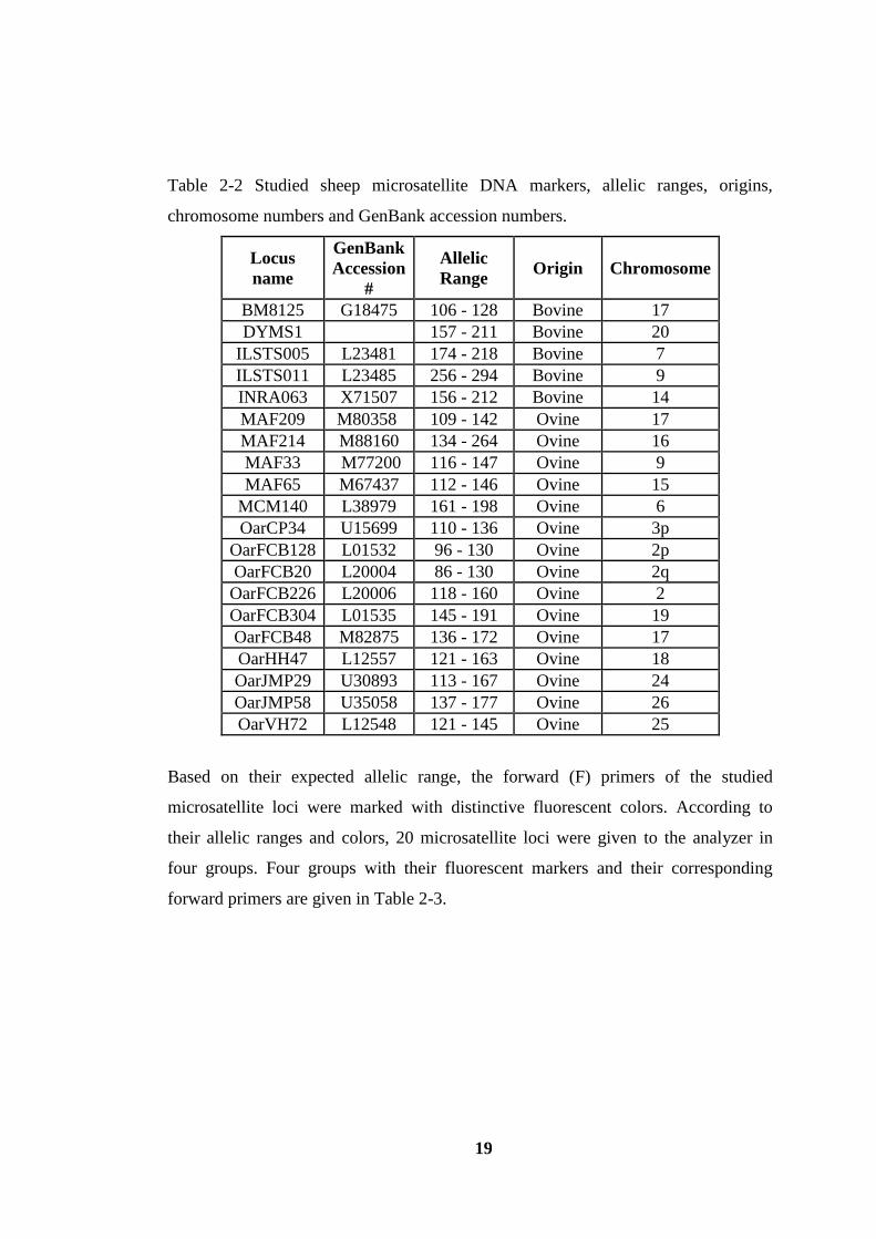
Table 2-2 Studied sheep microsatellite DNA markers, allelic ranges, origins,
chromosome numbers and GenBank accession numbers.
Locus
name
GenBank
Accession
#
Allelic
Range Origin Chromosome
BM8125 G18475 106 - 128 Bovine 17
DYMS1 157 - 211 Bovine 20
ILSTS005 L23481 174 - 218 Bovine 7
ILSTS011 L23485 256 - 294 Bovine 9
INRA063 X71507 156 - 212 Bovine 14
MAF209 M80358 109 - 142 Ovine 17
MAF214 M88160 134 - 264 Ovine 16
MAF33 M77200 116 - 147 Ovine 9
MAF65 M67437 112 - 146 Ovine 15
MCM140 L38979 161 - 198 Ovine 6
OarCP34 U15699 110 - 136 Ovine 3p
OarFCB128 L01532 96 - 130 Ovine 2p
OarFCB20 L20004 86 - 130 Ovine 2q
OarFCB226 L20006 118 - 160 Ovine 2
OarFCB304 L01535 145 - 191 Ovine 19
OarFCB48 M82875 136 - 172 Ovine 17
OarHH47 L12557 121 - 163 Ovine 18
OarJMP29 U30893 113 - 167 Ovine 24
OarJMP58 U35058 137 - 177 Ovine 26
OarVH72 L12548 121 - 145 Ovine 25
Based on their expected allelic range, the forward (F) primers of the studied
microsatellite loci were marked with distinctive fluorescent colors. According to
their allelic ranges and colors, 20 microsatellite loci were given to the analyzer in
four groups. Four groups with their fluorescent markers and their corresponding
forward primers are given in Table 2-3.

20
Table 2-3 Microsatellite groups.
FAM HEX TET
Group 1 OarJMP29 OarFCB20
OarFCB48
OarJMP58
ILSTS005
Group 2 OarFCB128
INRA63
BM8125
OarFCB304
MAF33
MAF214
Group 3
MAF65
MCM140
ILSTS011
MAF209 DYMS1
OarCP34
Group 4 OarFCB226 OarVH72 OarHH47
The sequence of forward and reverse primers of studied 20 microsatellite loci are
presented in Appendix B.
Here detailed PCR conditions are given only for Group I (multiplex - 5 loci) as an
example. Doğan (2009) gave the detailed information of the procedure of PCR
experiments for each group. The general ingredients of the PCR mixture are
presented in the Table 2-4 as follows:
Table 2-4 Constituents of the PCR mixture.
Constituent Stock Solution Final
Concentration Added Volume
dH2O (nuclease-free) - - Up to 15 µL
Buffer 10x 1X 1.5 µL
MgCl2 25 mM 1-4 mM 1.2 µL
dNTP 5 mM 200 µM of each 0.6 µL
Primer (5mM)
200pmol/ µL
(0.2 mM)
10pmol/ µL ~0.6 µL
DNA Varies 10pg-1µg/50 µL 2.5 µL
Taq polymerase 5U/ µL 1u/ µL 0.2 µL
Total volume - - 15 µL

21
Amplification parameters depend greatly on the template, primers and amplification
apparatus used. A sample PCR amplification conditions for group I (5 loci) are
shown in the Table 2-5 as follows:
Table 2-5 PCR amplification protocol for group I loci
PCR step Temperature
(ºC) Time # of Cycle
Initial
Denaturation
94 ºC 2,5 min. 1X
Denaturation 94 ºC 20 sec.
35 X Annealing 57 ºC 35 sec.
Extension 72 ºC 45 sec.
Final Extension 72 ºC 20 min. 1X
Incubation 4 ºC ∞ 1X
2% agarose gels (with 0.5X Tris buffer) were used to check the PCR products for
amplification. Usually 3 µL of DNA samples are mixed with 3 µL of 3X loading dye
(bromophenol blue, sucrose), for each PCR product. 100 volts of electric was applied
to the gels for 1 hour on the horizontal tank that contains 0.5X Tris buffer. To make
the specific PCR product bands visible, for about half an hour, the gels are placed in
a solution that contains EtBr. After that the gels were observed under UV light with
Vilber Lourmat CN-3000.WL displaying device.
In order to size the fragments, the microsatellite PCR products were analyzed on an
automated Applied Biosystems ABI310™ DNA Analyzer by using PE Tamra 350™
internal size standard. For analysis of the fragments from electropherograms and data
collection, Applied Biosystems Peak Scanner™ Software v1.0 was used.

22
2.3 Data Analysis
As explained in the Discussion chapter of this thesis, the microsatellite
markers have high error probability. Therefore, before the analysis, the reliability of
the data was measured and then the consecutive analyses were performed. During the
analysis, several bioinformatics tools were used. However, the main difficulty in this
step was that the output of one tool does not conform to the input of another.
Therefore, to solve this interoperability problem, necessary wrappers/converters were
implemented in Java. Two Java classes were implemented. The first one converts the
output of FreeNA tool to the input of POPTREE2 program and the second Java
wrapper translates a proprietary Excel format to the input format of FSTAT Tool.
These Java classes are given in Appendix E.
2.3.1 Reliability of the Microsatellite Data
Null Alleles
Although microsatellites are highly informative, the incidences of genotyping errors
are also commonly arise during amplification or scoring processes. In certain
populations, when the template DNA is damaged or there are some mutations at the
annealing site of the primer, null alleles occur. The failure of detecting null alleles
may results in an underestimation of within-population genetic diversity (Paetkau
and Strobeck, 1995) and thus an overestimation of FST and genetic distance values
between populations (Paetkau, et al., 1997). Inbreeding, assortative mating or
Wahlund effects usually cause similar deviations. In spite of that, some common
error sources such as short allele dominance; stuttering and null alleles have their
own specific allelic features like deficiencies and excesses of particular genotypes.
Hence, deviations due to the various genotyping errors can be distinguished from
those caused by nonpanmixia (Cock Van, et al., 2004).
For these reasons, in microsatellite studies, the first thing that should be done to
check the incidence of genotyping errors is to screen the data with null allele

23
frequency estimators. Various null allele frequency estimators making use of this
property have been developed (Dempster, et al. 1977; Chakraborty, et al. 1992;
Brookfield, 1996). In 2007, Chapuis and Estoup developed a new tool namely FST
Refined Estimation by Excluding Null Alleles (ENA): FreeNA, which uses the
expectation maximization algorithm of Dempster et al.‟s (1977).
In this study, occurrences of null alleles are tested using FreeNA software (Chapuis,
and Estoup, 2007).
Linkage disequilibrium
D is used a measure of the deviation from random association between alleles at two
loci (Lewontin and Kojima, 1960). D is known as the coefficient of linkage
disequilibrium and is defined in the case of two loci that each have two alleles as:
D = (G1G4) – (G2G3)
where G1, G2, G3 and G4 be the frequency of the four gametes AB, Ab, aB, and ab
respectively.
The population is called as in linkage equilibrium (D=0), if the alleles are associated
at random in population. On the other hand, the alleles in two loci are not associated
randomly if D is not zero. In this case the population is called as in linkage
disequilibrium. Since the employed loci are not close on the sheep genome, in the
present study none of the loci pairs are expected to be in linkage disequilibrium.
However, if sample of the breeds were composed of closely related individuals then
presence of linkage disequilibrium would be observed.
Linkage disequilibrium estimations were (for total sample size and for each breed
separately) done based on 19 loci with FSTAT V.2.9.3 package program (Goudet,
2001).

24
2.3.2 Methods used for the Statistical Analyses
In this section, statistical analyses methods were listed. The software used for these
analyses were given in each part after general explanations of the methods.
2.3.2.1 Estimation of Genetic Variation
In this study the main objective is to compare the amount of genetic variation in
different breeds. Allelic and heterozygosity analyses are the two approaches to
examine within population (breed) variation (Allendorf and Luikart, 2007).
2.3.2.1.1 Allelic variation
Allelic richness, polymorphism information content and private alleles of the data
were investigated for the estimation of allelic variation, and hence genetic variation
within the breeds.
2.3.2.1.1.1 Allelic Richness
To measure the genetic variation, a commonly used method is to examine the total
number of alleles. This measure is more sensitive than heterozygosity to the loss of
genetic variation caused by small population size and this feature makes it an
important measure of the long-term evolutionary potential of populations (Allendorf,
1986). The number of distinct alleles depends heavily on sample size, and it can be
difficult to interpret when sample sizes differ across populations, since there are
several low frequency alleles in natural populations. To eliminate this drawback,
„allelic richness‟ can be used. It is defined as a measure of allelic diversity that
considers the sample size (Mousadik and Petit, 1996) or the number of distinct
alleles expected in a random sub-sample of size g drawn from the population (Petit,
et al. 1998). In allelic richness calculation unequal samples are trimmed to the same
standardized sample size, g, and populations are compared by considering the
estimates of allelic richness. Allelic richness can be denoted by R(g).
25
Allelic richness estimations in terms of 19 loci were calculated with FSTAT V.2.9.3
package program (Goudet, 2001).
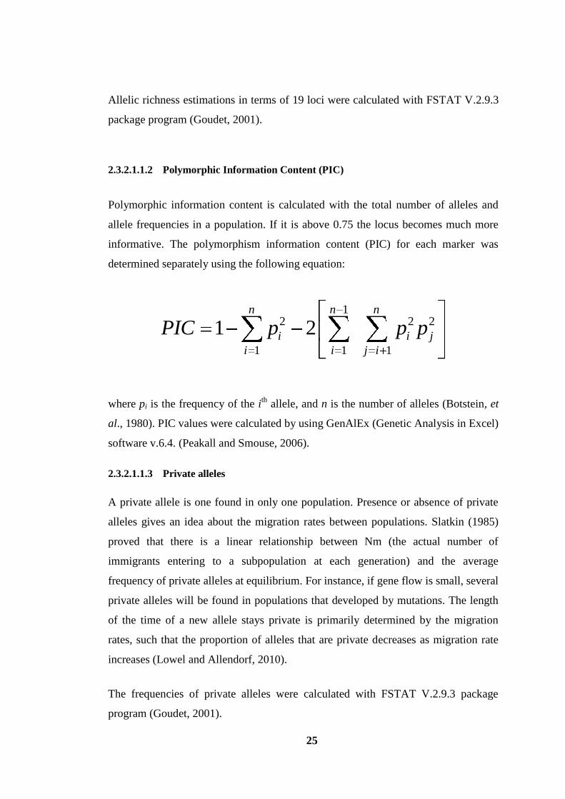
2.3.2.1.1.2 Polymorphic Information Content (PIC)
Polymorphic information content is calculated with the total number of alleles and
allele frequencies in a population. If it is above 0.75 the locus becomes much more
informative. The polymorphism information content (PIC) for each marker was
determined separately using the following equation:
12 2 2
1 1 1
1 2n n n
i i j
i i j i
PIC p p p
where pi is the frequency of the ith
allele, and n is the number of alleles (Botstein, et
al., 1980). PIC values were calculated by using GenAlEx (Genetic Analysis in Excel)
software v.6.4. (Peakall and Smouse, 2006).
2.3.2.1.1.3 Private alleles
A private allele is one found in only one population. Presence or absence of private
alleles gives an idea about the migration rates between populations. Slatkin (1985)
proved that there is a linear relationship between Nm (the actual number of
immigrants entering to a subpopulation at each generation) and the average
frequency of private alleles at equilibrium. For instance, if gene flow is small, several
private alleles will be found in populations that developed by mutations. The length
of the time of a new allele stays private is primarily determined by the migration
rates, such that the proportion of alleles that are private decreases as migration rate
increases (Lowel and Allendorf, 2010).
The frequencies of private alleles were calculated with FSTAT V.2.9.3 package
program (Goudet, 2001).

26
2.3.2.1.2 Heterozygosity
The average expected (Hardy-Weinberg) heterozygosity at n loci within a population
is the best general measure of genetic variation within-populations (Allendorf and
Luikart, 2007).
2
1
1n
e i
i
H p
Square of p gives the expected frequency of homozygotes for pth
allele of ith
locus
and by introducing all of the loci (1 to n), total amount of expected homozygosity is
subtracted from 1, which gives expected heterozygosity.
Estimation of HE generally is not affected by sample size and even a few individuals
are sufficient for estimating HE if a large number of loci are examined (Gorman and
Renzi, 1979). Furthermore, it is robust to the presence of null alleles (Drury, et al.,
2009).
Expected (Hexp) heterozygosity were estimated using GENETIX Software v. 4.05
(Belkhir, et al., 1996–2004; http://univ-montp2.fr/~genetix) for each population-by-
locus combination and for each population estimates. Deviations from Hardy–
Weinberg equilibrium (HW) were assessed for each locus-population combination
using a Markov chain of 10 000 steps and 1000 dememorization steps and to correct
for the multiplicity of comparisons Bonferroni correction of 0.05 divided by the
number of tests was used.
2.3.2.2 F-statistics: FIS and Pairwise FST Values
F-statistics (inbreeding coefficients) developed by Wright (1965) and extended by
Nei (1977) is the oldest and most widely used method to measure the genetic
differentiation within and between populations (Allendorf and Luikart, 2007).

27
Usually, the genotype frequencies in populations do not follow Hardy-Weinberg
equilibrium frequencies in nature and F statistics uses these deviations to measure the
inbreeding (which is the tendency for mates to be closely related) within populations.
One of these inbreeding coefficients, FIS is a measure of departure from Hardy-
Weinberg proportions within local subpopulations and estimated by the formula:
1 OIS
S
HF
H
where Ho is the mean observed heterozygosity over all sub-populations, and HS is the
mean expected heterozygosity over all sub-populations.
FIS will be positive meaning there is inbreeding in the examined population which
cause heterozygotes deficiency. On the other hand, FIS will be negative when there is
migration from outside of the population cause an excess of heterozygotes.
FST is a measure of genetic divergence among sub-populations and can be used as a
distance measure. It can be calculated by the formula:
1ST
T
HsF
H
where HT is the expected heterozygosity if the entire base population were panmictic
(random mating is observed) and HS is the mean expected heterozygosity over all
sub-populations. With using two populations each time, it can be used as a distance
matrix to compare pairwise differences among sub-populations.

28
FST will be between 0, when populations have equal allele frequencies, and 1, when
populations are fixed for different alleles. That‟s why, FST called as fixation index,
sometimes.
F indices proposed by Wright (1965) does not consider the unequal finite sample
sizes and there is some disagreement on the interpretation of the quantities and on the
method of evaluating them. Weir and Cockerham (1984) revised the F coefficients
in order to unify various estimation formulas so that they are suited to small data
sets.
In this study, Weir and Cockerham's (1984) unbiased estimator approach is used to
examine the sample structure, permuted 1000 times over loci to test deviations from
Hardy-Weinberg proportions.
FST values by pairwise comparisons of thirteen breeds and FIS values within each
breeds were calculated by FSTAT V.2.9.3 package program (Goudet, 2001),
Significance of those were tested by applying 1000 random permutations and to
correct for the multiplicity of comparisons Bonferroni correction of 0.05 divided by
the number of tests was used.
2.3.2.3 Genetic Distance Estimations and Phylogenetic Tree Construction
F statistics make a pairwise comparison to provide the structure of the populations.
However, while doing those pairwise comparisons, they do not take account all the
data, instead they take only the data of the two populations compared. Therefore, to
define the genetic differences between the populations in entire pool of the data
“genetic distances” defined by various scientists can be used, which yield a genetic
distance matrix. In the present study two different genetic distance measures are
employed.
29
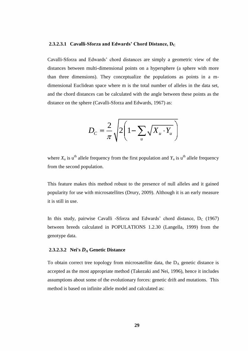
2.3.2.3.1 Cavalli-Sforza and Edwards‟ Chord Distance, DC
Cavalli-Sforza and Edwards‟ chord distances are simply a geometric view of the
distances between multi-dimensional points on a hypersphere (a sphere with more
than three dimensions). They conceptualize the populations as points in a m-
dimensional Euclidean space where m is the total number of alleles in the data set,
and the chord distances can be calculated with the angle between these points as the
distance on the sphere (Cavalli-Sforza and Edwards, 1967) as:
22 1C u u
u
D X Y
where Xu is uth
allele frequency from the first population and Yu is uth
allele frequency
from the second population.
This feature makes this method robust to the presence of null alleles and it gained
popularity for use with microsatellites (Drury, 2009). Although it is an early measure
it is still in use.
In this study, pairwise Cavalli -Sforza and Edwards‟ chord distance, DC (1967)
between breeds calculated in POPULATIONS 1.2.30 (Langella, 1999) from the
genotype data.
2.3.2.3.2 Nei's DA Genetic Distance
To obtain correct tree topology from microsatellite data, the DA genetic distance is
accepted as the most appropriate method (Takezaki and Nei, 1996), hence it includes
assumptions about some of the evolutionary forces: genetic drift and mutations. This
method is based on infinite allele model and calculated as:
30
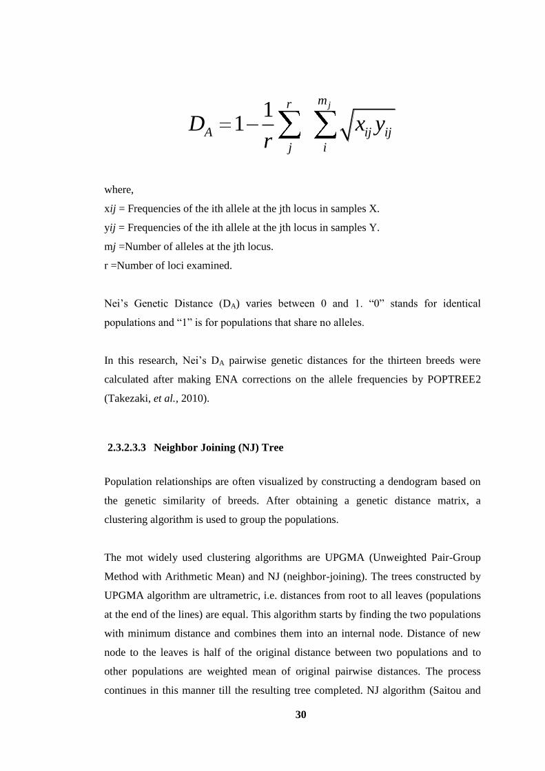
11
jmr
A ij ij
j i
D x yr
where,
xij = Frequencies of the ith allele at the jth locus in samples X.
yij = Frequencies of the ith allele at the jth locus in samples Y.
mj =Number of alleles at the jth locus.
r =Number of loci examined.
Nei‟s Genetic Distance (DA) varies between 0 and 1. “0” stands for identical
populations and “1” is for populations that share no alleles.
In this research, Nei‟s DA pairwise genetic distances for the thirteen breeds were
calculated after making ENA corrections on the allele frequencies by POPTREE2
(Takezaki, et al., 2010).
2.3.2.3.3 Neighbor Joining (NJ) Tree
Population relationships are often visualized by constructing a dendogram based on
the genetic similarity of breeds. After obtaining a genetic distance matrix, a
clustering algorithm is used to group the populations.
The mot widely used clustering algorithms are UPGMA (Unweighted Pair-Group
Method with Arithmetic Mean) and NJ (neighbor-joining). The trees constructed by
UPGMA algorithm are ultrametric, i.e. distances from root to all leaves (populations
at the end of the lines) are equal. This algorithm starts by finding the two populations
with minimum distance and combines them into an internal node. Distance of new
node to the leaves is half of the original distance between two populations and to
other populations are weighted mean of original pairwise distances. The process
continues in this manner till the resulting tree completed. NJ algorithm (Saitou and

31
Nei, 1987) is different than UPGMA in that branch lengths of the tree can be
different (non-ultrametric), therefore can give additional information about the
relationship between populations. It combines populations that are closest to each
other and also furthest from the rest. It is a fast method even for very large data sets.
Furthermore it is useful for bootstrap analysis. Bootstrap analysis is a sampling
method which is widely used when sampling distribution is unknown to determine
the statistical error. To reach this aim, it constructs hundreds of replicate trees. . In
NJ tree construction, by sequentially finding the neighbors it helps to minimize the
total length of the tree. Since NJ tree does not assume equal rate of evolution of the
breeds after the divergence, NJ method performs better under non-uniform rates
either among lineages or among sites.
The pairwise DC chord distances were used to build NJ tree, to visualize the genetic
relationships among the breeds. In this analysis, Treeview was used for visualization
of the tree (Page, 1996) and POPULATIONS 1.2.30 (Langella, 1999) was used for
its construction.
Also Nei's DA genetic distance was used to build NJ trees with ENA correction and
without ENA correction with the software program POPTREE2 (Takezaki, et al.,
2010).
2.3.2.4 Analysis of Molecular Variance (AMOVA)
In F statistics gene frequencies are compared among breeds, however, from
molecular data, not only the frequency of molecular markers but also the amount of
mutational differences between different genes can be obtained. Instead of
Mendelian gene frequencies, a method that analyses differences between molecular
sequences is very useful to estimate the population differentiation. One can achieve
this by using Analysis of Molecular Variance (AMOVA) which estimate population
differentiation directly from molecular data and testing hypotheses about such
differentiation. Several kinds of molecular data, such as microsatellite based data or
direct sequence data can be analyzed with this method (Excoffier, et al., 1992).

32
With AMOVA, any kind of raw molecular data is analyzed as a Boolean vector pi,
that is, a “1 x n” matrix of 1s and 0s, where 1 indicates the presence of a marker and
0 its absence. By subtracting the Boolean vector of one haplotype from another,
Euclidean distances between pairs of vectors are then calculated. For all pairwise
arrangements of Boolean vectors, squared Euclidean distances are calculated and
then set into a matrix, and divided into sub-matrices corresponding to subdivisions
within the population. The data can then be analyzed in a nested analysis of variance
framework. A nested ANOVA differs from a simple ANOVA in that data is arranged
hierarchically and mean squares are computed for groupings at all levels of the
hierarchy. This allows for hypothesis tests of between-group and within-group
differences at several hierarchical levels (Excoffier, et al., 1992)
The design and formulas of the calculation for AMOVA for genotypic data, several
groups of populations, within-individual level as can be seen in the Excoffier et al.‟s
(2006) Arlequin package program is in the table below:
Table 2-6 General AMOVA table for genotypic data, several groups of populations,
within-individual level taken from Arlequin package program (Excoffier et al.,
2006).
Source of Variation Degrees of freedom
Sum of squares (SSD)c Expected mean squares
Among Groups G-1 SSD(AG) '' 2 ' 2 2 22n na b c d
Among Populations / Within Groups
P-G SSD(AP/WG) 2 2 22nb c d
Among Individuals / Within Populations
N-P SSD(AI/WP) 2 22c d
Within Individuals N SSD(WI) 2d
Total 2N-1 SSD(T) 2T

33
where;
SSD (AG): Sum of squared deviations among groups of populations
SSD (AP/WG): Sum of squared deviations among populations, within groups
SSD (AI/WP): Sum of squared deviations among individuals, within populations
SSD (WI): Sum of squared deviations within individuals
SSD (T): Total sum of squared deviations
G: Number of groups in the structure
P: Total number of breeds
N: Total number of gene copies
The variance components can be used to calculate a series of statistics called phi-
statistics ( ), which summarize the degree of differentiation between population
divisions and are analogous to F-statistics, such as CT, SC, IS and
IT corresponds to the differentiation among groups, among populations-within
groups, among individuals-within populations and within individuals, respectively.
Hypothesis about differentiation at corresponding level of a population can be
constructed by F -statistic. Furthermore, these hypotheses can be tested using the null
distribution of the corresponding variance components; if the variance of the
subpopulations does not significantly differ from the null distribution of the variance
of the population, the hypothesis that those subpopulations are differentiated from
the larger population would be rejected.
The data do not perfectly follow a normal distribution; hence the molecular data
consist of Euclidean distances obtained from vectors of 1s and 0s. Therefore
resampling of the data is used to compute the null distribution (Excoffier, et al.
1992). In each iteration, individuals are assigned to a randomly chosen population
while holding the sample sizes constant. Many permutations are made to build the
null distribution to which hypothesis will be tested.
Since the null distributions are obtained by resampling, the individuals from which
haplotypes are sampled should be chosen independently and at random. Because of

34
genetic drift, any one haplotype should not be assumed to be completely
representative of variation among the whole genome. It is therefore important that
the data are derived from an adequate number of markers. Using neutral, non-
selected genetic markers can be a useful means of avoiding the confounding effects
of selection, if neutral markers can be identified.
Populations are assumed to be panmictic and there is no inbreeding. Violation of
these assumptions will result in heterozygote deficiency and if the rates of non-
random mating or inbreeding differ between populations, fixation estimates will be
confounded.
In this study, Arlequin (Excoffier, et al. 2006) package program was used for
AMOVA analysis.
2.3.2.5 Factorial Correspondence Analysis (FCA)
In multidimensional space to see the individuals and to investigate the relationships
between the individuals, the Factorial Correspondence Analysis (FCA) (Lebart, et
al,. 1984) is used. Each individual is represented with respect to the alleles. For each
of the allele the diploid individual can assume 0, 1 or 2. Hence string of “0, 1, 2” will
represent the individuals. The program finds independent axes which are the linear
combinations of the alleles such that the maximum genetic diversity observed within
the total data could be explained by the first axis. The most informative axes are first
three ones (Machugh, et al., 1994). Visualizing on the independent axes for how
individuals are related to each other is an informative way to see the amount of
inertia, distinctness of the breeds and yet relative similarity between the breeds.
GENETIX Software v. 4.05 (Belkhir et al. 1996–2004; http://univ-
montp2.fr/~genetix) was used to obtain three dimensional FCA.
2.3.2.6 Structure Analysis
The STRUCTURE software provides an effective way to illustrate the presence of
population structure and to distinguish distinct genetic populations (Pritchard, et al.,
2000). The underlying assumptions of the model in which there are K populations

35
(where K may be unknown), each of which is characterized by a set of allele
frequencies at each locus. If their genotypes indicate that they are admixed, the
individuals in the sample are assigned jointly to two or more populations. With the
version 2.2 of Structure software, microsatellites, Amplified Fragment Length
Polymorphisms (AFLP), Restriction Fragment Length Polymorphisms (RFLP) and
Single Nucleotide Polymorphisms (SNPs) data sets could be used and analyzed
(Falush, et al., 2007).
The most significant factors to determine for STRUCTURE analysis are the burn in
length, the ancestry model and estimation of K (number of populations).
Burn in length explains how long to run the simulation before collecting data to
make sure that the simulated population reached to drift-mutation equilibrium which
minimizes the starting configuration. Typically a burn in length of > 5N0 is used,
where N0 indicate the initial population size and 10,000 - 100,000 burn-in length is
more than adequate (Falush, et al., 2003).
For the ancestry of individuals, admixture model was performed in this work. This
model is reasonably flexible for many of the complexities of real populations
(Falush, et al., 2003). It assumes that individuals may have mixed ancestry.
There are several methods suggested to estimate K (number of populations). One of
them is the method suggested by Evanno et al. (2005). For the true K, the
distribution of Ln P(D) (or L(K), according to Evanno et al. (2005), do not indicate a
clear mode, but at the true value of K the second order rate of change of the
likelihood function (ΔK = m|L‟‟(K)|/ s[L(K)]) with respect to K ('K) does show a
clear peak.
Another method recently developed and widely used (Tapio, et al., 2010) is based on
testing the similarity between the results of individual runs for each different value of
K. At the maximum similarity, it is argued that the correct K is obtained.

36
Both models were used in this research. The population structure and the level of
admixture in the sheep breeds were analyzed by using STRUCTURE v2.2.3
(Pritchard, et al., 2000). The program is available at
http://pritch.bsd.uchicago.edu/software.
2.3.2.7 Delaunay Network Analysis
By the application of Thiessian polygons, the Delaunay network can be constructed
(Monmonier, 1973; Brassel and Reif, 1979). For this purpose, first, the map of the
study is generated and it is divided into regions, which are distribution areas of the
breeds studied. After that, points are put in the middle of these regions for the
representation of the regions or breeds. Then, by connecting the points in the outer
regions, the outer boundary of the study is drawn. Finally, the internal points are
connected through "shortest distance" criterion and the “Delaunay Network" is
generated.
To identify possible genetic barriers, pair-wise genetic differences among the breeds
are marked on the related edges of the triangles linking the points (Brassel and Reif,
1979). A perpendicular is drawn to the triangle edges in the outer boundary having
the longest pair-wise genetic distance, and the cursors is either in the neighboring
triangle or outside of the outer polygon. The perpendicular line drawing goes on till
outside of the polygon, which is the barrier, is reached. The drawing of the second
barrier begins from one of the edges of the outer polygon uncrossed by the first
barrier and has the longest pair-wise genetic distance. Drawing of the second barrier
goes on until it crosses the first barrier or it is out of the polygon. The drawing of the
barriers goes on until all the edges of the outer polygon are tested. If the barrier is
inside of the polygon, but has circles inside the polygon, then it means there is no
barrier. The order of the barriers ranks the height of the barriers or the importance of
the barriers.

37
CHAPTER 3
RESULTS
3.1 Experimental Results
3.1.1 DNA Extraction and Polymerase Chain Reaction (PCR) Results
The DNA was extracted by standard phenol:chloroform DNA extraction protocol
(Sambrook, et al., 1989). The extracted DNA was run on 0.8 % agarose gel;
obtained bands were visualized by Vilber Lourmat CN-3000.WL displaying device.
Brightness and the thickness of the bands were controlled to determine the suitability
of the samples in terms of quality and quantity for further use. DNA should be
diluted as total amount of template DNA in Polymerase Chain Reaction (PCR) tubes
should be between 100-50 ng. Necessary dilutions were performed according to the
concentration of the samples through comparing them with eye against the standard λ
DNA size marker as explained in Chapter 2 of the presented thesis.
In Figure 3-1 and Figure 3-2, examples of gels before and after the required DNA
concentrations were reached.
Figure 3-1 DNA bands before adjustment of concentrations of the DNAs in 0.8%
agarose gel. Here λ DNA size markers were used and the first 22 individuals of
Akkaraman breed were checked.

38
Figure 3-2 DNA bands after adjustment of concentrations of the DNAs in 0.8%
agarose gel. Here λ DNA size markers were used and the first 22 individuals of
Akkaraman breed were checked.
Through PCR, the amplification of the 20 microsatellite loci was achieved and the
obtained DNA fragments were run in 2% agarose gel to control the success of the
amplification process. In each case, to check the existence of contamination, one well
was allocated to negative control where the concentrations of the solutions were
similar to those of the other wells yet instead of DNA only water added.
A sample result from three microsatellite loci (OarFCB20, OarJMP58 and
ILSTS005) studies as multiplex PCR was given in Figure 3-3. In this gel, to assign
each microsatellite markers, known ranges of molecular weight of the PCR products
were used.

39
Figure 3-3 Control of the multiplex PCR products of three loci (OarFCB20,
OarJMP58 and ILSTS005). C represents the negative control and first 8 individuals
of Morkaraman breed was studied here.
3.1.2 Microsatellite Analyses
In order to size the fragments, the microsatellite PCR products were analyzed on an
automated Applied Biosystems ABI310™ DNA Analyzer by using PE Tamra 350™
internal size standard. For analysis of the fragments from electropherograms and data
collection, Applied Biosystems Peak Scanner™ Software v1.0 was used. The
molecular weight of the PCR products and fluorescence tag of each marker was
known and this information was used to distinguish and detect the microsatellite
markers on these electropherograms. The examples of electropherogram resulted
from a raw data with “.fsa” extension by using three microsatellite loci analyzed in
one group was presented in Figure 3-4, as an example.
Figure 3-4 Microsatellite electropherogram representing three loci: FCB20,
OarCP34, VH72, obtained by Applied Biosystems Peak Scanner™ Software v1.0.
The peaks corresponding to each loci were indicated by arrows and the names of the
loci.

40
3.2 Statistical Analyses
Results of the allelic readings from 20 microsatellite loci in 13 Turkish sheep breeds
(n=628) were obtained. Genotypes of 628 individuals based on their 20 loci have
been provided in CD attached to this study. Only for the breed Norduz genotypes
were given as an example in Appendix C.
3.2.1 Reliability of the Microsatellite Data
Before carrying out the statistical analyses, reliability of microsatellite data was
assessed. For this purpose, first, the number of alleles obtained in the present study
was compared with those obtained in a 5th frame European Union (EU) project: with
the acronym ECONOGENE (http://www.econogene.eu). ECONOGENE was
covering 57 sheep breeds from Europe, and Middle East. In their data there were 4
breed samples from Turkey. Therefore allele numbers were obtained for the whole
data of ECONOGENE and ECONOGENE data only for four Turkish breeds
(Akkaraman, Karayaka, Dağlıç and Morkaraman). Allele numbers usually increase
with the number of studied breeds. Therefore, allele numbers of the present study
was expected to be between those of full ECONOGENE study and ECONOGENE
Turk study. Table 3-1, for the same microsatellite loci, presented the number of
alleles observed by different studies or combinations of breeds. It can be seen that
except MAF 214 locus, the number of observed alleles are in good fit with those of
the previously observed ones based on the aforementioned expectation.
Then a recently (Chapuis and Estaup, 2007) published software FreeNA which
detects the null alleles (they are alleles but could not be observed) was employed to
observe the possible effects of presence of null alleles. In Table 3-2 estimated null
allele frequencies were given for each locus and breed. Excluding Null Allele (ENA)
corrections were made on the remaining allele frequencies according to the
frequencies of the null alleles; and now data can be used for some further analyses to
judge the effect of null allele presence. Frequencies bigger than 0.05 threshold level
are considered to be low reliability for the further analysis. They are highlighted with
grey in Table 3-2. MAF 214 again seemed to be a locus with a non-reliable data for

41
which extremely high null allele frequencies were observed in 11 of 13 examined
breeds.
Table 3-1 Comparative representation of allele numbers obtained from the same 20
microsatellite loci studied in ECONOGENE with 57, in ECONOGENE Europe with
48 European, in ECONOGENE Turk with 4 Turkish and in TURKHAYGEN-I (this
study) with 13 Turkish sheep breeds.
Loci ECONOGENE
ECONOGENE
Europe
ECONOGENE
Turk TURKHAYGEN-I
BM8125 12 12 8 10
DYMS1 24 24 16 18
ILSTS 011 14 14 6 10
ILSTS005 17 16 9 13
INRA063 27 26 19 19
MAF209 16 16 11 14
MAF214 41 35 16 6
MAF33 15 15 11 14
MAF65 17 16 12 13
MCM 140 17 17 13 13
OarCP34 14 14 8 8
OarFCB128 14 13 11 16
OarFCB20 20 19 14 16
OarFCB226 18 17 14 15
OarFCB304 24 24 16 23
OarFCB48 - - - 13
OarHH47 20 20 14 14
OarJMP29 27 27 20 18
OarJMP58 22 22 15 19
OarVH72 10 10 8 9
Another test for the reliability of data was carried out by screening the presence of
linkage disequilibrium of the loci calculated in FSTAT V.2.9.3 (Goudet, 2001)
package program. Results of the pairwise comparison of loci for the total data are
given in the Table 3-3 below and those of the breed based pairwise comparison of
loci were given in Appendix D.
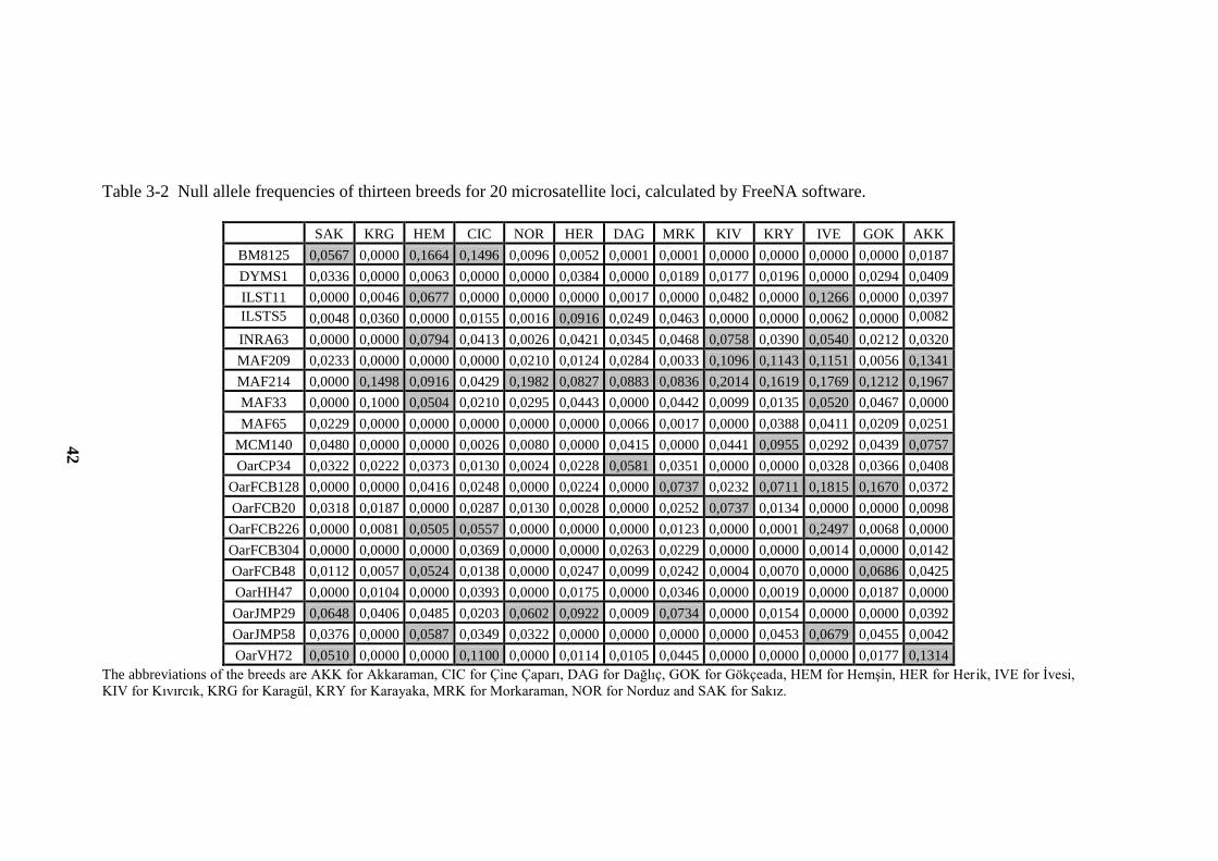
42
Table 3-2 Null allele frequencies of thirteen breeds for 20 microsatellite loci, calculated by FreeNA software.
SAK KRG HEM CIC NOR HER DAG MRK KIV KRY IVE GOK AKK
BM8125 0,0567 0,0000 0,1664 0,1496 0,0096 0,0052 0,0001 0,0001 0,0000 0,0000 0,0000 0,0000 0,0187
DYMS1 0,0336 0,0000 0,0063 0,0000 0,0000 0,0384 0,0000 0,0189 0,0177 0,0196 0,0000 0,0294 0,0409
ILST11 0,0000 0,0046 0,0677 0,0000 0,0000 0,0000 0,0017 0,0000 0,0482 0,0000 0,1266 0,0000 0,0397
ILSTS5 0,0048 0,0360 0,0000 0,0155 0,0016 0,0916 0,0249 0,0463 0,0000 0,0000 0,0062 0,0000 0,0082
INRA63 0,0000 0,0000 0,0794 0,0413 0,0026 0,0421 0,0345 0,0468 0,0758 0,0390 0,0540 0,0212 0,0320
MAF209 0,0233 0,0000 0,0000 0,0000 0,0210 0,0124 0,0284 0,0033 0,1096 0,1143 0,1151 0,0056 0,1341
MAF214 0,0000 0,1498 0,0916 0,0429 0,1982 0,0827 0,0883 0,0836 0,2014 0,1619 0,1769 0,1212 0,1967
MAF33 0,0000 0,1000 0,0504 0,0210 0,0295 0,0443 0,0000 0,0442 0,0099 0,0135 0,0520 0,0467 0,0000
MAF65 0,0229 0,0000 0,0000 0,0000 0,0000 0,0000 0,0066 0,0017 0,0000 0,0388 0,0411 0,0209 0,0251
MCM140 0,0480 0,0000 0,0000 0,0026 0,0080 0,0000 0,0415 0,0000 0,0441 0,0955 0,0292 0,0439 0,0757
OarCP34 0,0322 0,0222 0,0373 0,0130 0,0024 0,0228 0,0581 0,0351 0,0000 0,0000 0,0328 0,0366 0,0408
OarFCB128 0,0000 0,0000 0,0416 0,0248 0,0000 0,0224 0,0000 0,0737 0,0232 0,0711 0,1815 0,1670 0,0372
OarFCB20 0,0318 0,0187 0,0000 0,0287 0,0130 0,0028 0,0000 0,0252 0,0737 0,0134 0,0000 0,0000 0,0098
OarFCB226 0,0000 0,0081 0,0505 0,0557 0,0000 0,0000 0,0000 0,0123 0,0000 0,0001 0,2497 0,0068 0,0000
OarFCB304 0,0000 0,0000 0,0000 0,0369 0,0000 0,0000 0,0263 0,0229 0,0000 0,0000 0,0014 0,0000 0,0142
OarFCB48 0,0112 0,0057 0,0524 0,0138 0,0000 0,0247 0,0099 0,0242 0,0004 0,0070 0,0000 0,0686 0,0425
OarHH47 0,0000 0,0104 0,0000 0,0393 0,0000 0,0175 0,0000 0,0346 0,0000 0,0019 0,0000 0,0187 0,0000
OarJMP29 0,0648 0,0406 0,0485 0,0203 0,0602 0,0922 0,0009 0,0734 0,0000 0,0154 0,0000 0,0000 0,0392
OarJMP58 0,0376 0,0000 0,0587 0,0349 0,0322 0,0000 0,0000 0,0000 0,0000 0,0453 0,0679 0,0455 0,0042
OarVH72 0,0510 0,0000 0,0000 0,1100 0,0000 0,0114 0,0105 0,0445 0,0000 0,0000 0,0000 0,0177 0,1314
The abbreviations of the breeds are AKK for Akkaraman, CIC for Çine Çaparı, DAG for Dağlıç, GOK for Gökçeada, HEM for HemĢin, HER for Herik, IVE for Ġvesi,
KIV for Kıvırcık, KRG for Karagül, KRY for Karayaka, MRK for Morkaraman, NOR for Norduz and SAK for Sakız.
42

43
Table 3-3 P-value for genotypic disequilibrium of 19 microsatellite loci based on 3420 permutations.
After Bonferroni corrections adjusted P-value for 5% nominal level is: [0.05/171] = 0.00029.
43 4
3

44
Only the loci MAF33 and OarFCB128 have a significant disequilibrium. If examined
for each breed in detail in Appendix D, this disequilibrium was seen only in Kıvırcık.
Since chosen loci were either on different chromosomes or located distantly on the
same chromosome, linkage disequilibrium was not expected. Linkage disequilibrium
would indicate error in genotyping or presence of closely related individuals in the
samples. Indeed Kıvırcık had a significant deviation from Hardy- Weinberg (H-W)
equilibrium. Result of the present study: absence of linkage disequilibrium also
increases the confidence of the reliability on genotyping and data.
Finally, the results of 4 loci (INRA63, MAF65, OarFCB20 and OarFCB304; which
are used by ISAG test committee) were tested by ISAG results. If only the wrong
genotyping were counted it was observed that 80% of the genotypes were correctly
genotyped. Therefore, whole readings were repeated and each locus was studied by
only one student. In the Discussion part of the thesis possible sources of errors in
microsatellite readings are discussed.
3.2.2 Breed Based Analyses
Here, breeds were considered as the study unit. Out of 20 studied loci, MAF214 was
excluded from the analyses.
3.2.2.1 Genetic Variation Analyses
Genetic variation of the breeds was mainly represented by allelic variation and
heterozygosity.
3.2.2.1.1 Allelic Variation
Allelic variation can be assessed by the analyses of allelic richness, polymorphism
information content and private alleles.

45
3.2.2.1.1.1 Allelic Richness
In total, 281 alleles were detected at the 20 microsatellite loci analyzed. Table 3-1
provided the total number of alleles observed for the 20 loci. The maximum number
of alleles for single locus is 23 for OarFCB304. On the other hand, the minimum was
8 for OarCP34. Since MAF214 was excluded, its allele number was not taken into
account.
The allelic richness calculated for each locus in each breed and the averages are
presented in Table 3-4. The maximum and minimum allelic richness of loci were
14.79 (INRA063) and 6.58 (BM8125). On the other hand, the maximum and
minimum allelic richness of breeds were 9.81 (Herik) and 7.87 (Sakız).

46
Table 3-4 Allelic richness calculated for each locus in each breed, the mean number of alleles observed for each breed and for each locus.
Locus SAK KRG HEM CIC NOR HER DAG MRK KIV KRY IVE GOK AKK Overall
BM8125 6,78 6,54 7,67 5,94 5,53 7,51 5,80 4,84 5,85 5,94 7,53 6,15 5,62 6,58
DYMS1 9,67 11,68 10,14 8,43 12,37 11,26 10,36 11,76 10,89 12,15 11,45 10,21 10,92 12,52
ILST11 5,99 5,54 7,48 8,39 5,75 6,63 8,60 6,73 7,86 7,14 6,88 4,98 4,89 7,66
ILSTS5 5,86 6,18 6,50 3,99 7,21 5,49 6,84 7,86 4,71 6,03 5,69 5,83 5,47 6,74
INRA63 6,20 7,14 14,59 12,59 9,79 15,62 14,47 12,49 14,08 12,88 11,95 13,83 16,31 14,79
MAF209 7,69 5,85 11,28 10,00 8,14 8,28 8,70 8,42 8,78 10,61 8,48 9,36 11,24 10,01
MAF33 7,05 11,32 11,43 9,17 8,45 9,11 11,00 7,02 7,96 10,27 9,02 8,49 6,97 10,97
MAF65 5,80 4,89 6,61 5,94 8,83 8,29 7,41 9,57 9,48 8,38 10,46 9,81 6,98 8,97
MCM140 7,17 8,90 9,17 8,43 9,50 11,99 12,00 11,26 10,79 10,76 9,73 9,38 10,59 10,80
OarCP34 6,49 6,84 6,95 7,00 6,88 6,75 7,58 6,00 7,88 6,62 5,99 7,20 7,57 7,16
OarFCB128 6,76 6,38 10,85 8,55 6,72 12,31 7,00 8,60 8,41 10,09 7,80 10,78 7,60 12,52
OarFCB20 8,32 9,41 11,22 7,50 10,86 10,78 11,27 10,85 11,45 7,99 12,55 8,97 12,56 10,95
OarFCB226 11,78 10,06 13,83 13,30 12,35 11,65 12,89 10,33 11,14 10,74 11,29 9,14 9,60 12,85
OarFCB304 12,36 11,62 9,84 7,92 13,12 11,64 11,67 13,97 10,38 12,41 13,85 8,19 10,21 12,96
OarFCB48 6,73 8,99 7,46 6,70 10,95 7,44 8,90 8,77 9,54 8,30 8,96 8,48 7,91 9,28
OarHH47 10,60 9,76 11,09 9,58 11,67 12,17 11,36 11,38 12,09 11,10 11,56 12,85 12,14 12,12
OarJMP29 8,60 8,63 8,36 8,43 10,32 8,78 7,53 8,38 11,03 10,70 11,15 9,70 10,89 11,56
OarJMP58 7,89 9,95 7,91 8,31 8,77 13,10 10,19 10,61 10,73 11,06 11,58 13,04 11,86 11,89
OarVH72 7,86 7,63 7,88 6,99 8,53 7,61 8,77 8,58 7,88 5,94 7,58 5,00 6,89 8,17
Overall 7,87 8,28 9,49 8,27 9,25 9,81 9,60 9,34 9,52 9,43 9,66 9,02 9,27 9,79
Based on min. sample size of: 30 diploid individuals.
The abbreviations of the breeds are AKK for Akkaraman, CIC for Çine Çaparı, DAG for Dağlıç, GOK for Gökçeada, HEM for HemĢin, HER for Herik, IVE for Ġvesi,
KIV for Kıvırcık, KRG for Karagül, KRY for Karayaka, MRK for Morkaraman, NOR for Norduz and SAK for Sakız.
64
46

47
3.2.2.1.1.2 Polymorphism Information Content (PIC)
According to the Table 3-5, least informative loci are BM8125 and ILSTS005 with
PIC values of 0.5754 and 0.5815, respectively. This result is in accordance with the
allelic richness table, where the loci BM8125 and ILSTS005 had the lowest two
allelic richness values. The maximum informative locus is OarFCB20 with a PIC
value of 0.8315. It can be seen from this table that on the average all of these loci
have high information content in Turkish sheep breeds. Hence, they were suitable for
studying genetic diversity of Turkish sheep breeds and they were strongly
recommended for future similar studies.
Table 3-5 PIC of each locus and breed.
Locus SAK KRG HEM CIC NOR HER DAG MRK KIV KRY IVE GOK AKK Overall
BM8125 0,60 0,55 0,71 0,74 0,58 0,61 0,49 0,47 0,46 0,68 0,57 0,50 0,52 0,575385
DYMS1 0,81 0,76 0,78 0,73 0,79 0,75 0,68 0,82 0,80 0,85 0,83 0,81 0,73 0,780000
ILSTS005 0,62 0,63 0,51 0,57 0,61 0,55 0,57 0,60 0,56 0,48 0,58 0,68 0,60 0,581538
ILSTS011 0,68 0,56 0,72 0,71 0,64 0,73 0,73 0,64 0,79 0,72 0,72 0,63 0,60 0,682308
INRA063 0,63 0,50 0,79 0,80 0,77 0,83 0,85 0,80 0,90 0,86 0,82 0,86 0,87 0,790769
MAF209 0,71 0,64 0,84 0,84 0,69 0,75 0,70 0,69 0,74 0,78 0,79 0,81 0,74 0,747692
MAF33 0,70 0,80 0,85 0,77 0,71 0,82 0,79 0,69 0,78 0,82 0,71 0,77 0,68 0,760769
MAF65 0,64 0,46 0,70 0,66 0,71 0,67 0,70 0,73 0,79 0,75 0,77 0,69 0,68 0,688462
MCM140 0,70 0,78 0,68 0,76 0,79 0,83 0,82 0,80 0,79 0,85 0,82 0,75 0,81 0,783077
OarCP34 0,72 0,79 0,78 0,78 0,80 0,79 0,82 0,75 0,81 0,74 0,73 0,78 0,78 0,774615
OarFCB128 0,51 0,60 0,77 0,60 0,58 0,75 0,82 0,81 0,77 0,81 0,77 0,86 0,81 0,727692
OarFCB20 0,74 0,83 0,82 0,79 0,84 0,85 0,84 0,84 0,86 0,83 0,86 0,84 0,87 0,831538
OarFCB226 0,67 0,79 0,88 0,87 0,82 0,70 0,78 0,67 0,72 0,76 0,84 0,73 0,59 0,755385
OarFCB304 0,83 0,79 0,67 0,58 0,85 0,77 0,79 0,75 0,67 0,74 0,76 0,51 0,69 0,723077
OarFCB48 0,76 0,66 0,65 0,42 0,74 0,67 0,74 0,76 0,82 0,71 0,63 0,62 0,71 0,683846
OarHH47 0,78 0,83 0,76 0,81 0,85 0,83 0,85 0,79 0,83 0,80 0,86 0,85 0,85 0,822308
OarJMP29 0,70 0,81 0,77 0,77 0,78 0,73 0,75 0,77 0,79 0,83 0,74 0,81 0,80 0,773077
OarJMP58 0,80 0,69 0,77 0,72 0,75 0,79 0,80 0,74 0,76 0,75 0,77 0,82 0,77 0,763846
OarVH72 0,80 0,78 0,81 0,74 0,79 0,77 0,78 0,82 0,79 0,75 0,77 0,53 0,43 0,735385
The abbreviations of the breeds are AKK for Akkaraman, CIC for Çine Çaparı, DAG for Dağlıç,
GOK for Gökçeada, HEM for HemĢin, HER for Herik, IVE for Ġvesi, KIV for Kıvırcık, KRG for
Karagül, KRY for Karayaka, MRK for Morkaraman, NOR for Norduz and SAK for Sakız.

48
3.2.2.1.1.3 Private Alleles
In the data set, there were some alleles existing only in one breed known as “private
alleles”. These alleles can be regarded as breed specific alleles. Although this can be
the result of reading error, it is worth to state these alleles. The names of the loci and
the breeds having private alleles and the frequencies of these alleles are depicted in
Table 3-6.
Table 3-6 The distribution of private alleles and their frequencies. The significant
frequencies are shown in bold.
Locus Allele Frequency Breeds
BM8125 122 0,0102 KARAGÜL
DYMS1 159 0,0357 NORDUZ
167 0,0204 SAKIZ
OarFCB304
153 0,03 DAĞLIÇ
159 0,01 MORKARAMAN
OarJMP58
144 0,02 AKKARAMAN
171 0,0135 GÖKÇEADA
173 0,0106 HERĠK
175 0,0676 GÖKÇEADA
MAF33 147 0,0208 AKKARAMAN
Private allele frequencies were quite low in our breeds. Presumably only in
Gökçeada breed, which was distributed on an island, a new mutation appeared as a
private allele (175 in OarJMP58) where the frequency of it reached 0.68 without
passing to other breeds.

49
3.2.2.1.2 Heterozygosity Analysis
Accumulation of deviations from Hardy-Weinberg (H-W) proportions onto one locus
may imply that the data of corresponding locus is suffering from technical errors. In
the same manner, if there is a breed with accumulated deviations, in that case, the
breed may have experienced high inbreeding or there is a non-random sampling for
that breed.
Expected heterozygosities, significance of the deviations and standard deviations
calculated in GENETIX Software v. 4.05 (Belkhir, et al., 1996–2004; http://univ-
montp2.fr/~genetix) by using Fisher‟s Exact Test are shown in the Table 3-7.
Of 247 locus-by-breed combinations, only 4.8% (12) showed a significant deviation
from H-W equilibrium after Bonferroni correction for multiple comparisons (p<
[0.05/247]=0.0002). Deviations were not accumulated onto one of the loci or breeds,
which increase the confidence of the reliability of genotyping.
The mean number of expected heterozygosity per breed was between 0.726
(Karagül) and 0.7819 (Karayaka). Considering the average heterozygosity per locus,
it was observed that BM8125 and ILSTS005 have the minimum values for the
expected heterozygosity (0.617072 and 0.633538, respectively). The maximum
average expected heterozygosity per locus was 0.856232 and it was for OarFCB20.
This result was again in accordance with both allelic richness table (Table 3-4) and
table displaying PIC values (Table 3-5), where the loci BM8125 and ILSTS005 have
the lowest two data values. In each of these tables, the locus OarFCB20 was found to
be the maximum informative locus with highest PIC value again. It can be seen from
this table (Table 3-7) that on average all of these loci have high expected
heterozygosities in Turkish sheep breeds.

50
Table 3-7 In each box, expected heterozygosities, deviations from Hardy-Weinberg equilibrium as significance level, standard deviations are presented.
Locus SAK KRG HEM CIC NOR HER DAG MRK KIV KRY IVE GOK AKK Overall
BM8125 0.63328ns ±
(0.00040) 0.61224ns ±
(0.00008) 0.75416*** ±
(0.00000) 0.78070 ns ±
(0.00002) 0.62900ns ±
(0.00049) 0.66517ns ±
(0.00045) 0.52451ns ±
(0.00043) 0.50970ns ±
(0.00049) 0.48964ns ±
(0.00044) 0.72432ns ±
(0.00044) 0.60940ns ±
(0.00013) 0.53434ns ±
(0.00023) 0.55548ns ±
(0.00045) 0.617072
DYMS1 0.83989ns ±
(0.00028) 0.79781ns ±
(0.00031) 0.81557ns ±
(0.00014) 0.77456 ns ±
(0.00042) 0.81698ns ±
(0.00028) 0.78531ns ±
(0.00025) 0.70693ns ±
(0.00017) 0.84351ns ±
(0.00051) 0.83421ns ±
(0.00031) 0.87440ns ±
(0.00033) 0.85972ns ±
(0.00034) 0.83487ns ±
(0.00018) 0.76206ns ±
(0.00030) 0.811217
ILSTS005 0.68465ns ±
(0.00033) 0.68242ns ±
(0.00033) 0.54701ns ±
(0.00035) 0.65193 ns ±
(0.00045) 0.66816ns ±
(0.00006) 0.59693ns ±
(0.00005) 0.63293ns ±
(0.00033) 0.64626ns ±
(0.00026) 0.61216ns ±
(0.00054) 0.52687ns ±
(0.00026) 0.62613ns ±
(0.00042) 0.69366ns ±
(0.00046) 0.66689ns ±
(0.00057) 0.633538
ILSTS011 0.73322ns ±
(0.00047) 0.60404ns ±
(0.00029) 0.76798ns ±
(0.00007) 0.76024 ns ±
(0.00023) 0.70807ns ±
(0.00042) 0.77534ns ±
(0.00039) 0.77131ns ±
(0.00022) 0.70081ns ±
(0.00042) 0.82272ns ±
(0.00045) 0.76465ns ±
(0.00042) 0.74802ns ±
(0.00012) 0.66711ns ±
(0.00046) 0.66863ns ±
(0.00045) 0.730165
INRA063 0.67494ns ±
(0.00039) 0.54747ns ±
(0.00004) 0.81897*** ±
(0.00000) 0.83576 ns ±
(0.00005) 0.79933ns ±
(0.00005) 0.85241ns ±
(0.00003) 0.87152*** ±
(0.00001) 0.86724ns ±
(0.00023) 0.91745ns ±
(0.00003) 0.88202ns ±
(0.00035) 0.84644ns ±
(0.00037) 0.88061ns ±
(0.00005) 0.88364ns ±
(0.00018) 0.821369
MAF209 0.75700ns ± (0.00040)
0.68693ns ± (0.00046)
0.86550ns ± (0.00006)
0.87401 ns ± (0.00045)
0.72814ns ± (0.00035)
0.79042ns ± (0.00034)
0.73488ns ± (0.00028)
0.73091ns ± (0.00026)
0.77728ns ± (0.00003)
0.81008ns ± (0.00002)
0.81829ns ± (0.00006)
0.83803ns ± (0.00028)
0.77299*** ± (0.00000) 0.78342
MAF33 0.75153ns ±
(0.00050) 0.82622*** ±
(0.00000) 0.87348ns ±
(0.00012) 0.81044 ns ±
(0.00021) 0.75370ns ±
(0.00042) 0.84515ns ±
(0.00037) 0.81556ns ±
(0.00014) 0.73859ns ±
(0.00025) 0.81473*** ±
(0.00000) 0.85071*** ±
(0.00001) 0.75333ns ±
(0.00009) 0.80965*** ±
(0.00000) 0.73465ns ±
(0.00003) 0.798288
MAF65 0.68736ns ±
(0.00037) 0.55960*** ±
(0.00000) 0.74971ns ±
(0.00038) 0.71562 ns ±
(0.00015) 0.75418ns ±
(0.00033) 0.72390ns ±
(0.00025) 0.74061ns ±
(0.00043) 0.76878ns ±
(0.00045) 0.81973ns ±
(0.00043) 0.79087ns ±
(0.00051) 0.80375ns ±
(0.00040) 0.71616ns ±
(0.00026) 0.72929ns ±
(0.00018) 0.735351
MCM140 0.74732ns ±
(0.00019) 0.81570ns ±
(0.00007) 0.70807ns ±
(0.00053) 0.80190 ns ±
(0.00043) 0.82097ns ±
(0.00031) 0.86101ns ±
(0.00017) 0.84599ns ±
(0.00013) 0.82848ns ±
(0.00034) 0.81398ns ±
(0.00022) 0.87665ns ±
(0.00007) 0.85090ns ±
(0.00021) 0.78571ns ±
(0.00022) 0.83695ns ±
(0.00024) 0.814895
OarCP34 0.75987ns ±
(0.00006) 0.82263ns ±
(0.00010) 0.81309ns ±
(0.00007) 0.81108 ns ±
(0.00029) 0.83158ns ±
(0.00043) 0.82658ns ±
(0.00052) 0.84868ns ±
(0.00041) 0.78769ns ±
(0.00051) 0.84220ns ±
(0.00016) 0.77939ns ±
(0.00033) 0.77256ns ±
(0.00011) 0.81780ns ±
(0.00039) 0.81732ns ±
(0.00018) 0.810036
OarFCB128 0.53819ns ±
(0.00028) 0.64202ns ±
(0.00038) 0.80459*** ±
(0.00000) 0.62785 ns ±
(0.00025) 0.62207ns ±
(0.00035) 0.77088ns ±
(0.00009) 0.85152ns ±
(0.00019) 0.84101ns ±
(0.00007) 0.80175ns ±
(0.00003) 0.83575ns ±
(0.00002) 0.80586*** ±
(0.00000) 0.88071*** ±
(0.00000) 0.84211ns ±
(0.00031) 0.758793
OarFCB20 0.76709ns ±
(0.00042) 0.85354ns ±
(0.00054) 0.84605ns ±
(0.00040) 0.82595 ns ±
(0.00038) 0.86718ns ±
(0.00040) 0.87334ns ±
(0.00019) 0.86768ns ±
(0.00042) 0.86444ns ±
(0.00036) 0.88414ns ±
(0.00015) 0.85475ns ±
(0.00034) 0.87575ns ±
(0.00010) 0.86040ns ±
(0.00049) 0.89071ns ±
(0.00041) 0.856232
OarFCB226 0.69961ns ±
(0.00023) 0.82155ns ±
(0.00039) 0.88904ns ±
(0.00022 0.88924 ns ±
(0.00010) 0.84185ns ±
(0.00024) 0.72060ns ±
(0.00035) 0.80602ns ±
(0.00018) 0.70687ns ±
(0.00038) 0.74707ns ±
(0.00026) 0.78889ns ±
(0.00035) 0.86457*** ±
(0.00000) 0.75495ns ±
(0.00039) 0.61596ns ±
(0.00026) 0.780478
OarFCB304 0.85588ns ±
(0.00020) 0.81535ns ±
(0.00032) 0.70855ns ±
(0.00032) 0.65222 ns ±
(0.00005) 0.87267ns ±
(0.00045) 0.80244ns ±
(0.00037) 0.81980ns ±
(0.00050) 0.77030ns ±
(0.00021) 0.70312ns ±
(0.00031) 0.77293ns ±
(0.00019) 0.77480ns ±
(0.00013) 0.50929ns ±
(0.00023) 0.72424ns ±
(0.00033) 0.75243
OarFCB48 0.80367ns ±
(0.00036) 0.68889ns ±
(0.00033) 0.69470ns ±
(0.00022) 0.43889 ns ±
(0.00034) 0.76854ns ±
(0.00025) 0.70882ns ±
(0.00036) 0.77530ns ±
(0.00040) 0.79616ns ±
(0.00032) 0.84345ns ±
(0.00048) 0.74879ns ±
(0.00030) 0.66798ns ±
(0.00030) 0.66186ns ±
(0.00025) 0.74303ns ±
(0.00039) 0.718468
OarHH47 0.81031ns ±
(0.00029) 0.85175ns ±
(0.00016) 0.78824ns ±
(0.00020) 0.84561 ns ±
(0.00043) 0.87147ns ±
(0.00030) 0.85772ns ±
(0.00021) 0.87363ns ±
(0.00042) 0.81479ns ±
(0.00033) 0.85253ns ±
(0.00041) 0.83039ns ±
(0.00045) 0.88497ns ±
(0.00021) 0.87292ns ±
(0.00029) 0.87043ns ±
(0.00024) 0.848058
OarJMP29 0.73824ns ±
(0.00038) 0.84045ns ±
(0.00022) 0.81149ns ±
(0.00003) 0.80819 ns ±
(0.00045) 0.81642ns ±
(0.00053) 0.77079ns ±
(0.00027) 0.78687ns ±
(0.00028) 0.80364ns ±
(0.00006) 0.82172ns ±
(0.00028) 0.85188ns ±
(0.00048) 0.77313ns ±
(0.00035) 0.84083ns ±
(0.00049) 0.82444ns ±
(0.00018) 0.806776
OarJMP58 0.83096ns ±
(0.00032) 0.71683ns ±
(0.00016) 0.80188ns ±
(0.00004) 0.75658 ns ±
(0.00014) 0.77553ns ±
(0.00035) 0.81606ns ±
(0.00012) 0.83071ns ±
(0.00016) 0.76970ns ±
(0.00032) 0.79499ns ±
(0.00020) 0.77960ns ±
(0.00036) 0.78174ns ±
(0.00040) 0.83932ns ±
(0.00031) 0.79717ns ±
(0.00025) 0.791621
OarVH72 0.83377ns ±
(0.00042) 0.81148ns ±
(0.00037) 0.84281ns ±
(0.00029) 0.77423 ns ±
(0.00006) 0.82418ns ±
(0.00047) 0.80650ns ±
(0.00041) 0.82035ns ±
(0.00043) 0.84404ns ±
(0.00025) 0.82222ns ±
(0.00015) 0.78747ns ±
(0.00044) 0.80800ns ±
(0.00018) 0.56263ns ±
(0.00049) 0.45093*** ±
(0.00000) 0.768355
Hexp Averaj 0,7281 0,726 0,768 0,7475 0,7632 0,7656 0,7733 0,7562 0,7805 0,7819 0,7683 0,7404 0,738
P values of exact tests for genotypic differentiation after Bonferroni correction (0.05/247=0.0002): ns=not significant, ***p<0.0002, standard errors in ( ).
50

51
3.2.2.2 F-Statistics
3.2.2.2.1 FIS Values
Departure from Hardy-Weinberg proportions to detect the overall within breed
variation in terms of 19 loci by FIS index of F statistics was calculated with FSTAT
V.2.9.3 package program (Goudet, 2001). Results and their significance levels are
given in the Table 3-8 below.
Table 3-8 FIS values for each breed based on 19 loci. Significant deviations after
Bonferroni corrections are highlighted with grey.
Breed N FIS
SAKIZ 49 0.015
KARAGÜL 50 -0.029
HEMŞİN 48 0.06
CINECAPARI 40 0.066
NORDUZ 46 -0.012
HERİK 49 0.051
DAGLIC 50 0.029
MORKARAMAN 50 0.056
KIVIRCIK 45 0.024
KARAYAKA 50 0.052
IVESI 51 0.104
GOKCEADA 50 0.047
AKKARAMAN 50 0.087
P values of exact tests for genotypic differentiation after Bonferroni correction (0.05/247=0.0002).
The estimated over all FIS values of HemĢin, Çine Çaparı, Morkaraman, Karayaka,
Ġvesi and Akkaraman breeds were found to be significant. A positive FIS value
indicates heterozygote deficiency which can be the result of sampling error, or
Wahlund effect, or small effective population size (Ne).
52
3.2.2.2.2 Pairwise FST Values
Pairwise FST values among the breeds are estimated by GENETIX Software v. 4.05
(Belkhir et al. 1996–2004; http://univ-montp2.fr/~genetix) with significances.
Genetic differentiation was also evaluated by breed pairwise FST‟s excluding null
alleles (ENA) with the algorithm implemented in FreeNA. The FST values obtained
by using these two different methods are given in the Table 3.9 as in upper (by
FreeNA) and lower (by GENETIX) diagonals.
The pairwise FST values shows that all of the breeds are differentiated from each
other with significance level smaller than 0.001. Pairwise FST ranged from 0.01172
(MRK/DAG) to 0.08268 (SAK/GOK) in comparisons. It was observed that, Sakız is
distinct from the other breeds, because pairwise FST values involving Sakız are all
more than those of the others‟.
Global FST, calculated as the average pairwise FST for all loci and breed pairs, is
0.0434 (p<0.001) without ENA correction, while 0.0433 with ENA correction, with a
95% confidence interval of 0.0336- 0.0547. The p-value cannot be calculated in
FreeNA program, since the program makes estimations by using allele frequencies.
Since, two different estimations of global FST values are close to each other with and
without ENA corrections it can be said that global FST is highly significant. Global
FST was estimated to give an idea about the average value of differentiation between
the breeds under consideration based on the 19 microsatellite loci used.

53
Table 3-9 Pairwise comparison matrix of FST values with ENA corrections (above diagonal) and Fisher‟s Exact test for genotypic
differentiation between populations (below diagonal) without ENA corrections between thirteen breeds.
SAK KRG HEM CiC NOR HER DAG MRK KIV KRY IVE GOK AKK
SAK 0.0000 0.058122 0.059735 0.060777 0.046262 0.042866 0.058324 0.05973 0.060338 0.065664 0.079452 0.083178 0.07725
KRG 0.05875*** 0.0000 0.045551 0.05433 0.031736 0.02615 0.050635 0.052543 0.052206 0.05196 0.069356 0.077178 0.07438
HEM 0.04818*** 0.04263*** 0.0000 0.03422 0.027605 0.026295 0.039636 0.046538 0.033558 0.034538 0.045284 0.048766 0.057561
CiC 0.04818 *** 0.05396 *** 0.03360*** 0.0000 0.026679 0.030871 0.045027 0.058885 0.050395 0.051829 0.049067 0.055648 0.05043
NOR 0.04745*** 0.03132*** 0.02616 *** 0.02733 *** 0.0000 0.018441 0.027063 0.026517 0.033007 0.038229 0.036776 0.056775 0.045895
HER 0.04398*** 0.02570*** 0.02465 *** 0.03115*** 0.01868*** 0.0000 0.025533 0.030667 0.019909 0.026169 0.045434 0.036326 0.042114
DAG 0.05742*** 0.04945 *** 0.03832*** 0.04508*** 0.02644*** 0.02490*** 0.0000 0.011969 0.015112 0.024695 0.027354 0.030202 0.030736
MRK 0.05918 *** 0.05135*** 0.04511*** 0.05845 *** 0.02602*** 0.03078*** 0.01172*** 0.0000 0.029103 0.024396 0.029497 0.053714 0.033444
KIV 0.06005 *** 0.05036 *** 0.03183*** 0.04957*** 0.03149 *** 0.01925*** 0.01426*** 0.02801*** 0.0000 0.0205 0.043405 0.019586 0.036583
KRY 0.06508*** 0.04967*** 0.03375*** 0.05163*** 0.03718*** 0.02613 *** 0.02440*** 0.02428*** 0.01953*** 0.0000 0.032164 0.044432 0.040037
IVE 0.08015*** 0.06777 *** 0.04553 *** 0.04969*** 0.03704 *** 0.04685*** 0.02846 *** 0.03075*** 0.04426 *** 0.03422*** 0.0000 0.060078 0.050046
GOK 0.08268*** 0.07458 *** 0.04695*** 0.05339*** 0.05569 *** 0.03625*** 0.03021*** 0.05301*** 0.01912*** 0.04317*** 0.05941*** 0.0000 0.048218
AKK 0.08033*** 0.07710*** 0.05868 *** 0.05042*** 0.04849*** 0.04537 *** 0.03395*** 0.03572*** 0.03958*** 0.04415 *** 0.05396 *** 0.04883 *** 0.0000
***p<0.001
The abbreviations of the breeds are AKK for Akkaraman, CIC for Çine Çaparı, DAG for Dağlıç, GOK for Gökçeada, HEM for HemĢin, HER for Herik, IVE for Ġvesi,
KIV for Kıvırcık, KRG for Karagül, KRY for Karayaka, MRK for Morkaraman, NOR for Norduz and SAK for Sakız.
53

54
3.2.2.3 Genetic Distance Estimations and Phylogenetic Tree Construction
It was known that the data contains some null alleles. For this reason, to construct
phylogenic tree, two methods were used. Cavalli-Sforza and Edwards‟ chord
distance, DC, was used since it is robust to the presence of null alleles. Nei's DA
Genetic Distance was used since it is widely used and regarded as the most
appropriate measure to construct phylogenic trees with microsatellite data.
3.2.2.3.1 Cavalli-Sforza and Edwards‟ Chord Distance, DC
In Table 3-10, pairwise Cavalli-Sforza and Edwards‟ chord distance, DC (1967)
between breeds calculated in POPULATIONS 1.2.30 (Langella, 1999) from the
genotype data is shown in upper diagonal.
According to these estimations, the maximum DC distance is 0.3905 between Sakız
and Ġvesi the two breeds having geographically distant native distributions. Yet, the
second maximum difference is 0.3855 between Sakız and Gökçeada and they are
neighbors. Once more pairwise differences involving Sakız is high indicating that
Sakız is the most diverged breed among the studied Turkish sheep breeds.
3.2.2.3.2 Nei's DA Genetic Distance
Nei‟s DA genetic distances for the thirteen breeds were calculated after making ENA
corrections on the allele frequencies by POPTREE2 (Takezaki, et al., 2010). In Table
3.10 the Nei‟s DA genetic distance matrix was given in the lower diagonal for these
breeds.
According to the table, making ENA correction did not change the previously
observed results. The two methods showed that the same breed, Sakız, as the one
who has the highest genetic differentiation from the others..

55
Table.3-10 Pairwise Cavalli-Sforza and Edwards‟ chord distance, DC , (above diagonal) and pairwise Nei‟s DA genetic distance values with
ENA corrections (below diagonal) between thirteen breeds.
SAK KRG HEM CiC NOR HER DAG MRK KIV KRY IVE GOK
SAK 0.0000 0.3498 0.3515 0.3534 0.3518 0.3255 0.3384 0.3529 0.3569 0.3620 0.3905 0.3855
KRG 0.1760 0.0000 0.3148 0.3537 0.3051 0.2840 0.3225 0.3209 0.3108 0.3200 0.3613 0.3533
HEM 0.1830 0.1500 0.0000 0.2991 0.2948 0.2634 0.3104 0.3196 0.3121 0.3079 0.3286 0.3403
CiC 0.1960 0.1860 0.1490 0.0000 0.2882 0.3025 0.3245 0.3345 0.3491 0.3459 0.3450 0.3485
NOR 0.1810 0.1350 0.1340 0.1270 0.0000 0.2826 0.2794 0.2455 0.3043 0.3169 0.3025 0.3442
HER 0.1590 0.1220 0.1160 0.1420 0.1160 0.0000 0.2751 0.2871 0.2571 0.2658 0.3227 0.3041
DAG 0.1840 0.1600 0.1500 0.1620 0.1190 0.1220 0.0000 0.2406 0.2395 0.2824 0.2902 0.2950
MRK 0.1960 0.1580 0.1670 0.1720 0.1010 0.1340 0.0990 0.0000 0.2919 0.2848 0.2821 0.3298
KIV 0.1910 0.1470 0.1540 0.1840 0.1370 0.1150 0.0930 0.1400 0.0000 0.2682 0.3227 0.2764
KRY 0.2000 0.1570 0.1570 0.1870 0.1480 0.1210 0.1210 0.1290 0.1150 0.0000 0.3096 0.3109
IVE 0.2450 0.2080 0.1870 0.1950 0.1530 0.1750 0.1490 0.1460 0.1750 0.1660 0.0000 0.3325
GOK 0.2160 0.1880 0.1790 0.1800 0.1740 0.1480 0.1310 0.1670 0.1210 0.1480 0.1830 0.0000
The abbreviations of the breeds are AKK for Akkaraman, CIC for Çine Çaparı, DAG for Dağlıç, GOK for Gökçeada, HEM for HemĢin, HER for Herik, IVE for Ġvesi,
KIV for Kıvırcık, KRG for Karagül, KRY for Karayaka, MRK for Morkaraman, NOR for Norduz and SAK for Sakız.
55

56
3.2.2.3.3 Neighbor Joining (NJ) Tree Construction: Based on “Cavalli-
Sforza and Edwards‟ Chord Distance, DC” and “Nei's DA
Genetic Distance”
The pairwise DC distances were used to build NJ tree, given in Figure 3-5, to
visualize the genetic relationships among the breeds. In these analyses, Treeview was
used for visualization of the tree (Page, 1996) and POPULATIONS 1.2.30 (Langella,
1999) was used for its construction.
Figure 3-5 NJ tree with Cavalli-Sforza DC distance. Solid line going through the
breeds is indicating two groups of breeds.

57
Also Nei's DA genetic distance was used to build NJ trees with ENA correction
(Figure 3-6) and without ENA correction (Figure 3-7), with the software program
POPTREE2 (Takezaki, et al. 2010).
Figure 3-6 NJ tree with DA distance, data with ENA corrections. Solid line going
through the breeds is indicating two groups of breeds.

58
Figure 3-7 NJ tree with DA distance. Solid line going through the breeds is
indicating two groups of breeds.
The abbreviations of the breeds in all of the tree figures are AKK for Akkaraman,
CIC for Çine Çaparı, DAG for Dağlıç, GOK for Gökçeada, HEM for HemĢin, HER
for Herik, IVE for Ġvesi, KIV for Kıvırcık, KRG for Karagül, KRY for Karayaka,
MRK for Morkaraman, NOR for Norduz and SAK for Sakız.
Among the trees, the one constructed by using DA distances (Figure 3-6) after being
subjected to ENA correction displayed the highest bootstrap values. Therefore, one
may focus on this tree. Nevertheless, the topology of the trees constructed by
different distances, with or without ENA corrections displayed common features.
Generally, in all of the trees there are two main groups as demarked with the solid
line. The group harboring the major ancient Turkish native sheep breeds (Dağlıç,
Morkaraman, Ġvesi, Akkaraman, Karayaka and Kıvırcık) together with a minor breed

59
Gökçeada and the second group harboring relatively minor breeds: Sakız (littoral
breed confined to Central Aegean See coast. Here the long branch length of Sakız in
all of the trees confirms its genetic distinctness from all other breeds), Karagül (non-
native breed, again with long branches), HemĢin that lives in small isolated group of
flocks in East Black Sea region, Çine Çaparı reemerged from a few numbers of
individuals, and Herik which is an hybrid (Morkaraman – Akkaraman – Karayaka,
and its short branch length in all of the trees perhaps implies its highly admixed
genetic content) breed. It is observed that Gökçeada as being an island breed has long
branch length implying that it evolved differently as expected, but also it is
genetically close to Kıvırcık among major breeds of Turkey (Figure 3-5, Figure3-6,
Figure3-7). Indeed, Gökçeada is also geographically close to Kıvırcık. They are then
grouped with Dağlıç together. This is an expected situation for breeds which are
geographically close. Morkaraman and Norduz group (Figure 3-5 and 3-7) is also an
expected grouping because their native distributions are physically near to each
other, but it should be kept in mind that these two trees in Figure 3-5 and 3-7, do not
have ENA corrections, but the tree in Figure 3-5 was constructed with Dc distance
which is robust to the presence of null alleles. Among the second group of breeds
Sakız - Karagül pair was strongly connected yet their common feature perhaps was
that they were very different from the others.
3.2.2.4 Analysis of Molecular Variance (AMOVA)
To explain how the genetic variation is divided within and among the breeds, five
different AMOVA analyses were performed by Arlequin software (Excoffier, et al.
2006). All of the groupings were made according to the common branches observed
at the constructed phylogenetic trees. In this way, it became clear whether the groups
on the trees have homogeneity within between themselves, i.e. they were together but
how similar are they?

60
In the first AMOVA test, Morkaraman - Norduz constituted the first group
and Karayaka constituted the second one. Resulting AMOVA table is shown
below.
Amova Test I
Groups:
1. MRK, NOR
2. KRY
Source of
variation
df Variance
components
Percentage
of variation
Fixation
Indices
Among groups 1 0.02806 0.51 0.00514 ΦCT
Among
populations -
within groups
1 0.17483 3.20 0.03219***ΦSC
Among
individuals
within
populations
143 0.01976 0.36 0.00376 ΦIS
Within
individuals
146 5.23630 95.92 0.04079**ΦIT
Total 291 5.45895
**p<0.01, ***p<0.001
According to the first test, 95.92 % of the total variation came from within
individuals. Between the individuals there is no significant difference within the
breeds of Morkaraman, Norduz and Karayaka. Although the branch combining
Morkaraman – Norduz had relatively high bootstrap value on the trees, since the
variation among populations within groups was significant, they did not constitute a
homogenous group with a small percentage of variation (3.20 %).
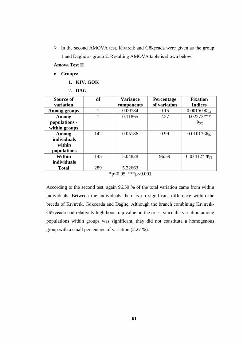
61
In the second AMOVA test, Kıvırcık and Gökçeada were given as the group
1 and Dağlıç as group 2. Resulting AMOVA table is shown below.
Amova Test II
Groups:
1. KIV, GOK
2. DAG
Source of
variation
df Variance
components
Percentage
of variation
Fixation
Indices
Among groups 1 0.00784 0.15 0.00150 ΦCT
Among
populations -
within groups
1 0.11865 2.27 0.02273***
ΦSC
Among
individuals
within
populations
142 0.05186 0.99 0.01017 ΦIS
Within
individuals
145 5.04828 96.59 0.03412* ΦIT
Total 289 5.22663
*p<0.05, ***p<0.001
According to the second test, again 96.59 % of the total variation came from within
individuals. Between the individuals there is no significant difference within the
breeds of Kıvırcık, Gökçeada and Dağlıç. Although the branch combining Kıvırcık-
Gökçeada had relatively high bootstrap value on the trees, since the variation among
populations within groups was significant, they did not constitute a homogenous
group with a small percentage of variation (2.27 %).

62
In the third AMOVA test, HemĢin and Çine Çaparı were joined as a group
and Herik was given as the other group. Resulting AMOVA table is shown
below.
Amova Test III
Groups:
1. HER
2. HEM, CIC
Source of
variation
df Variance
components
Percentage
of variation
Fixation
Indices
Among groups 1 -0.04495 -0.87 -0.00868***
ΦCT
Among
populations -
within groups
1 0.19212 3.71 0.03676***
ΦSC
Among
individuals
within
populations
134 0.12553 2.42 0.02494* ΦIS
Within
individuals
137 4.90876 94.74 0.05263***
ΦIT
Total 273 5.18145
*p<0.05, ***p<0.001
Again for this test, it can be observed that 94.74 % of the total variation came from
within individuals. But this time, there is a significant difference between individuals
within populations, means one of the breed is highly admixed. Also highly
significant minus value of fixation index of among groups implies that the groups
highly resemble each other in term of the variation of the individuals they contain.
This situation indicates Herik and the other two breeds had inter-migration in the
past. Lastly, although the branch combining Kıvırcık-Gökçeada had relatively high
bootstrap value on the trees, since the variation among populations within groups
was significant, again they did not constitute a homogenous group with a small
percentage of variation (3.71 %).

63
In the fourth AMOVA test, Sakız and Karagül are joined as a group and
Herik constituted the other group. Resulting AMOVA table is shown below.
Amova Test IV
Groups:
1. CIC
2. SAK, KRG
Source of
variation
df Variance
components
Percentage
of variation
Fixation
Indices
Among groups 1 0.04336 0.83 0.00828 ΦCT
Among
populations -
within groups
1 0.24397 4.66 0.04699***
ΦSC
Among
individuals
within
populations
136 -0.08040 -1.54 -0.01625 ΦIS
Within
individuals
139 5.02878 96.05 0.03952 ΦIT
Total 295 5.23571
***p<0.001
According to the results table, 96.05 % of the total variation came from within
individuals, but this time not significantly, means this time individuals are assigned
to the breeds better than those in other tests. The minus index of among individuals
within populations indicates the same result, as individuals resemble each other in
the breeds. Again the variation among populations within groups is significant,
implies that Sakız and Karagül are different in terms of genetic content, as asserted
from the tree results.

64
In the last AMOVA test, the dichotomous genetic structure of the breeds
observed in the tree was tested. Sakız, Karagül, HemĢin, Çine Çaparı, Norduz
and Herik were added in the first group and Karayaka, Dağlıç, Morkaraman,
Kıvırcık, Ġvesi, Gökçeada and Akkaraman were assigned to the second group.
Resulting AMOVA table is shown below.
Amova Test V
Groups:
1. SAK, KRG, HEM, CIC, NOR, HER
2. KRY, DAG, MOR, KIV, IVE, GOK, AKK
Source of
variation
df Variance
components
Percentage
of variation
Fixation
Indices
Among groups 1 0.10226 1.91 0.01908***
ΦCT
Among
populations -
within groups
11 0.19697 3.68 0.03747***
ΦSC
Among
individuals
within
populations
615 0.06046 1.13 0.01195* ΦIS
Within
individuals
628 5.00000 93.29 0.06711***
ΦIT
Total 1255 5.35969
*p<0.05, ***p<0.001
Among group variation found significant only in this test among the others. This
confirms the results of the trees that the breeds are split into two groups as one group
harboring the mainly the major ancient Turkish native sheep breeds and the other
group harboring relatively minor breeds.

65
3.2.3 „Individuals within Populations‟ Based Analyses
3.2.3.1 Factorial Correspondence Analysis (FCA)
The Factorial Correspondence Analysis (FCA) was used to visualize the individuals
in multidimensional space and to discover the relationships within and among the
breeds.
GENETIX v. 4. 05 (Belkhir et al. 1996–2004; http://univ-montp2.fr/~genetix) was
used for the analysis and the samples are inspected on 3-Dimensional graphics with
different triple combinations of first 4 factors (each represented by an axis) estimated
by the software. The results of the analysis are shown in Figure 3-8.
This graph shows us, although 19 (quite many) loci were studied; breeds are highly
overlapping and cannot be separated. Among all the breeds, samples of Ġvesi,
Karagül and Sakız to a certain degree; and Gökçeada, HemĢin and Çine Çaparı
(relatively) were observed to fall apart from the rest of the samples. Also, it can be
noticed that although Karagül and Sakız lie on the same side they are highly distinct.
They do not overlap, which confirms the idea that Sakız and Karagül are two highly
differentiated breeds. None of the breeds seem to have high inertia with non-
overlapping distribution with the distributions of other breeds, perhaps with the
exception of Sakiz. First three axes on FCA graphic exhibited 40,55% of the total
genetic variation.
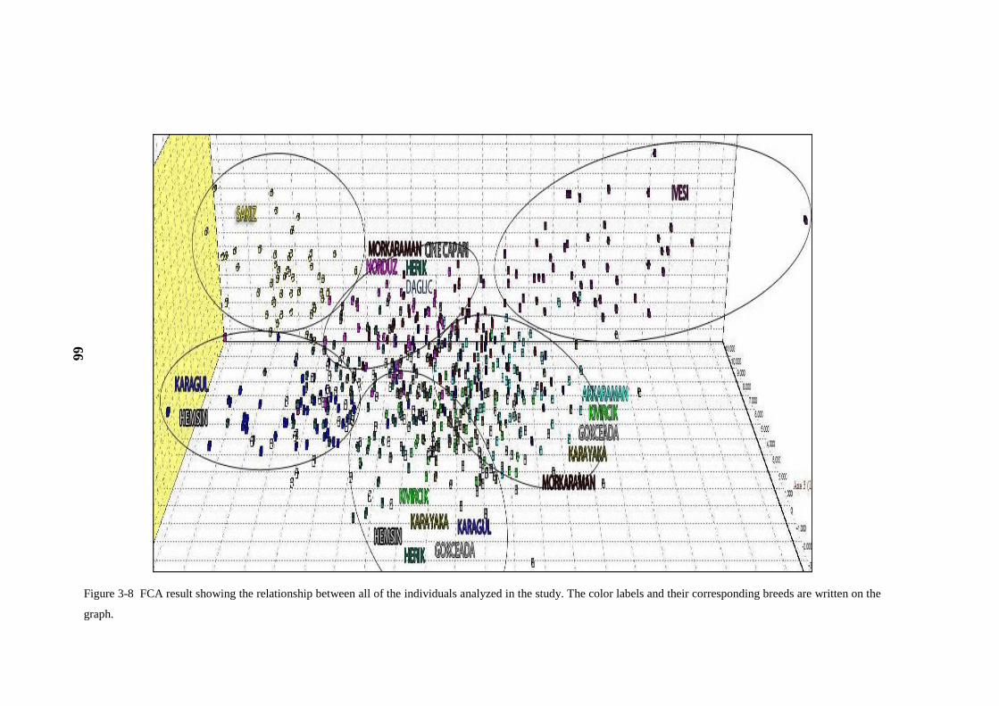
66
Figure 3-8 FCA result showing the relationship between all of the individuals analyzed in the study. The color labels and their corresponding breeds are written on the
graph.
66

67
3.2.3.2 Structure
The population structure and the level of admixture in the sheep breeds were
analyzed by using STRUCTURE v2.2.3 (Pritchard, et al. 2000) which is a model-
based clustering analysis.
Two different methods used to reveal the number of genetic clusters. According to
the method proposed by (Evanno, et al. 2005), at the true value of K, the second
order rate of change of the likelihood function (ΔK = m|L‟‟(K)|/ s[L(K)]) with
respect to K showed a clear peak. When this method was employed, most likely
number of partition in the dataset was found as K=10. The graph of the result of
calculations is given in the Figure 3-9.
Figure 3-9 The graph of the second order rate of change of the likelihood function
(ΔK = m|L‟‟(K)|/ s[L(K)]) with respect to K.
The graph showing the estimated population structures of the breeds is given in
Figure 3-10.

68
Figure 3-10 Structure Bar Plot based on the second order rate of change of the likelihood function when K=10, breed numbers and the breed names are given below
the graph. The abbreviations of the breeds are AKK for Akkaraman, CIC for Çine Çaparı, DAG for Dağlıç, GOK for Gökçeada, HEM for HemĢin, HER for Herik, IVE
for Ġvesi, KIV for Kıvırcık, KRG for Karagül, KRY for Karayaka, MRK for Morkaraman, NOR for Norduz and SAK for Sakız.
K = 10
68

69
At K=10, eight of the breeds were genetically distinct with relatively lower degree of
admixture: Sakız, Karagül, HemĢin, Çine Çaparı, Karayaka, Ġvesi, Gökçeada,
Akkaraman. Other breeds seemed to be admixed in various degrees. Despite the fact
that Sakız and Karagül were grouped in NJ tree (Figure 3-5, Figure 3-6, Figure 3-7)
in the structure, their distinctness from others as well as from each other were
evident. As was stated before, relatively long branch associated with Sakız and
Karagül emphasized that their similarity is only in their distinctness. Again
Gökçeada and Ġvesi had long branch lengths in the trees and they are distinct too.
Kıvırcık and Gökçeada constituted a group in all of the trees with relatively high
bootstrap values and then Dağlıç joined to them. This relationship can be observed as
the common genotype represented by dark blue color in the analysis. Among all of
the breeds the most admixed breed was Herik (had also the highest genetic diversity),
which confirms the results of the other tests, and then followed by Norduz, Dağlıç,
Morkaraman and Kıvırcık. Those breeds represented by short branch lengths in all
trees again were observed as being highly admixed. In the structure analysis some
degree of similarity between Dağlıç and Morkaraman was observed as the common
genotype represented by claret red color, which is further going to be discussed in the
next chapter of the thesis.
The approach which was employed in (Tapio, et al. 2010) study tests the similarity
between the results of individual runs for each different value of K. In the present
study at K=2, the similarity across 10 runs were high and consistent, but some
variable assignments for breeds was observed for other K values at different runs.
At K=2, as shown in the Figure 3-11 breeds were split with the same manner
observed in NJ trees into two broad groups as mainly major Turkish native sheep
breeds and the second group harboring relatively minor breeds.

70
Figure 3-11 Structure Bar Plot based on the when similarity between the results of individual runs for K=2, breed numbers and the breed names are given below the
graph. The abbreviations of the breeds are AKK for Akkaraman, CIC for Çine Çaparı, DAG for Dağlıç, GOK for Gökçeada, HEM for HemĢin, HER for Herik, IVE for
Ġvesi, KIV for Kıvırcık, KRG for Karagül, KRY for Karayaka, MRK for Morkaraman, NOR for Norduz and SAK for Sakız.
70

71
3.2.4 Genetic Barrier Estimation: Delaunay Network Analysis
Delaunay Network Analysis is conducted with the data obtained from the studied breeds
Based on Cavalli-Sforza and Edwards‟ chord distance, DC and Nei's DA genetic distance
with ENA corrections to construct the genetic barriers on map. Genetic barriers were
formed with thiessian triangles by shortest distance criteria. Figure 3-12 represents the
Delaunay Network Analysis formed with Cavalli-Sforza and Edwards‟ chord distance,
DC values and Figure 3-13 represents Delaunay Network Analysis formed with Nei's DA
genetic distance with ENA corrections values.
Figure 3-12 Delaunay Network by using Cavalli-Sforza and Edwards‟ chord distance,
DC values. Dots represent the locations of the sampling sites of the breeds. Black lines
are the constructed genetic barriers and numbers are the priority of the barriers near
them.
Priorities of the genetic barriers were as follows; the first five barriers separate one breed
at a time from the rest, as Sakız, Çine Çaparı, HemĢin, Ġvesi and Gökçeada, respectively.
Kıvırcık
Gökçeada
Sakız
Çine Çaparı
Dağlıç
Akkaraman
Karagül
Herik Karayaka
İvesi
Morkaraman
Hemşin
Norduz
1
2
3
4
5

72
Figure 3-13 Delaunay Network by using Nei's DA genetic distance with ENA corrections
values. Dots represent the locations of the sampling sites of the breeds. Black lines are
the constructed genetic barriers and numbers are the priority of the barriers near them.
Priorities of the genetic barriers were as follows; the first barrier separates Sakız from
the rest. Then the second barrier separates Çine Çaparı and Ġvesi at the same time, since
their distance from Akkaraman was equal. Third and fourth barriers separate HemĢin
and Gökçeada from the rest respectively.
Delaunay network analysis revealed that genetic barriers are isolating peripheral breeds,
as Sakiz being the most different one, from all the others. Kıvırcık, Dağlıç, Akkaraman,
Herik, Karayaka, Morkaraman and Norduz breeds are relatively more similar.
Kıvırcık
Gökçeada
Sakız
Çine Çaparı
Dağlıç
Akkaraman
Karagül
Herik Karayaka
İvesi
Morkaraman
Hemşin
Norduz
1
2
3
2
4

73
CHAPTER 4
DISCUSSION
In this part of the study, the results were reevaluated from different perspectives. First,
the interdisciplinary nature of the study was emphasized and the results were
summarized to compare with the results of comprehensive studies previously done on
sheep mainly in Europe. Some recommendations to obtain reliable microsatellite data
were made and possible implementations of the study for the development of
conservation strategies of the Turkish sheep breeds were discussed.
3.3 Interdisciplinary nature of the study; analyses and their complementary
contributions to the understanding of data.
This study presents a bioinformatics study covering a data based on 20 microsatellite
loci from 628 sheep representing 13 Turkish sheep breeds. Data collection was done as a
part of „In Vitro Conservation and Preliminary Molecular Identification of Some Turkish
Domestic Animal Genetic Resources-I‟ (TURKHAYGEN-I project). Molecular data
was collected by several students but author of the present study contributed the most.
Furthermore, outmost precautions were taken with the understanding that “If the data
was not reliable, then the results hence the conclusions would not be reliable”. First step
of data collection was the choice of the samples. Samples were chosen and collected by
the members of Ministry of Agriculture and Rural Affairs (MARA). They tried to
sample the sheep individuals from different flocks so that breed will not be represented
by the close relatives. Furthermore, their aim was to cover the whole span of the genetic
diversity of the breeds. However, because MARA members were well aware of the fact

74
that Turkish sheep breeds could be highly admixed, because ram exchanges between
flocks irrespective of their breeds is commonly experienced in Turkey, they tried to
avoid peripheral areas of the native distributions believing that in those areas individuals
would be mostly hybrids of the breeds. These were the cases for instance for Akkaraman
and Dağlıç samplings. In European countries sheep breeds were followed with their
herd-books and by the breed associations. As a result there is no hybridization between
the breeds, they are well isolated. Therefore, the problem of sampling an admixed
individual as a representative of the breed did not exist for a European breed. However,
in the samplings of this study, despite the efforts to avoid admixed individuals, there
were highly admixed individuals in many of the breeds as will be further discussed
below.
After sampling and receiving the bloods from 628 sheep individuals, biochemical -
molecular genetics methods were applied to amplify the 20 regions of genomes of the
domestic sheep. Molecular data in the form of genotypes of the individuals were
obtained. This stage was the starting point of Bioinformatics Avenue. Data was in the
form of peaks sent in the electronic form. They had to be converted into genotypes
expressed in numbers. Readings were done at least twice. To analyze the reliability of
the data, software tools (FreeNA, Arlequin, FSTAT) were used. With the help of these
software presence of null alleles and/or, possible incorrect readings for some of the loci
and possible sampling errors for the breeds (such as representing only close relatives
within a breed) were addressed. After gaining confidence in the data, further statistical
analyses were carried out, this time to understand the genetic diversity present within
and between breeds. The statistical methods were again embedded in software. Thereby,
capacity of the computers were used, calculations and significance tests that could not be
handled by ordinary calculators were done. As well as the software (for instance
FSTAT, 2001) some of the statistical methods (e.g. model-based clustering method
implemented in software STRUCTURE described in Pritchard, et al., 2000) themselves
were developed quite recently. During these analyses, to convert the data into input
format of each different tool, some scripts were written and used. Resulting statistics

75
were interpreted in accordance of the principles of population genetics and in the light of
historical background of the sheep breeds. Furthermore, obtained data were partly
standardized with international laboratories. With the new standardization efforts,
present data will be compatible with some of the previously generated data from other
laboratories. Hence, further analyses for wider geographic ranges will be made.
3.4 Revisiting the results of the present study
Out of 20 loci employed, except MAF214, 19 of them were found to be suitable for the
statistical analysis. In another recent study (Lawson Handley, et al., 2007) MAF214 was
not reported as a locus suffering from null alleles yet, deviations from expected
heterozygosities in that study is for MAF214 locus is noteworthy
To measure the overall diversity of breeds and locus one measure is the mean allelic
richness. The concept of allelic richness is well accepted as it is an allelic variation
measure robust to sample size and in the present study sample sizes of the breeds are
changing (40-51). For the 13 breeds, mean allelic richness based on the 19 loci was 9.79.
Allelic richness observed in the present study was considerably higher (7.87-9.81) than
those observed in Northern Eurasian sheep breeds (3.89-6.98) studied by Tapio et al.
(2010). The result confirms the expectation of high genetic diversity at the center of
domestication. Yet, this observation must be taken cautiously because employed loci in
two studies were different from each other. Allelic richness of the loci can give an idea
about the informativeness of the loci. If a new study using only 5 loci is going to be
started, since they posses the highest values perhaps INRA063, OarFCB304,
OarFCB226, OarFCB128 and DYMS1 loci should be preferred. However one must be
aware of the fact that these loci with high allelic richness may be giving the similar
information over and over again. When the components of FCA axes (these axes are
independent of each other and each tries to give the maximum genetic variability of the
data) were examined, in the first axes the most contributing loci were INRA63 and
OarFCB128. Whereas in the second axes, maximum genetic variability remained was

76
explained by INRA063, OarFCB226 and MAF33 the last locus is not among the ones
exhibiting highest allelic richness. Since, despite the fact that MAF33 has a moderate
allelic richness, it must have a unique contribution, after the aforementioned ones, in
describing the genetic diversity of the total data. Hence, allelic richness values describe
the value of the locus when each of them was considered individually. Heterozygosity
also reveals the within breed genetic diversities but this measure takes into account of
the frequencies of alleles as well as the number of alleles. Moreover expected
heterozygosity standardizes these frequencies in accordance with H-W equilibrium
principle, therefore, expected heterozygosity is the most commonly used measure to
describe the within group variation.
Considering expected heterozygosities, Karagül and Sakız breeds have the minimum,
while Kıvırcık, Karakaya and Dağlıç breeds have the maximum values. The factors such
as the level of admixture and the way of collecting the samples may have affected the
results. For example, Akkaraman was also expected to be among the ones with highest
heterozygosity values, since the breed is the one with highest population size. It is
probable that Akkaraman did not exhibit high diversity because a widespread sampling
could not be performed for Akkaraman.
Deviations from the Hardy-Weinberg equilibrium value (expected heterozygosities) did
not accumulate onto one of the loci or breeds, which increase the confidence of the
reliability of genotyping. HemĢin is the only breed with three loci exhibiting deviations
from Hardy- Weinberg equilibrium values. For other breeds total number of deviant loci
was two or less. Furthermore deviations in HemĢin were all due to excess of
homozygotes as would be expected for a population which is composed of isolated sub-
populations. Indeed, this can be a result from the geography of the North-East Anatolia
where the HemĢin breed is populated. In other words, the deviation in the three loci of
HemĢin breed is possibly due to the Wahlund effect.

77
The table of private alleles shows us there is only one allele 175 in OarJMP58 locus in
Gökçeada, an island breed, reaching to a significantly high frequency. Probably due to
isolation, either inbreeding frequency was increased or it could not spread to other
breeds raised in the Anatolia or Thrace. Other private alleles are low in frequency. Such
low frequencies imply that the breeds are admixed and there is no isolation between the
breeds.
Evaluation of the results based on allelic richness, Hardy-Weinberg equilibrium,
Linkage disequilibrium and FIS all indicated that data obtained based on 19 loci was not
giving any signal of error in genotyping the loci or in high degree of genetic relatedness
of the individuals within the total sample of the breed.
Although Wright has developed the very useful and informative F statistics in 1965,
usage of them was not common until recently, since the power of computation did not
allow making permutations to test the significance of this statistics. Genetic
differentiation among populations and among loci was evaluated by calculating locus-
specific and population pairwise FST‟s. The global estimate of FST (4%) which was quite
low compared to the 6–13% reported for European sheep breeds (Lawson Handley, et
al., 2007; Tapio, et al., 2010). Low degree of differentiation between the breeds was
expected due to the absence of isolation between the breeds. In spite of the absence of
isolation, pairwise FST values indicated that, all breeds are significantly genetically
differentiated. Ġvesi and Sakız breeds had particularly high values. These breeds may
harbor important uniquely adapted alleles and should, therefore, be given priority for
conservation.
It can be observed from the FIS table that HemĢin, Çine Çaparı, Morkaraman, Karayaka,
Ġvesi and Akkaraman have significant positive FIS values. Although, except HemĢin,
locus based deviations from Hardy-Weinberg proportions were not significant in these
breeds, apparently deviations of some loci were near to level of significance. Çine
Çaparı being started from few individuals must have small effective population size and

78
that may be the reason of having significant positive FIS value. But all of the others
Morkaraman, Karayaka, Ġvesi and as was already discussed Akkaraman, might be
indicating that these breeds were also exhibiting substructring and hence Wahlung
effects despite the presence of admixture. In another study conducted on the same breeds
with different samples (Koban et al., unpublished data) revealed significant positive FIS
values in the HemĢin, Morkaraman and Karayaka breeds indicating that observed
phenomenon was not due to sample specific but real and general.
When similarities between the breeds were searched by the trees constructed with the
help of different genetic distance measures, it was observed that trees generally
exhibited the same dichotomy pattern. Dichotomy implied that breeds are forming two
main genetically distinct groups. However, low bootstrap values (<60) on the nodes of
the trees indicated that the breeds were not well defined isolated distinct entities. On the
contrary they are composed of individuals which are overlapping genetically with a
considerable extend. The first group mainly composed of major Turkish native breeds
having relatively large area of distributions and large population sizes (Karayaka,
Dağlıç, Kıvırcık, Gökçeada, Akkaraman, Ġvesi, Morkaraman). In this group, two
geographically neighboring breed pairs Morkaraman-Norduz and Kıvırcık-Gökçeada
seemed to be relatively similar to each other. The second group of sheep breeds (Sakız,
Karagül, Norduz, Herik, HemĢin, Çine Çaparı) were either newly recovering from a
severe bottleneck (Çine Çaparı), or minor hybrid breed in the middle of major breeds
(Herik), newly introduced to Turkey from Turkmenistan (Karagül), significantly
composed by sub-populations –exhibiting Wahlund effect (HemĢin) and littoral breed
from the Aegean Coast (Sakız). Again within this group of breeds geographically
unrelated breed pairs Karagül-Sakız and HemĢin-Çine Çaparı seemed to be relatively
similar to each other. The groups consistently observed with relatively high bootstrap
values on the trees were further analyzed to reveal their homogeneity with AMOVA and
relatively higher (4.66% for Sakız-Karagül breeds and 3.71% for HemĢin-Çine Çaparı
breeds) but significant amount of variation was observed between each of them,
confirms the long branch lengths of them on the trees.

79
Other common groups observed on the trees (Morkaraman-Norduz and Kıvırcık-
Gökçeada) were also investigated by AMOVA. Again there was significant but
relatively smaller (3.20% Morkaraman-Norduz and 2.27% for Kıvırcık-Gökçeada
breeds) variations between the breed couples. In the literature (Aygün and Yılmaz, 2002;
Yılmaz and Cengiz, 2006) it is stated that Norduz is a variety of Akkaraman. Yet, in this
study and in the previous independent study Norduz seemed to be genetically more
related with Morkaraman. Perhaps the result is not surprising because they are two
neighboring breeds and in time admixture between them increased the genetic similarity
of these two breeds.
Another test of AMOVA conducted to check the dichotomous genetic structure observed
for all of the breeds in the trees. Indeed a small (1.91%) but significant variation was
observed between two groups as one group harboring the major ancient Turkish native
sheep breeds and the other group harboring relatively minor breeds.
Results of Factorial Correspondence Analysis exhibited that none of the breeds had high
inertia or was completely differentiated from the others. Yet, some of the breeds (Sakız,
Karagül and Ġvesi) were moderately differentiated, while Gökçeada, HemĢin and Çine
Çaparı were only relatively differentiated from the others. However, other breeds were
composed of the individuals highly overlapping with each other.
The results of the Delaunay Network Analysis was coherent with other analyses, by
indicating genetic barriers around Sakız, Gökçeada, Ġvesi, Çine Çaparı and HemĢin and
hence separating them from other breeds..
As revealed by the Bayesian cluster analysis (STRUCTURE), assuming that 13 breeds
were composed by the 10 independent populations (K=10), Sakiz, Karagül and Ġvesi
seemed to be relatively distinct and composed of relatively uniform individuals.
Furthermore, Gökçeada, HemĢin, Çine Çaparı and Akkaraman breeds have some amount

80
of admixed individuals but still their distinctness was visible. However, especially Herik
and Norduz seemed to be composed of highly admixed individuals.
3.5 Comparative evaluation of the results with those of the previous studies
One of the most comprehensive studies carried on sheep breeds was the one funded by
European Union in the context of Vth
Framework projects. The acronym was
ECONOGENE (Sustainable conservation of animal genetic resources in marginal rural
areas: integrating molecular genetics, socio-economics and geostatistical approaches). In
ECONOGENE genetic diversity and subdivision of 57 European and Middle-Eastern
sheep breeds in terms of 31 microsatellite markers were investigated. Four Turkish
sheep breeds (Dağlıç, Akkaraman, Morkaraman and Karayaka) were also studied in that
project. For those 4 breeds common in both of the studies (ECONOGENE and present),
the samples were independently collected.
One major result of the ECONOGENE project was the presence of a genetic barrier
(Peter, et al., 2007) between the European and Middle Eastern (breeds from Saudi
Arabia, Egypt and Cyprus) sheep breeds. This barrier was going through the Anatolia
between Akkaraman and Dağlıç, the two neighboring breeds in the absence of major
geographic or political barriers. This result was puzzling because it was a well known
fact that rams have been exchanged between the breeds, especially more frequently
between the neighboring breeds. Presence of genetic barrier was interpreted as the
consequence of migration of sheep from the Central and Eastern Asia to Turkey. It was
argued that heavy mixture was in Akkaraman and in those breeds which are on the east
of Akkaraman. In the present study less number of loci (31 vs. 19) were used and 9 out
of 13 breeds examined were different and all of them were from Turkey where genetic
exchange between the breeds was allowed and quite common. Here, this barrier was
absent (results of Delaunay, trees and FCA). However, the same barrier could be seen
in the mtDNA haplogroup data based analysis for the same individuals

81
(TÜRKHAYGEN-I, 7th
interim report) as the 4th
genetic barrier in Delaunay analysis.
Perhaps, since the samples of Dağlıç and Akkaraman chosen for this study are different
than those of the previous study, they exhibited different between breed relationships.
These results suggest that observation of a between breed relation very much depends on
the samples and the breeds considered.
Dağlıç in the present study was genetically close to Morkaraman-Norduz pair (FST and
STRUCTURE). Information collected from local farmers indicated that Morkaraman
individuals were brought to the area, previously, where Dağlıç samples were collected
for the present study. Since Morkaraman individuals were not in the area by the time of
Dağlıç sample collection, local farmers never mentioned the previous presence of
Morkaraman individuals. Only when they were explaining how an allergic reaction of
Dağlıç to a plant was avoided by bringing Morkaraman individuals, the link between
Dağlıç and Morkaraman was explained. The anecdote confirmed genetic admixture and
increased the confidence to the data and results.
In one previous study (Koban, 2004) based on 5 microsatellite loci, high degree of
differentiation between the state farm samples of Akkaraman breed with that of
collected from local farmers was presented. This provided the strong evidence for the
need of sampling of the breed as few individuals from many different flocks. It was seen
that if many flocks, preferably distant flocks, were not sampled, breed may not be
represented appropriately.
In another study involving five Turkish native sheep breeds (excluding the Western
breeds) 30 microsatellite were used where three of them were common with those of the
present study (Uzun et al, 2006). The main conclusion was that fat tailed breeds were
different from those of the thin tailed breeds. In the present study, as well as in
ECONOGENE no such conclusion could be drawn. In this case, importance of sampled
breeds and sampling in drawing conclusions was seen once more.

82
There were some other studies carried out on sheep in Turkey in the early days of
microsatellite studies (Bulut et al., 2004; Soysal et al., 2005). However, those studies
involved few (3-5) loci and few breeds and were addressing the relatedness of hybrid
breeds with their parents.
Present study covers the analysis of all loci and all breeds which were targeted in
TURKHAYGEN-I project. Before the final stage of the studies in February 2009 an
analysis was carried out with 7 breeds and 14 or fewer loci (Doğan, 2009). Data of the
previous study has been modified considerably and results of it were extended in this
present study.
In a recent large scale study done by Tapio et al. (2010) well differentiation between the
three groups of sheep (termed as Nordic, Composite and Fat-tailed) from the Eurasian
subcontinent with 20 microsatellite markers was reported. Generally in Europe well
differentiation of the breeds was observed as was seen, for instance, from Tapio et al.‟s
(2010) study in (Figure 4-1). However, as was seen from the results of present study,
highly admixed Turkish breeds did not give such clear distinctness generally.

83
Figure 4-1 STRUCTURE Analyses for the Breeds from Northern Eurasia. Individuals
are presented as vertical lines divided into K colors, representing constructed
populations, breeds descending mainly from the northernmost edge of the Europe are
divided into 7 sub-clusters. Taken from Tapio et al. (2010).
3.6 Recommendations in relation to Genotyping based on microsatellite loci
First of all, it was experienced that, low DNA quality can seriously diminish the
consistency of the data. Therefore DNA isolation step should be done carefully and all
the chemicals used should be fresh and sterile. During wet lab experiments, extreme
cautions should be taken in optimization of the Polymerase Chain Reactions (PCR)
amplification and in each application of the procedure. Small changes in concentration
of DNA and other chemicals can change the amplification of some specific alleles as
was also reported previously (Hoffman, 2005; Goossens, et al., 1998). Genotyping

84
errors can also occur due to the preferential amplification of small alleles (i.e. large
allele dropout or short allele dominance, Wattier, et al., 1998), deviations from a regular
repeat motif (suggesting indels) and stuttering (failure to discriminate similar sized
alleles in genotypes due to PCR artifacts). Hence, before genotyping microsatellite
alleles from the output “.fsa” folders containing raw data coming from ABI310 fragment
analyzer, a significant expertise should be gained by the researcher and each locus
should be read only by one person to be consistent in allele calling. Furthermore, the
reliability of the resulting genotypes must be verified by independent readings of the
same person.
After obtaining genotypic data of the samples, the data should be analyzed in a statistical
software tool to extract the allele frequency of the data. Examinations of allele
frequencies by the specially developed tools would indicate if there is an inconsistency
in the naming the same alleles in different breeds. There are a variety of tools developed
for this purpose. Just like the problem with many sequence formats, each of these tools
has its own data format. As a result, there is a significant demand for a program to
convert the data formats easily. In this study several such programs had been written as
small scripts which are reading data from text files and writing it into another with a
required format (given in Appendix E). However, during many sequential and
demanding analyses, after a while, all of these converted data start to accumulate into a
huge data, occupying significant amount of computer memory. Therefore, programs
must be unified such that they will all be able to process and produce the same data
format.
Analyzing allele frequency at the first sight would give some information about the
genotyping quality. For example, alleles should be named according to the type of the
microsatellite (in terms of repeating unit length). If it is a two base repeating locus, most
of the alleles should be named as even or odd numbers (like 112, 114, 116…). It should
be kept in mind that again some exceptions are present in this case. If there is an indel,
the alleles start to change their all even or all odd features. This can be analyzed by

85
opening the raw data (electropherograms) of the suspected samples together with the
superimposed size marker peaks. It must be remembered that, alleles with an extremely
low frequency could be either misreading as well as private alleles.
Along with testing the reliability of the genotyping, there was a great discrepancy
between the number of alleles observed by the ECONOGENE and those of the present
study for the locus MAF214. Potential reasons for this difference could be genotyping
error. The suggested range of locus MAF214 is 186-204 in literature. This range may
change according to the data (the breeds studied could be more divergent or there could
be a region specific mutation for that locus which could increase or decrease the range of
it). Usually every allele of a locus looks similar to each other which help to the
researcher in identifying non-specific bands. However, there are some exceptional
phenomena for some microsatellite loci; as was already mentioned in the present
manuscript, one of them is known as short allele dominance or large allele drop-out
(Wattier, et al., 1998). It is the preferential amplification of shorter alleles and can result
in a significant heterozygote deficiency. For the locus MAF214, this case was observed
and distinguishing alleles from the non-specific bands became difficult. As a result, it
was decided that only the alleles in the suggested range were considered and this most
probably caused a deviation in the number of alleles between the two studies. In
ECONOGENE project, for the MAF214 locus, there were 41 alleles, very high number
implying high risk of making an error. However, 6 alleles observed in the present study
perhaps were very low because analysis indicated that there were too many null alleles.
Therefore, it was considered as neither the ones observed by the ECONOGENE nor the
ones observed in the present were reliable to be included in further analysis.
When the template DNA is damaged or there are some mutations at the annealing site of
the primer, null alleles occur. As well as detecting null alleles by FreeNA software, one
can make use of the fact that null alleles have their own specific allelic features, like
deficiencies and excesses of particular genotypes in relatively few loci. Hence,
86
deviations due to the various genotyping errors can be distinguished from those caused
by nonpanmixia. (Cock Van, et al., 2004)
In a previous study of Lawson Handley (2007), 29 European sheep breeds were
investigated with 23 microsatellite loci, and high amount of null alleles were obtained.
To eliminate the misleading effects of null alleles, FreeNA software was used and it was
supposed that values of r < 0.20 are not expected to cause significant problems in
analyses; therefore, only loci with r ≥ 0.20 were considered to be potentially problematic
for the calculations. In the 2007 paper on FreeNA software, Chapuis et al. were grouped
the loci into three classes of null allele frequency: negligible (r < 0.05), moderate (0.05 ≤
r < 0.20) or large (r ≥ 0.20). In this study, to be more conservative, r ≥ 0.05 was taken as
the threshold for null allele frequency.
Incidentally, ISAG (International Society for Animal Genetics) and FAO (Food and
Agriculture Organization) recommend a list of highly polymorphic and informative
microsatellite loci to prevent scientists from wasting their time and money. All 20 loci
were selected from this list. Probably, the conflict in relation to MAF214 after being
reported by the present study will cause the exclusion of the locus from the list. Another
reason of choosing markers from the recommended list was to produce data in the line of
previous reports and check the generality of the observed results. For instance, in a
spatial analysis to find out the association of microsatellites with the changing
geographic or physical environmental conditions an analysis in sheep was carried out
(SAM analysis software, Joost, et al., 2008). Since microsatellites were in general
considered as neutral loci, no association was the null expectation. Yet, if there was an
association this would indicate the linkage of the locus to a gene which was selected by
the condition. In that study, there was an association between the environmental
parameters such as precipitation and the alleles of OarFCB304 and DYMS1 loci. When
the OarFCB304 locus was subjected to SAM test with the data of present study, the
same association was observed with a high significance (TÜRKHAYGEN-I 5th
and 6th
interim report). Other locus was not subjected to the same test yet.

87
To standardize the data from different countries and breeds every year, ISAG sends a
small number of samples to the laboratories working with microsatellites all around the
world to be run and genotyped in the same manner. In this way all the accredited
laboratories would call the same allele with the same name and all the data become
standardized. This enables our data to be added into database of microsatellite genotypes
for further world-wide genetic variation and population structure analyses. For our test
results, if we genotype our data again by using ISAG standardized allele names, means
get rid of the systematic errors caused by only allele names, our data, before the second
reading of the whole data, was calculated to be 80% reliable. To improve this reliability
we started to use an upgraded model of the sequencer (Applied Biosystems - ABI3100),
by which high quality raw data was obtained. Yet, it requires new primers with different
fluorescent labels. Therefore, analysis of only six of the twenty microsatellite loci could
be repeated with this new machine.
3.7 Possible implementations of the results
Archaeological (Zeder, 2008) and genetic (Hiendleder, et al., 1998, 2002; Pedrosa, et
al., 2005; Bruford and Towsend, 2006) evidences indicated that sheep was domesticated
in the region from Central Anatolia to North Zagros Mountains about 11000 years ago.
In the next 5000 years along with the agro-pastoralism domestic sheep went to West and
North Europe (Price, 2000), Central Asia (Harris, 1996) and North Africa (Barker,
2002). In accordance with the presented evolutionary history of sheep, Turkish native
sheep might be the closest descendents of the ancestral domestic sheep. Although with
respect to production parameters, Turkish native sheep breeds were inferior to Western
European breeds such as Merino sheep, their ability to survive at the extreme
environmental conditions (extreme temperatures, low food quality) and resistance to
parasites indicated that they may be the reservoirs of special alleles and that they may
help to humanity in the future upon changing environmental conditions. Indeed,

88
generally high genetic diversity observed in the Middle Eastern region (Peter, et al.,
2007; Lawson Handley, et al., 2007) was taken as a support for the presence of high
genetic diversity in the Middle Eastern sheep breeds. Again this diversity must be
maintained as wealth that will enable sheep to survive in changing environmental
conditions. On the other hand crises of loss of diversity in the world (FAO, 2006) and
also in Turkey (Kaymakçı et al., 2000; Ertuğrul et al., 2000) call an urgent need of
sound conservation plans in Turkey. With the help of cryo-conservation practices only
limited amount of genetic material can be conserved. Furthermore, since they are not in
contact with the natural selection, in the long run they may not be able to survive under
the new environmental conditions. It is best to conserve the breeds within their changing
environments. It is obvious that not all of the Turkish breeds can be conserved. Perhaps
among the ones which are at high risk of hybridization with economically important
ones or the rare ones or the ones exhibiting high and unique combinations can be given
priority. Yet, decisions towards prioritization need extensive and reliable genetic data
and comparative analyses. Present study, provides a background for the decision makers
in deciding about the breed(s), which will have priority in conservation studies. Yet, in
conservation studies there is no unique recipe. In one approach maximum genetic
diversity is tried to be maintained with minimum number of conserved breeds (Caballero
and Toro, 2002). However, it is also known that conservation of unique genetic diversity
is of great value (Glowatski et al. 2009). Distinct breeds with unique diversity may not
exhibit high genetic diversity. For instance, based on allelic richness Herik seemed to be
the richest. However, observing Herik in STRUCTURE analysis, as a breed composed
of individuals which are all highly admixed, one can realize that allelic richness of Herik
is high only because it is admixed. It may not hold any unique alleles; on the contrary it
may have lost the locally co-adapted gene complexes during the admixture. Whereas
Ġvesi, both having high genetic diversity and exhibiting distinct and unique gene pool
(represented by one color in STRUCTURE, and secondly separated in Delaunay drawn
with Nei's DA genetic distance with ENA corrections values) may have high priority in
conservation studies. Similarly, Sakız with its highly distinct gene pool and high twin
rate may deserve priority in conservation. The breeds within Anatolia and combining in

89
“the mainly major breeds” group are relatively less distinct. Among those, Akkaraman
and Morkaraman are not endangered due to their rather high population sizes. Therefore,
Dağlıç and Karayaka among these main breeds, may have priority in conservation
because they are known to have local adaptation (Dağlıç, because of its special mouth
structure can graze over the stony hills whereas Karayaka, since it has such a wool
structure that rain can not penetrate inside its pelt) and furthermore Dağlıç is heavily
threatened with thin tailed breeds and Karayaka is low in number. However, since the
results seemed to depend on sampled breeds and samples, it is recommended that before
the action similar study with new independent collected samples must be carried out.
Another comment about the conservation of peripheral and distinct breeds is as follows:
These are distinct with respect to major native breeds in Anatolia, yet may not be
distinct with respect to the breeds of neighboring countries, such those in Syria, Georgia
and Greece. It would be interesting to carry out studies similar to the present study in
those countries and examine these trans-boundary breeds to establish a cooperative
strategy for the conservation of these breeds. Therefore, with the help of these suggested
studies more sound and economical strategies may emerge in the context of diversity
conservation in sheep species.
Furthermore, the genetic data and analyses may also help in deciding which individuals
of the breed should be conserved. When one has an extensive data from sheep, as was
the case for the present study and relying on the results of comparative studies such as
the results of STRUCTURE, individuals of a breed can be judged if they were admixed
and if found to be so it can be purged from the flocks which are going to be conserved.
In Faroe Island there were cattle and it was known that in early days there was an
indigenous breed. However, the native individuals were crossed with Norwegian cattle
breeds to improve the productivity. A population genetics study conducted on the breeds
in neighboring mainland, Norwegian cattle and almost all of the individuals of native
breed with 20 microsatellite loci by using fundamental biostatistics methods such as

90
FCA and STRUCTURE (Li, et al., 2005). The results indicated that out of 40 native
individuals only six of them were relatively free of admixture and the indigenous breed
using only these six individuals can be recovered. Recently Çine Çaparı went through a
recovery process. If there were genetic data the most suitable individuals for the Çine
Çaparı recovery could have been selected in the same manner.
Results of the present study together with the experiences gained by the team of young
researchers are expected to contribute to the conservation of sheep genetic diversity as
well as to the conservation of animal diversity studies in general.

91
CHAPTER 5
CONCLUSION
1) By the present study molecular genetic diversity for 13 sheep breeds of Turkey
(Sakız, Karagül, HemĢin, Çine Çaparı, Norduz, Herik, Dağlıç, Morkaraman,
Kıvırcık, Karayaka, Ġvesi, Gökçeada and Akkaraman), based on 20 microsatellite
loci, was determined and analyzed.
2) Through the study an experience was gained, by a team of researchers in
collecting a reliable microsatellite based data.
3) It is realized that with the STRUCTURE analysis, admixture history of the
breeds can be traced as it was for Dağlıç breed.
4) On the contrary of belief it is observed that, Norduz is closely related with
Morkaraman.
5) It is concluded that Turkish breeds are significantly different from each other, all
of them exhibit high within group genetic diversity and they are admixed to a
various degrees.
6) In general peripheral breeds (Gökçeada, Sakız, Çine Çaparı, Ġvesi, HemĢin and
Karagül) are distinct from the others.
7) Breeds in and around Central Anatolia, although they are significantly different
from each other (Karayaka, Dağlıç, Herik, Akkaraman, Morkaraman, Norduz

92
and Kıvırcık) seemed to have no detectable- significant genetic barriers between
them.
8) Data and results of the present study can be used in deciding the conservation
priorities of the breeds. It is suggested that: Sakız, Ġvesi, Dağlıç, Karayaka must
have high priority in conservation.
9) However, it must be emphasized that samples and studied breeds may affect the
observed patterns of genetic diversity. Hence, an independent study must be
carried out before the major steps in conservation of sheep breeds will be taken.
10) The most importantly, it is seen that results of the present study can be used in
formation and management of the conservation flocks.

93
REFERENCES
Allendorf, F. W. 1986. Genetic drift and the loss of alleles versus heterozygosity. Zoo
Biology 5(2):181-190.
Allendorf, F. W., and G. Luikart 2007. Conservation and the Genetics of Populations.
First Edition, Wiley-Blackwell, MA, USA.
Ammerman, A. J., and L. L. Cavalli-Sforza 1973. A Population Model for the Diffusion
of Early Farming in Europe. The Explanation of Culture Change 343-57.
Aygun T., Yilmaz A. 2002, Akkaraman Varyetesi Norduz ve KarakaĢ Erkek Kuzularının
Bazı Testis Özellikleri Bakımından KarĢılaĢtırılması, YYÜ Veterinerlik Fakültesi
Dergisi, Vol 13, pp. 12-14.
Barbujani, G., A. Pilastro, S. De Domenico, and C. Renfrew 1994. Genetic variation in
North Africa and Eurasia: Neolithic demic diffusion vs. paleolithic colonisation.
American Journal of Physical Anthropology 95(2):137-154.
Barker, G 2002. In: Bellwood, P., Renfrew, C., (eds) Examining the Farming/Language
Dispersal Hypothesis. The McDonald Institute Monographs, Cambridge, pp. 151–162.
Beaumont, Mark A., and Bruce Rannala 2004. The Bayesian revolution in genetics. Nat
Rev Genet 5(4):251-261.
Belkhir, K., Borsa, P., Chikhi L., Raufaste, N., and Bonhomme, F 1996–2004.
GENETIX 4.05, logiciel sous Windows pour la ge´ne´tique des populations. Universite´
de Montpellier II, Montpellier, France.
Bernardo C., Pereira F., Arnaud F. 2009, Revealing the History of Sheep Domestication
Using Retrovirus Integrations, Science, Vol 324, pp. 532-536.

94
Bulut, Z., Nizamlıoğlu, M. and Togan, I. 2004. Analysis of the genetic structure of
native and crossbreed sheep breeds with microsatellite markers. II. National Veterinary
Biochemistry and Clinic Biochemistry Congress, Elazığ, Turkey.
Botstein, D., White R.L., Skolnick, M., and Davis, R.W 1980. Construction of a genetic
linkage map in man using restriction fragment length polymorphisms. Am J Hum Genet
32(3):14–331.
Bowcock, A. M., A. Ruiz-Linares, J. Tomfohrde, E. Minch, J. R. Kidd, and L. L.
Cavalli-Sforza 1994. High resolution of human evolutionary trees with polymorphic
microsatellites. Nature 368(6470):455-457.
Brassel, K. E., and D. Reif 1979. A procedure to generate thiessian polygons.
Geographical Analysis 11: 289-303.
Brinkmann, Bernd, Michael Klintschar, Franz Neuhuber, Julia Hühne, and Burkhard
Rolf 1998. Mutation Rate in Human Microsatellites: Influence of the Structure and
Length of the Tandem Repeat. American journal of human genetics 62(6):1408-1415.
Brookfield, J. F. Y. 1996. A simple new method for estimating null allele frequency
from heterozygote deficiency. Molecular Ecology 5(3):453-455.
Bruford M.W., Townsend S.J. 2006, Mitochondrial DNA diversity in modern sheep:
Implications for domestication. In: Zeder M.A., Bradley D.G., Emshwiller E., Smith
B.D. (Eds.) Documenting Domestication: New Genetic and Archaeological Paradigms.
University of California Press, CA,USA, 307-317.
Bruford, Michael W., Daniel G. Bradley, and Gordon Luikart 2003. DNA markers
reveal the complexity of livestock domestication. Nat Rev Genet 4(11):900-910.
Caballero A., Toro M.A. 2002. Analysis of genetic diversity for the management of
conserved subdivided populations. Conserv. Gen., (3), 289–299.

95
Cavalli-Sforza, L. L., and A. W. Edwards 1967. Phylogenetic analysis. Models and
estimation procedures. American journal of human genetics 19(3 Pt 1):233-57.
Chakraborty, R., M. D. Andrade, S. P. Daiger, and B. Budowle 1992. Apparent
heterozygote deficiencies observed in DNA typing data and their implications in
forensic applications. Annals of Human Genetics 56(1):45-57.
Chakraborty, Ranajit, Marek Kimmel, David N. Stivers, Leslea J. Davison, and Ranjan
Deka 1997. Relative mutation rates at di-, tri-, and tetranucleotide microsatellite loci.
Proceedings of the National Academy of Sciences of the United States of America
94(3):1041-1046.
Chapuis, Marie-Pierre, and Arnaud Estoup 2007. Microsatellite Null Alleles and
Estimation of Population Differentiation. Mol Biol Evol 24(3):621-631.
Chikhi, Lounès, Richard A. Nichols, Guido Barbujani, and Mark A. Beaumont 2002. Y
genetic data support the Neolithic demic diffusion model. Proceedings of the National
Academy of Sciences of the United States of America 99(17):11008-11013.
Cock Van, Oosterhout, Hutchinson William F, Wills Derek P. M, and Shipley Peter
2004. micro-checker: software for identifying and correcting genotyping errors in
microsatellite data. Molecular Ecology Notes 4:535-538.
DAD-IS 2010. Domestic Animal Diversity Information System (DAD-IS),
Dempster, A. P., N. M. Laird, and D. B. Rubin 1977. Maximum Likelihood from
Incomplete Data via the EM Algorithm. Journal of the Royal Statistical Society. Series
B (Methodological) 39(1):1-38.
Doğan A.ġ. 2009, Reassessment of Genetic Diversity in Native Turkish Sheep Breeds
with Large Numbers of Microsatellite Markers and Mitochondrial DNA (MTDNA),
Master Thesis, Biology Department, Middle East Technical University, Ankara, Turkey.
Drury, Douglas W., Ashley L. Siniard, and Michael J. Wade 2009. Genetic
Differentiation among Wild Populations of Tribolium castaneum Estimated Using
Microsatellite Markers. J Hered:esp077.

96
Edwards, Al, Holly A. Hammond, Li Jin, C. Thomas Caskey, and Ranajit Chakraborty
1992. Genetic variation at five trimeric and tetrameric tandem repeat loci in four human
population groups. Genomics 12(2):241-253.
Erol H. and Akçadağ H. Ġ. 2009 Some production characteristics of Karagül sheep on
insitu conditions. Lalahan Hayvan Arastırmaları Enstitüsü Dergisi 49(2):91-104.
Ertuğrul, M., N. Akman, G. Dellal, T. Goncagül 2000. Hayvan Gen Kaynaklarının
Korunması ve Türkiye Hayvan Gen Kaynakları. Türkiye Ziraat Mühendisliği V. Teknik
Kongresi (2 cilt) Yayın No:38, Ankara.
Evanno, G., S. Regnaut, and J. Goudet 2005. Detecting the number of clusters of
individuals using the softwarestructure: a simulation study. Molecular Ecology 14:2611-
2620.
Excoffier, L., G. Laval, S. Schneider 2006 ARLEQUIN version 3.01: an integrated
software package for population genetics data analysis. University of Bern, Institute of
Zoology, Switzerland. Available from http://cmpg.unibe.ch/software/arlequin3
Excoffier, L., P. E. Smouse, and J. M. Quattro 1992. Analysis of Molecular Variance
Inferred From Metric Distances Among DNA Haplotypes: Application to Human
Mitochondrial DNA Restriction Data. Genetics 131(2):479-491.
Falush, Daniel, Matthew Stephens, and Jonathan K. Pritchard 2003. Inference of
Population Structure Using Multilocus Genotype Data: Linked Loci and Correlated
Allele Frequencies. Genetics 164(4):1567-1587.
Falush, Daniel, Matthew Stephens, and Jonathan K. Pritchard 2007. Inference of
population structure using multilocus genotype data: dominant markers and null alleles.
Molecular Ecology Notes 7(4):574-578.
FAO, 2004. Food and Agriculture Organization of United Nations (2004) – Secondary
guidelines for development of national farm animal genetic resources management
plans: measurement of domestic animal genetic diversity (MoDAD): Recommended
microsatellite markers, Rome, Italy

97
FAO 2006. Animal genetic resources – time to worry? Irene Hoffmann and Beate
Scherf, Livestock Report, http://www.fao.org/docrep/009/a0255e/a0255e00.HTM
Food and Agriculture Organization of the United Nations. <http://www.fao.org/dadis/>
Last viewed 10 September 2010.
Francisco, L., A. Langsten, C. Mellersh, C. Neal, and E. Ostrander 1996. A class of
highly polymorphic tetranucleotide repeats for canine genetic mapping. Mammalian
Genome 7(5):359-362.
Glowatzki-Mullis M.-L., Muntwyler J., Baumle E., Gaillard C. 2009, Genetic diversity
of Swiss sheep breeds in the focus of conservation research, J. Anim. Breed. Genet.,
Vol. 126, pp. 164-175.
Goldstein, D. B., and C. Schlötterer 2000. Microsatellites: evolution and applications.
Oxford University Press, London.
Goossens, B., L. P. Waits, and P. Taberlet 1998. Plucked hair samples as a source of
DNA: reliability of dinucleotide microsatellite genotyping. Molecular Ecology
7(9):1237-1241.
Gorman, George C., and Joseph Renzi, Jr. 1979. Genetic Distance and Heterozygosity
Estimates in Electrophoretic Studies: Effects of Sample Size. Copeia 1979(2):242-249.
Goudet, J 2001. FSTAT, a program to estimate and test gene diversities and fixation
indices (version 2.9.3). Available from http://www.unil.ch/izea/softwares/fstat.html .
Updated from Goudet (1995) http://www2.unil.ch/popgen/softwares/fstat.htm)
Harris D. R., C. Gosden 1996. In: Harris, D., (eds) The Origins and Spread in
Agriculture and Pastoralism in Eurasia, UCL Press, London, pp. 370–389.
Hiendleder S., Mainz K., Plante Y., Lewalski H. 1998, Analysis of mitochondrial DNA
indicates that domestic sheep are derived from two different maternal sources: No
evidence for contributions from Urial and Argali sheep. Journal of Heredity, 89:113-
120.

98
Hiendleder S., Kaupe B., Wassmuth R., Janke A. 2002, Molecular Analysis of Wild and
Domestic Sheep Questions Current Nomenclature and Provides Evidence for
Domestication from Two Different Subspecies. Proc. R. Soc. Lond. B 269, 893-904.
Hoffman JI., Amos W. (2005), Microsatellite genotyping errors: detection approaches,
common sources and consequences for paternal exclusion, Molecular Ecology, Vol 14,
pp. 599–612.
Hoffman, J. I., and W. Amos 2005. Microsatellite genotyping errors: detection
approaches, common sources and consequences for paternal exclusion. Molecular
Ecology 14(2):599-612.
Jobling, M. A., M. E. Hurles, and C. Tyler-Smith 2004. Human Evolutionary Genetics:
origins, peoples and disease. London/New York: Garland Science Publishing, 523 pp.
Joost, S., M. Kalbermatten, and A. Bonin 2008. Spatial analysis method (sam): a
software tool combining molecular and environmental data to identify candidate loci for
selection. Molecular Ecology Resources 8(5):957-960.
Kaymakçı, M., A. Eliçin, E.Tuncel , E. Pekel, O. Karaca , F. IĢın, T. TaĢkın, Y. AĢkın,
H. Emsen, M. Özder, E. Selçuk, R. Sönmez 2000. Türkiye‟de KüçükbaĢ Hayvan
YetiĢtiriciliği. Türkiye Ziraat Mühendisliği V. Teknik Kongresi, 17-21 Ocak 2000,
Ankara
Koban, E 2004. Genetic Diversity of Native and Crossbreed Sheep Breeds in Anatolia.
PhD Thesis. Middle East Technical University, Ankara, Turkey.
Koban, E., Perez, T., Bruford, M. W., Togan, Ġ. 2010. A Genetic Analysis of Marginal
Sheep Breeds From Turkey. Submitted manuscript.
Langella, M 1999. Populations 1.2.30: Population genetic software (individuals or
population distances, phylogenetic
trees).http://bioinformatics.org/~tryphon/populations/. Accessed 10 Mar 2009.

99
Lawson Handley, L. J., K. Byrne, F. Santucci, S. Townsend, M. Taylor, M. W. Bruford,
and G. M. Hewitt 2007. Genetic structure of European sheep breeds. Heredity
99(6):620-631.
Lebart, L ; Morineau, A; Warwick, K M 1984. Multivariate descriptive analysis:
Correspondence analysis and related techniques for large matrices. .304 pp.
Lewontin, R. C. and K. Kojima 1960, The evolutionary dynamics of complex
polymorphisms, Evolution Vol. 14, pp. 458-472.
Li, M., K. Sternbauer, P. Haahr, and J. Kantanen 2005. Genetic components in
contemporary Faroe Islands Cattle as revealed by microsatellite analysis. Journal of
Animal Breeding and Genetics 122(5):309-317.
Lowe1 W., Allendorf F. 2010, What can genetics tell us about population connectivity?
Molecular Ecology, Volume 19, Issue 15, pages 3038–3051.
Luikart, Gordon, and Phillip R. England 1999. Statistical analysis of microsatellite DNA
data. Trends in Ecology & Evolution 14(7):253-256.
Machugh, David E., Ronan T. Loftus, Daniel G. Bradley, Paul M. Sharp, and Patrick
Cunningham 1994. Microsatellite DNA Variation within and among European Cattle
Breeds. Proceedings: Biological Sciences 256(1345):25-31.
Meadows J.R.S., Cemal I., Karaca O., Gootwine E., Kijas J.W. 2007, Five ovine
mitochondrial lineages identified from sheep breeds of the Near East. Genetic,.
175:1371-1379.
Meadows, J. R. S., K. Li, J. Kantanen, M. Tapio, W. Sipos, V. Pardeshi, V. Gupta, J. H.
Calvo, V. Whan, B. Norris, and J. W. Kijas 2005. Mitochondrial Sequence Reveals High
Levels of Gene Flow Between Breeds of Domestic Sheep from Asia and Europe. Journal
of Heredity 96(5):494-501.
Mellersh, Cathryn S., Amelia A. Langston, Gregory M. Acland, Melissa A. Fleming,
Kunal Ray, Neil A. Wiegand, Leigh V. Francisco, Mark Gibbs, Gustavo D. Aguirre, and
100
Elaine A. Ostrander 1997. A Linkage Map of the Canine Genome. Genomics 46(3):326-
336.
Monmonier, M 1973. Maximum-difference barriers: An alternative numerical
regionalization method. Geographical Analysis 3: 245-261.
Mousadik, A., and R. J. Petit 1996. High level of genetic differentiation for allelic
richness among populations of the argan tree [Argania spinosa (L.) Skeels] endemic to
Morocco. TAG Theoretical and Applied Genetics 92(7):832-839.
Naderi, Saeid, Hamid-Reza Rezaei, François Pompanon, Michael G. B. Blum, Riccardo
Negrini, Hamid-Reza Naghash, Özge Balkız, Marjan Mashkour, Oscar E. Gaggiotti,
Paolo Ajmone-Marsan, Aykut Kence, Jean-Denis Vigne, and Pierre Taberlet 2008. The
goat domestication process inferred from large-scale mitochondrial DNA analysis of
wild and domestic individuals. Proceedings of the National Academy of Sciences
105(46):17659-17664.
Nei M.1977, F-statistics and analysis of gene diversity in subdivided populations,
Annals of Human Genetics, Volume 41, Issue 2, pages 225–233.
Paetkau, D., and C. Strobeck 1995. The molecular basis and evolutionary history of a
microsatellite null allele in bears. Molecular Ecology 4(4):519-520.
Paetkau, D., L. P. Waits, P. L. Clarkson, L. Craighead, and C. Strobeck 1997. An
empirical evaluation of genetic distance statistics using microsatellite data from bear
(Ursidae) populations. Genetics 147(4):1943-57.
Page, Roderic D.M. 1996. Tree View: An application to display phylogenetic trees on
personal computers. Comput. Appl. Biosci. 12(4):357-358.
Peakall, R., and P. E. Smouse 2006. GENALEX 6: genetic analysis in Excel. Population
genetic software for teaching and research. Molecular Ecology Notes 6, 288-295.
Pedrosa S., Uzun M., Arranz J., Gil B.G., Primitivo F.S., Bayon Y. 2005, Evidence of
three maternal lineages in near eastern sheep supporting multiple domestication events.
Proc. R. Soc. B., 272:2211-2217.

101
Peter, C., M. Bruford, T. Perez, S. Dalamitra, G. Hewitt, G. Erhardt, and Econogene
Consortium the 2007. Genetic diversity and subdivision of 57 European and Middle-
Eastern sheep breeds. Animal Genetics 38(1):37-44.
Petit, Remy J., Abdelhamid el Mousadik, and Odile Pons 1998. Identifying Populations
for Conservation on the Basis of Genetic Markers. Conservation Biology 12(4):844-855.
Price, T. D. 2000. Europe‟s First farmers, Cambridge Univ. Press, Cambridge.
Pritchard, Jonathan K., Matthew Stephens, and Peter Donnelly 2000. Inference of
Population Structure Using Multilocus Genotype Data. Genetics 155(2):945-959.
Saitou N, Nei M 1987, The neighbor-joining method: a new method for reconstructing
phylogenetic trees, Mol Biol Evol, Vol 4, pp. 406–425.
Sambrook, J., E. F. Fritsch, T. Maniatis 1989. Molecular Cloning: A Laboratory Manual,
2nd ed. Vol. 3, Cold Spring Harbor Laboratory, New York, USA.
Schlötterer, Christian 2000. Evolutionary dynamics of microsatellite DNA.
Chromosoma 109(6):365-371.
Slatkin, M., 1985. Rare alleles as indicators of gene flow. Evolution. 39(1): 53-65.
Soysal, M.I., Koban, E., Özkan, E., Altunok, V., Bulut, Z., Nizamlıoğlu, M., Togan, I.
2005. Evolutionary relationship among three native and two crossbreed sheep breeds of
Turkey: preliminary results. Revue. Med. Vet. 156(5): 289- 293.
Takahata N., Slatkin M. 1986, Private alleles in a partially isolated population II.
Distribution of persistence time and probability of emigration, Theoretical Population
Biology, Volume 30, Issue 2, pp. 180-193.
Takezaki, N., and M. Nei 1996. Genetic Distances and Reconstruction of Phylogenetic
Trees From Microsatellite DNA. Genetics 144(1):389-399.

102
Takezaki, Naoko, Masatoshi Nei, and Koichiro Tamura 2010. POPTREE2: Software for
Constructing Population Trees from Allele Frequency Data and Computing Other
Population Statistics with Windows Interface. Molecular Biology and Evolution
27(4):747-752.
Tapio, Miika, Mikhail Ozerov, Ilma Tapio, Miguel Toro, Nurbiy Marzanov, Mirjana
Cinkulov, Galina Goncharenko, Tatyana Kiselyova, Maziek Murawski, and Juha
Kantanen 2010. Microsatellite-based genetic diversity and population structure of
domestic sheep in northern Eurasia. BMC Genetics 11(1):76.
Townsend, S. J 2000. Patterns of Genetic Diversity in European Sheep Breeds. PhD
Thesis. University of East Anglia, United Kingdom.
Troy, Christopher S., David E. MacHugh, Jillian F. Bailey, David A. Magee, Ronan T.
Loftus, Patrick Cunningham, Andrew T. Chamberlain, Bryan C. Sykes, and Daniel G.
Bradley 2001. Genetic evidence for Near-Eastern origins of European cattle. Nature
410(6832):1088-1091.
Türkiye Evcil Hayvan Genetik Kaynakları Tanıtım Kataloğu, Tarımsal AraĢtırmalar
Genel Müdürlüğü, December 2009.
Uzun M., Gutierrez-Gil B., Arranz J., Primitivo F., Saatci M., Kaya M., Bayon Y. 2006,
Genetic relationships among Turkish sheep, Genet. Sel. Evol. Vol. 38, pp. 513–524.
Wattier, R., C. R. Engel, P. Saumitou-Laprade, and M. Valero 1998. Short allele
dominance as a source of heterozygote deficiency at microsatellite loci: experimental
evidence at the dinucleotide locus Gv1CT in Gracilaria gracilis (Rhodophyta).
Molecular Ecology 7(11):1569-1573.
Weir, B. S., and C. Clark Cockerham 1984. Estimating F-Statistics for the Analysis of
Population Structure. Evolution 38(6):1358-1370.
Wright, Sewall 1965. The Interpretation of Population Structure by F-Statistics with
Special Regard to Systems of Mating. Evolution 19(3):395-420.

103
Xu, Xin, Mei Peng, Zhian Fang, and Xiping Xu 2000. The direction of microsatellite
mutations is dependent upon allele length. Nat Genet 24(4):396-399.
Yilmaz A., Cengiz F. 2006, Norduz Erkek Kuzularında Testis Özellikleri ve Serum
Testosteron Konsantrasyonun YaĢa Göre DeğiĢimi, Tarım Bilimleri Dergisi, Vol. 12, pp.
277-284.
Zeder, M. A. 2006. Central questions in the domestication of plants and animals.
Evolutionary Anthropology: Issues, News, and Reviews 15(3):105-117.
Zeder, M. A. 2008. Domestication and early agriculture in the Mediterranean Basin:
Origins, diffusion, and impact. Proceedings of the National Academy of Sciences
105(33):11597-11604.

104
APPENDICES
APPENDIX A CHEMICAL SOLUTIONS USED IN THIS STUDY
1) 10 X Lysis Buffer:
770 mM NH4Cl, 46 mM KHCO3, 10 mM EDTA
2) Salt-EDTA Buffer
75 mM NaCl
25 mM EDTA
3) Sodium Dodecyl Sulfate
10 % (w/v) SDS
4) Proteinase-K
10 mg/ml (w/v) Proteinase K
5) Sodium Acetate (NaAc)
3 M NaAc
6) Tris-EDTA (TE) Buffer (pH: 7.5)
10 mM Tris
1 mM EDTA
7) Sodium Hyroxide (NaOH) Solution
50 mM NaOH
8) Tris-HCl Solution (pH:8)
1M Tris-HCl
9) 5X Tris Borate EDTA (TBE) Buffer (pH: 8.0)
0.45 M Tris (Base)
0.45 M Boric Acid

105
APPENDIX B
The sequences of forward and reverse primers used for the amplification of 20
microsatellite loci.
Microsatellite
Loci F/R Sequence (5' - 3')
BM8125 Forward CTCTATCTGTGGAAAAGGTGGG
BM8125 Reverse GGGGGTTAGACTTCAACATACG
DYMS1 Forward AACAACATCAAACAGTAAGAG
DYMS1 Reverse CATAGTAACAGATCTTCCTACA
ILSTS005 Forward GGAAGCAATGAAATCTATAGCC
ILSTS005 Reverse TGTTCTGTGAGTTTGTAAGC
ILSTS011 Forward GCTTGCTACATGGAAAGTGC
ILSTS011 Reverse CTAAAATGCAGAGCCCTACC
INRA063 Forward ATTTGCACAAGCTAAATCTAACC
INRA063 Reverse AAACCACAGAAATGCTTGGAAG
JMP58 Forward GAAGTCATTGAGGGGTCGCTAACC
JMP58 Reverse CTTCATGTTCACAGGACTTTCTCTG
MAF209 Forward GATCACAAAAAGTTGGATACAACCGTGG
MAF209 Reverse TCATGCACTTAAGTATGTAGGATGCTG
MAF214 Forward AATGCAGGAGATCTGAGGCAGGGACG
MAF214 Reverse GGGTGATCTTAGGGAGGTTTTGGAGG
MAF33 Forward GATCTTTGTTTCAATCTATTCCAATTTC
MAF33 Reverse GATCATCTGAGTGTGAGTATATACAG
MAF65 Forward AAAGGCCAGAGTATGCAATTAGGAG
MAF65 Reverse CCACTCCTCCTGAGAATATAACATG
MCM140 Forward GTTCGTACTTCTGGGTACTGGTCTC
MCM140 Reverse GTCCATGGATTTGCAGAGTCAG
OarCP34 Forward GCTGAACAATGTGATATGTTCAGG
OarCP34 Reverse GGGACAATACTGTCTTAGATGCTGC
OarFCB128 Forward ATTAAAGCATCTTCTCTTTATTTCCTCGC
OarFCB128 Reverse CAGCTGAGCAACTAAGACATACATGCG
OarFCB20 Forward GGAAAACCCCCATATATACCTATAC
OarFCB20 Reverse AAATGTGTTTAAGATTCCATACATGTG
OarFCB226 Forward CTATATGTTGCCTTTCCCTTCCTGC

106
OarFCB226 Reverse GTGAGTCCCATAGAGCATAAGCTC
OarFCB304 Forward CCCTAGGAGCTTTCAATAAAGAATCGG
OarFCB304 Reverse CGCTGCTGTCAACTGGGTCAGGG
OarFCB48 Forward GACTCTAGAGGATCGCAAAGAACCAG
OarFCB48 Reverse GAGTTAGTACAAGGATGACAAGAGGCAC
OarHH47 Forward TTTATTGACAAACTCTCTTCCTAACTCCACC
OarHH47 Reverse GTAGTTATTTAAAAAAATATCATACCTCTTAAGG
OarJMP29 Forward GTATACACGTGGACACCGCTTTGTAC
OarJMP29 Reverse GAAGTGGCAAGATTCAGAGGGGAAG
OarVH72 Forward GGCCTCTCAAGGGGCAAGAGCAGG
OarVH72 Reverse CTCTAGAGGATCTGGAATGCAAAGCTC
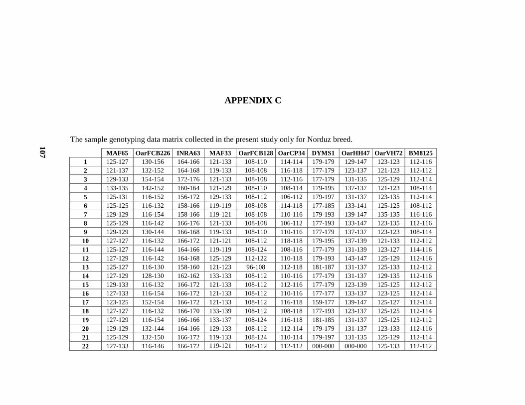
107
APPENDIX C
The sample genotyping data matrix collected in the present study only for Norduz breed.
MAF65 OarFCB226 INRA63 MAF33 OarFCB128 OarCP34 DYMS1 OarHH47 OarVH72 BM8125
1 125-127 130-156 164-166 121-133 108-110 114-114 179-179 129-147 123-123 112-116
2 121-137 132-152 164-168 119-133 108-108 116-118 177-179 123-137 121-123 112-112
3 129-133 154-154 172-176 121-133 108-108 112-116 177-179 131-135 125-129 112-114
4 133-135 142-152 160-164 121-129 108-110 108-114 179-195 137-137 121-123 108-114
5 125-131 116-152 156-172 129-133 108-112 106-112 179-197 131-137 123-135 112-114
6 125-125 116-132 158-166 119-119 108-108 114-118 177-185 133-141 125-125 108-112
7 129-129 116-154 158-166 119-121 108-108 110-116 179-193 139-147 135-135 116-116
8 125-129 116-142 166-176 121-133 108-108 106-112 177-193 133-147 123-135 112-116
9 129-129 130-144 166-168 119-133 108-110 110-116 177-179 137-137 123-123 108-114
10 127-127 116-132 166-172 121-121 108-112 118-118 179-195 137-139 121-133 112-112
11 125-127 116-144 164-166 119-119 108-124 108-116 177-179 131-139 123-127 114-116
12 127-129 116-142 164-168 125-129 112-122 110-118 179-193 143-147 125-129 112-116
13 125-127 116-130 158-160 121-123 96-108 112-118 181-187 131-137 125-133 112-112
14 127-129 128-130 162-162 133-133 108-112 110-116 177-179 131-137 129-135 112-116
15 129-133 116-132 166-172 121-133 108-112 112-116 177-179 123-139 125-125 112-112
16 127-133 116-154 166-172 121-133 108-112 110-116 177-177 133-137 123-125 112-114
17 123-125 152-154 166-172 121-133 108-112 116-118 159-177 139-147 125-127 112-114
18 127-127 116-132 166-170 133-139 108-112 108-118 177-193 123-137 125-125 112-114
19 127-129 116-154 166-166 133-137 108-124 116-118 181-185 131-137 125-125 112-112
20 129-129 132-144 164-166 129-133 108-112 112-114 179-179 131-137 123-133 112-116
21 125-129 132-150 166-172 119-133 108-124 110-114 179-197 131-135 125-129 112-114
22 127-133 116-146 166-172 119-121 108-112 112-112 000-000 000-000 125-133 112-112
107

108
23 125-127 116-132 164-166 129-133 108-112 108-110 000-000 137-145 121-123 112-112
24 125-127 116-146 156-160 133-133 108-112 118-118 179-179 133-141 127-137 108-108
25 127-127 116-156 166-172 133-133 108-124 110-116 189-189 137-147 123-135 110-116
26 125-127 116-130 166-166 121-133 108-108 110-110 179-189 131-149 123-135 108-114
27 125-129 116-138 156-166 133-139 108-110 108-116 000-000 123-145 125-135 112-112
28 129-129 116-152 164-166 121-129 108-112 110-112 175-177 135-137 127-135 112-112
29 119-127 116-138 166-170 121-133 96-108 112-116 159-179 123-131 123-127 112-118
30 127-127 116-130 166-172 121-129 108-108 108-112 000-000 000-000 121-123 112-112
31 129-129 116-128 166-170 133-133 108-122 108-116 179-183 141-149 125-125 112-112
32 119-127 130-132 166-172 119-133 108-122 110-116 175-181 133-137 123-133 112-112
33 125-127 116-116 164-166 131-131 108-112 108-116 179-179 123-135 123-123 112-114
34 127-129 132-132 168-176 133-133 108-110 112-116 179-179 137-145 125-129 112-114
35 125-131 128-148 166-172 121-121 108-112 112-118 179-187 123-137 123-137 112-112
36 127-135 152-156 164-172 133-133 108-120 110-114 177-193 145-147 123-133 112-116
37 127-129 130-146 164-166 121-129 108-110 116-116 179-179 131-139 125-131 112-116
38 127-129 116-152 166-172 121-129 108-110 112-118 175-183 135-137 123-133 108-112
39 121-127 116-152 164-168 119-133 108-112 110-116 179-189 129-131 129-135 116-116
40 127-129 116-116 164-166 129-133 108-110 112-116 179-185 137-137 127-133 112-118
41 129-129 116-138 164-172 121-121 108-112 112-116 159-193 123-145 123-133 112-112
42 125-127 116-152 158-164 119-121 108-110 108-110 183-189 137-147 125-135 114-116
43 127-129 138-152 166-172 133-144 108-108 116-118 189-193 133-147 129-133 112-116
44 127-127 142-154 166-172 129-133 108-112 108-108 177-177 139-139 123-123 112-116
45 127-129 116-150 160-170 131-133 108-124 114-116 177-193 135-137 125-135 112-112
46 125-129 132-132 166-176 121-133 108-120 110-118 173-189 131-143 123-125 108-112
108

109
MAF209 MCM140 MAF214 OarJMP29 OarFCB48 ILSTS5 OarJMP58 OarFCB20 OarFCB304 ILST11
1 114-114 180-186 188-188 134-142 147-149 192-199 159-165 93-106 163-163 271-284
2 114-124 180-186 190-190 122-132 147-158 186-199 140-159 93-102 179-189 271-276
3 112-116 180-182 188-188 134-136 000-000 192-194 140-140 93-93 179-183 276-284
4 114-114 182-186 190-190 132-134 147-154 192-199 140-151 93-93 163-165 276-284
5 114-124 178-186 188-190 134-134 147-162 192-199 140-165 89-93 163-169 270-284
6 112-112 184-188 188-190 124-132 147-149 192-199 151-159 89-102 183-189 271-284
7 116-124 184-184 188-188 134-136 147-149 192-192 147-155 93-93 163-173 271-271
8 114-116 178-180 188-188 134-134 147-162 192-199 140-140 93-102 171-179 281-284
9 112-116 180-184 190-190 124-155 144-147 192-199 149-149 89-93 161-179 278-284
10 114-124 178-186 188-188 132-134 144-147 192-199 140-140 86-93 163-167 271-278
11 124-126 000-000 188-190 134-134 147-147 188-196 140-151 91-91 163-189 276-284
12 114-124 184-184 190-190 142-142 144-147 192-199 140-157 89-89 163-165 271-284
13 114-124 182-184 190-190 136-136 169-171 192-192 147-151 91-102 165-179 271-284
14 114-116 184-184 188-190 132-136 162-162 192-199 140-159 100-108 161-165 276-284
15 112-124 182-190 190-190 134-146 154-171 192-192 140-157 93-102 173-177 271-284
16 112-114 182-182 188-190 132-142 154-167 196-199 140-147 91-102 177-177 276-284
17 114-114 172-180 188-190 122-122 147-162 192-199 140-140 86-93 163-177 276-276
18 114-114 180-186 190-190 136-151 147-162 190-199 159-165 89-93 179-183 276-284
19 124-124 174-178 190-190 126-132 147-147 192-192 165-165 91-91 169-173 276-284
20 112-124 178-186 190-190 134-134 147-147 192-196 140-147 91-100 163-165 276-276
21 114-114 180-186 188-190 000-000 144-147 192-199 147-159 100-104 163-163 284-284
22 110-122 186-188 188-188 126-134 144-147 192-192 140-165 100-100 165-179 276-281
23 114-128 184-186 188-188 136-136 147-149 199-199 140-147 89-106 163-163 271-284
24 116-130 172-184 190-190 122-132 147-147 192-199 140-140 91-102 161-163 284-284
25 122-122 184-186 190-190 134-155 142-147 194-194 140-140 93-100 163-183 271-271
26 114-124 184-184 188-190 136-142 147-164 192-199 147-147 89-100 179-179 271-284
27 114-128 180-188 190-190 000-000 000-000 000-000 000-000 89-114 183-185 271-278
28 114-124 184-186 190-190 132-132 144-156 186-199 140-155 89-114 147-179 271-278
29 110-114 176-184 188-188 000-000 000-000 190-213 140-161 86-106 163-185 271-284
109

110
30 114-114 182-190 188-190 122-134 142-169 192-199 151-159 91-104 161-163 276-276
31 114-122 172-172 190-190 124-132 144-144 192-199 140-140 91-97 177-183 276-276
32 114-128 180-184 188-188 132-134 147-162 192-192 147-165 100-106 163-167 271-284
33 112-114 176-184 188-188 126-134 162-162 192-199 140-140 100-100 163-179 276-284
34 114-114 180-182 188-188 132-136 147-149 186-199 155-165 91-93 179-187 271-276
35 112-114 180-188 188-188 132-132 147-164 192-199 140-151 95-100 165-171 276-284
36 116-124 184-190 190-190 134-134 142-147 192-192 140-155 91-100 165-165 271-276
37 112-122 184-184 190-190 124-134 144-147 192-192 140-161 100-100 165-187 270-284
38 114-114 184-186 190-190 132-142 147-169 192-194 151-165 102-106 163-179 276-284
39 114-124 182-184 188-188 124-155 154-171 196-199 149-165 91-102 161-163 276-284
40 114-116 178-180 188-188 132-146 147-162 192-192 140-140 89-104 165-171 271-276
41 114-124 180-182 190-190 132-134 147-154 186-192 165-165 102-104 165-171 284-284
42 114-124 184-184 188-188 132-134 144-147 192-199 140-159 89-93 161-163 271-284
43 124-124 184-186 190-190 132-132 142-149 192-196 140-155 89-102 177-189 284-284
44 114-114 180-184 190-190 134-134 147-154 192-192 151-165 91-93 161-163 276-284
45 114-114 184-184 190-190 134-146 147-147 192-199 140-151 91-93 161-163 271-276
46 114-124 182-184 190-190 130-132 147-162 186-196 140-149 91-114 161-171 276-276
110

111
APPENDIX D
The p-values of the linkage disequilibrium tests results. The first row is the breed names and the first column is the pairwise
comparison of 20 microsatellite loci. The abbreviations of the breeds are AKK for Akkaraman, CIC for Çine Çaparı, DAG for
Dağlıç, GOK for Gökçeada, HEM for HemĢin, HER for Herik, IVE for Ġvesi, KIV for Kıvırcık, KRG for Karagül, KRY for
Karayaka, MRK for Morkaraman, NOR for Norduz and SAK for Sakız. After Bonferroni corrections adjusted P-value for 5%
nominal level is: [0.05/171] = 0.00029.
SAK KRG HEM CIC NOR HER DAG MRK KIV KRG IVE GOK AKK
MAF65 X FCB226 0,96847 0,02126 0,89620 0,58819 0,84784 0,74541 0,18066 0,93030 0,61763 0,38911 0,63875 0,29406 0,91673
MAF65 X INRA63 0,91197 0,82389 0,10290 0,44966 0,03819 0,32047 0,05342 0,06700 0,26242 0,46507 0,02868 0,10160 0,59460
MAF65 X MAF33 0,70540 0,03999 0,59451 0,95049 0,93873 0,02292 0,64040 0,37418 0,31921 0,60630 0,79271 0,39890 0,00796
MAF65 X FCB128 0,78779 0,77611 0,11768 0,93358 0,63061 0,97420 0,07740 0,40058 0,73009 0,91448 0,37683 0,55508 0,88945
MAF65 X CP34 0,13554 0,35450 0,22364 0,32436 0,30873 0,89431 0,12395 0,42206 0,97503 0,61217 0,84694 0,15263 0,41334
MAF65 X DYMS1 0,07139 0,17575 0,50331 0,47672 0,35072 0,06732 0,87530 0,28844 0,71363 0,43228 1,00000 0,20430 0,58925
MAF65 X HH47 0,96026 0,98367 0,70713 0,62449 0,78927 0,40837 0,21039 0,96743 0,38171 0,29204 1,00000 0,85513 0,72188
MAF65 X VH72 0,05400 0,84053 0,94462 0,20477 0,88943 0,14600 0,57650 0,34267 0,63934 0,07609 0,02204 0,36464 0,72366
MAF65 X BM8125 0,51928 0,70895 0,38050 0,52580 0,94379 0,47998 0,44233 0,77276 1,00000 0,87092 0,63023 0,10169 0,11529
MAF65 X MAF209 0,11138 0,09348 0,08117 0,18952 0,30639 0,98713 0,48592 0,02629 0,27548 0,57656 0,93747 0,02206 0,58068
MAF65 X MCM140 0,88230 0,73779 0,20385 0,07881 0,24703 0,84708 0,14557 0,96770 0,54424 0,25306 1,00000 0,51482 0,13392
MAF65 X JMP29 0,22362 0,49336 0,90081 0,72958 0,91880 0,75250 0,52877 0,99498 0,12519 0,91986 0,32533 0,85893 0,53277
MAF65 X FCB48 0,65648 0,63549 0,89663 0,39748 0,82998 0,59564 0,68444 0,51860 0,75418 0,25553 0,42973 0,56925 0,87839
MAF65 X ILSTS5 0,73763 0,20371 0,78837 0,91107 0,66347 0,75504 0,41763 0,46815 0,33045 0,74249 0,84750 0,09892 0,04820
MAF65 X JMP58 0,03018 0,87530 0,94179 0,66734 0,98740 0,07229 0,93684 0,10567 1,00000 0,43673 0,71181 0,57805 0,74316
MAF65 X FCB20 0,93873 0,10706 0,16491 0,15648 0,79042 0,61343 0,24058 0,15349 1,00000 0,51928 0,70200 0,71086 0,59408
MAF65 X FCB304 0,26199 0,63194 0,74906 0,09067 0,45616 0,46725 0,20738 0,27481 0,87368 0,84757 0,94978 0,84804 0,31752
MAF65 X ILST11 0,72375 0,65290 0,15947 0,39561 0,08061 0,58448 0,31030 0,13866 0,04651 0,17440 0,46932 0,76307 0,69172
FCB226 X INRA63 0,10918 0,38646 1,00000 0,82638 0,90241 0,05945 0,85700 0,87348 0,11300 0,78277 0,54370 0,31858 0,95592
FCB226 X MAF33 0,09845 0,25112 1,00000 0,48320 0,96080 0,04993 0,59692 0,33079 0,95038 0,42580 0,71359 0,96221 0,70040
111

112
FCB226 X FCB128 0,00313 0,93471 0,05166 0,23399 0,04800 0,08747 0,07681 0,27949 0,50951 0,62506 0,42998 0,95816 0,32069
FCB226 X CP34 0,79928 0,79415 0,71352 1,00000 0,53644 0,20769 0,02456 0,86131 0,77960 0,47407 0,50949 0,73655 0,45079
FCB226 X DYMS1 0,23306 0,89611 0,69354 0,00924 1,00000 0,00477 0,97987 0,31892 0,97476 1,00000 0,34867 0,30360 0,74883
FCB226 X HH47 0,52281 1,00000 1,00000 0,47429 0,21554 0,93378 0,76844 0,53036 0,06993 0,71601 1,00000 0,84926 0,06278
FCB226 X VH72 0,39784 0,44004 1,00000 0,24060 0,20700 0,66959 0,83495 0,34505 0,05753 0,79127 0,73061 0,20648 0,15603
FCB226 X BM8125 0,60756 0,55295 0,47431 0,02830 0,47719 0,05079 0,91424 0,71730 0,56806 0,93176 0,54300 0,56093 0,27726
FCB226 X MAF209 0,50938 0,83581 1,00000 0,29726 0,17926 0,54184 0,30265 0,58169 0,94177 0,15931 0,95877 0,01451 0,05407
FCB226 X MCM140 0,39132 0,19143 0,19897 0,12467 0,83731 0,61712 0,56986 0,08142 0,48342 0,43081 0,30202 0,29269 0,84678
FCB226 X JMP29 0,98722 1,00000 1,00000 0,31649 1,00000 0,72679 0,54438 0,78140 0,17978 0,29318 0,41361 0,18686 0,57710
FCB226 X FCB48 0,36916 0,42458 0,62227 0,07623 0,91057 0,50461 0,93808 0,32971 0,11626 0,69402 0,88722 0,21988 0,01392
FCB226 X ILSTS5 0,59768 0,76955 0,90560 0,01343 0,78167 0,12663 0,25299 0,97591 0,37425 0,84190 0,31404 0,93446 0,92027
FCB226 X JMP58 0,84388 0,82899 0,32596 0,24420 0,86298 0,21721 0,06671 0,80362 0,80744 0,92987 0,23115 0,82690 0,12704
FCB226 X FCB20 0,15373 0,67193 1,00000 0,01790 0,62137 0,65929 0,92069 0,33340 1,00000 0,73592 0,74712 0,98225 0,22454
FCB226 X FCB304 0,60360 0,96035 0,24186 0,96905 0,60558 0,98268 0,81651 0,50753 0,02836 0,55956 0,76743 0,52519 0,96311
FCB226 X ILST11 0,96280 0,74771 1,00000 0,13293 0,27056 0,32281 0,88709 0,30157 0,89258 0,56059 0,62623 0,47908 0,50601
INRA63 X MAF33 0,37326 0,31480 0,28252 0,27447 0,11579 0,84663 0,99130 0,75022 0,17067 0,25974 0,10601 0,41921 0,40326
INRA63 X FCB128 0,51109 0,29431 0,35587 0,48500 0,10043 0,17611 0,00587 0,44746 0,01417 0,35949 0,93102 0,78887 0,55717
INRA63 X CP34 0,45286 0,65468 0,02910 0,26833 0,55634 0,39166 0,64982 0,79303 0,21217 0,88135 0,48529 1,00000 0,40616
INRA63 X DYMS1 0,96739 0,52861 0,98700 0,48833 0,30715 0,87589 0,99539 1,00000 0,51790 1,00000 1,00000 1,00000 1,00000
INRA63 X HH47 0,94242 0,70499 0,68201 0,22173 0,84719 0,26370 0,01667 0,06143 1,00000 1,00000 0,44510 1,00000 1,00000
INRA63 X VH72 0,11565 0,67978 0,47989 0,95996 0,82751 0,94924 1,00000 1,00000 0,74082 0,89674 0,39784 0,17213 0,14537
INRA63 X BM8125 0,44573 0,00511 0,17389 0,68167 0,43936 0,07206 0,67346 0,57803 0,14899 0,08695 0,54811 0,68972 0,39795
INRA63 X MAF209 0,52222 0,00371 0,44314 0,24507 0,56608 0,61309 0,50315 0,82726 0,07247 0,76352 0,67440 0,82173 0,61145
INRA63 X MCM140 0,73005 0,20915 0,54462 0,47101 0,50409 1,00000 0,03513 0,82332 1,00000 0,44354 1,00000 0,02530 0,26754
INRA63 X JMP29 0,40963 0,59780 0,54451 0,09944 0,49991 0,06779 0,54903 0,64786 0,55515 0,55780 0,82004 0,74314 0,36343
INRA63 X FCB48 0,34714 0,16134 0,10499 0,64163 0,38088 0,14136 0,04935 0,87901 1,00000 1,00000 0,24798 0,67393 0,90079
INRA63 X ILSTS5 0,90855 0,65841 0,78381 0,21867 0,94127 0,19757 0,33671 0,96984 0,56754 0,31682 0,37506 0,79557 0,16471
INRA63 X JMP58 0,73947 0,06631 0,99476 0,08178 0,54548 0,34247 0,76080 0,68171 0,12101 0,17955 0,58315 0,57674 0,13893
INRA63 X FCB20 0,50412 0,13185 0,63160 0,02341 0,86907 0,79127 0,90256 0,17135 1,00000 1,00000 0,26743 0,06984 0,40544
INRA63 X FCB304 0,36199 0,13108 0,54118 0,65661 0,54055 0,35513 0,45315 0,86071 0,88183 0,50313 0,67056 0,70715 0,18277
INRA63 X ILST11 0,84368 0,90333 0,01392 0,15522 0,93315 0,16147 0,60673 0,85362 0,55945 0,70576 0,49420 0,66453 0,25996
MAF33 X FCB128 0,04368 0,29710 0,07958 0,01788 0,52143 0,71507 0,03151 0,45319 0,00002 0,00090 0,58862 0,00148 0,73270
MAF33 X CP34 0,16370 0,03788 0,47449 0,02220 0,23558 1,00000 0,47848 0,24692 0,89422 0,96691 0,83821 0,55675 0,20387
MAF33 X DYMS1 0,62146 0,22011 0,71147 0,71113 0,66896 0,62206 0,09784 0,55931 0,87584 0,23608 0,56727 0,52335 0,19283
112

113
MAF33 X HH47 0,87816 0,04179 0,63444 0,01374 0,71057 0,68345 1,00000 0,97022 0,98896 0,58977 0,85664 1,00000 0,35448
MAF33 X VH72 0,75747 0,54422 0,17816 0,64831 0,83378 0,79782 0,87281 0,50628 0,81694 0,68653 0,12857 0,25846 0,84780
MAF33 X BM8125 0,50852 0,32233 0,69478 0,44946 0,91853 0,00358 0,15637 0,48763 0,94741 0,83761 0,47609 0,46361 0,41883
MAF33 X MAF209 0,78961 0,07474 0,16336 0,05774 0,86253 0,06532 0,98102 0,63754 0,69202 0,63707 0,86228 0,77040 0,11482
MAF33 X MCM140 0,13383 0,84633 0,67020 0,75783 0,39438 0,79879 0,89130 0,60137 0,73124 0,58441 0,92384 0,90929 0,44602
MAF33 X JMP29 0,57899 0,93788 0,70812 0,87742 0,08261 0,24238 0,87413 0,34350 0,29496 0,75832 0,65832 0,97168 0,24552
MAF33 X FCB48 0,99543 0,16462 0,81914 0,26095 0,33882 0,08662 0,23270 0,82564 0,99989 0,38142 0,08552 0,94699 0,13869
MAF33 X ILSTS5 0,48561 0,10484 0,60524 0,76795 0,92863 0,90148 0,23594 0,51534 0,84285 0,25551 0,65416 0,91170 0,11271
MAF33 X JMP58 0,29262 0,14438 0,74649 0,73716 0,24411 0,39953 0,36363 0,14413 0,74811 0,97164 0,55279 0,59213 0,63023
MAF33 X FCB20 0,94019 0,75265 0,72483 0,56723 0,93815 0,80511 0,06883 0,71793 0,35969 0,98014 0,97780 0,96044 0,59638
MAF33 X FCB304 0,90367 0,35735 0,08765 0,52425 0,93394 0,41930 1,00000 0,97960 0,92614 0,99809 0,29170 0,35045 0,37038
MAF33 X ILST11 0,83457 0,99143 0,70965 0,81107 0,89163 0,03016 0,57011 0,92274 0,46439 0,81066 0,36696 0,79982 0,34076
FCB128 X CP34 0,44705 0,53489 0,46750 0,22686 0,96332 0,06588 0,31055 0,24575 0,66192 0,95346 0,13270 0,58032 0,90978
FCB128 X DYMS1 0,21727 0,51610 0,55301 0,11811 0,39386 0,05720 0,46635 1,00000 0,04960 0,71386 0,45099 0,77805 0,76732
FCB128 X HH47 0,86471 0,56215 0,18707 0,74417 0,22020 0,35868 0,09658 0,55360 0,75920 0,33738 0,17589 0,49028 0,50873
FCB128 X VH72 0,69629 0,40013 0,67335 0,65891 0,76291 0,03954 1,00000 0,76044 0,84123 0,22584 0,19575 0,03682 0,06118
FCB128 X BM8125 0,74829 0,37481 0,17479 0,25614 0,48585 0,12112 0,54408 0,25052 0,66545 0,47409 0,50999 0,56271 0,06457
FCB128 X MAF209 0,65713 0,77020 0,15846 0,31835 0,30976 0,18183 0,57060 0,45785 0,46073 0,81741 0,85974 1,00000 0,61867
FCB128 X MCM140 0,96743 0,44537 0,03914 0,72767 0,98318 0,55218 0,50229 0,96383 0,60022 0,36921 0,96071 0,60771 0,19507
FCB128 X JMP29 0,47173 0,23291 0,25441 0,61082 0,39379 0,13718 0,89604 0,53372 0,38378 0,53950 0,96930 0,23041 0,31012
FCB128 X FCB48 0,86230 0,43763 0,48261 0,00144 0,13833 0,09600 0,75430 0,00202 0,95951 0,90866 0,15036 0,92461 0,03385
FCB128 X ILSTS5 0,39849 0,68864 0,73810 0,36892 0,91505 0,22767 0,39258 0,50819 0,67913 0,16073 0,42922 0,65592 0,14798
FCB128 X JMP58 0,98945 0,10648 0,37263 0,28898 0,36559 0,87420 0,04229 0,57746 0,91212 0,27598 0,90735 1,00000 0,35947
FCB128 X FCB20 0,03880 0,10396 0,00362 0,10673 0,00747 0,59809 0,59415 1,00000 0,69843 0,67105 1,00000 0,76383 1,00000
FCB128 X FCB304 0,64957 0,61903 0,00333 0,46050 0,85043 0,18365 0,45709 0,09606 0,66381 0,52809 0,83405 0,07989 0,28756
FCB128 X ILST11 0,06194 0,32704 0,65560 0,09359 0,65344 0,37224 0,80004 0,45601 0,66365 0,57287 0,31527 0,03909 0,87400
CP34 X DYMS1 0,19496 0,09687 0,25603 0,30472 0,64564 0,33585 0,98561 0,61698 0,64458 0,55668 0,41777 0,10416 0,54811
CP34 X HH47 0,31833 0,03934 0,01365 0,32229 0,80448 0,08725 0,56982 0,30011 0,61597 0,65819 0,41111 0,34150 0,76122
CP34 X VH72 0,34861 0,16862 0,68068 0,01075 0,50184 0,91446 1,00000 0,21489 0,74780 0,54251 0,91856 0,78970 0,21493
CP34 X BM8125 0,14843 0,29094 0,10877 0,14287 0,76170 0,77879 0,99897 0,99357 0,57560 0,54897 0,77002 0,47054 0,24591
CP34 X MAF209 0,53884 0,16975 0,87987 0,13257 0,99287 0,55933 0,08749 0,25360 0,43686 0,82991 0,83736 0,00470 0,25879
CP34 X MCM140 0,41939 0,81086 0,16161 0,75913 0,14847 1,00000 1,00000 0,10067 0,48668 0,59615 0,82094 0,44177 0,95839
CP34 X JMP29 0,49521 0,04094 0,13063 0,34786 0,59746 0,32526 0,97674 0,26430 0,69649 0,77114 0,36853 0,06129 0,88920
CP34 X FCB48 0,08216 0,82418 0,08812 0,58032 0,98734 0,28419 0,75142 0,12209 0,70180 0,27389 0,18837 0,12463 0,08099
113

114
CP34 X ILSTS5 0,50668 0,42571 0,85502 0,08574 0,91442 0,29456 0,30938 0,48342 0,00146 0,42323 0,54460 0,79987 0,01057
CP34 X JMP58 0,32944 0,64476 0,16637 0,27955 0,56646 0,87767 0,21221 0,29719 0,59991 0,31120 0,71824 1,00000 0,47971
CP34 X FCB20 0,45783 0,33736 0,94933 1,00000 0,81871 0,72695 0,73952 0,00583 0,70389 0,04388 0,76788 0,41156 0,40376
CP34 X FCB304 0,33300 0,08052 0,66790 0,37458 0,80254 0,91991 0,50133 0,21167 0,20666 0,28761 0,99363 0,20146 0,47085
CP34 X ILST11 0,27395 0,32083 0,72908 0,10861 0,24172 0,17206 0,96410 0,60133 0,93147 0,42049 0,63144 0,05574 0,03959
DYMS1 X HH47 0,50945 0,27179 0,86799 0,88493 1,00000 0,00544 0,89667 0,79485 0,82607 1,00000 0,40506 0,59233 1,00000
DYMS1 X VH72 0,07805 0,40569 0,87254 0,15902 0,89595 0,00162 0,91471 1,00000 0,82362 0,87301 0,89044 0,70682 0,94537
DYMS1 X BM8125 0,49017 0,01925 0,52184 0,72013 0,47998 0,28450 0,70254 0,10126 0,77355 0,72508 0,83259 0,10751 0,87593
DYMS1 X MAF209 0,23934 0,24370 0,58736 0,01788 0,55423 0,92857 0,68736 0,74238 0,07978 1,00000 0,78133 0,82515 0,00722
DYMS1 X MCM140 0,98893 0,55742 0,32987 0,77317 0,89969 0,81901 0,94426 1,00000 0,30940 1,00000 1,00000 1,00000 0,23875
DYMS1 X JMP29 0,25196 0,21568 0,62465 0,44444 0,43093 0,54800 0,12924 0,50340 0,55076 0,52924 0,57825 0,74681 0,92816
DYMS1 X FCB48 0,80268 0,31892 0,78250 0,59289 0,50083 0,27674 0,60121 1,00000 1,00000 0,32964 0,78504 0,90101 0,06613
DYMS1 X ILSTS5 0,97364 0,03306 0,51077 0,76104 0,74033 0,87791 0,89978 0,74586 0,40412 0,10515 0,99906 0,27879 0,71071
DYMS1 X JMP58 0,69687 0,85733 0,73509 0,76518 0,68158 0,75119 0,37892 0,26498 0,81377 0,41327 0,74541 0,18662 0,59042
DYMS1 X FCB20 0,34336 0,24253 0,17926 0,83819 0,30565 0,52895 0,59415 0,25223 0,61475 0,21849 0,49705 0,23390 1,00000
DYMS1 X FCB304 0,14890 0,39656 0,63311 0,15297 1,00000 0,38477 0,93664 0,67188 0,84125 0,81104 0,02011 0,53450 0,64413
DYMS1 X ILST11 0,23061 0,78273 0,06797 0,02989 0,65821 0,41080 0,24415 0,83752 0,56777 0,65461 0,49150 0,93630 0,35628
HH47 X VH72 0,44723 0,26165 0,51781 0,57848 0,76943 0,49683 1,00000 0,52973 0,51269 0,12395 0,71075 0,74780 0,80454
HH47 X BM8125 0,64966 0,33536 0,86264 0,87582 0,03401 0,83666 0,85583 0,75099 0,46433 0,71763 0,94514 0,77202 0,36464
HH47 X MAF209 0,41244 0,98075 0,77575 0,31626 0,83536 1,00000 0,45344 0,44051 0,67242 0,71242 0,57589 0,51867 0,01646
HH47 X MCM140 0,67515 0,78646 0,74681 0,44690 0,14399 0,59395 0,06644 0,58117 0,89294 0,06885 1,00000 0,35083 1,00000
HH47 X JMP29 0,04494 0,08394 0,93216 0,75241 0,65157 0,47485 1,00000 0,46536 0,85394 0,01251 0,29411 1,00000 1,00000
HH47 X FCB48 0,97386 0,00337 0,23718 0,49555 0,55418 1,00000 1,00000 0,39069 0,51849 0,32404 0,47928 1,00000 0,11260
HH47 X ILSTS5 0,22524 0,01525 0,60906 0,01451 0,86208 0,17458 0,03396 0,31775 0,02438 0,67380 0,87530 0,78322 0,98135
HH47 X JMP58 0,18851 0,44485 0,20115 0,14078 1,00000 0,41248 1,00000 1,00000 1,00000 0,75250 0,53729 1,00000 0,34501
HH47 X FCB20 0,31026 0,02022 0,16579 0,30421 1,00000 0,00893 1,00000 0,63203 0,59633 0,50700 0,32319 0,18995 0,36640
HH47 X FCB304 0,00913 0,17674 0,37805 0,91386 1,00000 0,20088 0,06012 0,64168 0,13430 0,95614 0,61583 0,58842 0,17024
HH47 X ILST11 0,59636 0,54489 0,06871 0,94573 0,92328 0,36696 0,75834 0,13072 0,86163 0,53099 0,65717 0,30072 0,89901
VH72 X BM8125 0,70762 0,41811 0,67562 0,08081 0,02618 0,44638 0,11244 0,46862 0,91709 0,02627 0,54148 0,31835 0,00322
VH72 X MAF209 0,82933 0,71084 0,29708 0,27051 0,81300 0,63979 0,73950 0,15418 0,01291 0,53558 0,07020 0,85124 0,57868
VH72 X MCM140 0,90331 0,42841 0,20434 0,94762 0,46714 0,66505 0,74665 0,95832 0,53097 0,64404 0,07501 0,87614 0,72542
VH72 X JMP29 0,40567 0,41694 0,57654 0,38860 0,07492 0,22054 0,92211 0,31977 0,04852 0,96356 0,87971 0,94051 0,11802
VH72 X FCB48 1,00000 0,89193 0,84816 0,13070 0,88057 0,23084 1,00000 0,97928 0,00031 0,41077 0,20834 0,50915 0,33349
VH72 X ILSTS5 0,21631 0,26673 0,02242 0,26968 0,14103 0,46419 0,98297 0,18846 0,96392 0,78511 0,14773 0,64973 0,29663
114

115
VH72 X JMP58 1,00000 0,78781 0,66334 0,10814 0,96300 0,14381 1,00000 0,77420 0,77924 0,93860 0,52973 0,66986 0,84910
VH72 X FCB20 0,67287 0,20976 0,46993 0,31561 0,77922 1,00000 0,61759 0,76673 0,48477 0,98313 1,00000 0,86754 0,06012
VH72 X FCB304 0,11143 0,62701 0,57978 0,02013 0,39015 0,69872 0,33399 0,20236 0,38214 0,85506 0,20720 0,95425 0,97971
VH72 X ILST11 0,39613 0,79615 0,04008 0,93650 0,94109 0,78009 0,85580 0,60052 0,87310 0,25281 0,11950 0,78365 0,74753
BM8125 X MAF209 0,73102 0,12825 0,87623 0,28111 0,20821 0,56520 0,84586 0,26613 0,13475 0,42960 0,02874 0,67060 0,74456
BM8125 X MCM140 0,70594 0,85783 0,56896 0,56035 0,65209 0,52679 0,18277 0,85331 0,90400 0,26149 0,72677 0,26437 0,55353
BM8125 X JMP29 0,17305 0,50603 0,58115 0,19719 0,03322 0,33414 0,66667 0,36610 0,84501 0,92204 0,95002 0,88707 0,34507
BM8125 X FCB48 0,30621 0,28448 0,23788 0,24568 0,99300 0,79901 0,23484 0,75920 0,37283 0,62447 0,29611 0,27164 0,53142
BM8125 X ILSTS5 0,36219 0,60020 0,45616 0,60587 0,08590 0,98306 0,97874 0,13941 0,28115 0,83549 0,46496 0,47555 0,34476
BM8125 X JMP58 0,29564 0,02366 0,67287 0,27782 0,84786 0,09534 0,63893 0,57380 0,52359 0,76583 0,44703 0,96842 0,25211
BM8125 X FCB20 0,37094 0,31271 0,02924 0,01208 0,73268 0,31730 0,23304 0,15778 0,62281 0,88133 0,50324 0,45171 0,78554
BM8125 X FCB304 0,99627 0,00796 0,17726 0,77411 0,18261 0,13315 0,44546 0,27830 0,50290 0,31581 0,35081 0,82445 0,64456
BM8125 X ILST11 0,66979 0,56050 0,39829 0,15801 0,88486 0,04503 0,57229 0,49327 0,88430 0,97937 0,96046 0,47173 0,67222
MAF209 X MCM140 0,17395 0,10798 0,05058 0,19730 0,02108 0,69852 0,73309 0,11577 0,82955 0,20223 0,21763 0,25906 0,93898
MAF209 X JMP29 0,95700 0,98466 0,12865 1,00000 0,77380 0,98729 0,72901 0,57114 0,79175 0,30207 0,45695 0,69055 0,68178
MAF209 X FCB48 0,08336 0,09399 0,04906 0,53088 0,37665 0,43650 0,04501 0,94076 0,93077 0,55767 0,64935 0,37033 0,50760
MAF209 X ILSTS5 0,53167 0,21212 0,35380 0,65560 0,25812 0,54870 0,84933 0,03621 0,48932 0,61741 0,36381 0,11095 0,98212
MAF209 X JMP58 0,16808 0,33974 0,24876 0,71714 0,63232 0,82341 0,88158 0,43648 0,14901 0,49647 0,03138 0,55220 0,43999
MAF209 X FCB20 0,65243 0,75272 0,45443 1,00000 0,19656 0,86370 0,22074 0,52607 0,61772 0,93012 0,17400 1,00000 0,89314
MAF209 X FCB304 0,99388 0,50735 0,79372 1,00000 0,17159 0,02843 0,12085 0,41597 0,50175 0,98590 0,67033 0,55729 0,12470
MAF209 X ILST11 0,19478 0,25432 0,03077 0,81275 0,16550 0,33754 0,46266 0,01188 0,12764 0,12737 0,94262 0,06228 0,05556
MCM140 X JMP29 0,11287 0,70409 0,32382 0,80470 0,56444 0,94350 0,58192 0,01134 0,20983 0,58668 0,37470 0,08700 0,01113
MCM140 X FCB48 0,47321 0,76673 0,03351 0,88722 0,45632 0,00643 0,36161 0,16057 0,67704 0,40664 0,46853 0,34656 0,53504
MCM140 X ILSTS5 0,17215 0,32964 0,23718 0,84008 0,39620 0,50137 0,10463 0,45369 0,63893 0,54166 0,22683 0,63399 0,61509
MCM140 X JMP58 0,58821 0,99879 0,16307 0,68372 0,26356 0,88648 0,67422 0,26914 0,87872 0,82256 0,65333 1,00000 0,01847
MCM140 X FCB20 0,55171 0,91480 0,71865 0,94064 0,79719 0,10517 0,52812 1,00000 0,10675 1,00000 0,69568 0,73545 1,00000
MCM140 X FCB304 0,54229 0,96993 0,13783 0,79701 0,40657 0,57524 0,67717 0,67321 0,46118 0,06093 0,19350 0,77287 0,18219
MCM140 X ILST11 0,51023 0,98686 0,20668 0,67063 0,99028 0,09561 0,13102 0,41248 0,70308 0,43999 1,00000 0,42454 0,70771
JMP29 X FCB48 0,78032 0,43018 0,78790 0,27800 0,21086 0,22150 0,95124 0,12976 0,89274 0,86790 0,85362 0,73176 0,12641
JMP29 X ILSTS5 0,40058 0,35250 0,20558 0,17708 0,83378 0,20711 0,97301 0,63603 0,82517 0,91264 0,87256 0,34483 0,07436
JMP29 X JMP58 0,13837 0,46480 0,06831 0,11028 0,90569 0,18151 0,93522 0,34651 0,84453 0,90999 0,24782 1,00000 0,38999
JMP29 X FCB20 0,70598 0,49055 0,69784 0,65011 0,06712 0,92233 0,13709 0,61646 0,65596 1,00000 0,05655 0,32895 0,13349
JMP29 X FCB304 0,45448 0,31505 0,30475 0,16480 0,64665 0,89694 0,93659 0,49771 0,35475 0,69231 0,01055 0,96188 0,18974
JMP29 X ILST11 0,00803 0,18491 0,04703 0,22126 0,71842 0,24834 0,81262 0,03938 0,33113 0,63918 0,38457 0,98570 0,10632
115

116
FCB48 X ILSTS5 0,70259 0,01246 0,10902 0,00619 0,15695 0,18893 0,96298 0,05310 0,44397 0,87764 0,65807 0,81624 0,24732
FCB48 X JMP58 0,58554 0,21161 0,95277 0,08390 0,56550 0,61489 0,85603 0,11901 0,23363 0,57883 0,66255 0,42474 0,14031
FCB48 X FCB20 0,94723 0,75083 0,13135 0,24908 0,09303 0,94298 0,94103 0,26622 0,65216 0,99026 0,59435 0,35931 0,62708
FCB48 X FCB304 0,03682 0,00659 0,14420 0,70220 0,55445 0,64330 0,32789 0,22218 0,42715 0,80879 0,61158 0,47413 0,93378
FCB48 X ILST11 0,18214 0,87452 0,44357 0,17908 0,70223 0,16280 0,74094 0,70574 0,61986 0,26622 0,61601 0,33219 0,10196
ILSTS5 X JMP58 0,69894 0,01455 0,30198 0,01381 0,16136 0,39091 0,99226 0,53534 0,35859 0,63000 0,20488 0,90198 0,90942
ILSTS5 X FCB20 0,49343 0,30666 0,65823 0,13187 0,59809 0,20378 0,22946 0,63428 0,16991 0,23929 0,65558 0,48025 0,31745
ILSTS5 X FCB304 0,98954 0,27317 0,24300 0,83153 0,16419 0,16253 0,83034 0,71478 0,70702 0,38983 0,65765 0,82117 0,52852
ILSTS5 X ILST11 0,95139 0,84193 0,93729 0,75879 0,40461 0,16763 0,68070 0,83698 0,05007 0,82272 0,10560 0,13403 0,37818
JMP58 X FCB20 0,46997 0,89978 0,01943 0,67964 0,83018 0,61365 1,00000 0,12220 0,19341 0,79037 0,38322 0,02881 0,40317
JMP58 X FCB304 0,05578 0,17312 0,06183 0,13534 1,00000 0,22537 0,63405 0,00911 0,93545 0,46934 0,80715 0,85241 0,45951
JMP58 X ILST11 0,15061 0,50292 0,68000 0,03954 0,61907 0,86635 0,60324 0,93963 0,85243 0,62715 0,39370 0,67470 0,32159
FCB20 X FCB304 0,00641 0,33947 0,22033 0,83709 0,17213 0,10632 0,07323 0,84026 0,73318 0,28300 0,04548 0,78538 0,93783
FCB20 X ILST11 0,04051 0,57989 0,24381 0,09975 0,28875 0,12301 0,99431 0,95587 0,65938 0,80996 0,26968 0,86044 0,92296
FCB304 X ILST11 0,02332 0,25650 0,72573 0,44804 0,44460 0,00074 0,67946 0,36316 0,11417 0,59759 0,63882 0,03333 0,09631
116

117
APPENDIX E
The following Converter Java class accepts an input document composed of lines of
the form “Loci:Population:Allele:Value” and generates a document which can be
input to the POPTREE2 software. Excerpts from both the input and generated output
is given below.
import java.util.*;
import java.io.*;
public class Converter {
private String inputFile;
private String outputFile;
private Vector<double[][]> data;
private String header = "13 populations\n1 SAK\n2 KRG\n3 HEM\n4 CIC\n5
NOR\n6 HER\n7 DAG\n8 MRK\n9 KIV\n10 KRY\n11 IVE\n12 GOK\n13 AKK";
private int[] sizes = {13, 15, 19, 14, 16, 8, 18, 14, 9, 10, 14, 13, 18, 13, 11, 19, 16,
23, 10};
private String[] locusNames = {"MAF65", "FCB226", "INRA63", "MAF33",
"FCB128", "CP34", "DYMS1", "HH47", "VH72", "BM8125", "MAF209",
"MCM140", "JMP29", "FCB48", "ILSTS5", "JMP58", "FCB20", "FCB304",
"ILST11"};
private String[] footers = {"# 98 100 94 78 92 96 100 98 90 98 90 100
100",
"# 94 92 96 80 92 98 98 100 90 100 86 100 100",
"# 98 100 88 80 92 96 100 98 88 100 102 100 100",
"# 98 98 94 80 92 98 100 100 90 100 100 94 96",
"# 98 100 92 80 92 98 100 100 90 96 100 98 96",
"# 96 100 94 80 92 80 96 86 90 96 98 98 96",
"# 98 98 88 78 84 82 94 94 90 94 84 96 96",

118
"# 96 96 86 76 88 84 92 88 86 92 82 98 88",
"# 96 94 92 78 92 92 76 100 90 100 102 100 94",
"# 98 98 84 80 92 90 98 100 90 94 102 100 96",
"# 98 98 92 60 92 86 86 98 90 88 102 92 98",
"# 98 98 92 80 90 86 98 100 90 90 102 92 98",
"# 88 90 86 78 86 90 100 100 90 98 100 78 100",
"# 82 100 92 78 86 98 98 100 90 98 96 94 100",
"# 96 100 94 76 90 96 100 100 84 100 98 72 96",
"# 90 86 94 78 90 94 100 100 72 100 94 74 100",
"# 98 100 96 80 92 98 100 100 90 100 102 100 100",
"# 98 100 96 80 92 92 100 100 90 100 102 100 100",
"# 98 100 96 78 92 94 100 100 90 100 86 96 98"};
public Converter(String input, String output) {
inputFile = input;
outputFile = output;
data = new Vector();
for(int i=0;i<19;i++) {
double[][] read=new double[sizes[i]][13];
for(int j=0;j<sizes[i];j++)
for(int k=0;k<13;k++)
read[j][k]=0.0;
data.addElement(read);
}
}
public void convert() {
readFile();
writeToFile();
}
private void writeToFile() {

119
try {
FileOutputStream fos = new FileOutputStream(new File(outputFile));
fos.write(header.getBytes());
for(int i=0;i<19;i++) {
fos.write(new String("\n\n@locus "+(i+1)+"
"+locusNames[i]+"\n").getBytes());
for(int j=0;j<sizes[i];j++) {
fos.write(new String((j+1)+" * ").getBytes());
for(int k=0;k<13;k++) {
fos.write(new String(data.elementAt(i)[j][k]+" ").getBytes());
}
fos.write("\n".getBytes());
}
fos.write(footers[i].getBytes());
}
fos.close();
} catch(Exception ex) {
ex.printStackTrace();
}
}
private void readFile() {
try {
BufferedReader buf = new BufferedReader(new InputStreamReader(new
FileInputStream(new File(inputFile))));
String line = null;
while((line = buf.readLine()) != null) {
String[] parts = line.split(":");
int locus = Integer.parseInt(parts[0])-1;
int population = Integer.parseInt(parts[1])-1;
int allel = Integer.parseInt(parts[2])-1;
double frequency = Double.parseDouble(parts[3]);

120
data.elementAt(locus)[allel][population] = frequency;
}
buf.close();
} catch(Exception ex) {
ex.printStackTrace();
}
}
public static void main(String argv[]) {
Converter converter = new Converter(argv[0], argv[1]);
converter.convert();
}
}
An excerpt from the input:
………………
1:12:13:0.050000
1:13:3:0.010000
1:13:4:0.020000
1:13:5:0.197979
1:13:6:0.389740
1:13:7:0.261966
1:13:8:0.055242
1:13:10:0.030000
1:13:11:0.010000
2:1:1:0.510638
2:1:2:0.010638
2:1:3:0.191489
2:1:4:0.031915
2:1:5:0.010638
2:1:6:0.010638
2:1:7:0.031915
121
2:1:8:0.021277
2:1:10:0.063830
2:1:11:0.010638
2:1:12:0.031915
2:1:13:0.042553
2:1:14:0.021277
2:1:15:0.010638
2:2:1:0.301573
2:2:2:0.162054
…………………
An excerpt from the output:
13 populations
1 SAK
2 KRG
3 HEM
4 CIC
5 NOR
6 HER
7 DAG
8 MRK
9 KIV
10 KRY
11 IVE
12 GOK
13 AKK
@locus 1 MAF65
1 * 0.0 0.02 0.0 0.0 0.0 0.0 0.01 0.010204 0.033333 0.0 0.0 0.0 0.0
2 * 0.0 0.01 0.042553 0.0 0.021739 0.020833 0.0 0.060676 0.022222 0.010204
0.033333 0.045201 0.0
3 * 0.0 0.0 0.010638 0.0 0.021739 0.010417 0.02 0.030612 0.077776 0.020408

122
0.044444 0.02 0.01
4 * 0.0 0.01 0.0 0.076923 0.01087 0.020833 0.0 0.010204 0.088889 0.040816
0.033333 0.01 0.02
5 * 0.166877 0.51 0.18085 0.128205 0.184782 0.322912 0.219429 0.193699
0.244443 0.289441 0.055556 0.135287 0.197979
6 * 0.477289 0.43 0.340423 0.397435 0.358693 0.406245 0.428193 0.407392
0.299999 0.291075 0.18993 0.492188 0.38974
7 * 0.200284 0.02 0.319148 0.333332 0.293475 0.08333 0.148355 0.152836
0.144443 0.128814 0.354105 0.09 0.261966
8 * 0.030612 0.0 0.063827 0.0 0.021739 0.052083 0.05 0.010204 0.033333 0.098768
0.124495 0.076471 0.055242
9 * 0.020408 0.0 0.0 0.025641 0.054348 0.052083 0.037376 0.030612 0.0 0.05102
0.0 0.03 0.0
10 * 0.081633 0.0 0.042553 0.038462 0.021739 0.03125 0.08 0.071429 0.044444
0.030612 0.055556 0.01 0.03
11 * 0.0 0.0 0.0 0.0 0.01087 0.0 0.0 0.020408 0.011111 0.0 0.012586 0.0 0.01
12 * 0.0 0.0 0.0 0.0 0.0 0.0 0.0 0.0 0.0 0.0 0.044444 0.02 0.0
13 * 0.0 0.0 0.0 0.0 0.0 0.0 0.0 0.0 0.0 0.0 0.011111 0.05 0.0
# 98 100 94 78 92 96 100 98 90 98 90 100 100
……
Furthermore, another Java Class was implemented to convert a proprietary text
format, which is generated from MS Excel, to FSTAT Software input format. The
Java Class is given below.
import java.io.*;
public class Analyze {
/**

123
* @param args
*/
public static void main(String[] args) {
int i, j, ln_num=0, h_allel=0, pop_num=0;
int[][] x;
x = new int[6105][21];
File file = new File("D:\\yeni_irk.txt");
FileWriter fstream = null;
try {
fstream = new FileWriter("D:\\hande.dat");
} catch (IOException e1) {
e1.printStackTrace();
}
BufferedWriter out = new BufferedWriter(fstream);
FileReader fr = null;
BufferedReader bis = null;
String tmp = "";
String[] temp, lok;
int lok_num=20, y=0;
temp = new String[lok_num];
lok = new String[lok_num];
String delimiter = "\t";
try {
fr = new FileReader(file);
bis = new BufferedReader(fr);
for(i=0; i<6105; i++)
for(j=0;j<lok_num;j++)
x[i][j]=0;

124
for (i=0; tmp != null; i++) {
tmp = bis.readLine();
if(tmp != null){
temp = tmp.split(delimiter);
for (j=0;j<temp.length; j++){
if (i==0)
lok[j]=temp[j];
if(i > 0)
x[i][j]=Integer.parseInt(temp[j]);
if(x[i][j]>85000 && x[i][j]%1000>h_allel)
h_allel=x[i][j]%1000;
}
}
}
ln_num=i;
pop_num=1;
for(i=1;i<ln_num-1;i++){
if(x[i-1][0]>x[i][0]){
pop_num++;
}
}
out.write((pop_num) + " " + (lok_num-1) + " " + h_allel + " 3" + "\r\n");
for(i=1;i<=(lok_num-1);i++)
out.write(lok[i] + "\r\n");
pop_num=1;
for(i=1;i<ln_num-1;i++){
if(x[i-1][0]>x[i][0]){
pop_num++;
}
if(i!=1){

125
out.write("\r\n");
}
out.write(pop_num + " ");
for(j=1;j<=(lok_num-1);j++){
if (x[i][j]==0)
out.write(" 000" +"000");
else if(x[i][j]/100<1000){
if(x[i][j]/100>100){
if((x[i][j]/100)%10!=0)
out.write(" 0" + (x[i][j]/1000) + (x[i][j]%1000));
else
out.write(" 0" + (x[i][j]/1000) + "0" + (x[i][j]%1000));
}
else if(x[i][j]/100<100)
out.write(" 0" + (x[i][j]/100) + "0" + (x[i][j]%100));
else
out.write(" " + x[i][j]);
}
else if(x[i][j]<100000){
if(x[i][j]/100>100){
if((x[i][j]/100)%10!=0)
out.write(" 0" + (x[i][j]/1000) + (x[i][j]%1000));
else
out.write(" 0" + (x[i][j]/1000) + "0" + (x[i][j]%1000));
}
else if(x[i][j]/100<100)
out.write(" 0" + (x[i][j]/100) + "0" + (x[i][j]%100));
else
out.write(" " + x[i][j]);
}
else
out.write(" " + x[i][j]);

126
y++;
}
}
out.close();
bis.close();
fr.close();
System.out.println("Veri dosyasi olusturuldu.");
} catch (FileNotFoundException e) {
e.printStackTrace();
} catch (IOException e) {
e.printStackTrace();
}
}
}
An excerpt for the Analyze Java Class is as follows:
MAF65 OarFCB226 INRA63 MAF33 OarFCB128
OarCP34 DYMS1 OarHH47 OarVH72 BM8125
MAF209 MCM140 OarJMP29 OarFCB48 ILSTS5
OarJMP58 OarFCB20 OarFCB304 ILST11
1 127129 116116 166166 119133 108108
108114 175179 133141 121129 112114
114118 188188 132134 147147 186199
159165 9191 171177 276284
2 127129 116130 166166 119121 108112
114116 173173 141145 121131 112114
114126 180180 132132 147160 192199
159165 8991 163177 281284
3 127127 130130 166166 119121 108108
114116 173193 137141 121127 112114

127
114126 180188 132132 147162 192192
147159 9191 163171 276284
4 129129 130150 164166 121133 108112
114116 175179 145145 127133 112116
126126 182188 132132 160162 192192
159159 9191 171177 276284
5 127129 130154 164166 127133 108120
114116 175175 123145 127127 112114
114124 180184 132132 147162 199199
140159 8693 171177 276284
6 127131 116116 166190 121123 108124
114114 175181 137139 129133 112116
118126 180180 132132 149162 199199
159159 9193 165171 276284
7 125129 138154 164166 123125 108122
118118 173181 133141 121127 112112
114114 184184 132132 142149 192194
153159 9191 171177 276276
8 127127 116150 166176 125133 108122
112116 175193 141147 123123 112112
114126 180180 132132 147149 192199
149159 100100 163187 276284
………………
The Analyze Java Class generates the following output format to be given to FSTAT
software:
13 19 286 3
MAF65
FCB226
INRA63
MAF33
FCB128

128
CP34
DYMS1
HH47
VH72
BM8125
MAF209
MCM140
JMP29
FCB48
ILSTS5
JMP58
FCB20
FCB304
ILST11
1 127129 116116 166166 119133 108108 108114 175179 133141 121129 112114
114118 188188 132134 147147 186199 159165 091091 171177 276284
1 127129 116130 166166 119121 108112 114116 173173 141145 121131 112114
114126 180180 132132 147160 192199 159165 089091 163177 281284
1 127127 130130 166166 119121 108108 114116 173193 137141 121127 112114
114126 180188 132132 147162 192192 147159 091091 163171 276284
1 129129 130150 164166 121133 108112 114116 175179 145145 127133 112116
126126 182188 132132 160162 192192 159159 091091 171177 276284
1 127129 130154 164166 127133 108120 114116 175175 123145 127127 112114
114124 180184 132132 147162 199199 140159 086093 171177 276284
1 127131 116116 166190 121123 108124 114114 175181 137139 129133 112116
118126 180180 132132 149162 199199 159159 091093 165171 276284
1 125129 138154 164166 123125 108122 118118 173181 133141 121127 112112
114114 184184 132132 142149 192194 153159 091091 171177 276276
1 127127 116150 166176 125133 108122 112116 175193 141147 123123 112112
114126 180180 132132 147149 192199 149159 100100 163187 276284
1 127129 116150 166188 123133 108122 112116 175193 141141 123133 112112
118126 180180 130130 000000 192201 159159 091100 165171 284284

129
1 125129 116116 166190 119121 108108 114114 175193 141145 121125 112118
126126 180184 130134 142162 188194 153159 091100 165173 276284
1 127127 116116 164166 119119 108108 108116 183193 133149 125129 118118
114126 182182 124132 147162 188194 153153 102104 179183 278284
1 127129 116152 166188 119133 108122 114116 193195 137151 123123 110110
114126 182184 124132 149154 192194 147153 086091 165171 271280
1 125127 116130 164188 121133 108108 110116 175193 137139 123125 114118
114126 180182 130130 000000 194199 147153 091102 145163 281284
1 125135 138148 164166 121133 108120 112116 167181 125145 125129 112112
114124 180182 130132 149154 192199 147157 086091 171187 276284
……..