biogeography-based optimization: synergies with evolutionary

BIOGEOGRAPHY-BASED OPTIMIZATION: SYNERGIES

WITH EVOLUTIONARY STRATEGIES, IMMIGRATION

REFUSAL, AND KALMAN FILTERS

DAWEI DU

Bachelor of Science in Electrical Engineering

South - Central University for Nationalities

July, 2007

submitted in partial fulfillment of the requirements for the degree

MASTER OF SCIENCE IN ELECTRICAL ENGINEERING

at the

CLEVELAND STATE UNIVERSITY

August, 2009

This thesis has been approved for the

Department of ELECTRICAL AND COMPUTER ENGINEERING

and the College of Graduate Studies by

Thesis Committee Chairperson, Dr. Dan Simon

Department/Date

Dr. Fuqing Xiong

Department/Date

Dr. Yongjian Fu

Department/Date

To my beloved wife Yuanchao Lu, and my entire family

ACKNOWLEDGMENTS

I would like to thank the following people: Dr. Dan Simon for all his diligent

guidance as my supervisor, and his unselfish help in all aspects of my study; and

Richard Rarick and Mehmet Ergezer for their patience in giving me all the help I

needed. I would also thank my wife and my entire family. Thanks for your support

in my life.

BIOGEOGRAPHY-BASED OPTIMIZATION: SYNERGIES

WITH EVOLUTIONARY STRATEGIES, IMMIGRATION

REFUSAL, AND KALMAN FILTERS

DAWEI DU

ABSTRACT

Biogeography-based optimization (BBO) is a recently developed heuristic al-

gorithm which has shown impressive performance on many well known benchmarks.

The aim of this thesis is to modify BBO in different ways. First, in order to improve

BBO, this thesis incorporates distinctive techniques from other successful heuristic

algorithms into BBO. The techniques from evolutionary strategy (ES) are used for

BBO modification. Second, the traveling salesman problem (TSP) is a widely used

benchmark in heuristic algorithms, and it is considered as a standard benchmark in

heuristic computations. Therefore the main task in this part of the thesis is to modify

BBO to solve the TSP, then to make a comparison with genetic algorithms (GAs).

Third, most heuristic algorithms are designed for noiseless environments. Therefore,

BBO is modified to operate in a noisy environment with the aid of a Kalman filter.

This involves probability calculations, therefore BBO can choose the best option in

its immigration step.

v

TABLE OF CONTENTS

Page

ABSTRACT . . . . . . . . . . . . . . . . . . . . . . . . . . . . . . . . . . . . v

LIST OF TABLES . . . . . . . . . . . . . . . . . . . . . . . . . . . . . . . . . ix

LIST OF FIGURES . . . . . . . . . . . . . . . . . . . . . . . . . . . . . . . . x

NOMENCLATURE . . . . . . . . . . . . . . . . . . . . . . . . . . . . . . . . xii

ACRONYMS . . . . . . . . . . . . . . . . . . . . . . . . . . . . . . . . . . . . xiv

CHAPTER

I. INTRODUCTION . . . . . . . . . . . . . . . . . . . . . . . . . . . . . . . 1

1.1 Introduction to Biogeography-based Optimization . . . . . . . . 1

1.2 Organization of Thesis . . . . . . . . . . . . . . . . . . . . . . . . 4

II. MODIFIED BBO BASED ON EVOLUTIONARY STRATEGY AND IM-

MIGRATION REFUSAL . . . . . . . . . . . . . . . . . . . . . . . . 8

2.1 Motivation for BBO Modification . . . . . . . . . . . . . . . . . . 8

2.2 Evolutionary Strategy . . . . . . . . . . . . . . . . . . . . . . . . 9

2.3 Immigration Refusal . . . . . . . . . . . . . . . . . . . . . . . . . 10

2.4 Modified BBO Algorithms . . . . . . . . . . . . . . . . . . . . . 12

2.5 Simulations . . . . . . . . . . . . . . . . . . . . . . . . . . . . . . 13

2.5.1 Parameter Specification . . . . . . . . . . . . . . . . . . . 13

2.5.2 Performance Comparisons . . . . . . . . . . . . . . . . . . 14

2.6 Analysis of Results . . . . . . . . . . . . . . . . . . . . . . . . . . 15

2.6.1 F-tests . . . . . . . . . . . . . . . . . . . . . . . . . . . . 16

2.6.2 T-tests . . . . . . . . . . . . . . . . . . . . . . . . . . . . 18

III. BBO SOLUTION FOR THE TRAVELING SALESMAN PROBLEM . 22

vi

3.1 The Traveling Salesman Problem . . . . . . . . . . . . . . . . . . 22

3.2 Modification of BBO for the TSP . . . . . . . . . . . . . . . . . 25

3.2.1 Parallel Computation . . . . . . . . . . . . . . . . . . . . 25

3.2.2 Sequence-based Information Exchange . . . . . . . . . . . 27

3.2.3 BBO/TSP Algorithm . . . . . . . . . . . . . . . . . . . . 29

3.3 Simulations . . . . . . . . . . . . . . . . . . . . . . . . . . . . . . 31

3.3.1 Parameter Specifications . . . . . . . . . . . . . . . . . . 34

3.3.2 Simulation Results and Analysis . . . . . . . . . . . . . . 35

IV. MODIFICATION OF BBO BASED ON KALMAN FILTER FOR NOISY

ENVIRONMENTS . . . . . . . . . . . . . . . . . . . . . . . . . . . . 38

4.1 Detrimental Effect of Noise . . . . . . . . . . . . . . . . . . . . . 39

4.2 The Kalman Filter . . . . . . . . . . . . . . . . . . . . . . . . . . 40

4.3 Probability Calculations . . . . . . . . . . . . . . . . . . . . . . . 42

4.3.1 Global Probability of Island-Switching . . . . . . . . . . . 42

4.3.2 Local Probability of Islands Switching . . . . . . . . . . . 50

4.4 The Fitness Contribution of a Single SIV . . . . . . . . . . . . . 54

4.5 Three Immigration Options . . . . . . . . . . . . . . . . . . . . . 58

4.5.1 Option One: No Island Re-evaluation . . . . . . . . . . . 58

4.5.2 Option Two: Immigrating Island Re-evaluation . . . . . . 59

4.5.3 Option Three: Emigrating Island Re-evaluation . . . . . . 60

4.5.4 Optimal Option Selection . . . . . . . . . . . . . . . . . . 60

4.6 Simulations . . . . . . . . . . . . . . . . . . . . . . . . . . . . . . 62

4.6.1 Parameter Specifications . . . . . . . . . . . . . . . . . . 62

4.6.2 Simulation Results and Analysis . . . . . . . . . . . . . . 63

V. CONCLUSION AND FUTURE WORK . . . . . . . . . . . . . . . . . . 66

5.1 Conclusion . . . . . . . . . . . . . . . . . . . . . . . . . . . . . . 66

vii

5.2 Future Work . . . . . . . . . . . . . . . . . . . . . . . . . . . . . 68

BIBLIOGRAPHY . . . . . . . . . . . . . . . . . . . . . . . . . . . . . . . . . 70

APPENDIX . . . . . . . . . . . . . . . . . . . . . . . . . . . . . . . . . . . . . 74

A. FOURTEEN BENCHMARKS . . . . . . . . . . . . . . . . . . . . . . . . 75

viii

LIST OF TABLES

Table Page

I The performance of the heuristic algorithms. . . . . . . . . . . . . . . 4

II Best performance of different BBOs after 100 Monte Carlo simulations. 14

III F-test values and thresholds. . . . . . . . . . . . . . . . . . . . . . . . 18

IV T-test values and P values. . . . . . . . . . . . . . . . . . . . . . . . . 20

V The coordinates of 15 cities. . . . . . . . . . . . . . . . . . . . . . . . 34

VI Results of the TSP using BBO/TSP and GA. . . . . . . . . . . . . . 36

ix

LIST OF FIGURES

Figure Page

1 The relationship of fitness of habitats (number of species), emigration

rate µ and immigration rate λ . . . . . . . . . . . . . . . . . . . . . . 11

2 The six options for three cities TSP. . . . . . . . . . . . . . . . . . . . 24

3 Schematic representation of parallel computation. . . . . . . . . . . . 26

4 One-point crossover in GA. . . . . . . . . . . . . . . . . . . . . . . . . 29

5 Flow chart for solving the TSP using modified BBO. . . . . . . . . . 31

6 Two parents of an offspring. . . . . . . . . . . . . . . . . . . . . . . . 32

7 The first step in cycle crossover. . . . . . . . . . . . . . . . . . . . . . 32

8 The second step in cycle crossover. . . . . . . . . . . . . . . . . . . . 33

9 The third step in cycle crossover. . . . . . . . . . . . . . . . . . . . . 33

10 The final step in cycle crossover. . . . . . . . . . . . . . . . . . . . . . 34

11 The shortest path of 15 cities achieved by BBO/TSP. . . . . . . . . . 36

12 The shortest path of 15 cities achieved by GA. . . . . . . . . . . . . . 37

13 The PDF of the fitness of an island. . . . . . . . . . . . . . . . . . . . 43

14 The PDF of noise involved in the fitness. . . . . . . . . . . . . . . . . 43

15 The PDF of noises with different ranges, when b > c. . . . . . . . . . 46

16 The PDF of noises with different ranges, when c > b. . . . . . . . . . 46

17 The PDFs of the measured fitnesses of immigrating island and emi-

grating island in scenario 1. . . . . . . . . . . . . . . . . . . . . . . . 51





x



21 The PDFs of the fitness contributions of iSIV and rSIV in scenario 1. 55




25 The three options in the immigration step. . . . . . . . . . . . . . . . 61

26 The maximum fitnesses of RBBO, KBBO and NBBO after 100 Monte

Carlo simulations . . . . . . . . . . . . . . . . . . . . . . . . . . . . . 64

27 The mean fitnesses of RBBO, KBBO and NBBO after 100 Monte Carlo

simulations. . . . . . . . . . . . . . . . . . . . . . . . . . . . . . . . . 65

xi

NOMENCLATURE

α - number of parents in ES

β - number of children in ES

λ - immigration rate in BBO

µ - emigration rate in BBO

E - maximum possible value for emigration rate to the habitat

f - fitness of island

f1 - fitness of island 1

f2 - fitness of island 2

g - measured fitness in Kalman filter

G - number of groups of data in F-test

I - maximum possible value for immigration rate

K - number of population members need to be evaluated in ES

m - estimated fitness in Kalman filter

n - number of islands

n1 - fitness noise of island 1

n2 - fitness noise of island 1

N - number of experiments per group in F-test

N1 - number of dependent values in group 1 in T-test

N2 - number of dependent values in group 2 in T-test

P - fitness variance uncertainty in Kalman filter

Q - variance of process noise in Kalman filter

R - variance of observation noise in Kalman filter

xii

S - number of species in one habitat

S0 - equilibrium number of species in one habitat

Smax - maximum number of species one habitat can support

Sw - within-group variance in F-test

Sb - between-group variance in F-test

S1 - standard deviation of group 1 in T-test

S2 - standard deviation of group 2 in T-test

xiii

ACRONYMS

ACO ant colony optimization

BBO biogeography-based optimization

BBO/ES BBO with features borrowed from ES

BBO/RE BBO with immigration refusal

BBO/ES/RE BBO with features borrowed from ES and immigration refusal

DE differential evolution

ES evolutionary strategy

GA genetic algorithm

HSI habitat suitability index

KBBO BBO is modified based on Kalman filter

LS local search

NBBO BBO in noiseless environment

PBIL population-based incremental learning

PDF probability density function

PSO particle swarm optimization

QAP quadratic assignment problem

xiv

RBBO basic (regular) BBO, equivalent to BBO

SGA stud genetic algorithm

SIV suitability index variable

TSP Traveling salesman problem

xv

CHAPTER I

INTRODUCTION

Heuristic optimization is a new approach which can be used to solve complex

problems. It can overcome many shortcomings of more traditional methods [8]. The

research area of heuristic optimization algorithms has been attracting researchers for

the last 50 years, and numerous algorithms have been published [2]. Some of them,

such as genetic algorithms (GAs) and evolutionary strategy (ES), have been used to

solve many problems, which are very difficult to solve using traditional optimization

algorithms [2]. The importance of heuristic algorithms are generally recognized by

the engineering research community. More and more researchers choose heuristic

algorithms for different kinds of hard-to-solve problems.

1.1 Introduction to Biogeography-based Optimiza-

tion

As its name implies, Biogeography-based optimization (BBO) is based on the

science of biogeography. Biogeography is the study of the distribution of animals

1

2

and plants over time and space. Its aim is to elucidate the reason of the changing

distribution of all species in different environments over time. As early as the 19th

century, biogeography was first studied by Alfred Wallace [4] and Charles Darwin [5].

After that, more and more researchers began to pay attention to this area.

The environment of BBO corresponds to an archipelago, where every possible

solution to the optimization problem is an island. Each solution feature is called a

suitability index variable (SIV). The goodness of each solution is called its habitat

suitability index (HSI), where a high HSI of an island means good performance on

the optimization problem, and a low HSI means bad performance on the optimiza-

tion problem. Improving the population is the way to solve problems in heuristic

algorithms. The method to generate the next generation in BBO is by immigrat-

ing solution features to other islands, and receiving solution features by emigration

from other islands. The mutation is performed for the whole population in a manner

similar to the mutation in genetic algorithms (GAs).

The basic procedure of BBO is as follows:

1. Define the island modification probability, mutation probability, and elitism

parameter. Island modification probability is similar to crossover probability in

GAs. Mutation probability and elitism parameter are the same as in GAs.

2. Initialize the population (n islands).

3. Calculate the immigration rate and emigration rate for each island. Good so-

lutions have high emigration rates and low immigration rates. Bad solutions

have low emigration rates and high immigration rates. (The emigration rate

and immigration rate will be introduced in the next chapter.)

4. Probabilistically choose the immigrating islands based on the immigration rates.

Use roulette wheel selection based on the emigration rates to select the emigrat-

3

ing islands.

5. Migrate randomly selected SIVs based on the selected islands in the previous

step.

6. Probabilistically perform mutation based on the mutation probability for each

island.

7. Calculate the fitness of each individual island.

8. If the termination criterion is not met, go to step 3; otherwise, terminate.

In 2008, biogeography was applied to engineering optimization [3] for the first

time. Fourteen benchmarks were used to test the performance of various heuristic

algorithms. The algorithms that were tested include:

1. ACO - ant colony optimization

2. BBO - biogeography-based optimization

3. DE - differential evolution

4. ES - evolutionary strategy

5. GA - genetic algorithm

6. PBIL - population-based incremental learning

7. PSO - particle swarm optimization

8. SGA - stud genetic algorithm

The results shown in Table I are the best results after 100 Monte Carlo sim-

ulations of each algorithm, where the best performances are normalized to 100 in

each row. In Table I, BBO has good performances compared to the other algorithms.

4

Table I: The performance of the heuristic algorithms. The best performance of all algo-rithms on each benchmark is normalized to 100 [3].

Though BBO is outperformed on ten benchmarks, its performances are usually only

slightly worse than the winners. BBO performs the best on four benchmarks, the

second best on seven benchmarks, and the third best on the other three benchmarks.

This indicates that BBO is an algorithm that has much promise and merits further

development and investigation.

The details of all benchmarks used in Table I are shown in Appendix A. The

purpose of benchmarks is to test the performance of heuristic algorithms. There is

no physical meaning for most of the benchmarks.

1.2 Organization of Thesis

The goal of the second chapter of the thesis is to improve the performance of

BBO by adding two techniques, one of which is taken from ES, and the other is called

immigration refusal. Although it is shown that BBO has the ability to solve opti-

mization problems in [3], in order to maintain the advantage of BBO compared with

other heuristic algorithms, it is necessary to improve BBO by borrowing techniques

from other algorithms. As a successful heuristic algorithm, evolutionary strategy (ES)

has an important historic position in the field of heuristic algorithm [8]. It has been

5

used for over three decades, and is still widely used in many areas. Since ES has

demonstrated good performance solving complex and difficult problems, borrowing a

technique from ES is a good place to start in the investigation. The addition of ES

features to BBO is an original contribution of this thesis [1].

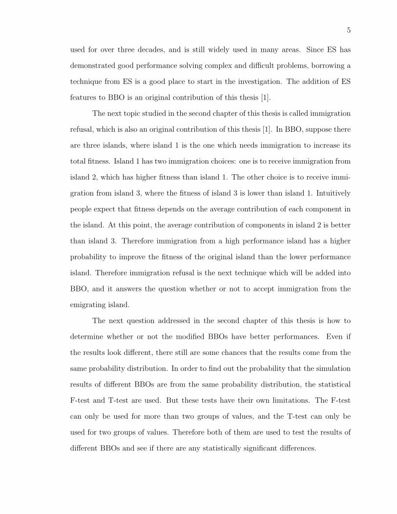
The next topic studied in the second chapter of this thesis is called immigration

refusal, which is also an original contribution of this thesis [1]. In BBO, suppose there

are three islands, where island 1 is the one which needs immigration to increase its

total fitness. Island 1 has two immigration choices: one is to receive immigration from

island 2, which has higher fitness than island 1. The other choice is to receive immi-

gration from island 3, where the fitness of island 3 is lower than island 1. Intuitively

people expect that fitness depends on the average contribution of each component in

the island. At this point, the average contribution of components in island 2 is better

than island 3. Therefore immigration from a high performance island has a higher

probability to improve the fitness of the original island than the lower performance

island. Therefore immigration refusal is the next technique which will be added into

BBO, and it answers the question whether or not to accept immigration from the

emigrating island.

The next question addressed in the second chapter of this thesis is how to

determine whether or not the modified BBOs have better performances. Even if

the results look different, there still are some chances that the results come from the

same probability distribution. In order to find out the probability that the simulation

results of different BBOs are from the same probability distribution, the statistical

F-test and T-test are used. But these tests have their own limitations. The F-test

can only be used for more than two groups of values, and the T-test can only be

used for two groups of values. Therefore both of them are used to test the results of

different BBOs and see if there are any statistically significant differences.

6

The third chapter in this thesis is about the traveling salesman problem (TSP),

which is a problem that can be easily understood but not easily solved by traditional

methods. Because of its characteristics, the TSP is one of the standard benchmarks

in heuristic algorithms. Even without its theoretical importance, the TSP also has

practical significance, for example, in the manufacture of microchips, or task planning.

In order to increase the calculation speed of BBO, parallel computation is added into

BBO to boost its calculation speed when it encounters long calculation times like those

that arise in the TSP. In the third chapter of this thesis, BBO which is combined with

parallel computation is used to solve the TSP. The application of BBO to the TSP

is another original contribution of this thesis. Also, a comparison of BBO and GA is

used to determine the performance of BBO in the TSP solution.

The fourth chapter in this thesis is the consideration of noisy optimization

problems. For the original BBO and most other heuristic algorithms, their environ-

ments are assumed to be noiseless. That means that the fitness of each gene or island

calculated in the algorithm is true and accurate. Based on these accurate fitnesses,

the algorithms continue their operations step by step. But in the real non-ideal world,

a pure noiseless environment never exists. Also, the final purpose for all algorithms is

to contribute to the real world — the noisy world. Therefore how to deal with noise

is another challenging question for all heuristic algorithms.

The main task in the fourth chapter of this thesis is the application of the

Kalman filter to BBO to counteract the effect of noise, and to provide a good fitness

estimate in every generation. This is the final original contribution of this thesis. Be-

cause of noise, calculated fitnesses are not the true fitnesses; they are the combinations

of true fitness and noise. Therefore how to choose the right island for immigration

and emigration is another problem that needs to be solved. Probability-based selec-

tion is introduced into BBO as another new technique. It calculates all the possible

7

probabilities ahead of time, then helps BBO to make the best decision based on the

calculated probabilities in the immigration step. This technique can provide BBO the

choice which has the highest probability to make an improvement in the immigration

step with only a little extra calculation. With this technique, BBO can decrease the

chance of making mistakes in the immigration step.

The last chapter includes conclusions and directions for future work.

CHAPTER II

MODIFIED BBO BASED ON

EVOLUTIONARY STRATEGY AND

IMMIGRATION REFUSAL

2.1 Motivation for BBO Modification

A hybrid evolutionary algorithm is an attempt to combine two or more evo-

lutionary algorithms. This can get the best from the algorithms that are combined

together. Each heuristic algorithm has its own advantages with respect to robust-

ness, performance in noisy environments, performance in the presence of uncertain

parameters, or performance on different types of problems. At the same time, no

algorithm can avoid marginal performance on certain problems. Hybrid algorithms

can combine the advantages of each algorithm and avoid their disadvantages.

For example, in [6], ACO, GA and local search (LS) are combined to solve

the quadratic assignment problem (QAP). ACO is used to construct a good initial

population and provide feedback to the GA. With a well-constructed initial population

8

9

instead of a random one, the GA is used to solve the QAP. After obtaining the

solution using GA and ACO, LS can be used to improve this solution. When these

three algorithms are combined, their advantages are combined too. Reference [6]

demonstrates that the hybrid evolutionary algorithm gives outstanding performance

compared with the algorithms acting separately.

There are also many other examples of hybrid heuristic algorithms. For ex-

ample, PSO and incremental evolution strategy (PIES) have been combined to solve

function optimization problems in Chapter 5 of [7]. The combination of GA and

bacterial foraging is another hybrid evolutionary algorithm for solving function op-

timization problems in Chapter 8 of [7]. Hybrid heuristic algorithms can perform

significantly better than a single heuristic algorithm. Because of this advantage,

more and more attention has focused on the hybrid evolutionary algorithm field in

recent years.

2.2 Evolutionary Strategy

Evolutionary strategy was created by students at the Technical University of

Berlin in the 1960s and 1970s. It is one of the classic optimization techniques among

heuristic methods. The basic procedure of the evolutionary strategy algorithm can

be described as follows [8]:

1. Define α as the number of parents and β as the number of children.

2. Initialize the population of α individuals.

3. Perform recombination using the α parents to form β children.

4. Perform mutation on all the children.

5. Evaluate K population members, where K ∈ [α, α + β].

10

6. Out of the K individuals in the previous step, select α individuals for the new

population.


In step 5, users can evaluate either α + β population members or just the β

children. If α = β, and all α + β individuals are evaluated, the probability of getting

fitter individuals for the next generation is increased dramatically. Likewise, if this

method is used in BBO, the chance of finding the best island can be increased. If

set α = β, and K = α + β, the fitness values of the α parents have already been

calculated in the previous generation, therefore the burden of cost function evaluation

does not increase relative to the standard BBO algorithm.

In many realistic problems, the cost function evaluation of the population is

computationally expensive. Therefore if the α + β option of ES is used, the probabil-

ity of finding the best island can be significantly increased without introducing more

calculation. That is the reason this feature from ES is added to BBO.

2.3 Immigration Refusal

In BBO, the emigration rate and immigration rate are used to determine to

where to emigrate and from where to get immigration. Figure 1 shows the relation-

ships between fitness of habitats (number of species), emigration rate µ and immigra-

tion rate λ. E is the possible maximum value of emigration rate to the habitat, and

I is the possible maximum value for immigration rate. S is the number of species in

this habitat, which corresponds to fitness. Smax is the maximum number of species

the habitat can support. S0 is the equilibrium value; when S = S0, the emigration

rate µ is equal to the immigration rate λ.

From Figure 1, it is clear that the island which has good performance like S2

11

Figure 1: The relationship of fitness of habitats (number of species), emigration rate µand immigration rate λ [3].

has a high emigration rate and a low immigration rate. On the other hand, the island

which has poor performance like S1 has a high immigration rate and a low emigration

rate.

In the original BBO, where to emigrate and from where to receive immigration

are based on the emigration rate and immigration rate. If the island has a high

emigration rate, the probability of emigrating to other islands is high. On the other

hand, the probability of immigration from other islands is low. But the low probability

does not mean that immigration will never happen. Once in a while a highly fit

solution will immigrate solution features from a low-fitness solution. This may ruin

the high fitness of the island which receives the immigrants. Therefore when the

solution features from an island which has low fitness try to emigrate to other islands,

the other islands should carefully consider whether or not to accept these immigrants.

That is, if the emigration rate of the island which sends the solution feature is less

than some thresholds, and its fitness is also less than that of the immigrating island,

the immigrating island will refuse the immigrating solution features. This idea, called

immigration refusal, is what is added to BBO.

12

2.4 Modified BBO Algorithms

First, borrow the technique from ES. That is, for every generation, evaluate α

+ β individuals, where α = β. Second, add the immigration refusal approach to BBO.

This will decrease the potential harm from low fitness islands. With the combination

of these two techniques, the following modifications are made to BBO.

1. Original BBO

2. BBO with techniques borrowed from ES (BBO/ES)

3. BBO with immigration refusal (BBO/RE)

4. BBO with techniques borrowed from ES and immigration refusal (BBO/ES/RE)

The basic procedure of BBO/ES is as follows:

1. – 5. are the same as 1. – 5. in original BBO described in Section 1.1.


child island.

7. Calculate the fitness of each individual island, including both parent and child

islands. Store them for the use in the next generation.

8. Based on the techniques borrowed from ES, select the best n islands from the

n parents and n children as the population for the next generation.


The basic procedure of BBO/RE is as follows:

1. – 4. are the same as 1. – 4. in original BBO described in Section 1.1.

13

5. Migrate randomly selected SIVs based on the selected islands in the previous

step. When receiving immigration from other islands, use the immigration

refusal idea to decide whether or not to accept the immigration.


child island.

7. Calculate the fitness of each individual island.


The basic procedure of BBO/ES/RE is as follows:

1. – 5. are the same as 1. – 5. in BBO/RE.

6. – 9. are the same as 6. – 9. in BBO/ES.

2.5 Simulations

2.5.1 Parameter Specification

The simulation parameters are as follows:

• Number of Monte Carlo simulations: 100

• Number of islands: 100

• Number of SIVs per island: 20

• Generations per Monte Carlo simulation: 100

• Mutation probability: 0.005

• Elitism parameter: 1

14

Note that the number of islands is the population size, the number of SIVs per island

is the problem dimension, and the elitism parameter is the number of elite islands

saved for the next generation. The threshold of immigration refusal is 0.5. When the

emigration rate is larger than 0.5, where emigration rate is normalized from 0 to 1,

immigration refusal does not apply. When the emigration rate is less than 0.5, the

island only accepts immigration if it comes from an island which has better fitness.

2.5.2 Performance Comparisons

Table II shows the performance of the four different BBOs. See [3] for a

description of the 14 benchmarks used in this study. The differences in performance

between the BBOs can be summarized as follows:

Table II: Best performance of different BBOs after 100 Monte Carlo simulations.BBO BBO/ES BBO/RE BBO/ES/RE

Ackley 3.56 1.34 3.03 1.42Fletcher 9570.10 4503.96 6216.63 2248.52Griewank 1.40 1.04 1.42 1.07Penalty # 1 1.05 0.04 1.10 0.03Penalty # 2 4.07 0.46 4.56 0.51Quartic 3.68E-04 4.81E-06 2.22E-04 6.33E-06Rastrigin 1.93 0.00 4.04 0.00Rosenbrock 17.83 12.80 21.41 13.44Schwefel 1.2 51.41 9.52 28.69 12.10Schwefel 2.21 680.93 654.65 866.16 889.69Schwefel 2.22 0.80 0.10 0.70 0.10Schwefel 2.26 10.70 8.40 10.50 9.30Sphere 0.16 0.00 0.12 0.01Step 62.00 7.00 39.00 7.00

1. BBO/ES vs. BBO: With the techniques borrowed from ES, BBO/ES has a bet-

ter performance than BBO. This is especially true for the Penalty #1, Penalty

#2, Quartic, Rastrigin and Sphere functions, where BBO/ES is more than ten

times better than BBO.

15

2. BBO/RE vs. BBO: BBO/RE outperforms BBO 8 out of 14 times, and BBO

performs better than BBO/RE 6 out of 14 times, therefore it is not clear whether

or not BBO/RE is better than BBO.

3. BBO/ES/RE vs. BBO: BBO/ES/RE performs better than BBO every time.

The improved performance is especially large for the Penalty #1, Quartic, Ras-

trigin and Sphere functions, where BBO/ES/RE is more than 10 times better

than BBO.

4. BBO/ES outperforms both BBO and BBO/RE every time. BBO/ES/RE out-

performs BBO and BBO/RE almost every time, losing only one time. In other

words, the techniques borrowed from ES have a strong effect on BBO, and

increase the performance of BBO a lot.

5. BBO/ES/RE outperforms BBO/ES two out of 14 times, has the same perfor-

mance three times, and has worse performance nine times.

From the values shown in Table II, the techniques borrowed from ES give BBO

a large improvement, but the effect of the immigration refusal does not have a large

impact. Therefore tuning the parameters of immigration refusal is an area for future

research.

2.6 Analysis of Results

From Table II, it shows the differences between different kinds of BBOs. But

without any statistical analysis, conclusions drawn from Table II are only a subjective

judgement. In this section, there are two statistical methods used to analyze the

differences between different BBOs: F-tests and T-tests. These two methods can give

us the confidence level that the differences between simulation results are statistically

significant.

16

2.6.1 F-tests

The F-test is a statistical test for several groups of numbers, where the number

of groups is greater than two. The F-test can be summarized as follows [9].

1. G is the number of groups of data, where each group is distinguished by some

set of independent variables. N is the number of experiments per group.

2. Calculate Xg as follows.

Xg =1

N

N∑i=1

Xgi (2.1)

Xg is the average value of the dependent variable for group g. Xgi is the

dependent variable of the i-th experiment for group g.

3. Calculate X as follows.

X =1

NG

G∑g=1

N∑i=1

Xgi (2.2)

X is the average value of the entire population including all groups.

4. Calculate the within-group variance as follows.

Sw =1

G

G∑g=1

1

N − 1

N∑i=1

(Xgi −Xg)2 (2.3)

5. Calculate the between-group variance as follows.

Sb =1

G− 1

G∑g=1

(X −Xg)2 (2.4)

6. The F-test value is equal to Sb/Sw

The F-test value can be used as follows in order to determine if the differences

between the groups of data are statistically significant [10].

17

1. The user chooses a probability P . This is the probability that the groups of

data are from the same distribution. As an example, if the user wants to have

a 99% confidence that there is a statistically significant difference between the

groups of data, then P=0.01.

2. Compute the F-test value from the procedure above.

3. The numerator degrees of freedom is defined as G − 1, and the denominator

degrees of freedom is defined as NG−G.

4. According to the P value, numerator degrees of freedom, and denominator

degrees of freedom, the F-test threshold from tables can be found such as those

given in [11].

5. If the F-test value is larger than the threshold, that means there is a probability

P or less that results of the groups are from the same distribution.

In this chapter, there are fourteen benchmarks used to test different BBOs. For

each benchmark, each of the four BBOs is run for 100 Monte Carlo simulations. That

means for each benchmark, each BBO converges to 100 different minimum values.

Table III shows the F-test values for each benchmark, along with the F-test

thresholds for the 95%, 99%, and 99.9% confidence levels. If the F-test value is greater

than the threshold for some P , that means the BBO differences are statistically

significant with a probability of 1− P or greater.

The F-test results can be summarized as follows:

1. When P = 0.05, on Ackley, Griewank, Penalty #1, Rastrigin, Schwefel 1.2,

Schwefel 2.22, Sphere, and Step, the F-test values are larger than the threshold.

Therefore with 95% (or greater) confidence, on these benchmarks, the differ-

ences between the different BBOs are statistically significant and are not from

the same distribution.

18

Table III: F-test values and thresholds.Benchmark F-test value Threshold

P = 0.001 P = 0.01 P = 0.05Ackley 6.23Fletcher 0.29Griewank 3.74Penalty # 1 3.65Penalty # 2 0.16Quartic 1.64Rastrigin 5.40 5.51 3.82 2.62Rosenbrock 0.20Schwefel 1.2 2.90Schwefel 2.21 0.05Schwefel 2.22 3.14Schwefel 2.26 0.29Sphere 4.04Step 3.68

2. When P = 0.01, on Ackley, Rastrigin, and Sphere, the F-test values are bigger

than the threshold. Therefore with 99% (or greater) confidence, on these bench-

marks, the differences between the different BBOs are statistically significant

and are not from the same distribution.

3. When P = 0.001, the F-test value bigger is than the threshold only on Ackley.

Therefore with 99.9% (or greater) confidence, on this benchmark, the differences

between the different BBOs are statistically significant and are not from the

same distribution.

2.6.2 T-tests

The F-tests give us a certain level of confidence that the results from different

BBOs are from different distributions. But the F-tests can not be used to determine

which of the four BBOs caused the differences between the four sets of data. Another

method is used in order to isolate the differences in pairs between each type of BBO.

The method used here is the T-test. In 1908, the T-test was invented by

19

William Sealy Gosset, and his pen name was “Student.” That is why the T-test is

also called the Student’s T-test. The T-test procedure can be summarized as follows

[9].

1. N1 is the number of dependent values in group 1. N2 is the number of dependent

values in group 2.

2. Calculate X1 and X2 as follows.

X1 =1

N1

N1∑i=1

X1iX2 =1

N2

N2∑i=1

X2i (2.5)

X1 is the average value of group 1 data. X1i represents the i-th datum of group

1. X2 is the average value of group 2 data. X2i represents the i-th datum of

group 2.

3. Calculate the standard deviations of group 1 and group 2, denoted as S1 and

S2 .

4. Calculate St which needs to be used in the T-test value calculation.

St =√S2

1 + S22 (2.6)

5. The T-test value is defined as (X1 −X2)/St

The T-test value can be used as follows in order to determine if the differences

between the groups of data are statistically significant [9].

1. Calculate the T-test value as shown above.

2. Calculate the degree of freedom as N1 +N2 − 2.

3. Use the T-test value and the degree of freedom to find the P value according

to [12]. This is the probability that the two sets of data come from the same

distribution.

20

Using the calculation steps described above, T-test values for each benchmark

can be calculated. For each benchmark, three pairs of BBOs are used to check for

statistically significant differences. The pairs used here are BBO and BBO/ES, BBO

and BBO/RE, and BBO and BBO/ES/RE. Using these three pairs, people can find

out how significant the differences are between the original BBO and each modified

BBO. The T-test values are summarized in Table IV.

Table IV: T-test values and P values.BBO, BBO/ES BBO, BBO/RE BBO, BBO/ES/RE

P T-test P T-test P T-testAckley 9.34E-04 3.15 0.25 0.66 1.73E-03 2.96Fletcher 0.30 0.52 0.39 0.27 0.25 0.67Griewank 0.01 2.23 0.31 0.49 0.01 2.27Penalty # 1 0.01 2.25 0.20 0.85 0.01 2.26Penalty # 2 0.35 0.37 0.38 0.32 0.35 0.37Quartic 0.07 1.50 0.32 0.46 0.07 1.50Rastrigin 1.86E-03 2.94 0.37 0.32 2.27E-03 2.87Rosenbrock 0.27 0.63 0.41 0.22 0.47 0.73Schwefel 1.2 0.01 2.37 0.34 0.42 0.01 2.30Schwefel 2.21 0.47 0.07 0.36 0.36 0.45 0.12Schwefel 2.22 8.44E-03 2.41 0.34 0.42 9.52E-03 2.36Schwefel 2.26 0.24 0.71 0.34 0.41 0.20 0.83Sphere 3.46E-03 2.73 0.32 0.46 3.27E-03 2.75Step 7.37E-03 2.46 0.28 0.60 6.07E-03 2.53

1. BBO vs. BBO/ES

Only four P values are larger than 0.25. There are ten P values smaller than

0.25. Based on this result, the probability that the results of BBO and BBO/ES

are from the same distribution is low.

2. BBO vs. BBO/RE

Only one P value is less than 0.25. It is therefore hard to say that the results

of BBO and BBO/RE are from different distributions.

3. BBO vs. BBO/ES/RE

21

Four P values are larger than 0.25. This result is similar to that of BBO vs.

BBO/ES, therefore the probability that the results of BBO and BBO/ES/RE

are from the same distribution is low.

Based on the T-test results, the conclusion is that using the techniques from

ES has a big effect on BBO, but the effect of using immigration refusal is not that

large.

CHAPTER III

BBO SOLUTION FOR THE

TRAVELING SALESMAN PROBLEM

3.1 The Traveling Salesman Problem

The first person to describe the TSP is unknown. One reason for this is that

the TSP is a common problem, and people can find many similar problems in their

everyday life. For example, when a person shops in a mall and wants to visit several

shops, what is the shortest route between the shops? But we know that the TSP

was first formulated as a mathematical problem by Karl Menger in 1930 [14], and the

name “traveling salesman problem” was introduced by Hassler Whitney at Princeton

University soon after [15]. In the 1950s and 1960s, the TSP became more popular

in the scientific area all over the world, and many new methods were brought out

at that time [16]. In 1972, Richard M. Karp demonstrated that the Hamiltonian

cycle problem was NP-complete. This was the first time that the TSP had a precise

mathematic statement that proved the difficulty of finding its optimal solution [17].

22

23

Today, the TSP has become one of the standard benchmarks to test the performance

of different heuristic algorithms.

The TSP is easily stated, but it is difficult to solve. Suppose a salesman needs

to visit several cities to meet different customers. If he ignores time limitations such

as the appointment time or traffic details before he starts the trip, the most important

consideration is to decide the sequence in which cities are visited. In most cases, the

shortest path determines the desired sequence. This is the fundamental goal of the

TSP.

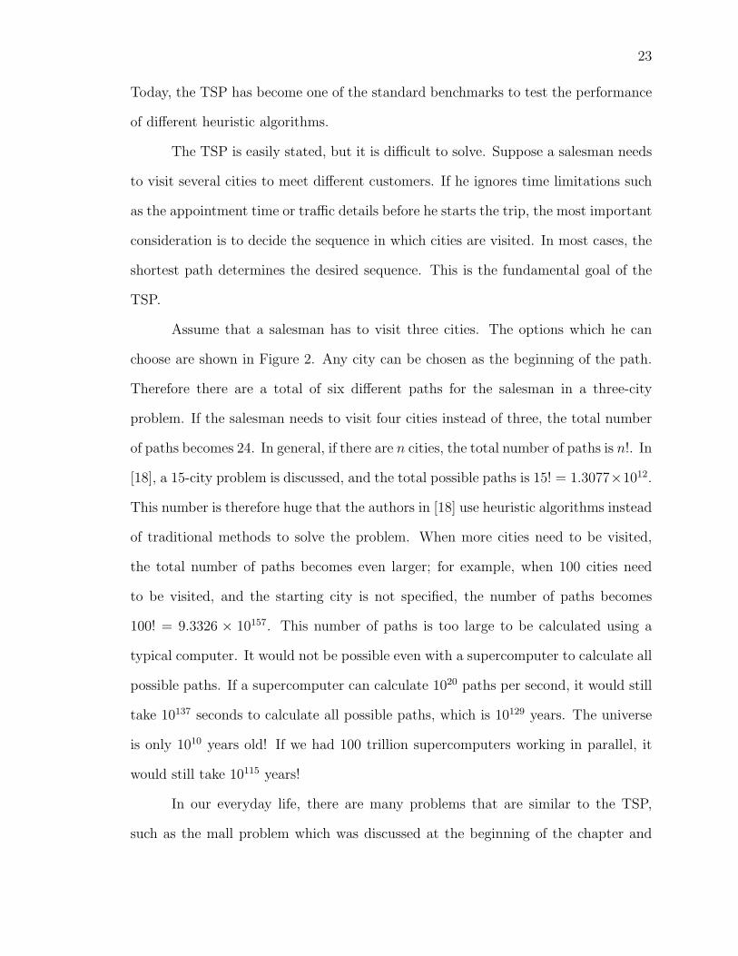
Assume that a salesman has to visit three cities. The options which he can

choose are shown in Figure 2. Any city can be chosen as the beginning of the path.

Therefore there are a total of six different paths for the salesman in a three-city

problem. If the salesman needs to visit four cities instead of three, the total number

of paths becomes 24. In general, if there are n cities, the total number of paths is n!. In

[18], a 15-city problem is discussed, and the total possible paths is 15! = 1.3077×1012.

This number is therefore huge that the authors in [18] use heuristic algorithms instead

of traditional methods to solve the problem. When more cities need to be visited,

the total number of paths becomes even larger; for example, when 100 cities need

to be visited, and the starting city is not specified, the number of paths becomes

100! = 9.3326 × 10157. This number of paths is too large to be calculated using a

typical computer. It would not be possible even with a supercomputer to calculate all

possible paths. If a supercomputer can calculate 1020 paths per second, it would still

take 10137 seconds to calculate all possible paths, which is 10129 years. The universe

is only 1010 years old! If we had 100 trillion supercomputers working in parallel, it

would still take 10115 years!

In our everyday life, there are many problems that are similar to the TSP,

such as the mall problem which was discussed at the beginning of the chapter and

24

Figure 2: The six options for three cities TSP.

25

the mailman problem. Suppose a mailman needs to visit 1000 houses every day.

What is the shortest path? Therefore the TSP is a practical problem which can

be used in many areas, but it is nevertheless a challenge for the traditional solution

methods. For both of these reasons, many heuristic algorithms use the TSP as a

standard benchmark.

3.2 Modification of BBO for the TSP

The TSP is an internally connected problem in the sense that the sequence of

cities (that is, the sequence of SIVs) determines the total distance of a path instead

of the values of SIVs as in a typical BBO problem. The individual SIV does not have

meaning by itself. The SIV in the TSP is a coordinate which only has meaning after

it is assigned a position within a sequence. The sequence of SIVs then determines

the solution to the TSP. In this situation, if we want to immigrate to improve the

fitnesses of the islands, what we need is the information about the sequence of SIVs.

But for the typical BBO algorithm, after the immigration step has been ex-

ecuted, random SIVs from the emigrating island replace random SIVs in the immi-

grating island. As mentioned previously, this kind of immigration is an SIV-based

immigration, not a sequence-based immigration. At this point, the individual SIVs

do not carry any sequence information, therefore the traditional immigration method

in BBO cannot be used in the TSP. The BBO algorithm must be modified according

to a new type of sequence-based immigration which will be discussed in Section 3.2.3.

3.2.1 Parallel Computation

In computer engineering, parallel computation is widely used to solve problems

that take a very long time using only nonparallel computation. The aim of parallel

computation is to divide a huge problem into many small parts and calculate these

26

small parts concurrently on different computers or in different threads [23]. The

advantage of parallel computation is that it can significantly decrease the calculation

time of a problem. In the area of heuristic computation, parallel computation is also

widely used [22]. Problems which need to be solved using heuristic algorithms are

complicated and very hard to solve using traditional methods. Parallel computation

is a good choice for these kinds of problems. In order to use parallel computation,

it is required that the problem can be separated into many parts. A schematic

representation of parallel computation is shown in Figure 3.

Figure 3: Schematic representation of parallel computation with one master station andfour slave stations. The task of the master station is to subdivide the major task intosubtasks, distribute the subtasks to slave stations, and receive results from the slavestations.

In [19], parallel computation is incorporated into the GA. It is not difficult

to combine the GA and parallel computation concepts, resulting in a significant in-

27

crease in the calculation speed. For solution methods which do not involve parallel

computation, the calculations are executed on only one station. When parallel com-

putation is incorporated into BBO, instead of solving the problem using only one

station, the master station distributes the subtasks to the slave stations, and the

actual calculations are executed at the slave stations concurrently. This is similar to

the master-slave system in [20]. The operation steps of parallel computation in a GA

are as follows.

1. Distribute the parameters of the main task from the master station to the slave

stations.

2. Decompose the entire population into sub-populations in the master station.

The number of sub-populations is specific for different problems, and it can be

configured by the user. Each slave station receives a sub-population from the

master station as its own population.

3. Perform crossover and mutation operation at the slave station level.

4. Return fitness values from the slave stations to the master station.

In this section, the master station and slave stations are all virtual stations.

A station can be a CPU, a server, a typical PC, a thread or a supercomputer. With

the development of the Internet, communication among computers is easily achieved.

Parallel computation can also be implemented using Internet, and this provides a

means for parallel computation to share the resources of idle computers connected to

the Internet.

3.2.2 Sequence-based Information Exchange

In order to modify BBO for the TSP using parallel computation, it is necessary

to make a major change in the immigration operation of the BBO. The sequence of

28

the cities determines the fitness of the path. In the TSP, the minimum change that

can be made in a path is to change two SIVs by interchanging two respective cities.

But even with this minimum change, a very large change in the fitness (path length)

can occur.

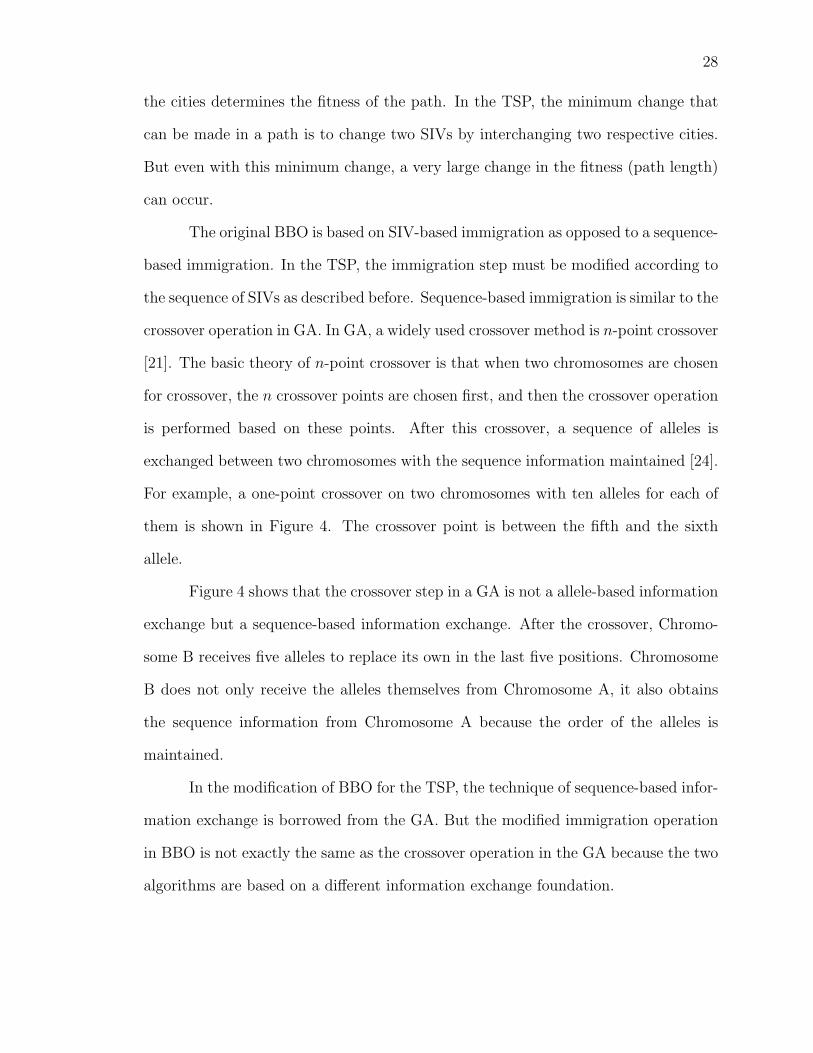
The original BBO is based on SIV-based immigration as opposed to a sequence-

based immigration. In the TSP, the immigration step must be modified according to

the sequence of SIVs as described before. Sequence-based immigration is similar to the

crossover operation in GA. In GA, a widely used crossover method is n-point crossover

[21]. The basic theory of n-point crossover is that when two chromosomes are chosen

for crossover, the n crossover points are chosen first, and then the crossover operation

is performed based on these points. After this crossover, a sequence of alleles is

exchanged between two chromosomes with the sequence information maintained [24].

For example, a one-point crossover on two chromosomes with ten alleles for each of

them is shown in Figure 4. The crossover point is between the fifth and the sixth

allele.

Figure 4 shows that the crossover step in a GA is not a allele-based information

exchange but a sequence-based information exchange. After the crossover, Chromo-

some B receives five alleles to replace its own in the last five positions. Chromosome

B does not only receive the alleles themselves from Chromosome A, it also obtains

the sequence information from Chromosome A because the order of the alleles is

maintained.

In the modification of BBO for the TSP, the technique of sequence-based infor-

mation exchange is borrowed from the GA. But the modified immigration operation

in BBO is not exactly the same as the crossover operation in the GA because the two

algorithms are based on a different information exchange foundation.

29

Figure 4: One-point crossover in GA. Two chromosomes are involved — Chromosome Aand Chromosome B, and the crossover point is between the fifth allele and sixth allele.

3.2.3 BBO/TSP Algorithm

In order to execute the TSP using BBO in a faster way, the parallel compu-

tation and the sequence-based information exchange will be used to modify BBO.

The TSP is very different than other typical optimization problems. For most typical

problems, a SIV can be a random number within its domain. There are an infinite

number of possibilities within the domain of the SIVs. That means an island can

have unique SIVs which do not show up in others, and each island can be a unique

island according to the unique SIVs it has. The aim of BBO when executing this kind

of problem is to find the good SIVs which only appear in some islands, and improve

the fitness of the whole population based on these SIVs.

The TSP is quite different compared to the problem discussed above. The co-

ordinates of the cities are the SIVs for an island, and the cities that will be visited are

known. This means that each island has exactly the same SIVs. The only difference

30

between islands is the sequence of SIVs. Therefore an island does not need to import

an SIV which does not exist in itself to improve its fitness. Also, the traditional

immigration in BBO should be abandoned, because of the fact that the traditional

immigration is based on SIVs rather than the sequence of SIVs.

In the modified BBO, the whole population is only one island, and it already

contains all SIVs needed in the TSP. The goal in the next step is to find the best

sequence of SIVs. Then it is the introduction about how to incorporate the par-

allel computation into BBO. The steps of modified BBO based on sequence-based

immigration and parallel computation are as follows.

1. Decompose the population of the original island into n shares, and send them

to n different sub-islands. Each share is totally different, therefore there is no

duplicated SIVs occurring in sub-islands.

2. Calculate all possible combinations of SIVs in each sub-island, and find out the

best combinations for each sub-island. Then send them back to the original

island.

3. Check all the combinations of sub-populations sent back from sub-islands, and

choose the best one to be the new sequence for the original island. This step is

based on the sequence information of all sub-populations.

4. Based on the performance of each sub-island, operate the immigration step

between different sub-islands. The immigration between sub-islands is based on

roulette wheel just as in original BBO, and the immigration rates and emigration

rates are all determined by the fitness of the sub-islands. Then immigration step

between sub-islands is the same as step 4 and 5 of the original BBO described

in Section 1.1.

31

5. Terminate when satisfying certain criteria for fitness or the maximum generation

is reached. Otherwise, go to step 2 for the next generation.

Figure 5 explains how BBO works with the TSP.

Figure 5: Flow chart for solving the TSP using modified BBO. This flow shows a threesub-islands scenario.

3.3 Simulations

After the modification of BBO based on the TSP, it is the demonstration of the

performance of the modified BBO dealing with a practical problem. In this section,

a 15 cities TSP is used to test the performance of BBO. For a 15 cities TSP, the total

possible combinations are 1.3077×1012, therefore calculating all possible combination

is definitely not a possible solution. Here, two heuristic algorithms are provided to

deal with the TSP — the modified BBO and the GA. The modified BBO is introduced

32

in Section 3.2.3, which is also call BBO/TSP. The GA used in the simulation uses

cycle crossover as its information exchange method.

The cycle crossover is a widely used crossover method in GA, and it can guar-

antee that the offspring is always legal after the crossover [25]. The following example

shows how cycle crossover works. An offspring needs two parents, and the parents

are shown in Figure 6.

Figure 6: Two parents of an offspring. A — G are seven different alleles in the chromo-somes.

First, the allele in the first position of chromosome 1 is picked as the allele in

the first position of offspring chromosome. Here, E is chosen as the allele in the first

position of the offspring chromosome, as shown in Figure 7.

Figure 7: The first step in cycle crossover.

Second, the first chosen allele is E, and the position of allele E is 1. In chro-

mosome 2, allele C is in position 1, therefore C is chosen as another allele in the

offspring chromosome. The position of allele C in the offspring chromosome is the

33

same as the position of allele C in chromosome 1. Therefore the position of allele C

in the offspring chromosome is 7, as shown in Figure 8.

Figure 8: The second step in cycle crossover.

Third, repeat the method in the second step. The position of allele C in

chromosome 1 is 7, and allele G is in the same position in chromosome 2. The

position of G in chromosome 1 is 5, therefore the position of allele G in the offspring

chromosome is 5. Following this method, the position of allele A in the offspring

chromosome can be found next, as shown in Figure 9.

Figure 9: The third step in cycle crossover.

When the position of allele A in the offspring chromosome is determined, allele

E is chosen to determine its position in the offspring chromosome. But the position

of allele E has already been determined, and the chosen alleles become a cycle at

34

this time. This is where the name cycle crossover comes from. For the unchosen

alleles, their positions in the offspring are the same as in chromosome 2. After that,

all the positions of alleles are determined, and the offspring chromosome is complete,

as shown in Figure 10.

Figure 10: The final step in cycle crossover.

3.3.1 Parameter Specifications

The coordinates of 15 cities are shown in Table V. These coordinates were

specifically chosen to be scattered in a non-uniform way in two dimensions. In addi-

tion, this problem has the characteristic that inter-city distances widely vary. There-

fore, this problem provides a good TSP benchmark.

Table V: The coordinates of 15 cities.City 1 City 2 City 3 City 4 City 5

Coordinates (120,36) (22,10) (219,11) (2,60) (30,144)

City 6 City 7 City 8 City 9 City 10Coordinates (350,199) (156,78) (167,79) (289,142) (48,300)

City City 11 City 12 City 13 City 14 City 15Coordinates (231,182) (333,222) (123,321) (56,45) (67,86)

The BBO parameters are as follows:

35



• Number of sub-islands: 5

• Number of SIVs in each sub-island: 3

• Generations: 1000

• Mutation rate: 0


The GA parameters are as follows:

• Number of chromosomes: 10

• Number of alleles per chromosome: 15

• Generations: 1000

• Mutation rate: 0


3.3.2 Simulation Results and Analysis

After the parameter specifications of both BBO/TSP and GA, these two al-

gorithms are used to solve the 15 cities TSP. The TSP results of the BBO/TSP and

GA are shown in Table VI.

The following are the two best sequences of cities achieved by BBO/TSP and

GA after 100 Monte Carlo simulations. The best sequence achieved by BBO is City

36

Table VI: Results of the TSP using BBO/TSP and GA.BBO/TSP GA

Best path distance 1.1186× 103 1.3874× 103

12, 6, 9, 11, 7, 3, 8, 1, 14, 4, 2, 15, 5, 10, 13. The best sequence achieved by GA is

City 6, 9, 12, 11, 13, 10, 5, 4, 2, 15, 7, 1, 14, 3, 8. Figure 11 and Figure 12 show the

shorest paths in the coordinate map.

Figure 11: Best sequence of 15 cities achieved by BBO/TSP.

From the results shown in Table VI, the shortest path achieved by BBO/TSP

is 1.1186 × 103, and the shortest path achieved by GA is 1.3874 × 103. The result

achieved by BBO/TSP is 24% better than GA. Therefore BBO/TSP outperforms

GA when dealing with the TSP. Another attraction of this simulation is that the

calculation times used by BBO/TSP and GA are both less than four seconds. As you

can see, BBO/TSP also has good time efficiency.

37

Figure 12: Best sequence of 15 cities achieved by GA.

CHAPTER IV

MODIFICATION OF BBO BASED ON

KALMAN FILTER FOR NOISY

ENVIRONMENTS

In this chapter, the main focus is how to operate BBO in a noisy environment.

In Section 4.1, it is about the detrimental effect of noise. In Section 4.2, it is the

introduction about the history and theory of the Kalman filter. In Section 4.3, it is

about how to calculate the probability that two fitnesses switch their positions due to

the effect of noise. In Section 4.4, it is the contribution of a single SIV to the fitness

of the entire island. In Section 4.5, it is the introduction about the three options

in the immigration step. In the last section, it shows the simulation results and the

analysis of different BBOs.

38

39

4.1 Detrimental Effect of Noise

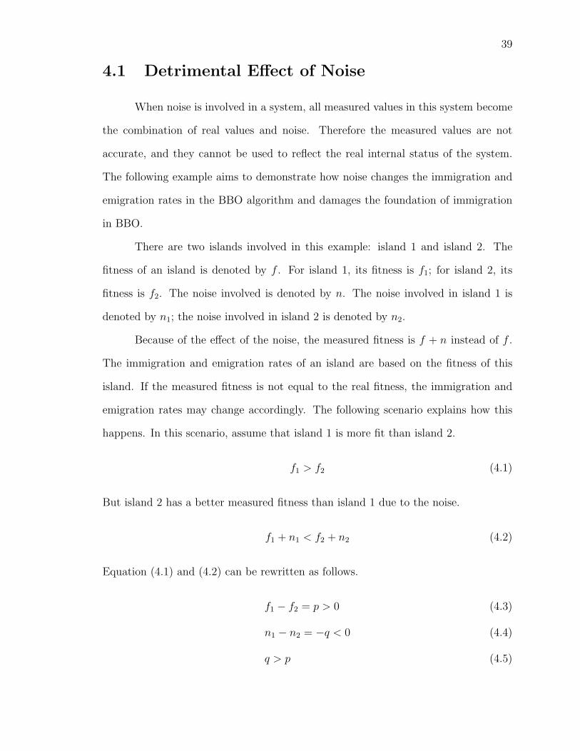
When noise is involved in a system, all measured values in this system become

the combination of real values and noise. Therefore the measured values are not

accurate, and they cannot be used to reflect the real internal status of the system.

The following example aims to demonstrate how noise changes the immigration and

emigration rates in the BBO algorithm and damages the foundation of immigration

in BBO.

There are two islands involved in this example: island 1 and island 2. The

fitness of an island is denoted by f . For island 1, its fitness is f1; for island 2, its

fitness is f2. The noise involved is denoted by n. The noise involved in island 1 is

denoted by n1; the noise involved in island 2 is denoted by n2.

Because of the effect of the noise, the measured fitness is f + n instead of f .

The immigration and emigration rates of an island are based on the fitness of this

island. If the measured fitness is not equal to the real fitness, the immigration and

emigration rates may change accordingly. The following scenario explains how this

happens. In this scenario, assume that island 1 is more fit than island 2.

f1 > f2 (4.1)

But island 2 has a better measured fitness than island 1 due to the noise.

f1 + n1 < f2 + n2 (4.2)

Equation (4.1) and (4.2) can be rewritten as follows.

f1 − f2 = p > 0 (4.3)

n1 − n2 = −q < 0 (4.4)

q > p (4.5)

40

When the fitnesses of islands are sorted in ascending order, the positions of these two

fitnesses are switched because of noise. In BBO, the immigration and emigration rates

are assigned to different islands according to the fitness of each island. If the noise

has a strong effect on the fitnesses of islands, the sequence of the measured fitnesses

could be much different from the sequence of the true fitnesses. An island with good

performance may get a low emigration rate and high immigration rate, and an island

with poor performance may get a high emigration rate and low immigration rate.

This is the opposite of what the true immigration and emigration rates ought to be.

Therefore the immigration and emigration rates do not reflect the fitness of an island.

This means in the immigration part of BBO, an island with poor performance may

get a greater chance to emigrate its SIVs to other islands compared to an island with

good performance. If this happens, the immigration mechanism of BBO is corrupted,

and BBO will not perform as well as in a noiseless environment.

4.2 The Kalman Filter

The theory of the Kalman filter was invented by R. Kalman in 1960 [26]. It

is a recursive filter which can estimate states in a noisy environment [27]. In the

past 50 years, the contribution of the Kalman filter in noisy environments has been

significant, and it has become the theoretical foundation of many famous applications,

for example, navigation systems [28].

One of the most important contributions of the Kalman filter is that it can

make an estimation of the true state value in a noisy environment. In the BBO

problem, each fitness is the sum of the true fitness and a random noise. Therefore

the measured fitnesses are not equal to the true fitnesses. According to Section 4.1,

the detrimental effect of noise is that it changes the true emigration and immigration

rates of each island. The Kalman filter provides a better estimate of the true fitnesses

41

of the islands compared to the measured ones.

In this application of the Kalman filter to BBO, noise was added only to the

fitness measurement, and this is called the observation noise. No noise was added to

the system process. Each fitness is a scalar, therefore the Kalman filter only needs

to estimate a scalar for each island, not a vector. In this case, the Kalman filter is

simplified to a scalar version [29], which reduces the complexity of the calculation

compared to the vector version of the Kalman filter [30]. The formulation of the

scalar Kalman filter is as follows.

P = Pprior +Q (4.6)

m = mprior +Pprior

Pprior +R(g −mprior) (4.7)

P =PpriorR

Pprior +R(4.8)

where P is the uncertainty of the state estimate, m is the estimated fitness, g is the

measured fitness, Q is the variance of the process noise, and R is the variance of the

observation noise. The uncertainty Pprior and the estimated fitness mprior are the

values from the previous iteration step before the most recent fitness measurement

is updated. The process noise is assumed to be zero, therefore the uncertainty P is

only related to Pprior and R. Equation (4.8) can be rewritten as follows.

P =PpriorR

Pprior +R

=Pprior

Pprior

R+ 1

(4.9)

BecausePprior

R> 0, we see that

Pprior

R+ 1 > 1. Therefore

PpriorPprior

R+1

< Pprior. With each

step in the Kalman algorithm, the uncertainty P will be reduced according to R and

Pprior. With smaller uncertainty, the estimation of the fitness is more accurate. In

the limit as the number of measurements approaches infinity, the Kalman filter gives

an estimate of the fitness which is equal to the true value.

42

A disadvantage of the Kalman filter is that it needs the measured fitness g for

the calculation of the uncertainty at every step, which increases the cost of calculation.

For many practical optimization problems, a call to the cost function requires a long

calculation time. Therefore the question is: how many times should the Kalman filter

be called in BBO before performing a migration? The question may be answered by

using a probabilistic argument to optimize the advantage of the Kalman filter over

its disadvantages.

4.3 Probability Calculations

According to Section 4.2, the sequence of the measured fitnesses is different

from the true fitnesses due to the effect of noise, therefore the immigration mechanism

of BBO is damaged. In this section, different scenarios are introduced, and the

probability that two fitnesses switch positions in each scenario is calculated.

4.3.1 Global Probability of Island-Switching

First, it is a simple scenario. For two islands which switch fitness positions

with each other, suppose they have the same fitness range and noise range. The

fitness range is [v − a, v + a], a ∈ [0,∞) as shown in Figure 13. The noise range is

[−b, b], b ∈ [0,∞) as shown in Figure 14. Both the fitness and the noise are uniformly

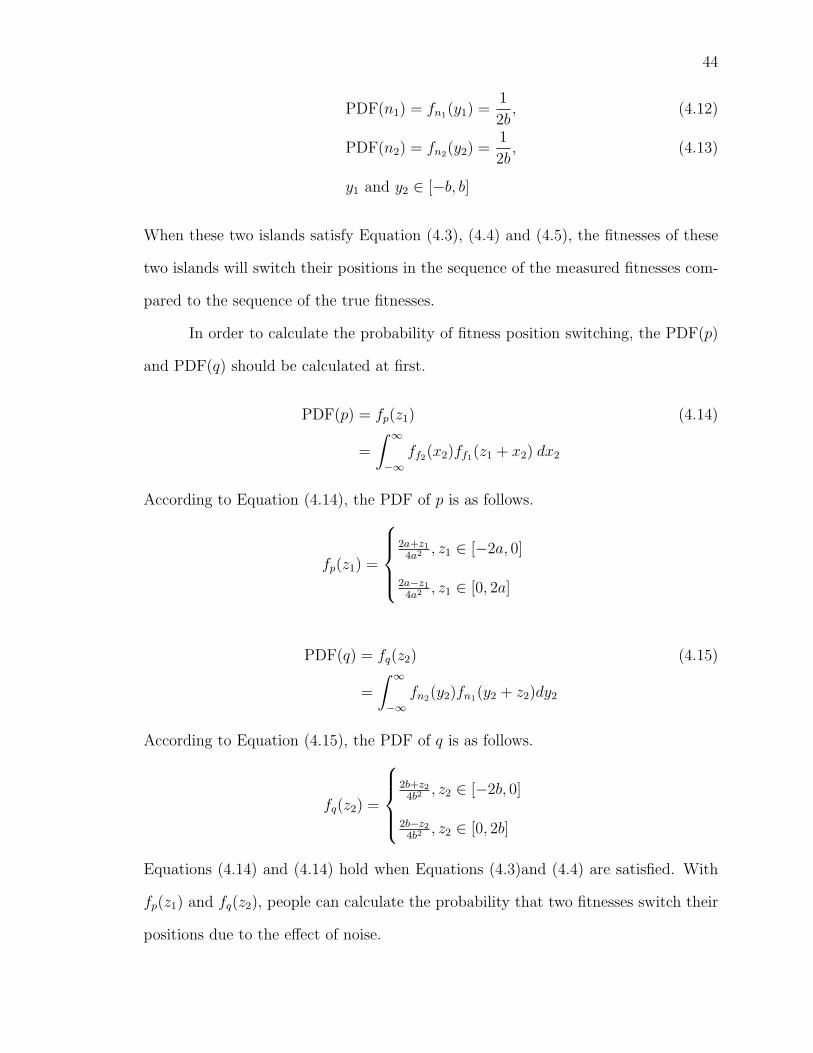
distributed. The PDF of the fitness of an island and the noise are as follows.

PDF(f1) = ff1(x1) =1

2a, (4.10)

PDF(f2) = ff2(x2) =1

2a, (4.11)

x1 and x2 ∈ [v − a, v + a]

43

Figure 13: The PDF of the fitness of an island.

Figure 14: The PDF of noise involved in the fitness.

44

PDF(n1) = fn1(y1) =1

2b, (4.12)

PDF(n2) = fn2(y2) =1

2b, (4.13)

y1 and y2 ∈ [−b, b]

When these two islands satisfy Equation (4.3), (4.4) and (4.5), the fitnesses of these

two islands will switch their positions in the sequence of the measured fitnesses com-

pared to the sequence of the true fitnesses.

In order to calculate the probability of fitness position switching, the PDF(p)

and PDF(q) should be calculated at first.

PDF(p) = fp(z1) (4.14)

=

∫ ∞

−∞ff2(x2)ff1(z1 + x2) dx2

According to Equation (4.14), the PDF of p is as follows.

fp(z1) =

2a+z14a2 , z1 ∈ [−2a, 0]

2a−z14a2 , z1 ∈ [0, 2a]

PDF(q) = fq(z2) (4.15)

=

∫ ∞

−∞fn2(y2)fn1(y2 + z2)dy2

According to Equation (4.15), the PDF of q is as follows.

fq(z2) =

2b+z24b2

, z2 ∈ [−2b, 0]

2b−z24b2

, z2 ∈ [0, 2b]

Equations (4.14) and (4.14) hold when Equations (4.3)and (4.4) are satisfied. With

fp(z1) and fq(z2), people can calculate the probability that two fitnesses switch their

positions due to the effect of noise.

45

When a > b we obtain:

P (switch) = P (q > p) (4.16)

=

∫ 2b

0

∫ z2

0

fp(z1)fq(z2)dz1 dz2

=b(−b+ 4a)

24a2

When a < b we obtain:

P (switch) = P (q > p) (4.17)

=

∫ 2a

0

∫ z2

0

fp(z1)fq(z2)dz1 dz2+∫ 2b

2a

∫ 2a

0

fp(z1)fq(z2)dz1 dz2

=a2

24b2− a

6b+

1

4

With these calculation results, even before doing any further simulation step,

the probability of fitness position switching can be found. But the scenario discussed

above is quite simple, especially the fact that the range of noise is the same for every

island. For the Kalman filter, its aim is to reduce the effect of noise. Therefore after

one Kalman filter step, some islands will be re-evaluated, and the ranges of the noises

in the corresponding islands will change accordingly. If each island has different noise

ranges, the probabilities calculated above cannot be used. Here, different noise ranges

for different islands will be used, then the probabilities of fitness position switching

will be calculated again. In this calculation, there are two noises with different ranges

involved. n1 is the noise involved in the first island. n2 is the noise involved in the

second island. They are still uniformly distributed. The PDF of n1 and n2 are as

follows.

PDF(n1) = fn1(y1) =1

2b, y1 ∈ [−b, b] (4.18)

PDF(n2) = fn2(y2) =1

2c, y2 ∈ [−c, c] (4.19)

46

Figure 15: The PDF of noises with different ranges, when b > c.

Figure 16: The PDF of noises with different ranges, when c > b.

47

With the change of fn1(y1) and fn1(y1), fq(z2) should be recalculated.

When b > c we obtain:

fq(z2) =

12b, z2 ∈ [0, b− c]

b+c−z24bc

, z2 ∈ [b− c, b+ c]

When b < c we obtain:

fq(z2) =

12c, z2 ∈ [0, c− b]

b+c−z24bc

, z2 ∈ [c− b, c+ b]

With fp(z1) and fq(z2), the probability of fitness position switching with the noises

which have different ranges can be calculated. Equation (4.16) and (4.17) are modified

as follows.

When 2a > b+ c and b ≥ c we obtain:

P (switch) = P (q > p) (4.20)

=

∫ b−c

0

∫ z2

0

fp(z1)fq(z2)dz1 dz2+∫ b+c

b−c

∫ z2

0

fp(z1)fq(z2)dz1 dz2

=−b3 − bc2 + 6ab2 + 2ac2

48a2b

When 2a > b+ c and b < c we obtain:

P (switch) = P (q > p) (4.21)

=

∫ b−c

0

∫ z2

0


b−c

∫ z2

0

fp(z1)fq(z2)dz1 dz2

=−b2c− c3 + 2ab2 + 6ac2

48a2c

48

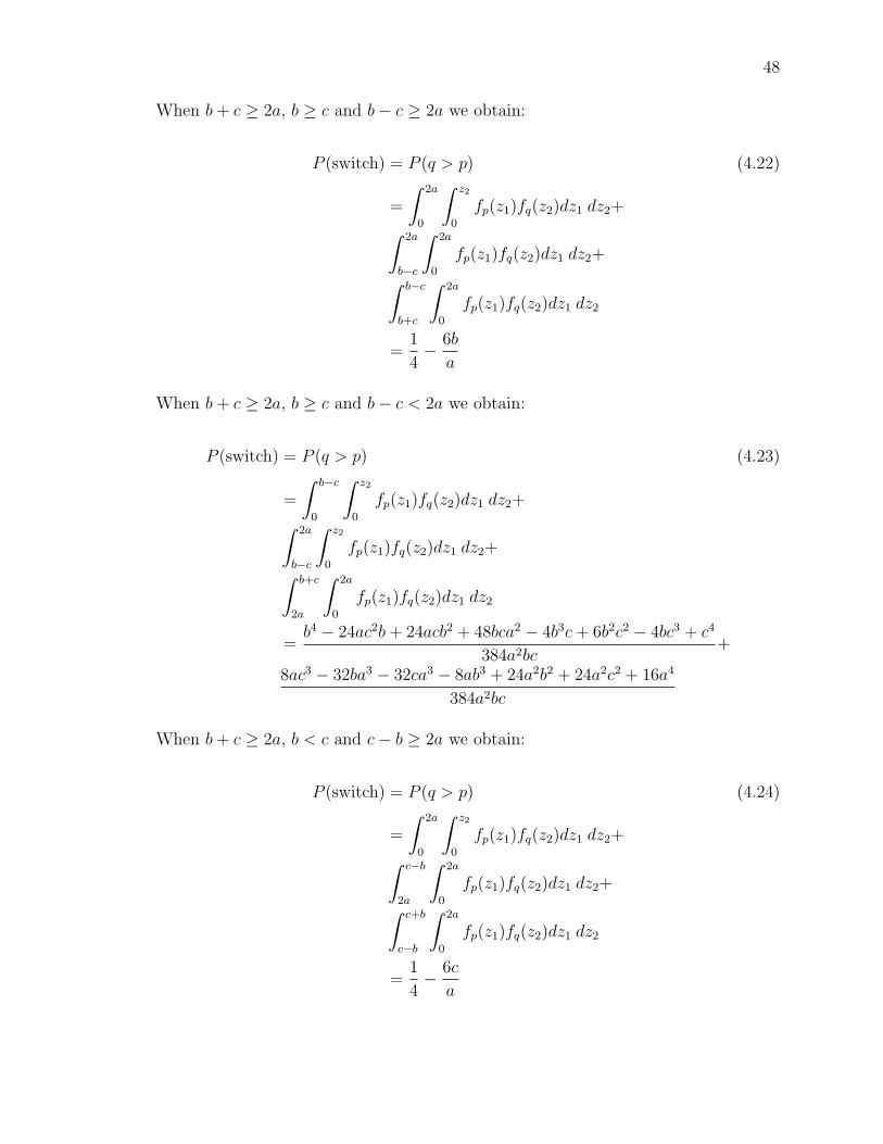
When b+ c ≥ 2a, b ≥ c and b− c ≥ 2a we obtain:

P (switch) = P (q > p) (4.22)

=

∫ 2a

0

∫ z2

0

fp(z1)fq(z2)dz1 dz2+∫ 2a

b−c

∫ 2a

0

fp(z1)fq(z2)dz1 dz2+∫ b−c

b+c

∫ 2a

0

fp(z1)fq(z2)dz1 dz2

=1

4− 6b

a

When b+ c ≥ 2a, b ≥ c and b− c < 2a we obtain:

P (switch) = P (q > p) (4.23)

=

∫ b−c

0

∫ z2

0


b−c

∫ z2

0


2a

∫ 2a

0

fp(z1)fq(z2)dz1 dz2

=b4 − 24ac2b+ 24acb2 + 48bca2 − 4b3c+ 6b2c2 − 4bc3 + c4

384a2bc+

8ac3 − 32ba3 − 32ca3 − 8ab3 + 24a2b2 + 24a2c2 + 16a4

384a2bc

When b+ c ≥ 2a, b < c and c− b ≥ 2a we obtain:

P (switch) = P (q > p) (4.24)

=

∫ 2a

0

∫ z2

0

fp(z1)fq(z2)dz1 dz2+∫ c−b

2a

∫ 2a

0

fp(z1)fq(z2)dz1 dz2+∫ c+b

c−b

∫ 2a

0

fp(z1)fq(z2)dz1 dz2

=1

4− 6c

a

49

When b+ c ≥ 2a, b < c and c− b < 2a we obtain:

P (switch) = P (q > p) (4.25)

=

∫ 0

c−b

∫ z2

0


c−b

∫ z2

0

fp(z1)fq(z2)dz1 dz2+∫ c+b

2a

∫ 2a

0

fp(z1)fq(z2)dz1 dz2

=b4 + 24ac2b− 24acb2 + 48bca2 − 4b3c+ 6b2c2 − 4bc3 + c4

384a2bc+

−8ac3 − 32ba3 − 32ca3 + 8ab3 + 24a2b2 + 24a2c2 + 16a4

384a2bc

In summary, there are six different scenarios. P (switch) is as follows.

P (switch) =

−b3−bc2+6ab2+2ac2

48a2b, if 2a > b + c and b ≥ c;

−b2c−c3+2ab2+6ac2

48a2c, if 2a > b + c and b < c;

14− 6b

a, if b + c ≥ 2a, b ≥ c and b− c ≥ 2a;

b4−24ac2b+24acb2+48bca2−4b3c384a2bc

+6b2c2−4bc3+c4+8ac3−32ba3−32ca3

384a2bc

+−8ab3+24a2b2+24a2c2+16a4

384a2bc, if b + c ≥ 2a, b ≥ c and b− c < 2a;

14− 6c

a, if b + c ≥ 2a, b < c and c− b ≥ 2a;

b4+24ac2b−24acb2+48bca2−4b3c384a2bc

+−4bc3+c4−8ac3−32ba3−32ca3

384a2bc

+6b2c2+8ab3+24a2b2+24a2c2+16a4

384a2bc, if b + c ≥ 2a, b < c and c− b < 2a.

After the calculations, probability that two fitnesses switch their positions even before

the migration step in BBO can be found. This offers a good theoretical support to

help users make the right decision in the migration step. In many heuristic problems,

cost functions are long and complicated, and it takes a long time for calculation. With

50

the help of these probabilities, we can effectively avoid most unnecessary immigrations

caused by noise. Therefore the benefit of these probabilities is that their use can save

unnecessary calculation time for the BBO algorithm.

4.3.2 Local Probability of Islands Switching

In Section 4.3.1, the calculated probability is called the global probability.

Since the islands involved in the calculation are two random ones within the domain,

these probabilities are based on all possible pairs of islands in the population. Ac-

cording to these probabilities, users can make their own decisions in the migration

step: finish the immigration, refuse the immigration, or re-evaluate the fitnesses of

the islands. But the global probability only provides a general guideline for users.

Because the global probability is based on the entire population, it is like an expected

probability of fitness position switching. In the real migration step, there are only

two islands involved: the selected immigrating island and the selected emigrating

island. In other words, the global probability of islands position switching can only

provide users the general direction in the migration step. If users require more accu-

rate probabilities for each migration step, it is necessary to calculate the probability

of fitness position switching for each specific migration. This probability of fitness

position switching for each specific immigration step is called the local probability of

islands switching.

In BBO with the Kalman filter incorporated, the immigrating island only re-

ceives immigration from an emigrating island that has a better fitness. Suppose there

are two islands: island 1 and island 2. When noise is combined with the fitnesses,

there is some chance that the real fitness of island 1 is better than the island 2, but the

measured fitness of island 1 is always worse than island 2. If this scenario happens,

and island 1 receives immigration from island 2, there is a chance to ruin the fitness

51

of island 1. Therefore the aim of probability calculation is to prevent this situation.

Figure 17, Figure 18, Figure 19 and Figure 20 show PDFs of the immigrating island

and the emigrating island in four scenarios.

Figure 17: The PDFs of the measured fitnesses of the immigrating island and the emi-grating island in scenario 1. F1 is the measured fitness of the immigrating island, and F2is the measured fitness of the emigrating island. U1 is the uncertainty in the fitness ofthe immigrating island, and U2 is the uncertainty in the fitness of the emigrating island.

52



53


P (switch) in the four scenarios is as follows.

P (switch) =

∫ F1+U1

F2−U2

∫ F1+U1

f2

12U1

12U2

df1df2,

Scenario 1 (Figure 17);

0,


∫ F2+U2

F2−U2

∫ F2+U2

f2

12U1

12U2

df1df2 +∫ F1+U1

F2+U21

2U1df1df2,


∫ F1+U1

F1−U1

∫ F1+U1

f2

12U1

12U2

df1df2 +∫ F1−U1

F2−U21

2U2df1df2,

Scenario 4 (Figure 20).

Users can calculate P (switch) for two specific islands in every migration step. This

54

can provide more accurate probability to help users make decisions before migration.

With P (switch), users can avoid undesirable immigration and significantly decrease

the calculation time for problems with complicated cost functions..

4.4 The Fitness Contribution of a Single SIV

The fitness of an island is based on the performance of its SIVs. In this section,

it is about the contribution of one SIV to the fitness of an island. Suppose there are

two islands: the immigrating island and the emigrating island. f represents the

fitness of an island. Therefore the fitness of the immigrating island is called f1, and

the fitness of the emigrating island is called f2. The number of SIVs in each island is

s.

Cost functions used in heuristic computation are often sophisticated, and not

all the cost functions can be separated by SIV. Therefore the exact contribution of

each SIV to the fitness is not an exact number but a range. For a single SIV, the

average range of its contribution to the fitness is as follows [32].

Contribution of one SIV = CS ∈

[f

s− d

√3

s,f

s+ d

√3

s

]. (4.26)

Here, the PDF of the contribution of a single SIV is assumed to be uniformly dis-

tributed, where d is the standard deviation of the fitnesses of all islands.

d =√E(f 2)− [E(f)]2 (4.27)

The SIV from the emigrating island is called iSIV; the replaced SIV in the immigrating

island is called rSIV. The ranges of fitness contributions of rSIV and iSIV are as

follows, and they are both uniformly distributed.

Fitness contribution of rSIV ∈[f1s− d

√3s, f1s

+ d√

3s

],

Fitness contribution of iSIV ∈[f2s− d

√3s, f2s

+ d√

3s

].

55

In order to improve the fitness of the immigrating island, the immigrated SIV should

have a better contribution to the fitness than the replaced SIV, which is equivalent to

saying that iSIV should be bigger than rSIV. Figures 21—24 show the four possible

relationships of iSIV and rSIV.

Figure 21: The PDFs of the fitness contribution of iSIV and rSIV in scenario 1.


In general, the probability for each specific case should be calculated. But the

optimization environment is noisy. Therefore the measured fitness is the combination

of the true fitness and the noise. It is not practical to calculate the contribution of each

SIV based on the measured fitness, because in general, the functional form of the cost

function is not known. In this situation, instead of calculating the specific probability

56



57

for each case, the global probability is used. According to the four relationships shown

in Figures 21—24, the probability that the fitness contribution of rSIV is bigger than

the fitness contribution of iSIV is calculated, which is denoted as P (rSIV>iSIV).

f1,t is the real fitness of the immigrating island in the current generation,

and f1,t+1 is the real fitness of the immigrating island in the next generation after

immigration. f2 is the real fitness of the emigrating island in the current generation.

m1,t is the estimate of the fitness of the immigrating island in the current generation.

m2 is the estimate of the fitness of the emigrating island in the current generation.

The probability that immigration will improve the fitness of the immigrating island

can be calculated using the results of the previous section, and using the assumptions

for fitness contribution in this section.

In order to calculate the probability of improvement, Baye’s rule [31] is used

to write:

P (f1,t+1 > f1,t|f2 > f1,t) = P (iSIV > rSIV|f2 > f1,t) (4.28)

=P (iSIV > rSIV, f2 > f1,t)

P (f2 > f1,t)

=P (iSIV > rSIV, f2 > f1,t)

P (f2 > f1,t|m2 > m1,t) + P (f2 > f1,t|m2 < m1,t)

Now notice that m2 will always be greater than m1,t. This is because the Kalman-

assisted BBO algorithm is defined such that the immigrating island will always choose

to immigrate from an island which has an estimated fitness better than itself. There-

fore,

P (f1,t+1 > f1,t|f2 > f1,t) =P (iSIV > rSIV, f2 > f1,t)

P (f2 > f1,t|m2 > m1,t)(4.29)

Looking at the right side of Equation (4.29), P (iSIV > rSIV, f2 > f1,t) can be cal-

culated using one of Figures 21—24, along with the assumed knowledge of the PDFs

of the fitness contributions of iSIV and rSIV. The other term on the right side of

Equation (4.29), P (f2 > f1,t|m2 > m1,t), is simply equal to (1 − P (switch)), where

58

P (switch) is given at the end of the previous section, and which depends on the PDFs

of f1,t and f2.

In a similar way, people can obtain

P (f1,t+1 > f1,t|f2 < f1,t) =P (iSIV > rSIV, f2 < f1,t)

P (f2 < f1,t|m2 > m1,t)(4.30)

Now the results of Equation (4.29) and (4.30) are used, along with Baye’s rule, to

calculate

P (f1,t+1 > f1,t) = P (f1,t+1 > f1,t|f2 > f1,t) + P (f1,t+1 > f1,t|f2 < f1,t) (4.31)

In summary, given two island fitness values, Equation (4.31) gives the probability

that an immigration from the emigrating island will result in an improvement in the

fitness of the immigrating island.

4.5 Three Immigration Options

Based on Section 4.4, the probability that the fitness of the immigrating island

gets improved after one generation can be found. In this section, three options are

set in the immigration step to find the balance for how many times the Kalman filter

should be used in BBO.

4.5.1 Option One: No Island Re-evaluation

In the first option, there are two islands involved: the immigrating island and

the emigrating island. In the immigration step, each immigrating island can only

receive one immigrated SIV from the emigrating island in one generation. Here, the

immigrating island is called island 1, and the emigrating island is called island 2.

In option one, first, two clones of island 1 are made, island 1a and island

1b. Second, island 1a receives an immigrated SIV from island 2. Third, island 1b

59

receives an immigrated SIV from island 2. After that, both island 1a and island 1b

get evaluated, and the one which has the higher measured fitness is chosen to be

island 1 in the next generation. The probability that either island 1a or island 1b has

a better fitness than the original island 1 is as follows.

Poption1 = 1− (1− P (f1a,t+1 > f1a,t))(1− P (f1b,t+1 > f1b,t)) (4.32)

= 1− (1− P (f1,t+1 > f1,t))2

where the probability on the right side of the equation is given in Equation (4.31).

4.5.2 Option Two: Immigrating Island Re-evaluation

In the second option, there are two islands involved, the immigrating island and

the emigrating island. This scenario has similar points with the option one because

one SIV immigration is also used in this option.

According to Equation (4.9), each time the Kalman filter is used to re-evaluate

the island, the uncertainty of the re-evaluated island will get decreased accordingly.

At the same time, P (switch) is decided by the measured fitnesses and the uncertainties

of the immigrating island and the emigrating island.

In option two, first, in order to decrease the uncertainty of immigrating island,

immigrating island is re-evaluated. Even before re-evaluating the immigrating island,

the new uncertainty can be calculated according to Equation (4.8). The expected

measured fitness after re-evaluation is the same as the one before re-evaluation. That

means that without any cost function calculation, the new P (switch) for the emigrat-

ing island and the re-evaluated immigrating island can be found.

Poption2 = Pnew(f1,t+1 > f1,t) (4.33)


When the immigrating island is re-evaluated, the estimation of the fitness of the im-

60

migrating island will change accordingly. In the probability calculation, the expected

estimated fitness is used. But the new estimation of the fitness is not equal to the

expected one; it can be either better or worse. If the new estimation of the fitness of

the immigrating island is still worse than the emigrating island, the emigrating island

immigrates an SIV to the immigrating island; if the new estimation of the fitness of

the immigrating island is better than the emigrating island, the island that had been

chosen for immigration is re-evaluated instead of finishing the immigration step.

4.5.3 Option Three: Emigrating Island Re-evaluation

In the third option, most of the steps are the same as in option two. The

only difference is that instead of re-evaluating the immigrating island, the emigrating

island is chosen to be re-evaluated at first.

First, calculate the new P (switch) under the condition that the emigrating

island is re-evaluated.

Poption3 = Pnew(f1,t+1 > f1,t) (4.34)


Second, if the new estimated fitness of emigrating island is still better than

the immigrating island, the emigrating island immigrates an SIV to the immigrating

island; on the other hand, if the new estimated fitness of the emigrating island is

worse than the immigrating island, the emigrating island is re-evaluated instead of

doing immigration.

4.5.4 Optimal Option Selection

When the three options are defined for the immigration step, how to choose

the option becomes another question. Because of the noise, the measured fitness of

61

each island is not accurate. It is hard to confidently depend on the accuracy of the

measured fitness in the immigration step. Therefore the improvement probability

(the probability that the immigrating island will get improved) is used to be the

criteria of choosing the desired option. Figure 25 shows the operating diagram in the

immigration step.

Figure 25: The three options in the immigration step — no re-evaluation option, immi-grating island re-evaluation option, and emigrating island re-evaluation option.

In my problem, a fair comparison is necessary. Each call of the cost function

can result in extensive calculations. If the three options have different costs, the

comparison among them is unfair. In order to avoid unfair comparison for these

three options, each option requires the same number of calls of the cost function.

For the first option, the immigrating island has two chances to improve its

fitness since two SIV immigrations are performed, and two calls of the cost function

are used in this option.

For the second option, the Kalman filter part uses one call of the cost function

62

at first. If the immigration is accepted by the immigrating island, another call of

the cost function is used to evaluate the new immigrating island. If immigration is

denied, the immigrating island is re-evaluated based on the Kalman filter, and it uses

one call of the cost function. Therefore in option two, two calls of the cost function

are used.

In option three, similar to option two, the Kalman filter part uses one call of

the cost function at first. If the immigration is accepted by the immigrating island,

another call of the cost function is used to evaluate the new immigrating island. If

immigration is denied, the emigrating island is re-evaluated based on the Kalman

filter, and it uses one call of the cost function. Therefore in option three, two calls of

the cost function are used.

For each of three options, two calls of the cost function are used. Therefore

the comparison among them is a fair one.

4.6 Simulations

MATLAB R© is used as the simulation environment. Three types of BBOs

are used to test performance. The first BBO is the modified BBO based on the

Kalman filter and probabilities calculation, which is called KBBO. The second BBO

is the basic BBO, which is called RBBO (regular BBO). The third BBO is the basic

BBO without noise involved, which is called NBBO. For the first two BBOs, the

optimization environment is noisy. For the last one, the optimization environment is

noiseless.

4.6.1 Parameter Specifications

The main parameters used in the BBOs are as follows:

63




• Mutation probability: 0.005

• Elitism parameter: 0

For all three BBOs, the immigration step only performs one SIV immigration

as in Section 4.5. The cost function is shown as follows.

fitness = ((x21 + x2

2 + 100)14 − 3.6552)× 10, x1, x2 ∈ [0, 10] (4.35)

In the cost function, x1 is the first SIV of the island and x2 is the second SIV of the

island. The range of the SIVs is [0,10]. The range of fitnesses is [−4.9291, 5.0659].

The range of the fitness measurement noise is [−5, 5].

4.6.2 Simulation Results and Analysis

In heuristic algorithms, the performance of each island is determined by the

fitness value. The final aim of all heuristic algorithms is to improve the performance

of all islands, or the best island generation by generation. Therefore there are two

common methods that can be use as the criteria when comparing the performances

of different heuristic algorithms: comparing the best fitness and comparing the mean

fitness.

For some problems, the only useful island is the island which has the best

fitness. For example, in the TSP, the island with the shortest path is the final solution,

and the use of the other islands is to provide diversity for the entire population. But

for other problems, the performance of all islands should be considered such as when

a user is interested in finding a highly diverse set of good solutions to some problem.

64

In my simulation, in order to make a fair comparison with all BBOs, both the

best fitness and the mean fitness of all islands are compared. Also, 100 Monte Carlo

simulations are run for each BBO, which increases the fairness of the comparison.

First, consider the comparison based on the best fitness of the islands. For

each generation, the best fitness of the islands is plotted from all 100 Monte Carlo

simulations as shown in Figure 26. All of BBOs achieve the best fitness within 50

calls of the cost function. Even BBO without any modification achieves the goal very

fast. This shows that BBO has a certain tolerance for noise. But there are still some

differences among the different BBOs. Though all BBOs achieve the best fitness, the

improvement speed of each BBO is different. Among BBOs, the improvement speed

of NBBO is fastest. For the maximum value searching problem, the performance of

KBBO is not as good as the other two BBOs.

Figure 26: The maximum fitnesses of RBBO, KBBO and NBBO after 100 Monte Carlosimulations.

Second, all BBOs are compared based on the mean fitness of all islands in each

generation. The mean fitness means averaging all the fitnesses in each generation over

100 Monte Carlo simulations. Figure 27 shows the mean fitness values of all BBOs.

65

Figure 27: The mean fitnesses of RBBO, KBBO and NBBO after 100 Monte Carlosimulations.

All three BBOs achieve their own best mean fitness after about 150 calls of

cost function. While the levels of the mean fitnesses are quite different, all three

fitnesses stay steady at different levels. Compared to KBBO and NBBO, the steady

mean fitness of RBBO is much lower. Although the improvement speed of KBBO

is slower than NBBO and RBBO, the steady mean fitness of KBBO is even better

than NBBO, which does not even involve any noise in the environment. Therefore the

Kalman-based modification of BBO provides a good performance solution when mean

fitness is the criterion. The results of the experiment demonstrate that involving the

Kalman filter and probabilities in BBO can be a very effective modification.

CHAPTER V

CONCLUSION AND FUTURE WORK

5.1 Conclusion

In the first chapter of this thesis, it is a brief introduction about the history

and theory of BBO. BBO is derived from the observation of nature. The theory of

BBO had its roots as early as 200 years ago. Based on the mechanisms of nature,

BBO chooses features from the most fit islands, and sends them to unfit islands to

improve their fitness. When BBO was first introduced to the engineering area in

2008, it showed great potential in benchmark testing compared to other widely used

heuristic algorithms.

In the second chapter, in order to enhance the performance of BBO, techniques

borrowed from ES and immigration refusal were added to BBO. Fourteen benchmarks

were used to test the modified BBOs. The modified BBOs performed significantly

better than the original BBO. The techniques borrowed from ES produce an especially

significant improvement on the fitness performance as seen in Tables II—IV.

After the benchmark tests, statistical F-tests were used to quantify the confi-

66

67

dence level that the results of the different BBOs were from different distributions.

According to the statistical F-tests, the probability that the results were from different

distributions was high (more than 95%) for over half of the benchmarks.

The statistical T-tests showed that for most of the benchmarks the BBO/ES

and BBO/ES/RE results were from different distributions than the BBO results.

According to the simulation results in Section 2.6.2, and with the evidence from the

statistical T-tests, BBO/ES and BBO/ES/RE had performance that was statistically

significantly better than the original BBO. In this thesis, immigration refusal did not

have as much enhancement as the use of the techniques from ES.

In the third chapter, how to solve the TSP and how to add parallel compu-

tation to BBO is discussed. The TSP is a widely used benchmark in the field of

heuristic algorithms. The TSP is not only a theoretic benchmark, it also has prac-

tical application. Therefore, using BBO to solve the TSP is a good measurement of

the performance of BBO. In this chapter, parallel computation was also added to the

BBO algorithm. As is well known, parallel computation is used to divide one task

into many sub-tasks, and solve all sub-tasks concurrently. In computer engineering,

problems which have large computational cost almost always apply parallel computa-

tion to reduce the calculation time. After BBO was modified to work with the TSP,

a 15 cities problem was used to compare the BBO and GA. The result was that the

BBO/TSP had a 24% shorter path than the GA in the same number of generations.

This result demonstrated that BBO is very promising for combinatorial optimization

problems.

In the fourth chapter, the use of BBO in a noisy environment was discussed.

The Kalman filter is a recursive estimator, and it is frequently used in noisy envi-

ronments to estimate the true values of a state underneath noise. Therefore in this

chapter the Kalman filter was incorporated into the BBO algorithm and used to es-

68

timate the fitness of each island and reduce the effect of noise. But a side affect

of the Kalman filter is that every call of the Kalman filter requires one call of the

cost function. Because of this, the calculation efficiency becomes a main factor to be

considered.

In the immigration step, three different types of immigration options are de-

fined: two of which incorporate the Kalman filter. Each option uses the same number

of calls of the cost function. When noise is involved, the measured fitnesses of the

islands are uncertain. Therefore probability-based method is used to select the best

option in the immigration step. This method guarantees that the chosen option is

the one with the best probability of fitness improvement.

The comparison in Section 4.6 showed that the performance of KBBO (the

Kalman-enhanced BBO), RBBO (the regular BBO in a noisy environment) and

NBBO (the regular BBO in a noiseless environment). In the maximum value search-

ing problem, NBBO made the most rapid improvement. When the average fitness of

the population was considered, although the improvement speed of KBBO was slower

than the other BBOs, it had the best performance in the end. The final achieved re-

sult of KBBO was much better than RBBO. It was even better than NBBO, which did

not even have noise involved in its fitness measurement. According to the simulation

results, KBBO can significantly reduce the effect of noise when trying to maximize

the average population fitness, and its outstanding performance is even better than

BBO in the noiseless environment.

5.2 Future Work

There are several directions for future work. First, for the modified BBO, the

parameters in ES and immigration refusal will be tuned. Then the modified BBO

will be tested again using the same benchmarks. In addition, a more comprehensive

69

set of benchmarks will be developed and used in the modified BBO tests. Also

techniques from other heuristic algorithms will be combined with BBO. Finally, the

BBO algorithm will be applied to applications such as power distribution, message

sending, control parameter tuning, or biomedical problems.

Second, BBO/TSP will be tested on more benchmarks to find its average

performance. In addition, heuristic algorithms other than the GA will be used to

solve the TSP in order to provide more confidence that BBO has superior performance

when compared to these other algorithms. The TSP will also be implemented using

Internet-based parallel computation.

Third, the Kalman-based modification of BBO will be extended in several

ways. The probability calculations in Section 4.3 are based on the assumption that

the fitness and the observation noise are uniformly distributed. If this assumption is

not true, the theory of KBBO as developed is not valid. For non-uniform distribu-

tions the probabilities need to be calculated accordingly. For the future modification

for KBBO, it will be necessary to consider a few major categories of distributions

This categorization will significantly decrease the calculation cost. Future work will

investigate the fact that the performance of KBBO relative to the maximum fitness

is not as good as the other BBOs. Also, the rate of convergence of KBBO is slower

than the basic BBO, therefore another task will be to investigate ways to increase

the rate.

Finally, Markov analysis of the BBO modifications in this thesis can be done

using the method in [13]. In [13], the authors present a theoretical analysis of the

probability of each possible solution distribution in a BBO problem. This analy-

sis provides theoretical support for good performance of BBO, and it can give us

theoretical insight into advantages and disadvantages of various types of BBO.

BIBLIOGRAPHY

[1] D. Du, D. Simon, and M. Ergezer, “Biogeography-Based Optimization Combined

with Evolutionary Strategy and Immigration Refusal,” IEEE International Con-

ference on Systems, Man, and Cybernetics, October 2009, available online at

http://embeddedlab.csuohio.edu/BBO.

[2] J. Pearl, Heuristics: Intelligent Search Strategies for Computer Problem Solving,

Addison-Wesley, 1983.

[3] D. Simon, “Biogeography-Based Optimization,” IEEE Transactions on Evolu-

tionary Computation, Vol. 12, Issue 6, pp. 702—713, December 2008.

[4] A. Wallace, The Geographical Distribution of Animals (Two Volumes), Adamant

Media Corporation, 2005.

[5] C. Darwin, The Origin of Species, Gramercy, 1995.

[6] L. Tseng and S. Liang, “A Hybrid Metaheuristic for The Quadratic Assignment

problem,” Computational Optimization and Applications, Vol. 34, Issue 1, pp.

85 – 113, 2006.

[7] C. Grosan, A. Abraham and H. Ishibuchi, Hybrid Evolutionary Algorithms:

Methodologies, Architectures, and Reviews, Springer Berlin/Heidelberg, 2007.

[8] H. Beyer and H. Schwefel, Natural Computing, Kluwer Academic Publishers,

2002.

[9] J. Kennedy and R. Eberhart, Swarm Intelligence, Morgan Kaufmann Publishers,

2001.

70

71

[10] P. Ruud, An Introduction to Classical Econometric Theory, Oxford University

Press, 2000.

[11] C. Wild and G. Seber, Chance Encounters: A First Course in Data Analysis and

Inference, John Wiley & Sons, 2000.

[12] G. Hill, “Algorithm 395: Students T-distribution,” Communications of the ACM,

Vol. 13, pp. 617—19, October 1970.

[13] D. Simon, M. Ergezer and D. Du, “Markov Models for Biogeography-

Based Optimization and Genetic Algorithms with Global Uni-

form Recombination,” submitted for publication, available online at

http://academic.csuohio.edu/simond/bbo/markov.

[14] P. Pongcharoen, W. Chainate, and P. Thapatsuwan, “Exploration of Genetic

Parameters and Operators through Travelling Salesman Problem,” ScienceAsia,

Vol. 33, Issue 2, pp. 215—222, 2007.

[15] D. Applegate, The Traveling Salesman Problem : A Computational Study,

Princeton Univ. Press, 2006.

[16] V. Klee, “Combinatorial Optimization: What is The State of The Art,” Mathe-

matics of Operations Research, Vol. 5, pp. 1 – 26, 1980.

[17] R. Karp, “Reducibility Among Combinatorial Problems,” Complexity of Com-

puter Computations (Symposium Proceedings), 1972.

[18] D. Angus and T. Hendtlass, “Dynamic Ant Colony Optimisation,” Applied In-

telligence, Vol. 23, pp. 33—38, 2005.

[19] G. Sena, G. Isern, and D. Megherbi, “Implementation of a Parallel Genetic

Algorithm on a Cluster of Workstations: The Travelling Salesman Problem, a

72

Case Study,” Future Generation Computer Systems, Vol. 17, Issue 4, pp. 477—

488, January 2001

[20] Erick Cantu-Paz, “Designing Efficient Master-Slave Parallel Ge-

netic Algorithms,” IllGAL Report 97004, 1997, available online at

http://www.illigal.uiuc.edu/pub/papers/IlliGALs/97004.ps.Z

[21] M. Mitchell, An Introduction to Genetic Algorithms, MIT Press, 1998.

[22] D. Kreher, D. Stinson, “Combinatorial Algorithms: Generation, Enumeration,

and Search,” ACM SIGACT News, Vol. 30, Issue 1, pp. 33—35, 1999.

[23] V. Kumar, A. Grama, A. Gupta and G. Karypis, Introduction to Parallel Com-

puting: Design and Analysis of Algorithms , Benjamin-Cummings Publishing

Co., 1994.

[24] R. Parsons, S. Forrest, and C. Burks. “Genetic algorithms for DNA sequence

assembly,” Proceedings, First International Conference on Intelligent Systems

for Molecular Biology, pp. 310 – 318, 1993.

[25] B. Al-Dulaimi, H. Ali, “Enhanced Traveling Salesman Problem Solving by Ge-

netic Algorithm Technique (TSPGA),” Proceedings of World Academy of Sci-

ence, Engineering and Technology, Vol. 28, April 2008.

[26] R. E. Kalman. “A New Approach to Linear Filtering and Prediction Problems,”

Journal of Basic Engineering, Vol. 82, pp. 35—45, 1960.

[27] G. Welch, G. Bishop, “An Introduction to The Kalman Fil-

ter,” Technical Report TR 95-041, 1995, available online at

http://www.cs.unc.edu/˜tracker/media/pdf/SIGGRAPH2001 CoursePack 08.pdf.

73

[28] C. Snyder, F. Zhang, “Assimilation of Simulated Doppler Radar Observations

with An Ensemble Kalman Filter,” Monthly Weather Review, Vol. 131, pp.

1663—1677, 2003.

[29] P. Stroud, “Kalman-extended Genetic Algorithm for Search in Nonstationary

Environments with Noisy Fitness Evaluations,” IEEE Transactions on Evolu-

tionary Computation, Vol. 5, Issue 1, pp. 66—77, February 2001.

[30] D. Simon, Optimal State Estimation: Kalman, H-infinity, and Nonlinear Ap-

proaches, John Wiley & Sons, 2006.

[31] P. Peebles JR., Probability, Random Variables and Random Signal Principles,

McGraw-Hill, 2001.

[32] D. Simon, “A Probabilistic Analysis of a Simplified Biogeography-Based Opti-

mization Algorithm,” submitted for publication, February 2009, available online

at http://academic.csuohio.edu/simond/bbo/simplified.

74

APPENDIX

APPENDIX A

FOURTEEN BENCHMARKS

In Table I, 14 benchmarks were used to test the performance of heuristic algo-

rithms. The detailed information of all the benchmarks is shown as follows.

1. Ackley:

• Number of variables: n

• Definition: f(x) = 20 + e− 20e−15

√1n

∑ni=1 x

2i − e− 1

n

∑ni=1 cos(2πxi)

• Search domain: −30 < xi < 30, i ∈ [1, n]

• Global minimum: f(x) = 0

2. Fletcher:


• Definition:

aij ∼ U [−100, 100], i, j ∈ [1, n]

bij ∼ U [−100, 100]

75

76

αi ∼ U [−π, π]

Ai =∑n

j=1(aij sin(αj) + bij cos(αj))

Bi =∑n

j=1(aij sin(xj) + bij cos(xj))

f(x) =∑n

i=1(Ai −Bi)2

• Search domain: −π < xi < π, i ∈ [1, n]


3. Griewank:


• Definition: f(x) =∑n

i=1xi

2

4000−

∏ni=1 cos( xi√

i) + 1



4. Penalty # 1:


• Definition:

ui =

0, xi ∈ [−10, 10]

100(|xi| − 10)4, otherwise

yi = 1 + (xi+1)4

f(x) =∑n

i=1 ui + 10(sin2(πy1)+(yn−1)π30

+∑n−1

i=1(yi−1)2(1+10 sin2(πyi+1))π

30



5. Penalty # 2:

77


• Definition:

ui =

0, xi ∈ [−10, 10]

100(|xi| − 5)4, otherwise

f(x) =∑n

i=1 ui+0.1(sin2(3πx1)(xn−1)2(1+sin2(2πxn)))+∑n−1

i=1 0.1(xi−1)2(1+

sin2(3πxi+1))



6. Quartic:



i=1 ixi4

• Search domain: −1.28 < xi < 1.28, i ∈ [1, n]


7. Rastrigin:


• Definition: f(x) = 10n+∑n

i=1(xi2 − 10 cos(2πxi))



8. Rosenbrock:


• Definition: f(x) =∑n−1

i=1 100(xi − xi+12)2 + (1− xi)2

78



9. Schwefel 1.2:



i=1 xi sin(√|xi|)



10. Schwefel 2.21:



i=1(∑i

j=1 xj)2



11. Schwefel 2.22:



i=1 |xi|+∏n

i=1 |xi|



12. Schwefel 2.26:


79

• Definition: f(x) = max(|xi|)



13. Sphere:



i=1 xi2



14. Step:



i=1(bxi + 0.5c)2



biogeography-based optimization: synergies with evolutionary

Documents