CHAPTER 7

Biodiversity Conservation in Fractal Landscapes

The spatial scaling model of consumer-resource interactions yields qualitative predictions about

the richness and body size, or other morphological traits of species, in environments that differ in

the amount and spatial pattern of resources. Consequently the spatial scaling model can be used

to address some questions relevant to the conservation of biodiversity. One consequence of

environmental changes on communities that can be uniquely addressed with the model is the

effect of habitat fragmentation on species’ populations and community species richness for

particular guilds that use the same resources in the same habitats.

A major question faced by conservationists is, how much habitat, such as tropical

rainforest, freshwater bodies, grassland, desert, etc. can be lost, and, for a given habitat amount,

to what degree can it be broken up or fragmented into smaller pieces, before a species goes

extinct (Andrén 1994, With and Crist 1995, With and King 1999, Fahrig 2002) or species are lost

(Palmer 1992, Rosenzweig 1995). This is a central question in the design of reserves and

alternative land uses for natural ecosystems, and in assessing the effects of natural and

anthropogenic disturbances on populations and communities of species.

Habitat can be described as the space in which a species can tolerate the extant physical

conditions, biotic influences on mortality, and in which their limiting resources occur insufficient

abundance. The habitat is assumed to contain, and thus have nested within it, the food and

resources as described in previous chapters. To explore how variation in the amount and

distribution of habitat might affect species’ persistence in a landscape and thus species richness, I

illustrate how the dimension H of a fractal habitat reflects information about density, dispersion

and fragmentation. I then explore how and how changes in H, corresponding to habitat loss or

aggregation, might contribute to species loss and changes in size distributions. This involves

changes in habitat area as well as the degree to which a given habitat area is “fragmented” or

dispersed into many small versus fewer, larger clusters or “patches.”

Habitat Loss, Fragmentation, and Fractal Geometry

Fractal geometry provides a tool for quantifying habitat fragmentation that is sensitive to

the scale at which a habitat distribution is viewed (extent) and the resolution, , at which space is

classified as habitat vs. non-habitat (With and King 1999). Ideally this would be the same

resolution at which resource and food distributions are classified (typically = 1-10 mm), but in

practice, habitat is likely to be classified at a much coarser scale ( > 1m). However, across large

landscapes (x > 107), it is reasonable to assume that all available food and resources occur within

space classified as habitat and thus that food and resources are nested inside habitat.

Mathematically this means that the fractal dimensions of resources and food must be equal to or

less than that of habitat: Q < F < H. Consequently, organisms of interest are assumed to occupy,

strongly prefer, or can only achieve breeding status in a certain habitat, represented as a binary

map of occupied (black) or unoccupied (white) pixels of resolution on a landscape of extent x.

(Fig. 7.1). If it is also assumed that the habitat is distributed as a fractal, its features are easily

revealed by a calculation of the mass fractal dimension, H, that measures the slope of the

relationships between ln(occupied pixels) and ln(length) of a window centered on an occupied

pixel (Milne 1992) or other appropriate measures (Johnson et al. 1996, Olff and Ritchie 2002,

Halley et al. 2004). This habitat will occupy a proportion h of the landscape observed and fill

space according to a fractal dimension H. If this habitat is uniformly or randomly distributed and

occupies most of the landscape, then H will approach the value of D, and the issue of

fragmentation will be unimportant. In contrast, as the amount of habitat declines, or as remaining

habitat becomes increasingly clustered by the process of fragmentation, H will decline.

The separate influence of clustering, or aggregation of habitat on the fractal dimension H

is evident in a comparison of two landscapes with similar proportions of habitat but different

frequencies of clusters (Fig. 7.2). In the example, based on real distributions of heathland habitat

in the Netherlands, the more fragmented habitat has a higher value of H and a more restricted

range of habitat cluster sizes, as predicted by the Korcak relationship for the frequency of

different cluster sizes in a fractal distribution (see Chapter 2). In this case, the number n of

habitat clusters or patches greater than a given length, w, declines as a power law with increasing

w, as is the case for any fractal distribution. More fragmented habitat distributions have a more

rapid decline in habitat cluster size with increasing w, and thus a lower likelihood of the

occurrence of a large habitat cluster, and thus food or resource cluster. The more general

relationship between increasing amount of habitat h and habitat fractal dimension, H, is

illustrated by Dutch heathland landscapes (Fig. 7.3) and this pattern is generally true for any

statistically random fractal (Hastings and Sugihara 1993). Overall, increasing h leads to higher

H, but for a given h, H declines as habitat is more strongly clustered. This allows, as Han Olff

and I pointed out previously (Olff and Ritchie 2002), the effects of amount and distribution

(fragmentation) of habitat on species occurrence or diversity to be assessed separately (see also

With and King 2004).

The enterprising reader will note that these statements are completely opposite of the

relationship between habitat aggregation and fractal dimension reported in Olff and Ritchie

(2002). This discrepancy highlights the importance of identifying the appropriate range of scales

over which to evaluate fractal dimension (Halley et al 2004). In our previous paper, we used an

algorithm that calculated fractal dimension using the mass fractal method (Milne 1992) based on

the smallest resolution of the scanned image of published maps of heathland habitat (assumed

= 10 m). As we pointed out in the paper these maps did not truly differentiate habitat at the

resolution we used in our estimation of H. In effect, the maps show fractal distributions that had

a “generator,” in the sense of the random Sierpinski carpets discussed in Chapter 2, with a much

larger actual resolution than what we assumed in our calculation. As a result our calculated H’s

were equivalent to estimating the fractal dimension within the occupied cells of the generator of

the fractal, effectively finding that a filled cell in the generator has a dimension of 2. This

method therefore overestimated the rate at which habitat area accumulates with increasing scale

of observation and caused us to find that greater aggregation corresponded to a greater fractal

dimension. The re-estimated values of H were obtained by using a resolution = 250 m, which

more properly reflects the resolution at which the original habitat maps were drawn. The

appropriateness of this re-calculation is further borne out by the alternative method of calculating

fractal dimension from the frequency distribution of habitat cluster sizes (Fig. 7.2).

The theoretical consequences of this for species occupancy and species richness require

some further mathematical development. What is needed is an index of fragmentation, , that

denotes the ratio of the number of habitat clusters to the area of habitat, reflected by the

proportional area h multiplied by the area observed, x2 which I have assumed, by convention for

the issue of habitat fragmentation and conservation, to be two-dimensional. Thus

= /hx2 (7.1)

The number of clusters is given by the sum or integral of the number of clusters of

different lengths, which is just the frequency given by the Korcak power relationship multiplied

by n, the number of clusters with exactly length scale w = 1.

=

max

1

w

D

H

dwnw (7.2)

Solving the integral yields

= n[wmax1-H/D

– 1]/(1-H/D) (7.3)

The next challenge is to determine n given a known h and H and an expression for wmax.

The value of n is constrained by the fact that the sum or integral of mass (or area of landscape

covered) of all clusters must sum to the total area of habitat, which of course is hxD. The

landscape area occupied by habitat associated with each cluster length is just the mean for the

minimum number of windows of length w required to “cover” habitat-occupied spaces in the

landscape, wH. Multiplying this cluster size by the frequency yields

hxD =

max

1

w

D

H

H dwwnw (7.4)

Evaluating this integral and rearranging to solve for n gives

n= hxD wmax

-[1+H(1-1/D)] /[1+H(1-1/D)] (7.5)

Distributing food and resources within a restricted set of space influences the chance that

a species can persist by affecting the maximum size of food cluster that is likely to be found

within the habitat-occupied space. This will affect the maximum required food cluster size P*max

that will occur on the landscape. The original equation 5.19 for wmax can be used to qualitatively

predict, for a given habitat distribution, the maximum forager sampling scale w that can persist.

wmax = cP1/(F(1+F/D))

x1/(1+F/D)

/1/F

(7.6)

where and cP are constants and F is the fractal dimension of food in the landscape of

extent x. In this case, the dimension F is an indicator of the distribution of habitat, since habitat

is defined to be the space that contains resources. Thus one can argue that F < H and

wmax = kh x1/(1+H/D)

(7.7)

where kh = cP1/(H(1+H/D))

/1/H

. Because cP is an arbitrary small constant (see Chapter 2) and

½ (see Chapter 4), wmax is primarily a function of extent and the amount and distribution of

habitat. Substituting wmax into Eqn 7.5 and simplifying yields

n = h(1+H/2)xD-1

(7.8)

Assuming that D=2, and substituting Eqn 7.5 back into Eqn 7.3, and then substituting 7.3

into Eqn. 7.1 yields a formula for an index of fragmentation

= (1+H/2)x-2(1+H)/(2+H)

/(1-H/2) (7.9)

This is a very interesting result for two reasons. One, it does not contain h, and thus measures

fragmentation independently of habitat area. Second, it shows that fragmentation (interpreted as

number of discrete habitat clusters/habitat area) changes in a complex way with the habitat

fractal dimension H (Fig. 7.4). From a single point on a landscape H = 0, fragmentation index

declines at a decreasing rate with increasing H, likely in response to the fact that H is most

sensitive to the total amount of habitat and not to how it is clustered when the habitat is relatively

rare (< 3% of the landscape). However, when habitat cover is more abundant than 3%, the

fragmentation index,, increases at an increasing rate with greater habitat fractal dimension H.

Simple calculus reveals that the minimum is, for two-dimensional landscapes, D = 2, occurs

where

H = 2[(ln(x)-2)/(ln(x)+2)] (7.10)

Thus the habitat fractal dimension that corresponds to the greatest habitat aggregation or

lowest fragmentation depends only on x, the landscape extent or scale of observation. Small

landscapes, like the Dutch heathlands presented in Fig. 7.3 all have h > 0.04, and H > 1.23, the

calculated minimum for a 9 x 9 km, 1 m resolution landscapes. Thus, increasing H for abundant

habitats will lead to a greater frequency of small habitat clusters as space becomes increasingly

filled, and thus greater fragmentation. Habitats rarer than 1% of a landscape are likely to be

irrelevant for conservation analysis, so the patterns of increasing with increasing H are likely

true for most situations of conservation interest.

Over the range H < H < 2, the fragmentation index can be approximated as

(2+H)/x(2-H), (7.11)

which is a very simple expression for how fragmentation changes with fractal dimension for

abundant habitats. The extent term in the equation partially accounts for the expected proportion

of habitat occupied for a given value of H, where a greater x implies a lower h since more

extensive landscapes will be occupied by a lower proportion of habitat for a given value of H

(see Chapter 2). Thus the fragmentation index is inversely related to x and thus is positively

related to h. This reflects the lower chance of clustering of habitat at lower overall density of

habitat detected at larger scales of observation or in landscapes of greater extent.

Species Persistence and Habitat Loss and Fragmentation

With the issue of habitat amount and fragmentation clarified, I now determine the values

of these that can allow a species to persist, by solving for the critical Hcrit that would provide a

sufficiently large food cluster size that would support a species of size w in Eqn. 7.7.

Hcrit = ln(A)/ln(w/kh) – 2 (7.12)

Because w appears in the denominator of this expression, larger-scaled species require a

smaller H and thus greater aggregation of habitat to persist than smaller species. Substituting

Eqn. 7.12 into Eqn 7.11 and remembering that x = A1/2

, yields the criterion for the fragmentation

index explicitly

crit < [ln(A)/{A1/2

[4 ln(w/kh) - ln(A)]}, (7.13)

Thus we might expect larger-scaled species with larger w to drop out of communities as H and

increase. Ironically, the requirement for lower fragmentation increases as the landscape extent

(A) increases because of the decline in habitat density that results from expanding the scale of

observation or observing larger landscapes. One consequence of this is that the probability of a

species’ occurrence should decline with increasing H.

Another question can be asked – how large of an area, Acrit would need to be sampled to

find a species of a given sampling scale, w in a habitat with proportional cover h and dimension

H (or fragmentation ). This should be roughly equivalent to a species’ measured scale or area

of response; changes in habitat density at scales smaller or larger than A1/2

would likely be

responded to dramatically less by a given species. At larger scales, the species can select

particular concentrations of habitat within “windows of area A, while at smaller scales, the

species might be integrating over variation detected at smaller scales or areas. Solving for A in

equation 7.12 yields

A = (w/kh)2+H

(7.14).

This very interesting result predicts that the scale of response for a consumer species will

scale directly with sampling scale w, with a scaling exponent equal to 2+H. For expected values

of H between 1.2 and 2, this translates to a potential scaling exponent of 3.2 – 4.

Species Diversity and Habitat Loss and Fragmentation

The relationship between maximum cluster size Pmax, maximum scale wmax, and area (x2

or A) implies that the influence of habitat distribution on species diversity can be derived from

the species-area relationship developed in Chapter 6 (Eqn 6.14, Box 6.1).

S = 1 + k1 A/4

ln(k2 A/2

), (7.15)

where the k’s are constants, and S is species richness and = Q(1+b)+D+F(a-b)-9/4 and =

1/(1+F/D). This expression can be converted, as I did above, to have species richness depend on

habitat by assuming F< H and substituting H for F in Eqn 7.15. Given that the Korcak exponents

a and b contain the exponent Q, the fractal dimension of resource. To focus attention on habitat

area, which should be correlated with total resource density and thus Q, we define resource

density to be fixed, such that Q = H such that is a fraction that represents the degree to which

habitat is occupied by resources. As above, we can assume a two-dimensional landscape, D = 2.

Furthermore, for relatively large landscapes of conservation interest, the constants change

relatively little with H or Q and so I focus attention on the exponents in understanding how

habitat distribution affects species richness. With these assumptions

S = 1 + kH Az ln(kh A

1/(2+H)), (7.16),

where the exponent z contains the influence of resource fractal dimension Q and habitat

dimension H on both limiting similarity of species () and on the maximum sampling scale wmax.

Where can be small (high Q relative to H) and wmax can be large (high H), the exponent will be

large, and species richness at a given landscape extent or area A will be relatively high. The

constants kh and kH are equivalent to k1 and k2 in Eqn 7.15 but include H rather than F. A closer

inspection of z reveals

z = [1/2(2+H)][-1/4 + H + H2( +

2/2 – 3/2)] (7.17)

This very interesting result suggests that species richness depends on habitat area and

fragmentation in a complex way. The parameter reflects the density of resources within

habitat, or habitat quality. Analysis of Eqn. 7.17 reveals that the way in which the species-area

exponent z responds to an increase in H depends on habitat quality (Fig. 7.5). When < 3/4, or

resources are approximately at a within-habitat density less than 1/x, species richness S = 1. At

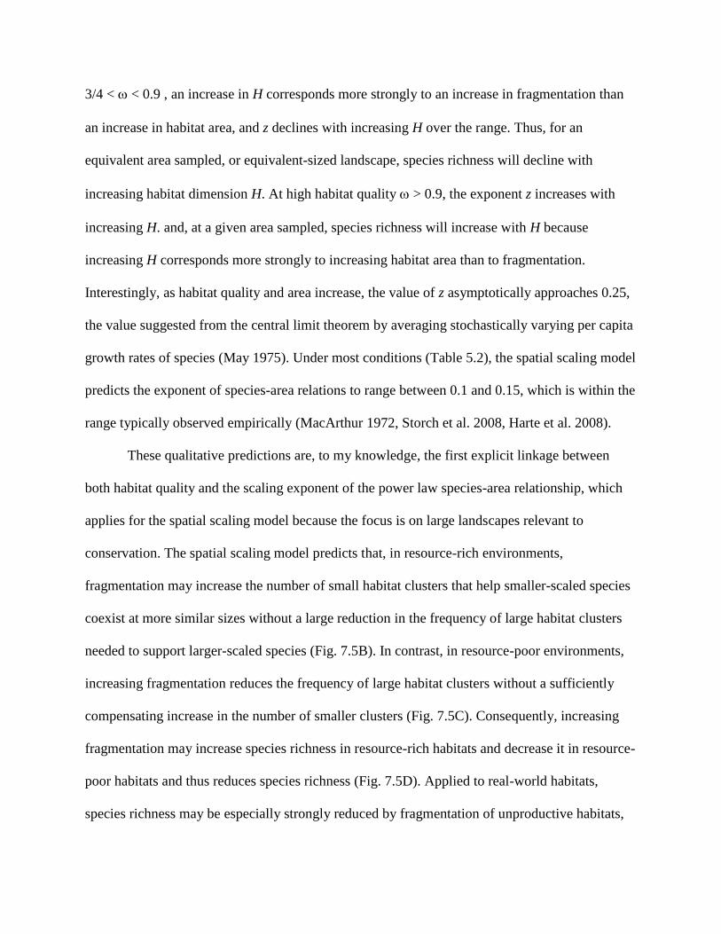
3/4 < < 0.9 , an increase in H corresponds more strongly to an increase in fragmentation than

an increase in habitat area, and z declines with increasing H over the range. Thus, for an

equivalent area sampled, or equivalent-sized landscape, species richness will decline with

increasing habitat dimension H. At high habitat quality > 0.9, the exponent z increases with

increasing H. and, at a given area sampled, species richness will increase with H because

increasing H corresponds more strongly to increasing habitat area than to fragmentation.

Interestingly, as habitat quality and area increase, the value of z asymptotically approaches 0.25,

the value suggested from the central limit theorem by averaging stochastically varying per capita

growth rates of species (May 1975). Under most conditions (Table 5.2), the spatial scaling model

predicts the exponent of species-area relations to range between 0.1 and 0.15, which is within the

range typically observed empirically (MacArthur 1972, Storch et al. 2008, Harte et al. 2008).

These qualitative predictions are, to my knowledge, the first explicit linkage between

both habitat quality and the scaling exponent of the power law species-area relationship, which

applies for the spatial scaling model because the focus is on large landscapes relevant to

conservation. The spatial scaling model predicts that, in resource-rich environments,

fragmentation may increase the number of small habitat clusters that help smaller-scaled species

coexist at more similar sizes without a large reduction in the frequency of large habitat clusters

needed to support larger-scaled species (Fig. 7.5B). In contrast, in resource-poor environments,

increasing fragmentation reduces the frequency of large habitat clusters without a sufficiently

compensating increase in the number of smaller clusters (Fig. 7.5C). Consequently, increasing

fragmentation may increase species richness in resource-rich habitats and decrease it in resource-

poor habitats and thus reduces species richness (Fig. 7.5D). Applied to real-world habitats,

species richness may be especially strongly reduced by fragmentation of unproductive habitats,

such as deserts, oligotrophic lakes, polar tundra, etc., while species richness may be enhanced by

moderate fragmentation in more productive habitats like tropical rainforests, eutrophic lakes and

wetlands (Chase and Leibold 2003).

These results lead to further qualitative predictions about how species richness should

increase with habitat area. Species richness should increase more rapidly with habitat area or

proportion, h, in fragmented habitats, with higher H, than in aggregated habitats (Fig. 7.6). At

low h, what habitat remains is aggregated into sufficiently large clusters to sustain larger-scaled

species, and thus, for a given area of habitat, a lower H will sustain more species. In contrast, at

high h, smaller-scaled species can coexist at more similar sizes because there is a much higher

frequency of smaller habitat clusters but sufficient large clusters to support larger-scaled species.

If habitat quality is high enough, species richness may be higher in more fragmented habitats.

These qualitative predictions are based on power law species area relations. In many

cases, studies explore species incidence or species richness as function of untransformed habitat

area rather than the logarithm of habitat area (With and King 1995, Fahrig 2002). If the

qualitative predictions in Fig. 7.6A are plotted versus untransformed habitat area, one quickly

detects “threshold” effects in which species richness or incidence declines much more

dramatically below a certain proportion of landscape occupied by habitat (Fig. 7.6B). For the

exponents (z = 0.1 – 0.25) expected for most habitats (Fig. 7.5) and observed in the guilds

examined in Chapter 5 (Table 5.1), this sharp downturn will occur in the range of 0.05 < h <

0.15, or around h = 10%. This is consistent with the results of relatively detailed simulations of

species demography, dispersal, and incidence in response to fragmented habitats (Andrén 1994,

With and Crist 1995, With and King 1999, Fahrig 2001). This threshold of species loss may

occur at a slightly higher h in more fragmented habitats or at a similar threshold of h that is

independent of H. This outcome suggests that the trade-off between supporting larger-scaled

species in rarer but more aggregated habitats and more smaller-scaled species in fragmented but

more abundant habitats induces robustness in the generic rule of thumb, suggested by landscape

fragmentation studies, that perceived catastrophic losses of populations and species should not

occur until a habitat has declined to < 10%. In other words, this 10% rule may hold regardless of

whether a habitat is fragmented or not (Fahrig 2002, Radford et al. 2005).

What may matter a great deal for the conservation of species is whether the loss of habitat

results in a reduction of habitat quality, (Vance et al. 2003) One can imagine that higher

quality or more productive habitats, such as those on richer soils or with greater access to water,

may be preferentially removed, effectively reducing both h and . If so, species incidence and

richness may decline more precipitously with the loss of habitat than predicted by the 10% rule,

and increasing H for a given h may exacerbate the effect. Many fewer studies have documented

effects of habitat loss and fragmentation on habitat quality, probably because quality is much

more difficult to measure across landscapes and with remote sensing techniques. The analysis in

this chapter suggests a renewed urgency for assessing whether habitat loss also induces or is

accompanied by a decline in habitat quality and whether such an effect leads to loss of species at

higher habitat proportions than expected.

In contrast with this somewhat gloomy prognosis, the above results of the spatial scaling

model suggest that habitat aggregation, or lowering H for a given h, may fairly successfully

mitigate species losses under habitat loss (Trzcinski et al. 1999). The relationships in Fig. 7.6

suggest that preserving a few, large habitat areas may preserve a larger fraction species than

expected for a given proportion of habitat, which uses the qualitative predictions of the spatial

scaling model to reconstitute the old SLOSS (Single Large Or Several Small) debate (Diamond

1975, Simberloff 1982, 1984, Kunin 1997, McCarthy et al. 2006) as one of FLOMS (Few Large

or Many Small). In particular, conserving more aggregated habitat may be critical in supporting

the larger-scaled, and thus larger-sized species that are often of greatest charismatic interest. In

contrast, inherently smaller-scaled species such as arthropods may have thresholds of minimum

habitat cluster size that lie far below the scales of resolution at which habitat is mapped for

reserve design, and thus the diversity of these species may be related mostly to proportion of

habitat rather than habitat fragmentation (Olff and Ritchie 2002, Hoyle and Harborne 2005).

This entire analysis obviously oversimplifies the full range of issues in conservation, as

the SLOSS debates and other simplified conservation models have also done in the past. In

particular it assumes that species can readily disperse to habitat clusters, and in this sense fails to

capture the “island biogeographic” (MacArthur and Wilson 1967, Hubbell 2001) aspects of

habitat fragmentation that arise from limited dispersal across inhospitable habitat that lies

between suitable habitat clusters (King and With 2002). Nevertheless, the analysis does point out

many ways that resource limitation and scale-dependent constraints and trade-offs might shape

the patterns of species richness with habitat loss and fragmentation. The spatial scaling model

thus presents several testable alternative hypotheses about how habitat loss and fragmentation

might affect the incidence and richness of species and how different management or reserve

design strategies might aid species conservation. These hypotheses are directly connected to the

distribution of food and resources on landscapes and firmly introduce the concept of habitat

quality into the discussion.

Species Persistence and Diversity on Real Landscapes

It is far beyond the scope of this book to provide a detailed and comprehensive review of studies

of the effects of habitat fragmentation on species conservation. However, I offer a few examples

in which a fractal geometric approach has been employed as a way of illustrating how the

qualitative predictions of the spatial scaling model might be tested. To this end, I explore some

examples from my own work (Olff and Ritchie 2002) plus those from some selected field studies

of patterns in bird communities (Vickery et al. 1994, Radford et al. 2005)

Han Olff and I analyzed the incidence of particular species and species richness of bird

and butterfly (Lepidoptera) communities reported for 36 different landscapes in the Netherlands,

each 9 x 9 km (Olff and Ritchie 2002). The habitat of interest is heathland, a type of native

shrub/grassland on low-nutrient soils highly reduced in landscape cover and fragmented by

centuries of agriculture and urban development in northern Europe. Heathlands support many

species of conservation interest, particularly birds, butterflies and plants. In each of the 36

landscapes, heathland habitat was digitized from 1:50.000 scale topographic maps that

differentiated habitat at 250 m resolution. We calculated fractal dimension of heathland habitat

according to the mass fractal method (Milne 1992) with a much coarser resolution than we used

in our original paper (Fig. 7.1), which yielded a wide range of values of h and H across the

landscapes (Fig. 7.3).

To explore the influence of h and H on species incidence and richness, we used data on

the occurrence of all higher plant species, breeding birds and butterflies collected in 1 x 1 km

grids nested within these landscapes between 1970 and 1990 in annual surveys by volunteers,

with the data collection managed by several Dutch NGOs (SOVON for birds, Vlinderstichting

for butterflies, and FLORON for plants). We used the aggregated data over time for this period,

as not much has changed to the landscape spatial structure over this time period. We explored

patterns for species especially associated with heathlands , since more generalized species that

also used heathlands in addition to other habitats would obviously be unlikely to respond only to

heathland habitat distribution and cover.

Species incidence

To test whether species incidence increased with cover and declined with increasing

fragmentation, we chose as an example the largest bird species, black grouse (Tetrao tetrix).

Using logistic regression, we found that the presence or absence of black grouse across the 36

landscapes increased significantly with total cover of heathlands (Fig. 7.7A) but decreased with

increasing habitat fractal dimension, or fragmentation, given h (Fig. 7.7B), as predicted

qualitatively by the spatial scaling model (Eqn 7.13). Further analysis suggestes that black

grouse occupy landscapes very nearly only with habitat clusters > 1 km2 (Olff and Ritchie 2002),

also as predicted by the spatial scaling model (Eqn. 7.14).

These results for the Dutch heathlands are further supported by an example pair of field

studies. One (Vickery et al. 1994) explored habitat patch sizes > 1 ha that were used by different

specialist grassland bird species associated with coastal dune grasslands spatially isolated by

ocean, marshes and forests in Maine, USA. They found that larger bird species occurred only in

larger grassland patches. My own analysis of their data shows that the minimum patch area in

which each species was found increased with body length, the surrogate for sampling scale I

have used in all previous chapters, according to a power law with an exponent of 3.12 (Fig.

7.8A), which is very close to the lower value (3.2-4) predicted by the spatial scaling model (Eqn

7.14).

In another study (Holland et al. 2005), the radius at which forest cover was measured

affected the sensitivity of longhorn beetle (Coleoptera: Cerambycidae) incidence to forest cover.

Through application of an algorithm that explored sensitivity of beetle incidence vs. the radius of

a circular window at which forest cover is measured, Holland et al. (2005) showed that the radius

at which each of 12 generalist species showed their strongest response to forest cover can be

interpreted as proportional to the length of the smallest forest patch that will be occupied by

beetles of different length. This length scale was significantly correlated with beetle body length,

with an exponent of slightly more than 2 (Fig. 7.8B). Eqn 7.14 relates area sampled by the

observer to organism sampling scale, but can be converted to relating observation area length to

sampling scale by taking the square root of both sides. This then predicts a scaling exponent of

1+H/2, which is likely less than the slope of the ln-ln relationship in Fig. 7.8B. Although these

studies had either small sample sizes (Vickery et al. 1994) or somewhat creative measures of

habitat patch scale (cluster size) (Holland et al. 2005) both datasets suggest a power law

quantitative relationship between habitat cluster size, incidence and consumer sampling scale

predicted by the spatial scaling model.

Species Richness Patterns

For the Dutch heathlands (Olff and Ritchie 2002), breeding heathland specialist bird species

richness increased, as expected, with habitat cover (Fig. 7.9A). After controlling for this effect,

bird species richness declined significantly with increasing H (Fig. 7.9B) This result is consistent

with the spatial scaling model’s qualitative predictions.

In contrast to the results for birds, butterfly species richness in Dutch heathlands increased with

habitat cover, but did not decline significantly with increasing H (Fig. 7.9 C, D). The coarse

resolution of mapping may mean that all mapped heathland habitat clusters were large enough to

support any of the butterfly species. Clusters small enough to not support larger butterflies might

not have been mapped or might have been aggregated with other clusters. Alternatively, habitat

quality to butterflies may be higher than for birds, such that butterfly richness is insensitive to

fragmentation while bird richness declines with fragmentation. Thus the spatial scaling model

leads to a fresh alternative hypothesis that might be tested by comparing bird or insect

demography across habitat clusters in relation to plant species composition or density and then

using vegetation data to independently assess habitat quality.

Many other studies show similar patterns of diversity with habitat area. Typical studies

like these, but with particular relevance to the qualitative predictions of the spatial scaling model,

are recent studies of bird species richness in relation to forest cover. In Australia, Radford et al.

(2005) found that landscapes with aggregated habitat had higher species richness at low habitat

cover (small habitat area) while landscapes with fragmented habitat had higher species richness

at higher habitat cover (large area) (Fig. 7.10). Although the interaction term in the Analysis of

Covariance with habitat area and aggregation as factors was not significant, it was nearly so (P =

0.078). Furthermore, species richness, when plotted vs habitat area on a linear scale, declined

rapidly at habitat cover < 10% for both the aggregated and fragmented landscapes. These two

patterns are predicted by the spatial scaling model and the 10% threshold (With and Crist 1995)

has been found in many other studies (Fahrig 2002).

Similarly, bird species richness increased with habitat area in European landscapes

(Storch et al. 2008) with a species-area relationship of slope z = 0.15 after dividing the exponent

for line transect data, 0.3, by 2 to convert length into area. In addition the species area curve over

virtually the full range of areas sampled matched very closely with that predicted by a pure

fractal distribution of habitat.

These examples and their correspondence to qualitative and quantitative predictions of

the spatial scaling model illustrate the possibilities for connecting consumer-resource theory to

landscape ecology and biodiversity conservation. As was seen in predictions for the structure and

diversity of guilds in local habitats (Chapters 5, 6), the critical components of this connection are

scales of the observer and organism and heterogeneity, in this case in the form of aggregated or

dispersed clusters of habitat. In my view, these examples point to a much richer general,

analytical theory of landscape ecology and a plethora of hypotheses to test with further field

observations and experimental tests.

SUMMARY

1. The explicit formulation of food and resource distributions developed for the spatial

scaling model provides the basis for a model of species incidence and richness in

potentially fragmented habitats. The model thus has implications for the conservation of

species and biodiversity.

2. Habitats that are fractal can exhibit variation in their fractal dimension H for a given

proportional cover of habitat h across a landscape, and increasing H is associated with

greater fragmentation for a given h.

3. Criteria from the spatial scaling model derived from its predictions for maximum

sampling scale (size) as a function of area and for species-area relationships can be used

to derive new predictions for how species incidence and diversity should respond to

increasing habitat area, fragmentation, and quality (resource density). Minimum habitat

cluster size is predicted to scale directly with species’ sampling scale (size) with an

exponent of 3.2 in rare habitats to 4 in abundant habitats.

4. Species-area relations depend on both habitat distribution and quality. Aggregation of

habitat can mitigate habitat loss, especially in poorer quality or less productive habitats.

In contrast, aggregation may lead to lower species richness in more productive habitats.

5. The exponent, z, for power law species-area relationships depends as strongly on habitat

quality as area, but may be relatively insensitive to habitat fragmentation except in the

poorest and richest quality habitats. The exponent is predicted to lie between 0.1 and 0.15

for most habitats, considerably lower than the exponent derived from a lognormal

distribution of abundances (May 1975).

6. Empirical studies of species incidence and richness across landscapes with different

proportions and aggregation of habitat generally support the qualitative predictions of the

spatial scaling model and suggest that it may provide considerable insights and

hypotheses about the effects of landscape management on species extinction and

persistence and biodiversity.

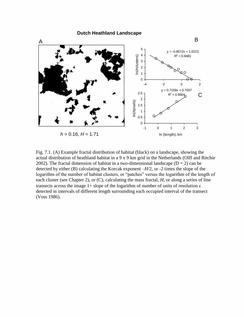
Fig. 7.1. (A) Example fractal distribution of habitat (black) on a landscape, showing the

actual distribution of heathland habitat in a 9 x 9 km grid in the Netherlands (Olff and Ritchie

2002). The fractal dimension of habitat in a two-dimensional landscape (D = 2) can be

detected by either (B) calculating the Korcak exponent –H/2, or -2 times the slope of the

logarithm of the number of habitat clusters, or “patches” versus the logarithm of the length of

each cluster (see Chapter 2), or (C), calculating the mass fractal, H, or along a series of line

transects across the image 1+ slope of the logarithm of number of units of resolution

detected in intervals of different length surrounding each occupied interval of the transect

(Voss 1986).

Dutch Heathland Landscape

h = 0.16, H = 1.71

y = -0.8572x + 1.0223

R2 = 0.9481

0

1

2

3

4

5

-4 -2 0 2

ln (length), km

ln(#

clu

ste

rs)

y = 0.7159x + 0.7007

R2 = 0.9904

0

0.5

1

1.5

2

2.5

-1 0 1 2 3

ln (length), kmln

(#p

ixe

ls)

B

C

A

Fig. 7.2. For two Dutch landscapes with similar proportions (0.16) of heathland habitat but a

aggregated (black circles) vs. fragmented (open circles) degree of aggregation, a plot of the

logarithm of the number of habitat clusters (sets of contiguously occupied units of resolution

along a series of line transects). The slopes of the lines are expected to be –H/2, where H is

the habitat fractal dimension, and thus -0.71 for the fragmented and -0.645 for the aggregated

landscape . The slope of the line for the fragmented habitat is significantly steeper (P < 0.01)

than that for the aggregated habitat. Not also that the frequency of large habitat patches (> 1

km) is much higher for the aggregated landscape.

Fig. 7.3. Example 9 x 9 km fractal landscapes in the Netherlands selected to illustrate the

relationship between fractal dimension H of heathland habitat (black) and proportion of

landscape occupied by habitat h. H increases with h (bottom row to top row) but also with the

degree of habitat aggregation (right to left). Thus for a given amount of habitat, h, a lower fractal

dimension H indicates a greater degree of fragmentation of the habitat into smaller clusters.

Fig. 7.4 Relationship between fragmentation index (number of habitat clusters or

patches/habitat area) and the habitat fractal dimension H, independent of h, the proportion of

landscape occupied by the habitat. H is the habitat fractal dimension at which fragmentation is

minimized or aggregation is maximized for a given landscape extent, x.

Fig. 7.5. A. Hypothetical exponent z of the approximate species-area relationship for large

landscapes S Az over a conservation-relevant range of habitat fractal dimensions (2 > H > H >

1.2) for high quality (resource-dense) and low quality (resource-scarce) habitats. B., C. Shift in

the power law frequency distributions of habitat cluster sizes resulting from an increase in H for

B. high quality and C. low quality habitats. D. Resulting species-area curves implied by A-C for

high and low quality habitats.

Fig. 7.6. Hypothetical influence of habitat area and fragmentation on species richness of a guild,

plotted in (A) logarithmic space and (B) linear space. Graphs show the greater sensitivity of

fragmented habitats to reduction in habitat area but the quicker saturation of species richness

with increasing area in aggregated habitats.

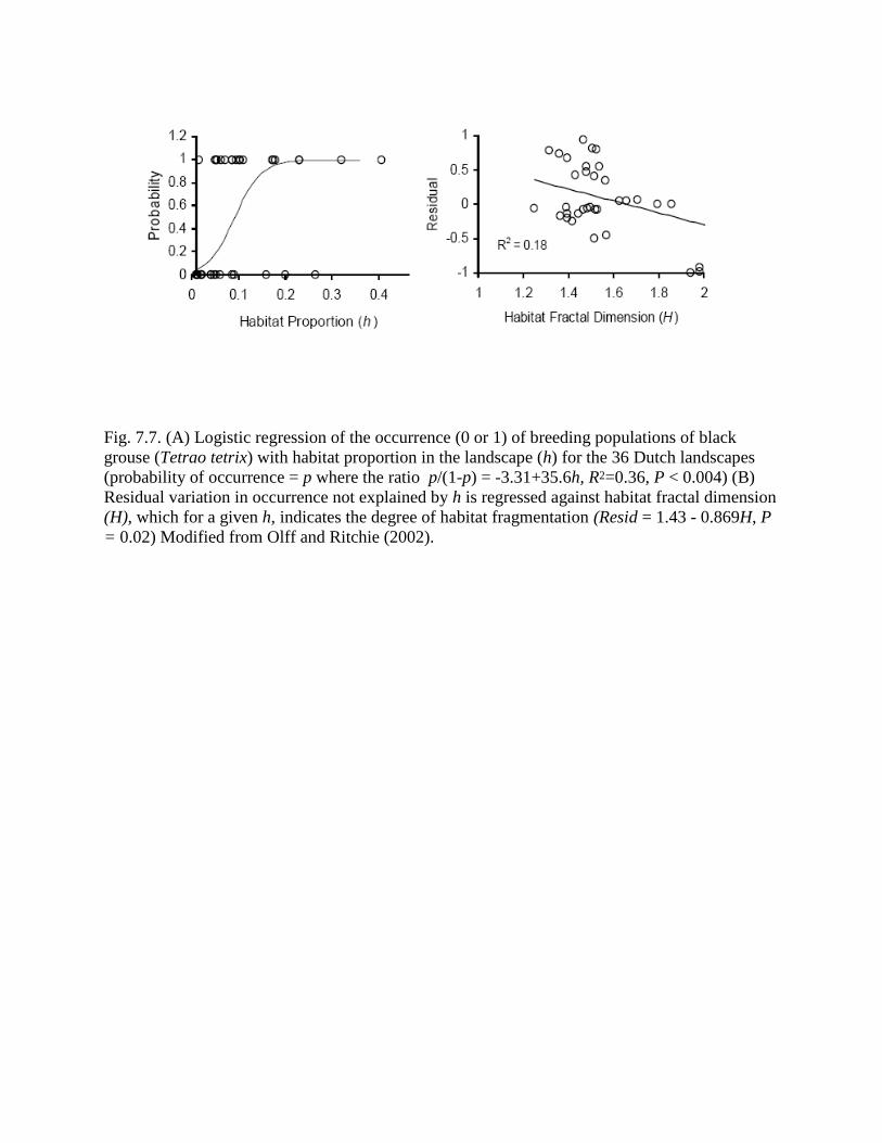
Fig. 7.7. (A) Logistic regression of the occurrence (0 or 1) of breeding populations of black

grouse (Tetrao tetrix) with habitat proportion in the landscape (h) for the 36 Dutch landscapes

(probability of occurrence = p where the ratio p/(1-p) = -3.31+35.6h, R2=0.36, P < 0.004) (B)

Residual variation in occurrence not explained by h is regressed against habitat fractal dimension

(H), which for a given h, indicates the degree of habitat fragmentation (Resid = 1.43 - 0.869H, P

= 0.02) Modified from Olff and Ritchie (2002).

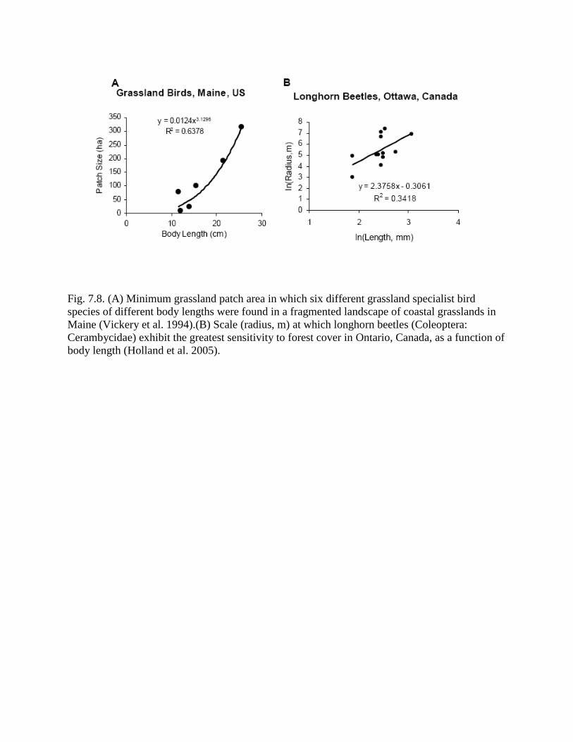
Fig. 7.8. (A) Minimum grassland patch area in which six different grassland specialist bird

species of different body lengths were found in a fragmented landscape of coastal grasslands in

Maine (Vickery et al. 1994).(B) Scale (radius, m) at which longhorn beetles (Coleoptera:

Cerambycidae) exhibit the greatest sensitivity to forest cover in Ontario, Canada, as a function of

body length (Holland et al. 2005).

Fig. 7.9. Regressions of heathland bird species richness A,B and butterfly species richness (C, D)

with proportion (h) of heathland habitat across 36 Dutch landscapes (9 x 9 km areas, see Fig.

7.3). B, D) Residual variation not explained by h is regressed against fractal dimension (H). Note

that residual bird species richness, after accounting for the effects of habitat amount in A),

declines significantly with increasing H, which for a given h indicates the degree of habitat

fragmentation. Not also that this pattern for butterflies was not significant (P > 0.05). Modified

from Olff and Ritchie (2002).

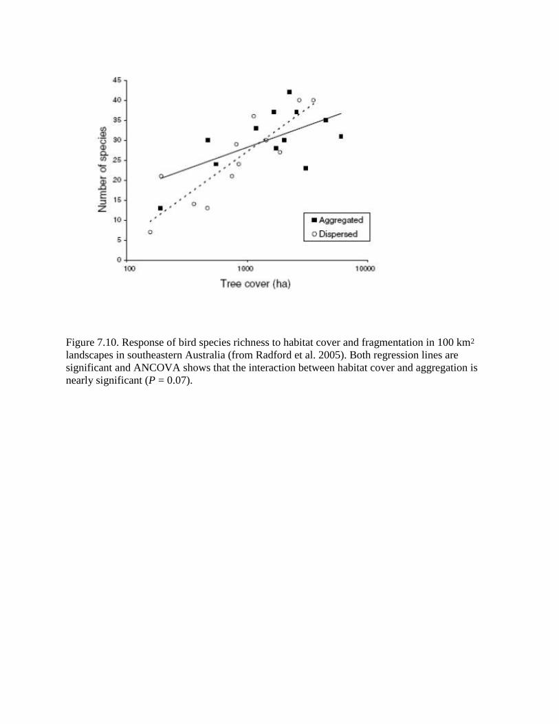
Figure 7.10. Response of bird species richness to habitat cover and fragmentation in 100 km2

landscapes in southeastern Australia (from Radford et al. 2005). Both regression lines are

significant and ANCOVA shows that the interaction between habitat cover and aggregation is

nearly significant (P = 0.07).