3-17-05 Che505_bio.doc

CHAPTER 14 ChE 505: Biochemical Reaction Engineering Application Examples Biochemical reactions are encountered in a number of environmentally important processes. Some examples are shown here

1. Secondary treatment of wastewater Wastewater undergoes first a primary treatment. Here the suspended solids are

removed. The wastewater now has colloidal matter and dissolved organic compounds. They are then treated by feeding them to microorganisms which use the dissolved organics as their food and converts the waste to CO2 and H20. The organism grow and multiply thus converting the dissolved organic to a solid waste (sludge) which can be settled and removed. The water is thus purified. Activated sludge process is a common example. Here the treatment takes place in open tanks with either surface aeration or submerged aeration to provide enough oxygen for the microorganisms. There are many other processes to do this as well, for example, the trickling filter. Nutrients such as N and P are needed for the growth of biomass and these are usually present in the wastewater. In some cases there is excess of nutrient and removal of these may be necessary (see #2 below). In other cases an external supply of nutrient has to be provided.

2. Biological nutrient removal. In some cases there is excess of nutrient in wastewater and only a part of these may

be utilized for biomass growth. The excess nutrient in discharged water has many negative environmental consequences. e.g eutrophication, (excess of nutrients leading to algae growth etc) oxygen depletion leading to fish kill etc. hence. removal of these nutrients may be necessary by additional step or as a simultaneous step during the removal of dissolved organics. The process is known as BNR (biological nutrient removal).

3. Anaerobic treatment of wastewater Under suitable conditions, wastewater can also be treated under anaerobic conditions.

In contrast, to aerobic process, the anaerobic process is an energy producing process since the byproduct is methane. The quantity of sludge produced is also smaller. Since the sludge disposal costs are often 50% of the wastewater treatment costs this represents a saving as well. Nutrient loadings are also smaller.

The treated effluent has however, a higher concentration of dissolved organic. This can be problematic and some form of post-treatment (usually a aerobic treatment) may be needed before the water can be discharged to surfaces. Thus the process is more suitable for relatively high concentration waste streams. (more than 4kg of COD per cubic meter of water).

4. Soil bioremediation Soil remediation is the removal of contaminants from soil either by convective transport techniques, such as flushing, soil vapor extraction and sparging, and by biological degradation. Bioremediation uses naturally occurring microorganisms to degrade wastes in the soil at the polluted site. Moisture and pH of the soil, availability of oxygen to the microorganisms, temperature and nutrients are important factors in treatment effectiveness. Alkanes, benzene and tetrachloroethene are examples of chemicals that can be degraded by bioremediation. COD and Yield Coefficient COD is a lumped concept useful to characterize waste water. kg /m3 is the common unit. For a solution of known composition COD can be calculated by a simple stoichiometry of combustion reaction. Organic compounds usually fit a general formula of CαHβOγNδ and the combustion reaction can be represented as

2222 224NOOHCOONOHC δβαδγβαδγβα ++→⎟

⎠⎞

⎜⎝⎛ +−++

The substrate kinetics is established by noting that as the organisms grow, the substrate is utilized. Thus the rate of substrate consumption is directly related to the microbial growth rate by a proportionality constant.

dtdSY

dtdS

UdtdX

−=−=1

Here U is called the specific substrate utilization rate. It is also the reciprocal of Y, the specific yield of organisms. Both U and Y are like stoichiometric factors familiar in reaction engineering. In many cases these can be predicted by setting up a reaction stoichiometry. A general molar representation of biomass is C5H7NO2. Some examples are shown below: Yield calculations: Example 1: Oxygen requirements and Y factor: Use of reaction stoichiometry to compute Y and COD is illustrated below. Reaction is represented by an overall stoichiometry

OHvCOvcellsnewvPOvNHvOvorganicv ismmicroorgan27265

34433221 )()( ++⎯⎯⎯⎯ →⎯+++ −

Based on this Y and O2 demand can be calculated. Assume organic is glucose and the biomass has a structure C5H7NO2. A balanced reaction is then

OHCONOHCNHOOHC 22275326126 1482283 ++→++ 3(180) 8(32) 2(17) 2(113)

Biomass produced = 226 g O2 consumed = 256 g Glucose consumed = 540 g O2 demand = 256/540 = 0.47 g / g glucose Y per glucose = 226/540 = 0.42 g cells / glucose Also U = 1/0.42 = 2.38 g glucose consumed to produce 1 g of cell. It is more convenient to write this in terms of COD (chemical oxygen demand). For this purpose COD of glucose is calculated as follows: COD of glucose:

OHCOOOHC 2226126 666 +→+ 180 192

COD = 192/180 = 1.07 g O2/g glucose Y = 0.42 g cells / g glucose x g glucose / 1.07 COD = 0.392 g cells / g COD A second approach is to write half reactions for the various oxidation and reduction processes and balance the rate of these processes. This method is described below. Consider again the substrate to be glucose. Oxidation is the electron donor half reaction, shown by equation (2), with rate Rd.

−+ ++→+ eHCOOHOHC 226126 41

41

241 (2)

Reduction is the electron acceptor half reaction that has two possible routes; respiration, equation (3a), and synthesis, equation ( 3b) that proceed at the rate Rc, and Rs , respectively:

A. Respiration

OHeHO 22 21

41

→++ −+ (3a)

B. Synthesis (in presence of nitrates)

OHNOHCeHCONO 227523 2811

281

2819

225

281

+→+++ −+− (3b)

In the above we have assumed that organic matter (food) is the simple sugar (glucose) and that the culture in question can utilize the nitrate ion to synthesize new biomass by equation (3b). Now, based on data, we assume that the probability of reaction (3a) occurring is fe while the probability of reaction (3b) occurring is fs. Clearly, since the electron must be used by ether route (3a) or (3b), we must have fe+fs=1. In addition, the rate of electron production must equal the rate of electron consumption so that

Rd + fs Rs + feRc = 0 (4) Now, if based on available information we conclude that fs=0.68, and hence fe=1-0.68=0.28, then substituting these values in equation (4) leads to the overall stoichiometry below. Overall stoichiometry

OHCONOHCHONOOHC 22275236126 184.014.00221.00221.0095.00221.0241

++→+++ +−

(5) Now, if we know the O2 uptake rate we can determine the nitrate or glucose consumption rate and rate of synthesis of cell mass! Unfortunately, in most real complex systems we do not know that and we need to rely on empirical yield factors defined earlier. . The factors, fe and fs can also be related to the free energy changes associated with the respiration and synthesis reaction. The free energy determines how the released energy is partitioned into respiration vs synthesis. The suggested relation for heterotropic bacteria is

R

s

e

e

s

e

GkG

ff

ff

∆∆

−=−

=1

sG∆ = energy required for cell synthesis which is calculated by Eq (1) shown later.

k = fraction of energy captured

RG∆ = energy released from the oxidation-reduction reactions (from the overall process of oxidation and respiration) The value of is free energy to convert 1-electron equivalent of carbon source to cell material. This is estimated as

sG∆

kG

GkmG

G Nc

ps

∆+∆+

∆=∆

pG∆ = free energy to convert 1- electron equivalent of carbon source to pyruvate

intermediate. m = +1 if is positive or –1 if energy is produced. pG∆

cG∆ = free energy to convert 1- electron equivalent of pyruvate to 1- electron equivalent of cells. This is normally taken as +31.41 kJ/e-eq

NG∆ = free energy per 1- electron equivalent of cells to reduce nitrogen to ammonia. This factor accounts for the fact that a nitrogen source has to be converted to ammonia if N2 is not available in the form of ammonia. The values of 17.46, 13.6, 15.81 and 0.0 are used for , , N−

3NO −2NO 2 and respectively. Tables of ∆G values are available for a

number of typical bio-chemical half reactions. The values for some reactions are attached here. An illustrative problem is solved below.

+4NH

Example: Consider acetate as a substrate and CO2 as the electron acceptor. This represents the treatment under anaerobic condition in the absence of oxygen. Find fe and fs based on free energy considerations. Take the fraction of energy used as 0.6 Solution The oxidation half reaction is represented as

−+−− +++→+ eHHCOCOOHCOOCH 3223 81

81

83

81

and has a free energy of –27.68 kJ per electron from the tabulated values. In the absence of O2 (anaerobic conditions) the CO2 acts as an electron acceptor. The respiration reaction is then represented as

OHCHeHCO 242 41

81

81

+→++ −+

and the free energy is 24.11 kJ/g. eq. of electrons Overall free energy change is therefore –27.68+24.11 = -3.57 kJ which is our ∆GR value. The free energy of pyruvate formation is now calculated. This is reaction 15 in the table.

OHCOCOOCHeHHCOCO 2332 52

101

101

51

+→+++ −−+−

∆G = 35.78 kJ. Note that the overall pyruvate formation is the sum of oxidation half reaction and the above pyruvate half reaction. Hence ∆Gp = -27.68 + 35.78 = 8.1 kJ which is positive. Energy is utilized in pyruvate formation for this substrate (acetate) and m is taken as 1. Note in a general context that puruvate formation from other substrates such as glucose releases energy and is the first step in the Kreb cycle by which we (all species) use the food energy. Assume k = 0.6.

∆Gs = 8.1 / 0.6 + 31.41 + 0 = 44.91 kJ/mole.

96.20)57.3.(6.0

91.441

=−

−=

− e

e

ff

solving gives fe = 0.9547 and fs = 0.046 g cell / g COD used. Tables:

Kinetics of Microbial Reactions The growth of the microbial concentration follows a first order dependence and can be described as:

Rx = XdtdX µ=

where X is the concentration of the micro-organisms and µ is a growth constant and Rx is the rate of growth (kinetic model) for biomass. An early model by Monod (1942) showed that the growth constant is a function of the nutrient or the substrate concentration. The relation can be described by the following equation.

SKS

s += maxµµ

where S is the concentration of the substrate and µmax is a maximum growth constant. The other constant in the model is Ks. In fact, it can be shown that if S = Ks /2 the growth rate is half the maximum value. Hence Ks is also called the half velocity constant. The Monod’s equation applies to pure cultures but is also applied to mixed cultures as a first approximation. Other models for the growth constant µ have also been proposed. Thus Haldane proposed the following model

Is K

SSK

S2max

++= µµ

where KI is often referred to as the substrate inhibition constant. In a dynamic growth situation, some organisms are born, some die and some members simply grow in mass. The death rate is added to the model by adding a decay constant and the net growth rate of microbes is represented as:

XkXSK

SXkXR ds

dx −+

=−= maxµµ

Although the model is simple (a lumped model for microbes), it has served its purpose well in many applications. However, more complete models that incorporate some of the

underlying biochemical mechanisms offer a better representation and predictability. Such models are based on metabolic pathway analysis. Such detailed models are often developed if there are certain design objectives in mind. Otherwise a simple Monod based model is often sufficient. Typical values of kinetic parameters for domestic wastewater at 20degC are in the following range: µmax 2-10 g bsCOD/g VSS. Day Ks. 10-60 mg/L bsCOD Y 0.3-0.6 mg VSs/mg bsCOD Kd 0.06-0.15 gVSS/ g VSS day Here bsCOD refers to biodegradable soluble chemical oxygen demand. VSS refers to volatile suspended solids which is commonly used as a measure of biomass concentration since this is an easily measurable quantity, Materials that can be volatilized and burned off when ignited at 500 +or- 49 deg C are classified as volatile The effect of temperature on the kinetic parameters is of some interest. The growth constant µmax increases with temperature and reaches a maximum and then decreases rapidly with temperature. This is often fitted by two Arrhenius type of parameters: The Monod constant is an inverse function of temperature and is fitted as:

⎟⎠⎞

⎜⎝⎛ −=

RTEA

K s

1exp1

The yield constant is assumed to be independent of temperature. Other effects such as product poisoning may have to be added to the model. One example is alcohol production by fermentation where higher concentrations of alcohol act as poison to the microbial population. Detailed kinetic models In this model one attempts to track the key species involved in the process rather than lumping all the species into COD.

Metabolic Pathway Models As an example of metabolic pathway analysis, the growth metabolism model for E. coli was developed by Schuler and co-workers. This model shown schematically in Fig. 2 has 23 stoichiometric constants and 49 kinetic parameters. Most of the kinetic parameters could be estimated from the large number of reported previous studies on the system. Process Model for Activated Sludge Process The typical flow diagram can be represented as follows: Primary effluent Effluent Q0-Qw, Xe, S Q0, S0, X0 Q0+ QR secondary V,X,S X,S clarifier reactor QR, sludge return sludge Xu Qu,Xu underflow Sludge Qw, Xu waste Control volume/mass boundary (a)

Primary effluent Effluent Q0-Qw, Xe, S Q0, S0, X0 Reactor Q+ QR secondary Variable X,S clarifier X, S QR, sludge return sludge Xu Qu,Xu underflow Sludge waste Qw, Xu Control volume/mass boundary (b) Figure: Schematics of the two general types of activated sludge systems: (a) completely mixed; (b) plug flow Model is developed by writing mass balances for the substrate and the biomass. The model equations for a backmixed reactor are as follows: Cell Balance: Produced – Died = -In + Out

( )[ ]uwewds

XQXQQXQXVkXVSK

S+−+−=−

+ 000maxµ (7.16)

which can be rearranged as

( )d

ewuw

s

kVX

XQXQQXQSK

S+

−−+=

+000

maxµ (7.17)

The same mathematical operations may be applied to the substrate. These will not be repeated but the result will be written at once, which is

( ) XVSKY

S

s +maxµ

= ( )( ){ SQSQQSQ ww }+−+− 000 (7.18)

Eq. (7.18) may be manipulated to produce

( SSVX

YQSK

S

s

−=+ 0

0maxµ ) (7.19)

Equating the right hand sides of Eqns (7-17) and (7-19) and rearranging gives us

( ) ( ) dewuw kSS

VXYQ

VXXQXQQXQ

−−=−−+

00000 (7.20)

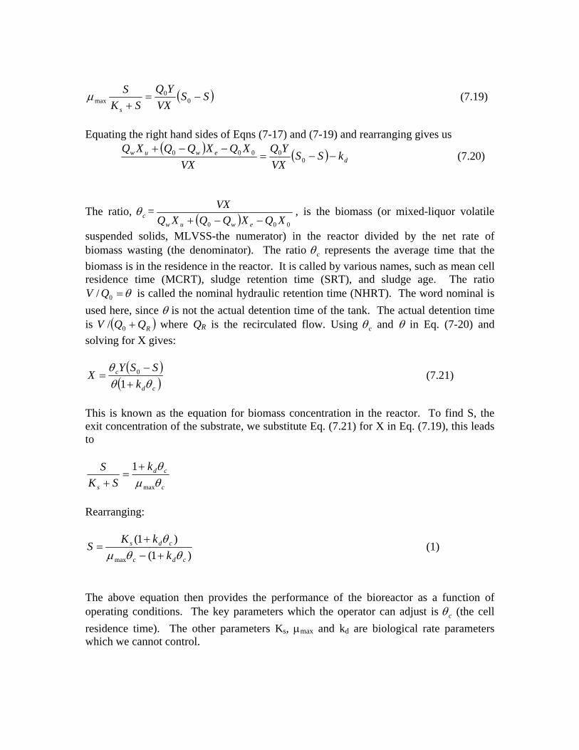
The ratio, cθ = ( ) 000 XQXQQXQVX

ewuw −−+, is the biomass (or mixed-liquor volatile

suspended solids, MLVSS-the numerator) in the reactor divided by the net rate of biomass wasting (the denominator). The ratio cθ represents the average time that the biomass is in the residence in the reactor. It is called by various names, such as mean cell residence time (MCRT), sludge retention time (SRT), and sludge age. The ratio

θ=0/ QV is called the nominal hydraulic retention time (NHRT). The word nominal is used here, since θ is not the actual detention time of the tank. The actual detention time is where Q( )RQQV +0/ R is the recirculated flow. Using cθ and θ in Eq. (7-20) and solving for X gives:

( )( )cd

c

kSSY

Xθθ

θ+

−=

10 (7.21)

This is known as the equation for biomass concentration in the reactor. To find S, the exit concentration of the substrate, we substitute Eq. (7.21) for X in Eq. (7.19), this leads to

c

cd

s

kSK

Sθµθ

max

1+=

+

Rearranging:

)1()1(

max cdc

cds

kkK

Sθθµ

θ+−

+= (1)

The above equation then provides the performance of the bioreactor as a function of operating conditions. The key parameters which the operator can adjust is cθ (the cell residence time). The other parameters Ks, µmax and kd are biological rate parameters which we cannot control.

An interesting effect is that the exit concentration in the bioreactor is independent of the inlet concentration. This is unlike a conventional chemical reactor.

cθ is sometimes referred to as BSRT or biomass solid retention time. The reactor performance depends on cθ (See Eq. 7.21). The concentration of cells in the bioreactor however depends on both cθ and θ. A minimum residence time is required and this is related to the inlet substrate concentration. This quantity can be obtained by setting X = 0 in Eq (7.21). This would be yield at S = S0. Now, using Eq(1) for S and solving, one obtains

⎟⎟⎠

⎞⎜⎜⎝

⎛+>

0max

11SKs

c µθ assuming kd = 0 here.

min,cθ

or 0max

0min, S

SKsc µ

θ+

=

Eq. (1) holds only if the above condition is satisfied. A plot of S vs cθ is as follows: S S0 cθ minimum Cell concentration profiles are as follows: X Low θ case High θ case min cθ

Another important parameter in the design and operation of an activated sludge plant is the recirculation ratio, . R may be obtained by performing a material balance around the secondary clarifier. Since the clarifier is not aerated, dX/dt = 0. Also at

steady state

0/ QQR R=

0=∂∂

tX . Adopting these facts and performing the material balance produces

( ) ( ) ( uwReRR XQQXQQXQQ )++−=+ 00 (7.24) Solving for the ratio gives:

( ) (( )

)XXQ

XXQXXQR

QQ

u

euweR

−−−−

==0

0

0

(7.25)

Trickling Bed System: A schematic diagram is shown in the next page. Often a first order kinetic model is used for simplicity.

a

s

QAk

SS '

ln0

=

k’ = rate constant = k Xf Xf = microbial concentration in the film As = surface area for diffusion into biomass Qa = volumetric flow rate Other detailed models based on Monod’s kinetics can also be derived.