binary phase diagrams -...

MSE 305, Phase Diagrams and Kinetics, Leonid Zhigilei, Fall 2004

Binary phase diagrams

Binary phase diagrams and Gibbs free energy curvesBinary solutions with unlimited solubilityRelative proportion of phases (tie lines and the lever principle) Development of microstructure in isomorphous alloysBinary eutectic systems (limited solid solubility)Solid state reactions (eutectoid, peritectoid reactions) Binary systems with intermediate phases/compoundsThe iron-carbon system (steel and cast iron)Gibbs phase ruleTemperature dependence of solubilityThree-component (ternary) phase diagrams

Reading: Chapters 1.5.1 – 1.5.7 of Porter and Easterling, Chapter 10 of Gaskell


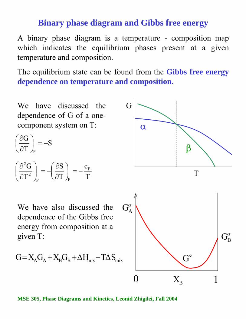
Binary phase diagram and Gibbs free energy

BX 10

αAG

A binary phase diagram is a temperature - composition map which indicates the equilibrium phases present at a given temperature and composition.

The equilibrium state can be found from the Gibbs free energy dependence on temperature and composition.

αBG

αG

We have also discussed the dependence of the Gibbs free energy from composition at a given T:

We have discussed the dependence of G of a one-component system on T:

G

T

β

α

STG

P

−=⎟⎠⎞

⎜⎝⎛

∂∂

Tc

TS

TG P

PP2

2

−=⎟⎠⎞

⎜⎝⎛

∂∂

−=⎟⎟⎠

⎞⎜⎜⎝

⎛∂∂

mixmixBBAA S T∆∆HGXGXG −++=


Binary solutions with unlimited solubility

BX 10

liquidAG

Let’s construct a binary phase diagram for the simplest case: A and B components are mutually soluble in any amounts in both solid (isomorphous system) and liquid phases, and form ideal solutions.

We have 2 phases – liquid and solid. Let’s consider Gibbs free energy curves for the two phases at different T

liquidBG

solidG

T1 is above the equilibrium melting temperatures of both pure components: T1 > Tm(A) > Tm(B) → the liquid phase will be the stable phase for any composition.

liquidG

1T

[ ]BBAABBAAid lnXXlnXXRTGXGXG +++=

solidBG

solidAG


Binary solutions with unlimited solubility (II)

BX 10

solidBG

Decreasing the temperature below T1 will have two effects:

will increase more rapidly than

liquidBG

solidG

Eventually we will reach T2 – melting point of pure component A, where

liquidG

2T

liquidB

liquidA G and G solid

AGsolidBG and Why?

The curvature of the G(XB) curves will decrease. Why?

solidA

liquidA G G =

solidA

liquidA G G =


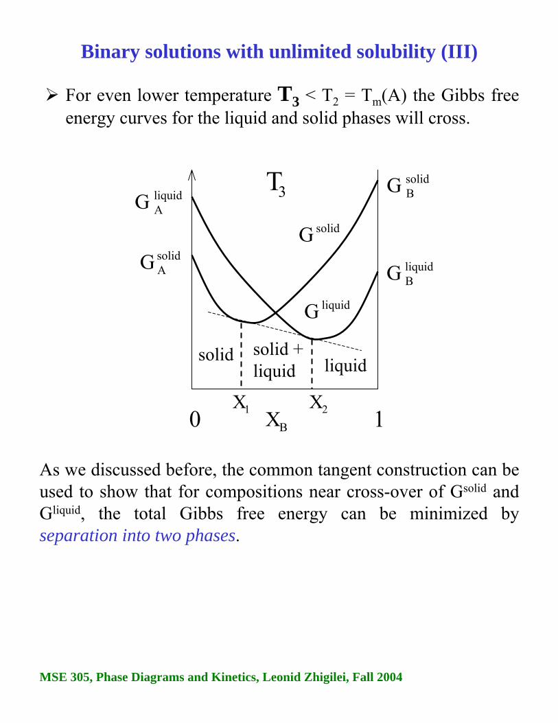
Binary solutions with unlimited solubility (III)

solidBG

For even lower temperature T3 < T2 = Tm(A) the Gibbs free energy curves for the liquid and solid phases will cross.

liquidBG

solidG

liquidG

3T

solidAG

As we discussed before, the common tangent construction can be used to show that for compositions near cross-over of Gsolid and Gliquid, the total Gibbs free energy can be minimized by separation into two phases.

BX 10

solid liquidsolid +liquid

1X 2X

liquidAG


Binary solutions with unlimited solubility (IV)

liquidAG

solidB

liquidB GG =

solidG

liquidG

4T

solidAG

At T4 and below this temperature the Gibbs free energy of the solid phase is lower than the G of the liquid phase in the wholerange of compositions – the solid phase is the only stable phase.

BX 10

As temperature decreases below T3 continue

to increase more rapidly than

Therefore, the intersection of the Gibbs free energy curves, as well as points X1 and X2 are shifting to the right, until, at T4= Tm(B) the curves will intersect at X1 = X2 = 1

liquidB

liquidA G and G

solidB

solidA G and G


Binary solutions with unlimited solubility (V)

solidBG

Based on the Gibbs free energy curves we can now construct a phase diagram for a binary isomorphous systems

liquidBG

solidG

liquidG

3TsolidAG

BX 10

solid liquidsolid +liquid

liquidAG

2T

3T

4T

5T

1TT

4T

2T

1T


Liquidus line separates liquid from liquid + solidSolidus line separates solid from liquid + solid

Binary solutions with unlimited solubility (VI)Example of isomorphous system: Cu-Ni (the complete solubility occurs because both Cu and Ni have the same crystal structure, FCC, similar radii, electronegativity and valence).

Liquid

α

Solid solution

Solidus lineLiquidus line


In one-component system melting occurs at a well-defined melting temperature.

In multi-component systems melting occurs over the range of temperatures, between the solidus and liquidus lines. Solid andliquid phases are in equilibrium in this temperature range.

α + L

α

L liquid solution

liquid solution +

crystallites ofsolid solution

polycrystalsolid solution

Binary solutions with unlimited solubility (VII)

Liquidus

Solidus

A B20 40 60 80Composition, wt %

Tem

pera

ture


Interpretation of Phase Diagrams

For a given temperature and composition we can use phase diagram to determine:

1) The phases that are present

2) Compositions of the phases

3) The relative fractions of the phases

Finding the composition in a two phase region:

1. Locate composition and temperature in diagram

2. In two phase region draw the tie line or isotherm

3. Note intersection with phase boundaries. Read compositions at the intersections.

The liquid and solid phases have these compositions.

BX solidBXliquid

BX


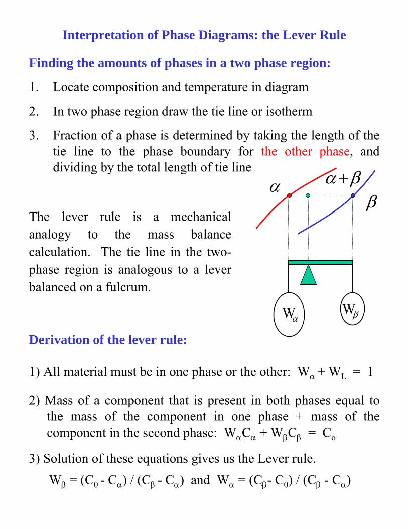
Finding the amounts of phases in a two phase region:

1. Locate composition and temperature in diagram

2. In two phase region draw the tie line or isotherm

3. Fraction of a phase is determined by taking the length of the tie line to the phase boundary for the other phase, and dividing by the total length of tie line

The lever rule is a mechanical analogy to the mass balance calculation. The tie line in the two-phase region is analogous to a lever balanced on a fulcrum.

Interpretation of Phase Diagrams: the Lever Rule

1) All material must be in one phase or the other: Wα + WL = 1

2) Mass of a component that is present in both phases equal to the mass of the component in one phase + mass of the component in the second phase: WαCα + WβCβ = Co

3) Solution of these equations gives us the Lever rule. Wβ = (C0 - Cα) / (Cβ - Cα) and Wα = (Cβ - C0) / (Cβ - Cα)

Derivation of the lever rule:

αW

α βα +β

βW


Composition/Concentration: weight fraction vs. molar fraction

Composition can be expressed in

Molar fraction, XB, or atom percent (at %) that is useful when trying to understand the material at the atomic level. Atom percent (at %) is a number of moles (atoms) of a particular element relative to the total number of moles (atoms) in alloy. For two-component system, concentration of element B in at. % is

Where nmA and nm

B are numbers of moles of elements A and B in the system.

Weight percent (C, wt %) that is useful when making the solution. Weight percent is the weight of a particular component relative to the total alloy weight. For two-component system, concentration of element B in wt. % is

100mm

mCAB

Bwt ×+

=

100nn

nC Am

Bm

Bmat ×

+=

where mA and mB are the weights of the components in the system.

100XC Bat ×=

B

BBm A

mn = where AA and AB are atomic weights of elements A and B.A

AAm A

mn =


Composition Conversions

Weight % to Atomic %:

Atomic % to Weight %:

100ACAC

ACCB

wtAA

wtB

AwtBat

B ×+

=

100ACAC

ACCB

wtAA

wtB

BwtAat

A ×+

=

WL = (Cwtα - Cwt

o) / (Cwtα - Cwt

L)

Of course the lever rule can be formulated for any specification of composition:

ML = (XBα - XB

0)/(XBα - XB

L) = (Catα - Cat

o) / (Catα - Cat

L)

Mα = (XB0 - XB

L)/(XBα - XB

L) = (Cat0 - Cat

L) / (Catα - Cat

L)

Wα = (Cwto - Cwt

L) / (Cwtα - Cwt

L)

100ACAC

ACCA

atAB

atB

BatBwt

B ×+

=

100ACAC

ACCA

atAB

atB

AatAwt

A ×+

=


Phase compositions and amounts. An example.

Mass fractions: WL = S / (R+S) = (Cα - Co) / (Cα - CL) = 0.68

Wα = R / (R+S) = (Co - CL) / (Cα - CL) = 0.32

Co = 35 wt. %, CL = 31.5 wt. %, Cα = 42.5 wt. %


Development of microstructure in isomorphous alloysEquilibrium (very slow) cooling


Development of microstructure in isomorphous alloysEquilibrium (very slow) cooling

Solidification in the solid + liquid phase occurs gradually upon cooling from the liquidus line.

The composition of the solid and the liquid change gradually during cooling (as can be determined by the tie-line method.)

Nuclei of the solid phase form and they grow to consume all the liquid at the solidus line.


Development of microstructure in isomorphous alloysNon-equilibrium cooling


Development of microstructure in isomorphous alloysNon-equilibrium cooling

• Compositional changes require diffusion in solid and liquid phases

• Diffusion in the solid state is very slow. ⇒ The new layers that solidify on top of the existing grains have the equilibriumcomposition at that temperature but once they are solid their composition does not change. ⇒ Formation of layered (cored) grains and the invalidity of the tie-line method to determine the composition of the solid phase.

• The tie-line method still works for the liquid phase, where diffusion is fast. Average Ni content of solid grains is higher. ⇒ Application of the lever rule gives us a greater proportion of liquid phase as compared to the one for equilibrium cooling at the same T. ⇒ Solidus line is shifted to the right (higher Ni contents), solidification is complete at lower T, theouter part of the grains are richer in the low-melting component (Cu).

• Upon heating grain boundaries will melt first. This can lead to premature mechanical failure.


Binary solutions with a miscibility gapLet’s consider a system in which the liquid phase is approximately ideal, but for the solid phase we have ∆Hmix > 0

solidG

liquidG

1T

BX 10

solidG

liquidG12 TT <

BX 10

solidG

liquidG23 TT <

BX 10

T

BX 103T

1T

2T

G

GG

liquid

α

α1+α2

At low temperatures, there is a region where the solid solution is most stable as a mixture of two phases α1 and α2 with compositions X1 and X2. This region is called a miscibility gap.


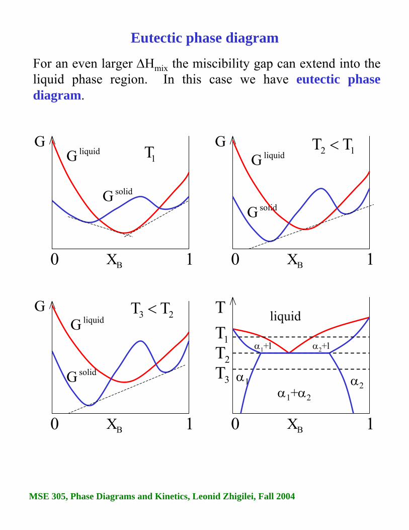
Eutectic phase diagram

For an even larger ∆Hmix the miscibility gap can extend into the liquid phase region. In this case we have eutectic phase diagram.

solidG

liquidG 1T

BX 10

G

solidG

liquidG12 TT <

BX 10

G

T

BX 10

3T

1T2T

liquid

α1α1+α2

solidG

liquidG23 TT <

BX 10

G

α2

α1+l α2+l


Eutectic phase diagram with different crystal structures of pure phases

A similar eutectic phase diagram can result if pure A and B havedifferent crystal structures.

1T

BX 10

G12 TT <

T

BX 10

3T

1T

2T

liquid

α

α + β

β

βα

liquid

BX 10

G

β α

liquid

23 TT <

BX 10

G

β α

liquid

α+l β+l


Eutectic systems - alloys with limited solubility (I)

Three single phase regions (α - solid solution of Ag in Cu matrix, β = solid solution of Cu in Ag matrix, L - liquid)

Three two-phase regions (α + L, β +L, α +β)

Solvus line separates one solid solution from a mixture of solid solutions. Solvus line shows limit of solubility

Copper – Silver phase diagram

liquid

α + β

Solidus

Liquidus

SolvusTem

pera

ture

, °C

Composition, wt% Ag


Eutectic or invariant point - Liquid and two solid phases co-exist in equilibrium at the eutectic composition CE and the eutectic temperature TE.

Eutectic isotherm - the horizontal solidus line at TE.

Eutectic reaction – transition between liquid and mixture of two solid phases, α + β at eutectic concentration CE.

The melting point of the eutectic alloy is lower than that of the components (eutectic = easy to melt in Greek).

Lead – Tin phase diagram

Invariant or eutectic point

Eutectic isotherm

Eutectic systems - alloys with limited solubility (II)Te

mpe

ratu

re, °

C

Composition, wt% Sn


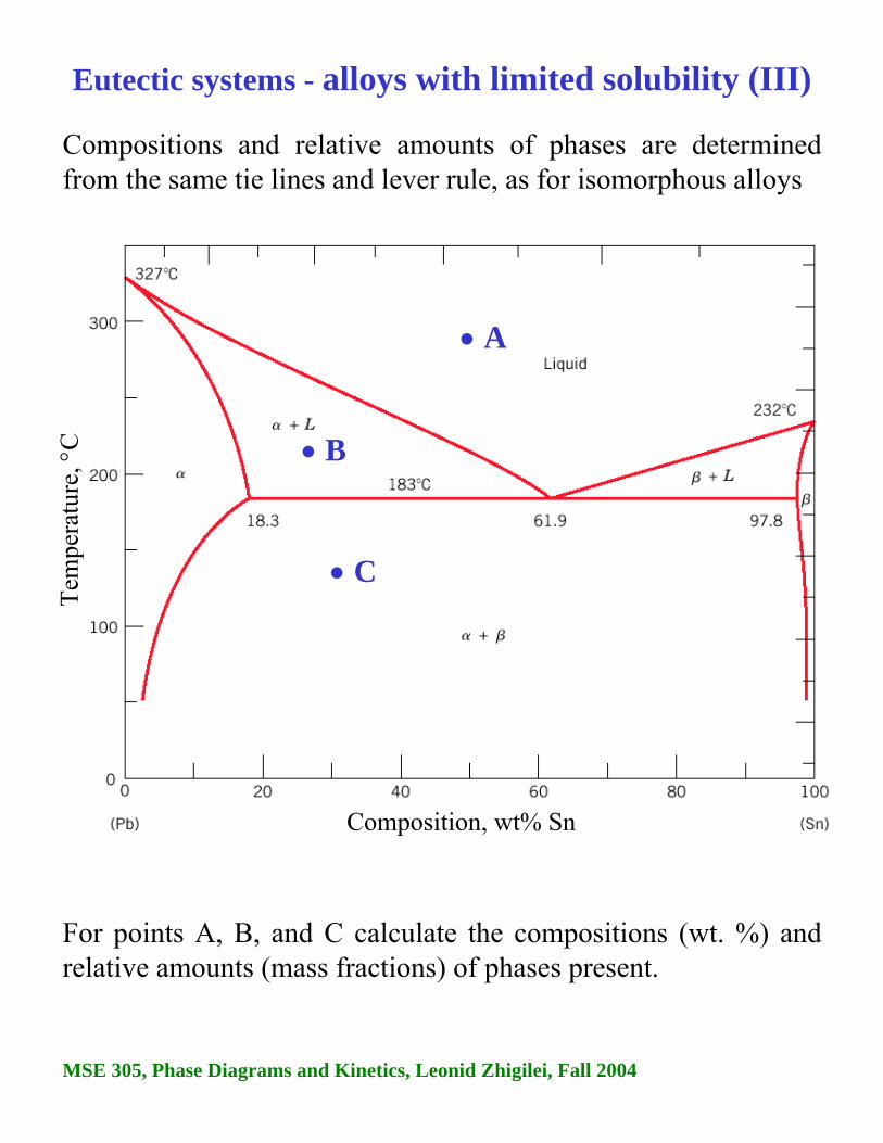
Compositions and relative amounts of phases are determined from the same tie lines and lever rule, as for isomorphous alloys

• C

For points A, B, and C calculate the compositions (wt. %) and relative amounts (mass fractions) of phases present.

• B

• A

Eutectic systems - alloys with limited solubility (III)

Composition, wt% Sn

Tem

pera

ture

, °C


Development of microstructure in eutectic alloys (I)

Several different types of microstructure can be formed in slow cooling an different compositions. Let’s consider cooling of liquid lead – tin system as an example.

In the case of lead-rich alloy (0-2 wt. % of tin) solidification proceeds in the same manner as for isomorphous alloys (e.g. Cu-Ni) that we discussed earlier.

L → α +L→ α

Composition, wt% Sn

Tem

pera

ture

, °C


Development of microstructure in eutectic alloys (II)

At compositions between the room temperature solubility limit and the maximum solid solubility at the eutectic temperature, βphase nucleates as the α solid solubility is exceeded upon crossing the solvus line.

L

α +L

α

α +β

Composition, wt% Sn

Tem

pera

ture

, °C


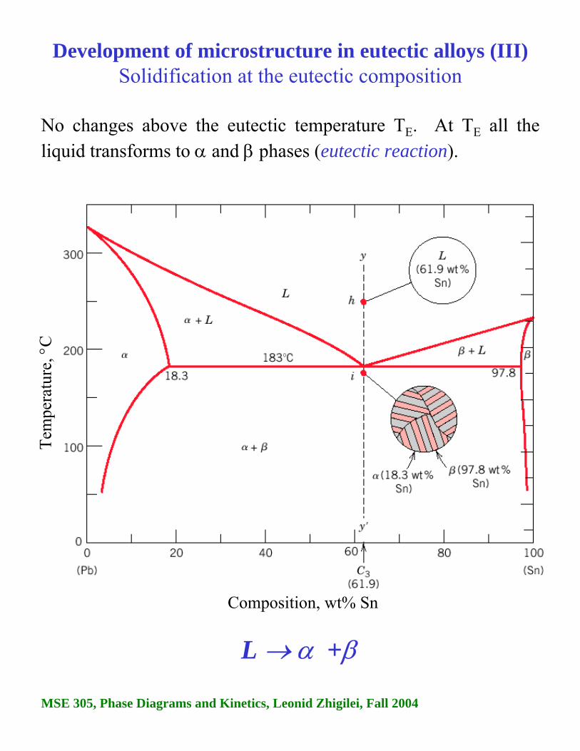
No changes above the eutectic temperature TE. At TE all the liquid transforms to α and β phases (eutectic reaction).

L → α +β

Development of microstructure in eutectic alloys (III)Solidification at the eutectic composition

Composition, wt% Sn

Tem

pera

ture

, °C


Development of microstructure in eutectic alloys (IV)Solidification at the eutectic composition

Compositions of α and β phases are very different → eutectic reaction involves redistribution of Pb and Sn atoms by atomic diffusion (we will learn about diffusion in the last part of this course). This simultaneous formation of α and β phases result in a layered (lamellar) microstructure that is called eutectic structure.

Formation of the eutectic structure in the lead-tin system.In the micrograph, the dark layers are lead-reach α phase, the

light layers are the tin-reach β phase.


Development of microstructure in eutectic alloys (V) Compositions other than eutectic but within the range of

the eutectic isotherm

Primary α phase is formed in the α + L region, and the eutectic structure that includes layers of α and β phases (called eutectic αand eutectic β phases) is formed upon crossing the eutectic isotherm.

L → α + L → α +β

Composition, wt% Sn

Tem

pera

ture

, °C


Development of microstructure in eutectic alloys (VI)

Microconstituent – element of the microstructure having a distinctive structure. In the case described in the previous page, microstructure consists of two microconstituents, primary αphase and the eutectic structure.

Although the eutectic structure consists of two phases, it is a microconstituent with distinct lamellar structure and fixed ratio of the two phases.


How to calculate relative amounts of microconstituents?

Eutectic microconstituent forms from liquid having eutectic composition (61.9 wt% Sn)

We can treat the eutectic as a separate phase and apply the lever rule to find the relative fractions of primary α phase (18.3 wt% Sn) and the eutectic structure (61.9 wt% Sn):

We = P / (P+Q) (eutectic) Wα’ = Q / (P+Q) (primary)

Composition, wt% Sn

Tem

pera

ture

, °C


How to calculate the total amount of α phase (both eutectic and primary)?

Fraction of α phase determined by application of the lever rule across the entire α + β phase field:

Wα = (Q+R) / (P+Q+R) (α phase)

Wβ = P / (P+Q+R) (β phase)

Composition, wt% Sn

Tem

pera

ture

, °C


Binary solutions with ∆Hmix < 0 - orderingIf ∆Hmix < 0 bonding becomes stronger upon mixing → melting point of the mixture will be higher than the ones of the pure components. For the solid phase strong interaction between unlike atoms can lead to (partial) ordering → |∆Hmix| can become larger than |ΩXAXB| and the Gibbs free energy curve for the solid phase can become steeper than the one for liquid.

αG

liquidG

1T

BX 10

23 TT < T

BX 103T

1T

2T

GG

liquid

α

α`

liquidG

BX 10

12 TT <

GliquidG

BX 10

αG

αG

α`G

At low temperatures, strong attraction between unlike atoms can lead to the formation of ordered phase α`.


Binary solutions with ∆Hmix < 0 - intermediate phasesIf attraction between unlike atoms is very strong, the ordered phase may extend up to the liquid.

T

BX 10

liquid

α

βα + β

γ

β + γ

In simple eutectic systems, discussed above, there are only two solid phases (α and β) that exist near the ends of phase diagrams.

Phases that are separated from the composition extremes (0% and 100%) are called intermediate phases. They can have crystal structure different from structures of components A and B.


∆Hmix<0 - tendency to form high-melting point intermediate phase

T

BX 10

liquid

α

α`

T

BX 10

liquid

α β

α + βγ

β + γ

T

BX 10

liquid

α

Increasing negative ∆Hmix


Phase diagrams with intermediate phases: example

Example of intermediate solid solution phases: in Cu-Zn, α andη are terminal solid solutions, β, β’, γ, δ, ε are intermediate solid solutions.


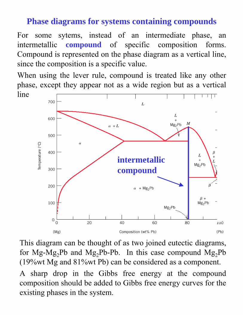
Phase diagrams for systems containing compoundsFor some sytems, instead of an intermediate phase, an intermetallic compound of specific composition forms. Compound is represented on the phase diagram as a vertical line,since the composition is a specific value. When using the lever rule, compound is treated like any other phase, except they appear not as a wide region but as a verticalline

This diagram can be thought of as two joined eutectic diagrams, for Mg-Mg2Pb and Mg2Pb-Pb. In this case compound Mg2Pb (19%wt Mg and 81%wt Pb) can be considered as a component. A sharp drop in the Gibbs free energy at the compound composition should be added to Gibbs free energy curves for the existing phases in the system.

intermetallic compound


Eutectoid Reactions

The eutectoid (eutectic-like in Greek) reaction is similar to the eutectic reaction but occurs from one solid phase to two new solid phases.

Eutectoid structures are similar to eutectic structures but are much finer in scale (diffusion is much slower in the solid state).

Upon cooling, a solid phase transforms into two other solid phases (δ ↔ γ + ε in the example below)

Looks as V on top of a horizontal tie line (eutectoid isotherm) in the phase diagram.

Eutectoid

Cu-Zn


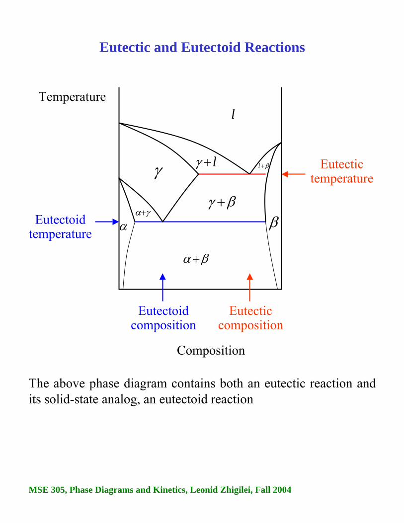
Eutectic and Eutectoid Reactions

The above phase diagram contains both an eutectic reaction and its solid-state analog, an eutectoid reaction

α

βα +

β

l+γ

βγ +γα+

β+lγ

lTemperature

Eutectic temperature

Eutectoid temperature

Eutectoid composition

Eutecticcomposition

Composition


Peritectic Reactions

A peritectic reaction - solid phase and liquid phase will together form a second solid phase at a particular temperature and composition upon cooling - e.g. L + α ↔ β

These reactions are rather slow as the product phase will form at the boundary between the two reacting phases thus separating them, and slowing down any further reaction.

Peritectoid is a three-phase reaction similar to peritectic but occurs from two solid phases to one new solid phase (α + β = γ).

Tem

pera

ture

liquid+α

βα +β liquid+β

liquid


Example: The Iron–Iron Carbide (Fe–Fe3C) Phase Diagram

In their simplest form, steels are alloys of Iron (Fe) and Carbon (C). The Fe-C phase diagram is a fairly complex one, but we will only consider the steel part of the diagram, up to around 7% Carbon.


Phases in Fe–Fe3C Phase Diagram

α-ferrite - solid solution of C in BCC Fe• Stable form of iron at room temperature. • The maximum solubility of C is 0.022 wt%• Transforms to FCC γ-austenite at 912 °C

γ-austenite - solid solution of C in FCC Fe• The maximum solubility of C is 2.14 wt %. • Transforms to BCC δ-ferrite at 1395 °C • Is not stable below the eutectic temperature

(727 ° C) unless cooled rapidly

δ-ferrite solid solution of C in BCC Fe• The same structure as α-ferrite• Stable only at high T, above 1394 °C• Melts at 1538 °C

Fe3C (iron carbide or cementite)• This intermetallic compound is metastable, it remains

as a compound indefinitely at room T, but decomposes (very slowly, within several years) into α-Fe and C (graphite) at 650 - 700 °C

Fe-C liquid solution


A few comments on Fe–Fe3C system

C is an interstitial impurity in Fe. It forms a solid solution with α, γ, δ phases of iron

Maximum solubility in BCC α-ferrite is limited (max. 0.022 wt% at 727 °C) - BCC has relatively small interstitial positions

Maximum solubility in FCC austenite is 2.14 wt% at 1147 °C -FCC has larger interstitial positions

Mechanical properties: Cementite is very hard and brittle - can strengthen steels. Mechanical properties also depend on the microstructure, that is, how ferrite and cementite are mixed.

Magnetic properties: α -ferrite is magnetic below 768 °C, austenite is non-magnetic

Classification. Three types of ferrous alloys:• Iron: less than 0.008 wt % C in α−ferrite at room T

• Steels: 0.008 - 2.14 wt % C (usually < 1 wt % )α-ferrite + Fe3C at room T

• Cast iron: 2.14 - 6.7 wt % (usually < 4.5 wt %)


Eutectic and eutectoid reactions in Fe–Fe3C

Eutectoid: 0.76 wt%C, 727 °C

γ(0.76 wt% C) ↔ α (0.022 wt% C) + Fe3C

Eutectic: 4.30 wt% C, 1147 °C

L ↔ γ + Fe3C

Eutectic and eutectoid reactions are very important in heat treatment of steels


Development of Microstructure in Iron - Carbon alloys

Microstructure depends on composition (carbon content) and heat treatment. In the discussion below we consider slow cooling in which equilibrium is maintained.

Microstructure of eutectoid steel (I)


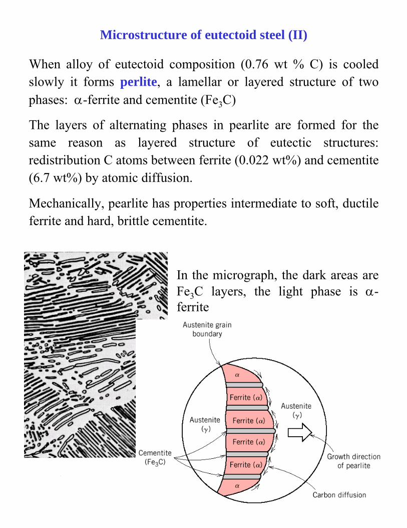
When alloy of eutectoid composition (0.76 wt % C) is cooled slowly it forms perlite, a lamellar or layered structure of two phases: α-ferrite and cementite (Fe3C)

The layers of alternating phases in pearlite are formed for the same reason as layered structure of eutectic structures: redistribution C atoms between ferrite (0.022 wt%) and cementite(6.7 wt%) by atomic diffusion.

Mechanically, pearlite has properties intermediate to soft, ductile ferrite and hard, brittle cementite.

Microstructure of eutectoid steel (II)

In the micrograph, the dark areas are Fe3C layers, the light phase is α-ferrite


Compositions to the left of eutectoid (0.022 - 0.76 wt % C) hypoeutectoid (less than eutectoid -Greek) alloys.

γ → α + γ → α + Fe3C

Microstructure of hypoeutectoid steel (I)


Hypoeutectoid alloys contain proeutectoid ferrite (formed above the eutectoid temperature) plus the eutectoid perlite that contain eutectoid ferrite and cementite.

Microstructure of hypoeutectoid steel (II)


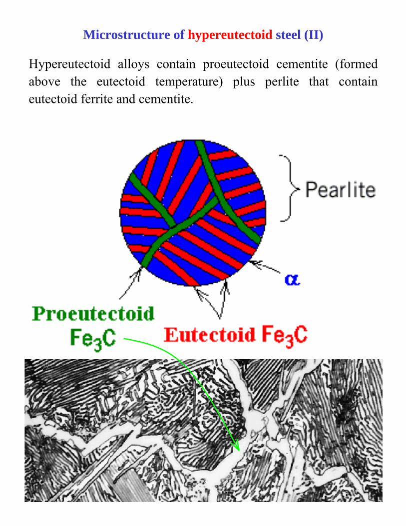
Compositions to the right of eutectoid (0.76 - 2.14 wt % C) hypereutectoid (more than eutectoid -Greek) alloys.

γ → γ + Fe3C → α + Fe3C

Microstructure of hypereutectoid steel (I)


Microstructure of hypereutectoid steel


Hypereutectoid alloys contain proeutectoid cementite (formed above the eutectoid temperature) plus perlite that contain eutectoid ferrite and cementite.

Microstructure of hypereutectoid steel (II)


How to calculate the relative amounts of proeutectoid phase (α or Fe3C) and pearlite?

Application of the lever rule with tie line that extends from the eutectoid composition (0.75 wt% C) to α – (α + Fe3C) boundary (0.022 wt% C) for hypoeutectoid alloys and to (α + Fe3C) – Fe3C boundary (6.7 wt% C) for hipereutectoid alloys.

Fraction of α phase is determined by application of the lever rule across the entire (α + Fe3C) phase field:


Example for hypereutectoid alloy with composition C1

Fraction of pearlite:

WP = X / (V+X) = (6.7 – C1) / (6.7 – 0.76)

Fraction of proeutectoid cementite:

WFe3C = V / (V+X) = (C1 – 0.76) / (6.7 – 0.76)


Let’s consider a simple one-component system.

The Gibbs phase rule (I)

liquidsolid

gas

T

P

In the areas where only one phase is stable both pressure and temperature can be independentlyvaried without upsetting the equilibrium → there are 2 degrees of freedom.

Along the lines where two phases coexist in equilibrium, only one variable can be independently varied without upsetting the two-phase equilibrium (P and T are related by the Clapeyronequation) → there is only one degree of freedom.

At the triple point, where solid liquid and vapor coexist any change in P or T would upset the three-phase equilibrium →there are no degrees of freedom.

In general, the number of degrees of freedom, F, in a system that contains C components and can have Ph phases is given by the Gibbs phase rule:

2PhCF +−=


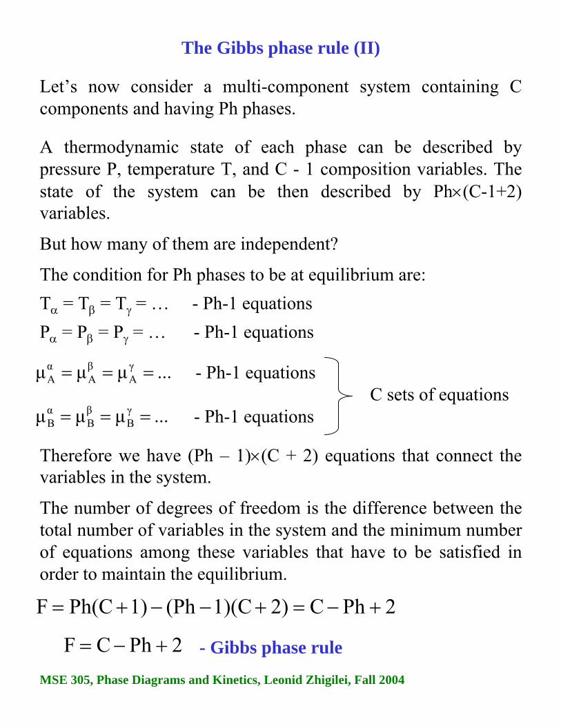
Let’s now consider a multi-component system containing C components and having Ph phases.

The Gibbs phase rule (II)

A thermodynamic state of each phase can be described by pressure P, temperature T, and C - 1 composition variables. The state of the system can be then described by Ph×(C-1+2) variables.

But how many of them are independent?

The condition for Ph phases to be at equilibrium are:Tα = Tβ = Tγ = … - Ph-1 equationsPα = Pβ = Pγ = … - Ph-1 equations

- Gibbs phase rule

2PhC2)1)(C(Ph1)Ph(CF +−=+−−+=

...µµµ γA

βA

αA === - Ph-1 equations

...µµµ γB

βB

αB === - Ph-1 equations

C sets of equations

Therefore we have (Ph – 1)×(C + 2) equations that connect the variables in the system.

The number of degrees of freedom is the difference between the total number of variables in the system and the minimum number of equations among these variables that have to be satisfied in order to maintain the equilibrium.

2PhCF +−=


In one-phase regions of the phase diagram T and XB can be changed independently.

In two-phase regions, F = 1. If the temperature is chosen independently, the compositions of both phases are fixed.

Three phases (L, α, β) may be in equilibrium only at a few points along the eutectic isotherm (F = 0).

The Gibbs phase rule – example (an eutectic systems)

2PhCF +−=

1PhCF +−=

constP =

Ph3F −=

2C =


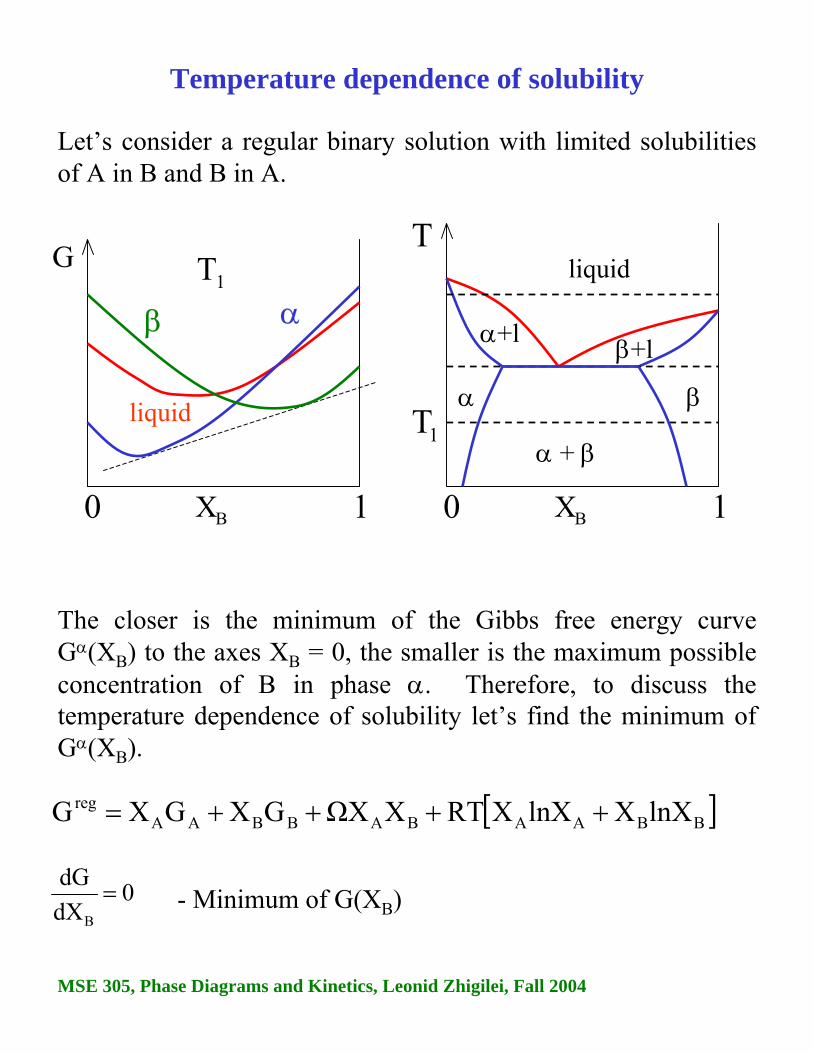
Temperature dependence of solubility

Let’s consider a regular binary solution with limited solubilitiesof A in B and B in A.

The closer is the minimum of the Gibbs free energy curve Gα(XB) to the axes XB = 0, the smaller is the maximum possible concentration of B in phase α. Therefore, to discuss the temperature dependence of solubility let’s find the minimum of Gα(XB).

T

BX 10

1T

liquid

α

α + β

β

1T

BX 10

G

β α

liquid

α+l β+l

[ ]BBAABABBAAreg lnXXlnXXRTXΩXGXGXG ++++=

0dXdG

B

= - Minimum of G(XB)


Temperature dependence of solubility (II)

( ) ( ) ( ) ( )[ ]BBBBBBBBAB lnXXX-1lnX-1RTXX-1GXGX-1 ++Ω++=

( ) ( )( ) =⎥

⎦

⎤⎢⎣

⎡++−+−Ω++=

B

BB

B

BBBBA

B XXlnX

X-1X-1X-1ln-RTX 2ΩG-G

dXdG

( )[ ]=++−Ω++= BBBBA lnXX-1ln-RTX 2ΩG-G

Solid solubility of B in α increases exponentially with temperature

[ ]BBAABABBAAreg lnXXlnXXRTXΩXGXGXG ++++=

( ) ( ) 0XRTlnG-GX-1

XRTln2X1G-G BABB

BBAB =+Ω+≈⎟⎟

⎠

⎞⎜⎜⎝

⎛+−Ω+=

if XB is small (XB → 0) Minimum of G(XB)

⎟⎠⎞

⎜⎝⎛ Ω+−−≈

RTGGexpX AB

B


Multicomponent systems (I)

The approach used for analysis of binary systems can be extended to multi-component systems.

Representation of the composition in a ternary system (the Gibbstriangle). The total length of the red lines is 100% :

XA +XB + XC =1

wt. %

wt. %

wt. %


Multicomponent systems (II)

The Gibbs free energy surfaces (instead of curves for a binary system) can be plotted for all the possible phases and for different temperatures.

The chemical potentials of A, B, and C of any phase in this system are given by the points where the tangential plane to the free energy surfaces intersects the A, B, and C axis.

G


Multicomponent systems (III)A three-phase equilibrium in the ternary system for a given temperature can be derived by means of the tangential plane construction.

Eutectic point: four-phase equilibrium between α, β, γ, and liquid

G

α β

γ

For two phases to be in equilibrium, the chemical potentials should be equal, that is the compositions of the two phases in equilibrium must be given by points connected by a common tangential plane (e.g. l and m).

The relative amounts of phases are given by the lever rule (e.g.using tie-line l-m).

A three phase triangle can result from a common tangential planesimultaneously touching the Gibbs free energies of three phases (e.g. points x, y, and z).


An example of ternary system

The ternary diagram of Ni-Cr-Fe. It includes Stainless Steel (wt.% of Cr > 11.5 %, wt.% of Fe > 50 %) and Inconeltm (Nickel based super alloys). Inconel have very good corrosion resistance, but are more expensive and therefore used in corrosive environments where Stainless Steels are not sufficient (Piping on Nuclear Reactors or Steam Generators).


Another example of ternary phase diagram: oil – water – surfactant system

Surfactants are surface-active molecules that can form interfaces between immiscible fluids (such as oil and water). A large number of structurally different phases can be formed, such as droplet, rod-like, and bicontinuous microemulsions, along with hexagonal, lamellar, and cubic liquid crystalline phases.

Drawing by Carlos Co, University of Cincinnati


SummaryElements of phase diagrams:

α + ββα

L

α + ββα

γ

α + Lα

βL

Eutectic (L → α + β)

Eutectoid (γ → α + β)

Peritectic (α + L → β)

α + βα

γβ

Peritectoid (α + β → γ)

Compound, AnBm

Make sure you understand language and concepts:

Common tangent constructionSeparation into 2 phasesEutectic structure Composition of phasesWeight and atom percentMiscibility gapSolubility dependence on TIntermediate solid solution Compound Isomorphous Tie line, Lever ruleLiquidus & Solidus lines Microconstituent Primary phaseSolvus line, Solubility limitAustenite, Cementite, FerritePearliteHypereutectoid alloy Hypoeutectoid alloyTernery alloysGibbs phase rule

A useful link:http://www.soton.ac.uk/~pasr1/index.htm

binary phase diagrams -...

Documents