ESTIMATION OF SITE-SPECIFIC ELECTRICITY

CONSUMPTION IN THE ABSENCE OF METER READINGS:

AN EMPIRICAL EVALUATION OF PROPOSED METHODS

David L. Ryan and Denise Young

April 2007

CBEEDAC 2007–RP-05

DISCLAIMER The views and analysis contained in this paper are the sole responsibility of the authors, and should not be attributed to any agency associated with CBEEDAC, including EPCOR Distribution Inc (EDI).

Executive Summary

The objective of this study is to describe, review and empirically evaluate the relative performance of alternative methodologies that may be used to estimate electricity consumption for individual sites in periods when no actual meter reading is undertaken. The empirical analysis is based on a random sample of approximately 30,000 sites drawn from the customer base of EPCOR Distribution Inc. (EDI) in Edmonton, Alberta. Separate sub-samples were obtained for residential, small commercial, and medium commercial sites, with the data pertaining to metering cycles over the period from January 2001 to mid 2004.

Five estimation methodologies are used to estimate electricity consumption over metering cycles. The estimates from these methodologies are compared to actual consumption, providing a measure of the error that occurs in the estimation process. Various evaluation criteria are applied to these errors in order to summarize the performance of each estimation methodology in aggregate and over different types of sites (residential, small commercial, and medium commercial) and over different time periods. These evaluation criteria include the average estimation error, the root mean square percentage error, as well as other criteria which may better reflect the disenchantment that customers might experience should they be invoiced for overestimates. These potential ‘disenchantment’ effects are captured via the proportion of overestimates that are large, as well as the proportion of sites that experience frequent large overestimates.

Our findings indicate that no single estimation method is better in all circumstances or according to all criteria. The method currently used by EDI, which is based on information from the immediately preceding metering cycle, performs best for residential sites and also performs well for small commercial sites. It does not perform as well for medium commercial sites, although the sub-sample of observations used in our analysis is much smaller for this type of site. An alternative method that is also based on information from the immediately preceding metering cycle also performs well in our data set, and in some cases does better than or as well as the EDI method. However, particularly for small and medium commercial sites, other estimation methods that utilize electricity consumption history from the same period in the previous year perform better according to some evaluation criteria. Our analysis also indicates that the relative performance of the various estimation methodologies is somewhat sensitive to the sample that is used in the evaluation. Nevertheless, for residential sites, the two methods that form estimates of consumption based on information from the immediately preceding meter cycle generally perform the best. An examination of performance across different years or months reveals that no single estimation method performs well in all cases. For residential sites, the EDI method performs well regardless of the particular year, but not in all months. The EDI method is frequently outperformed by an alternative method (that is also based on information from the previous meter cycle). Interestingly, both these methods exhibit strong seasonal patterns, tending to overestimate in some months and underestimate in others, although the over- and under-estimation periods differ for different types of sites. This suggests that the performance of these methods may be enhanced by including additional seasonal information.

i

In terms of the evaluation criteria related to potential customer ‘disenchantment’, the EDI method has the lowest rate of substantial overestimates for residential sites of all the estimation methods that were considered, although approximately 10% of all estimates exceed actual values by more than 25%, even for the best performing method. In general, for all types of sites, the methods that utilize information from the previous meter cycle tend to yield better estimates according to this criterion than those based on information from the same period in the previous year. In terms of the frequency with which particular sites experience overestimates of their electricity consumption, these same two methods tend to result in smaller proportions of sites that receive overestimates in a large proportion of cases. An empirical examination of the inclusion of proxies for variations in weather conditions and other seasonal factors in the estimation process indicates that these adjustments do not always improve the ability of the various estimation methods to provide accurate estimates of electricity consumption.

ii

Table of Contents

Executive Summary …………………………………………………………………… i List of Tables …………………………………………………………………………. v List of Figures ………………………………………………………………………… vi

1. Introduction …………………………………………………………………… 1

2. Background …………………………………………………………………… 3

3. Data …………………………………………………………………………… 6

3.1 Data Structure............................................................................................... 6 3.2 Data Requirements for Estimation Methods ....…………………………… 6 3.3 Sample Sizes for Residential, Small Commercial and Medium Commercial

Data Sets…………………………………………………………………… 7

4. Methodology ………………………………………………………………….. 9

4.1 Methods based on information from the immediately preceding metering period ……………………………………………………………………… 9

4.1.1 Method A …………………………………………………………… 9

4.1.2 Method B …………………………………………………………… 10

4.2 Methods based on information from the same general period in the

previous year …………………………………………………..…………. 11

4.2.1 Method C …………………………………………………………… 11

4.2.2 Method D ....………………………………………………………… 13

4.2.3 Method E ....………………………………………………………… 13

5. Results ………………………………………………………………………… 16

5.1 Evaluation of Electricity Consumption Estimates ………………………… 16

5.1.1 Average Estimation Error (AEE) …………………………………… 16

5.1.2 Root Mean Square Percentage Error (RMSPE) …………………….. 16

5.1.3 Other Measures ……………………………………………………… 17

5.1.3.1 Proportion of Large Consumption Overestimates …………… 17

5.1.3.2 Proportion of Sites with Frequently Large Overestimates …... 18

5.2 Aggregate Results ……………………………….………………………… 19

5.2.1 Residential …………………………………………………………… 20

5.2.2 Small Commercial …………………………………………………… 20

5.2.3 Medium Commercial ………………………………………………… 20

iii

5.3 Robustness of Aggregate Results ……………………………….…………. 21

5.4 Patterns in Estimation Accuracy over Time …………………….…………. 21

5.4.1 Residential …………………………………………………………… 22

5.4.2 Small Commercial …………………………………………………… 22

5.4.3 Medium Commercial ………………………………………………… 23

5.5 Proportion of Large Consumption Overestimates …..………………….….. 23

5.5.1 Residential Customers …..…………………………………………… 23

5.5.2 Small Commercial Customers………………………………………… 24

5.5.3 Medium Commercial Customers ……………………………………… 24

5.6 Proportion of Sites with Frequently Large Overestimates ..……………..…. 24

6. Proxied Adjustments for Weather and Other Seasonal Factors ………………… 26

7. Summary and Conclusions ……………………………………………………. 28

References …………………………………………………………………………….. 30

iv

List of Tables

Table 1a: Aggregate Results – Residential (26,990 sites) ……………………………… 31

Table 1b: Aggregate Results – Small Commercial (2,696 sites) ………………………. 31

Table 1c: Aggregate Results – Medium Commercial (300 sites) ……………………… 32

Table 2a: Aggregate Results –Residential Sub-Sample #1 (2,632 sites ………………. 33

Table 2b: Aggregate Results –Residential Sub-Sample #2 (2,630 sites) ………………. 33

Table 2c: Aggregate Results –Residential Sub-Sample #3 (2,627 sites) ……………… 34

Table 2d: Aggregate Results –Residential Sub-Sample #4 (2,618 sites) ……………… 34

Table 2e: Aggregate Results –Residential Sub-Sample #5 (2,619 sites) ……………… 35

Table 2f: Aggregate Results –Residential Sub-Sample #6 (2,623 sites) ……………… 35

Table 2g: Aggregate Results –Residential Sub-Sample #7 (2,623 sites) ……………… 36

Table 2h: Aggregate Results –Residential Sub-Sample #8 (2,625 sites) ……………… 36

Table 2i: Aggregate Results –Residential Sub-Sample #9 (2,624 sites) ……………… 37

Table 2j: Aggregate Results –Residential Sub-Sample #10 (3,369 sites) ……………. 37

Table 3a: Variations in RMSPE over Time – Residential …………………………… 38

Table 3b: Variations in Average Estimation Error over Time – Residential ………… 38

Table 3c: Variations in RMSPE over Time – Small Commercial …………………… 39

Table 3d: Variations in Average Estimation Error over Time – Small Commercial … 39

Table 3e: Variations in RMSPE over Time – Medium Commercial ………………… 40

Table 3f: Variations in Average Estimation Error over Time – Medium Commercial .. 40

Table 4a: Proportion of Overestimates by Year: Residential …………………………. 41

Table 4b: Proportion of Overestimates by Time of Year: Residential ……………….. 42

Table 4c: Proportion of Overestimates by Year: Small Commercial ………………… 44

Table 4d: Proportion of Overestimates by Time of Year: Small Commercial ………. 45

Table 4e: Proportion of Overestimates by Year: Medium Commercial ……………… 47

Table 4f: Proportion of Overestimates by Time of Year: Medium Commercial …….. 48

Table 5a: Percentage of Sites with Frequent Overestimates – Residential ………….. 50

Table 5b: Percentage of Sites with Frequent Overestimates – Small Commercial ….. 51

Table 5c: Percentage of Sites with Frequent Overestimates – Medium Commercial .. 52

Table 6: Comparison of Adjusted and Unadjusted Estimates for Residential Customers, 2003-2004 ………………………………………………………. 53

v

vi

List of Figures

Figure 1: A schematic of Metering at a Particular Site ………………………………… 3

Figure 2: Number of Sites, EDI, 2001-2004 …………………………………………... 7

1. Introduction

Since reading of electricity meters is an expensive and time-consuming undertaking, in most jurisdictions meters are not read for each and every invoice that is issued to a customer. Rather, many of these invoices are based on estimated rather than actual electricity consumption. In the case of Epcor Distribution Inc. (EDI), invoices for a substantial portion of the customer base are issued monthly while the meters for these customers are generally read bi-monthly. Hence, for residential and small commercial customers in particular, every second electricity invoice is based on estimated - rather than actual – electricity consumption. Although electricity consumption for an individual site is not known in the absence of a meter reading, total electricity consumption (or net system load, NSL) for all sites since the last meter reading for any given site is known. This NSL information is used by EDI, along with site-specific information from the previous meter reading at a site, to estimate electricity consumption for individual sites for billing periods with no available meter reading. On average, these estimates should be accurate in that the sum of estimated electricity consumption over these sites during the estimation period can be set to equal actual consumption for this same period. From the point of view of the electricity supplier there would appear to be no aggregate gain or loss involved in incorrectly estimating electricity consumption for particular individual sites, since any overestimates can be exactly offset by equivalent underestimates for other sites.1 When electricity prices are constant, there should also be little overall impact on electricity consumers arising from minor inaccuracies due to the estimation of electricity consumption in periods when no actual meter reading is undertaken. Regardless of the estimate that is made, when the next actual meter reading is taken, actual consumption pertaining to the entire period between meter readings (the metering cycle) is known. Since this period includes the sub-period for which consumption had previously been estimated, billing of the difference between this actual consumption figure and the previously estimated amount means that the electricity consumer has been correctly billed for the amount of their electricity consumption over the entire metering cycle. Thus, over-estimation of consumption in the first sub-period simply involves a temporary loan from the electricity consumer to the electricity supplier, while under-estimation results in a temporary loan in the reverse direction. Provided the sum of estimated electricity consumption over these sites during the estimation period is set equal to actual consumption for this same period, there is no net revenue transfer in either direction. However, (a subset of) consumers may be dissatisfied with the process if they are systematically subject to significantly overestimated bills. In this report, we describe and evaluate five basic methods of establishing electricity consumption estimates for individual sites in periods when no actual meter reading is

1 Note, however, that because all of the estimate factors for all sites are based on different periods of time, the sum of estimated consumption might be slightly more or less than actual consumption. Therefore there is normally UFE – unaccounted for energy – left over when the process ends.

1

undertaken. In addition to the method currently used by EDI, four other methods are evaluated, including those used by (or suggested for use in) other jurisdictions. Our evaluation of various estimation strategies is based on data pertaining to a sample of individual residential, small commercial, and medium commercial sites supplied by EDI, predominately in Edmonton, Alberta. The criteria that are selected are designed to compare the abilities of various estimation methods to accurately forecast electricity consumption according to a series of metrics. The measures that we consider are: the average difference between estimated and actual consumption, root mean square percentage error, and the proportion of observations for which large overestimates result from each estimation method. Due to the fact that actual consumption by individual sites is never known in building periods when meters are not read, our evaluation is based on a slight modification of actual practice. We form estimates of consumption pertaining to an entire metering cycle for each proposed method and compare these estimates to the known consumption over that cycle. The remainder of this report is organized as follows. Section 2 provides a framework for describing the various methods that are used to estimate electricity consumption, and identifies a general approach that can be used to evaluate the different methods. A description of the data and various summary statistics are contained in Section 3, while the various estimation methodologies that are evaluated are described and reviewed in Section 4. Section 5 describes and analyzes the main results that are obtained when the various estimation methodologies are used to estimate consumption in our sample of data. This section also contains a detailed description of the various criteria that are applied in our evaluation of the electricity consumption estimates obtained using the different estimation methodologies. Adjustments that could be made to the estimation methods to account for weather and other seasonal factors are considered briefly in Section 6. Section 7 summarizes and concludes.

2

2. Background

To provide a framework for describing the various methods that are used to estimate electricity consumption in periods when no meter reading is taken, as well as to identify the issues involved in evaluating alternative methods and the data that are required, it is convenient to consider the following schematic, which pertains to any particular site that receives invoices based on consumption estimates between meter readings.

Figure 1: A Schematic of Metering at a Particular Site

A B C D E actual estimate actual estimate actual meter meter meter read read read

A meter cycle refers to the period between consecutive meter reads such as from A to C, or from C to E. Actual consumption is known for these periods. The issue that is addressed in this report concerns the estimates that are made at points B and D, when no meter reading is obtained. At these points the customer is invoiced for the amount of electricity that has presumably been used since the previous meter read, that is, from A to B, or from C to D, respectively. While it is clearly desirable to estimate this consumption as accurately as possible, particularly in an era when prices may be changing frequently, the extent of any over- or under-estimate that may be made at B or D should have no long-term implications for the customer, since it will be corrected with the invoice that is issued following the next meter reading. For example, if the customer is estimated to have consumed “x” kWh of electricity from A to B, and at the next meter read at C it is found that they consumed “y” kWh in total between A and C, then if they are invoiced for “y-x” kWh consumption between B and C, they will have been charged correctly for their consumption over the complete meter cycle from A to C. Ideally, in order to evaluate the accuracy of the estimates that are made at points like B and D, estimated consumption for periods such as from A to B would be compared to actual consumption for those periods. Unfortunately, in the absence of meter readings, those actual consumption values can never be known. Therefore, it is necessary to use alternative measures to evaluate the accuracy of the estimates. One approach that has been used, and which will be considered in more detail in Section 4.1 is to express the estimated consumption of a particular site in the estimated period (say from A to B) as a share of total consumption in that period, since total consumption (that is, consumption by all sites) in the estimated period is known. Algebraically, this can be written in terms of the following relationship (where hats (^) over variables indicate estimated measures):

(1) AB

ABiAB

i NSLCsˆ

ˆ =

where is estimated consumption by site i over the period from A to B, ABiC

3

ABNSL is Net System Load over the period from A to B, which is actual aggregate consumption across all sites over the period from A to B, and

ABis is the estimated share of aggregate consumption over the period from A to B that is

attributable to site i.

Then, following the next meter reading, when actual consumption by that site over the meter cycle from A to C is known, the actual share of that site in the total consumption over the period from A to C can be calculated. Algebraically, this share can be written as:

(2) AC

ACiAC

i NSLCs =

where is actual consumption by site i over the period from A to C (so that estimated

consumption from B to C is given by ),

ACiC

ABi

ACi

BCi CCC ˆˆ −=

ACNSL is Net System Load over the period from A to C, which is actual aggregate consumption across all sites over the period from A to C, and

ACis is the actual share of aggregate consumption over the period from A to C that is

attributable to site i.

The extent to which the estimated share over A to B ( ) and the actual share over A to C ( ) differ can then be used as a measure of the inaccuracy of the estimate. Thus, for example, if these two shares were equal ( ), the estimate would be viewed as perfect. However, this measure of the (in)accuracy of the estimate is only useful if the share of total consumption attributable to a particular site is the same in every portion of a meter cycle, which is unlikely to be the case. In other words, even if , the estimate over the period from A to B might not have been accurate – it could be the case that over the estimate period from A to B the site actually consumed less than , so that their actual share for the period A to B was less than

, while in the remainder of the meter cycle, from B to C, they consumed more than , so that their share in the latter part of the meter cycle was greater than . Therefore, a comparison of these two shares does not provide an objective measure of the accuracy of the estimate in the period from A to B.

ABis

ACis

ABis

ACi

ABi ss =ˆ

ABis =ˆ

AB

ACis

iCBCiC

ACis

An alternative approach to evaluating various methods that might be used to estimate consumption in a period when a meter reading is not taken involves focusing solely on periods that involve actual meter readings. In this way, the estimates that are obtained for a particular period using the different estimation methods can be compared to actual outcomes for that same period. For example, in Figure 1, meter readings are taken at point C and at point E, so that actual consumption is known in the period A to C and in the period C to E. Now, for example, rather than estimating consumption for the period A to B using known information about a particular site prior to point A, as well as known information about aggregate measures, such as NSL, over the period from A to B, the estimates could be made for the entire period from A to C. In this case the estimate would be formed based on known information about a particular site prior to point A, as well as known information about aggregate measures, such as NSL, over the

4

period from A to C. In this way, the estimation that is undertaken over the period from A to C exactly mimics the estimation that would be done from A to B. However, now the estimate that is obtained for the entire meter cycle from A to C can be compared to the known value of actual consumption from A to C, thus providing an objective means of evaluating the accuracy of the estimation method. This is the method that is used in this report to assess the accuracy of various methods for estimating consumption in a period when no meter reading is taken.

5

3. Data

3.1 Data Structure: To evaluate different methods for estimating electricity consumption in periods when no meter reading is taken, data were obtained from EDI on a random sample of approximately 30,000 sites. These sites were drawn from EDI’s customer base of residential, small commercial, and medium commercial customers, with the data pertaining to metering cycles over the period from January 2001 to mid-2004. In order to implement the various methods, which are described in detail in the Sections 4.1 and 4.2, the following information was obtained for each site over a meter cycle, such as from A to C in Figure1:

• Start Date (hour, day, month, year) • End Date (hour, day, month, year) • Actual Consumption • NSL (aggregate consumption over all sites)2

From this information, the number of days and hours in the meter cycle were calculated, as well as the ratio of consumption by this site to total consumption by all sites over the same period (corresponding to the actual share in the previous descriptions). The data that are available for each site do not include the date/time at which consumption was estimated. However, for subsequent analysis, an end date for the estimate period – corresponding to a point such as B or D in Figure 1 – is assigned for each meter cycle for each site as the mid point of the meter cycle period. Although actual consumption is not known in this estimate period, the corresponding NSL is known, and this information was also recorded along with the end date and time for the estimate period.

ACis

The information that is described above was obtained for each site for every meter cycle starting at Jan 1, 2001. Initial meter cycles were often incomplete, and were therefore discarded from our sample. The resulting data set therefore contains complete information from a sequence of meter cycles for each site. Since the start date and end dates of a meter cycle differ across sites, and since not all sites consume electricity in every meter cycle, the number of complete meter cycles containing usable information varies across sites. 3.2 Data Requirements for Estimation Methods: Almost all of the methods that have been proposed or used to estimate electricity consumption in periods when no meter reading is taken make use of some aspect(s) of a site’s electricity consumption history. Therefore, for each meter cycle for each site it is necessary to assemble this electricity consumption history. As described in detail in the Section 4, for some estimation

2 Note that NSL is revised, possibly several times, as additional information becomes available. Since these revisions typically take several months, possibly even longer than one year, the only information that can be used for estimating consumption in periods when meters are not read is the initial estimate of NSL, which is the measure used here.

6

strategies the consumption history that is required pertains only to the immediately preceding meter cycle, but for others it pertains to the corresponding meter cycle in the preceding year, or the sequence of meter cycles since the corresponding meter cycle in the preceding year. As a result, for many meter cycles the electricity consumption history that would be required for some estimation methods cannot be obtained, in which case these meter cycles cannot be included in the empirical analysis. In addition to site-specific information, some methods that are used to estimate consumption make use of other particulars, such as weather-related variables, and information on the total number of sites that are included in NSL. Relevant weather variables were obtained for Edmonton, while EDI provided data on the number of sites included in NSL. Unfortunately, part way through the data period (May 2003), a clean-up of sites was performed, with a large number of sites (approximately 3.7%) removed from the database due to such factors as, for example, buildings that had been demolished, etc. However, it is not known if these sites that were omitted in May 2003 were not consuming electricity for the entire sample period, that is, since January 2001. It does appear from Figure 2 that the growth rate in the number of sites is approximately the same after the site clean-up as before, suggesting that these sites could probably also be excluded from the site count prior to May 2003.

Figure 2: Number of Sites, EDI, 2001-2004

270000

280000

290000

300000

310000

01/0

1/01

01/0

5/01

01/0

9/01

01/0

1/02

01/0

5/02

01/0

9/02

01/0

1/03

01/0

5/03

01/0

9/03

01/0

1/04

3.3 Sample Sizes for Residential, Small Commercial and Medium Commercial Data Sets: Since the medium commercial sites in the sample tend to be metered on approximately a monthly cycle, while most residential and small commercial sites are metered on an approximate two-month cycle, and since the electricity consumption characteristics of these different types of sites may differ, we treat these different types of sites separately in our analysis. For residential

7

customers, the sample includes information from 26,990 sites, consisting of 493,419 individual observations on meter-reading cycles. Once observations with zero consumption are eliminated, there are 26,973 sites remaining, comprising 489,451 observations, or an average of 18 usable meter cycles per site. On average, these residential meter-reading cycles span 58 days and involve consumption of 990.62 kWh. The small commercial data set consists of 61,955 meter-reading cycle observations pertaining to 2,696 sites. When observations with no consumption activity are removed, there are 2,681 sites remaining, with a total of 60,233 meter-reading cycle observations, an average of 22.5 usable meter cycles per site. These small commercial meter reading cycles span 46.4 days on average, with an average consumption of 3681.04 kWh. The medium commercial data set contains data from 300 active sites. There are 9,840 observations, 9,795 of which are from periods with non-zero activity, so that on average there are 32.5 usable meter reading cycles per site. This high number of cycles indicates that for this category of sites the meters are read almost every month at each site. This is reflected in the average meter cycle length of 31.46 days. Average consumption over these 9,795 meter-reading cycles is 21003.26 kWh. For various reasons, including missing values for other information required for estimation, and the need to construct electricity consumption histories for each meter cycle (which cannot be done for the first set of cycles for each site), fewer observations are actually used in the subsequent empirical analysis.

8

4. Methodology

Using the three samples of EDI data, we apply five main methods of estimating electricity consumption in periods when no meter reading is taken. Two of these methods utilize historical electricity consumption information from the previous metering period, while the remaining three utilize electricity consumption information from the same general period in the previous year (sometimes in conjunction with additional information from the period for which consumption is being estimated). As discussed previously, we generate estimates corresponding to the five methods for an entire meter cycle rather than just for part of a cycle, as is done in practice. This facilitates a comparison of the estimates that are produced with subsequent actual consumption data, so that the accuracy of the estimates can be assessed. It is possible that estimation over an entire meter cycle, which covers a longer period than is considered in practice may result in less reliable estimates. However, any resulting decrease in reliability should affect all estimation methods considered, so that there is no a priori expectation that this longer estimation period will affect the comparisons of accuracy across methods. The same evaluation criteria are applied to all methods: average difference between estimated and actual consumption, mean square percentage error, and the proportion of observations for which there are “large” overestimates. These criteria are described in more detail in Section 5.1. For all estimation methods, estimates are only formed for meter cycles that involve current consumption activity. 4.1 Methods based on information from the immediately preceding metering period Estimation methods that make use of electricity consumption history for a site in the immediately preceding metering period might be expected to provide accurate estimates of consumption in the current period in the sense that the immediately preceding period contains the most recent information that is available about electricity consumption at that site (both in terms of actual consumption and consumption relative to aggregate electricity consumption over all sites). The two methods considered here differ in terms of the information that is used from the previous period, and in the way this information is updated for the current period. 4.1.1 Method A One approach to estimating electricity consumption for a particular site in the current period utilizes information on consumption of electricity at that site in the immediately preceding metering period, as well as aggregate consumption (across all sites) in the current and immediately preceding periods. In the previous metering period, the difference between two consecutive meter readings, generally about 60 days apart, yields actual consumption for a particular site during that period. Total consumption by all cumulatively metered sites – Net System Load (NSL) – during that same period is also known. Using this information, the ratio of consumption by this one site to NSL can be calculated, thereby yielding the proportion of NSL attributable to this particular site during that previous period (the site’s usage factor). Algebraically:

9

(3) 1

1,1,

−

−− =

t

titi NSL

Cs

where is the usage factor for site i in period t-1 (the immediately preceding metering period),

1, −tis

1, −tiC is actual consumption by site i in period t-1,

1−tNSL is Net System Load in period t-1, which is actual aggregate consumption over all sites in the immediately preceding period.

Since NSL is also known for the period from the last actual meter read to the date when the estimate is to be made, multiplication of this site’s usage factor for the earlier period with the actual NSL for the current billing period yields an estimate of consumption at this site for the period since the last meter reading occurred. Algebraically,

(4) tt

tittiti NSLNSL

CNSLsEstimateA ⎟⎠⎞

⎜⎝⎛==

−

−−

1

1,1,,

where is the estimated electricity consumption by site i in period t, which is the current period – defined as the time since the last meter reading was taken,

tiEstimateA ,

1, −tis is the usage factor for site i in period t-1 (the immediately preceding period), as defined in equation (3),

tNSL is Net System Load in the period since the last meter read, which is actual aggregate consumption over all sites since the last meter reading at site i.

This is the method currently employed by EDI. The main advantage of this method is that it takes into account changes in total consumption between the previous period and the current period – if total consumption increases, then the sites are collectively consuming more electricity in the current period than in the previous period, and this will be reflected in increased estimates for each site. Conversely, if total consumption is lower in the current period than in the previous period, this will be reflected in lower estimates for each site. However, if total consumption changed because there are more or fewer sites included, or simply because certain (but not all) sites changed their consumption, this method will tend to overestimate electricity consumption in the current period for many sites and underestimate for many others. Furthermore, in this context, this problem of over- and under-estimation will occur whether aggregate consumption is increasing or decreasing. 4.1.2 Method B An alternative approach is to base the estimate of electricity consumption in the current period – that is, since the last meter reading – on the known levels of consumption per day at the same site in a previous period. This is known as an Average Daily Use (ADU) estimation method.3 In addition to ENMAX, ADU methods are used by Fortis in Alberta and by utilities in other

3 This estimation strategy is outlined in the ENMAX document “Reasonability of Estimation Approaches for Settlement and Billing”, dated August 31, 2004.

10

countries such as Western Massachusetts Electric (WME) and Detroit Edison (DTE Energy) in the U.S. and The Australian Gas Light Company (AGL) in Australia.4 Under this approach, consumption for the billing period can be estimated based on the immediately preceding period’s average daily consumption at the site as:

(5) titi

titi DaysDays

CEstimateB ,1,

1,, ⎟

⎠⎞

⎜⎝⎛=

−

−

where is the estimated electricity consumption by site i in period t, which is the current period – defined as the time since the last meter reading was taken,

tiEstimateB ,

1, −tiC is actual consumption by site i in period t-1,

1, −tiDays is the number of days between meter reads for site i in the previous meter cycle,

tiDays , is the number of days for site i in the current meter cycle (since the last meter read for this site).

The main difference between Method A and Method B is that with Method A it is assumed that a site’s share of electricity consumption in the previous period will also apply in the current period, while with Method B, it is assumed that the site’s daily consumption is the same in the current period as in the previous period. The main advantage of Method B is that it focuses on site-specific information. Its main disadvantage is that even if aggregate consumption over all sites changes – for example, due to changes in seasons, etc. – this will not be reflected in the electricity estimates that are formed for any site. Thus, this method would be expected to tend to overestimate electricity consumption for each site when aggregate consumption decreases, and underestimate it when aggregate consumption increases, unless these changes in aggregate consumption were solely due to a decrease or an increase in the number of sites, respectively. 4.2 Methods based on information from the same general period in the previous year The general methods considered above can also be implemented using data from the same period in the previous year, instead of in the immediately preceding metering period. This modification means that the estimates may be able to capture seasonal influences that are similar in size and timing from year to year. The generalizations to the previous methods are quite straightforward, as shown below. 4.2.1 Method C Some utilities, such as DTE Energy, use ADU strategies based on average daily consumption patterns corresponding to (approximately) the same time period in the previous year.5 Thus, this

4 See the Appendix for a selection of websites that describe billing/estimation practices for a cross-section of electric utilities. 5 See the description of the electricity consumption estimation process used by DTE Energy on the Detroit Edison and MichCon website at http://my.dteenergy.com/myAccount/meterRead.do.

11

method is a direct generalization of Method B in the previous section. In this case, the estimate is calculated as:

(6) titi

titi DaysDays

CEstimateC ,6,

6,, ⎟

⎠⎞

⎜⎝⎛=

−

−

where is the estimated electricity consumption by site i in period t, which is the current period – defined as the time since the last meter reading was taken,

tiEstimateC ,

6, −tiC is actual consumption by site i in period t-6, that is, six meter cycles previously,

6, −tiDays is the number of days between meter reads for site i in period t-6, that is, six meter cycles previously,

tiDays , is the number of days for site i in the current meter cycle (since the last meter read for this site).

Since, for residential and small commercial sites, a metering cycle is approximately 60 days, or two months, consumption measures from six meter cycles previously will approximately reflect consumption in the same period in the previous year. For medium commercial sites where there are generally 12 readings per year, and would be replaced in equation (6) by

and , respectively, so that the estimation method would again reflect consumption from a similar period approximately one year earlier.

6, −tiC 6, −tiDays

12, −tiC 12, −tiDays

One difficulty with implementing this method, and which applies also to any method that utilizes information pertaining to consumption in a similar period in the previous year, is that for various reasons meter readings are not always made on a regular schedule. For example, an unusual reading or some particular event may result in a residential meter being read every month for a period of several months before regular bi-monthly meter readings are resumed. Consequently, electricity consumption and other information from six periods ago (or 12 periods ago for medium commercial sites) may not represent consumption from approximately the same period in the previous year for all sites. To guard against this possibility, and therefore the possibility that estimates obtained in our analysis would not accurately reflect the quality of estimates that would normally be obtained using this method, certain restrictions were placed on data points when using this method. Specifically, data points were excluded from the sample unless the following criteria were met:

• the number of days elapsed since the beginning of the meter-reading interval 6 periods ago (or 12 periods ago for medium commercial sites) must be between 330 and 400 days, so that 6, −tiC and 6, −tiDays correspond to approximately the same ‘season’ in the previous year;

• the length of the meter-reading interval for the comparison period must differ by no more than 15 days from the estimation interval for the current period.

12

4.2.2 Method D Although, to our knowledge, not currently used by any utilities, Method A can also be adapted to incorporate information from the same period in the previous year. That is, the ‘usage factor’ applied to current aggregate consumption can be calculated as the share of total consumption attributable to a site from the same time period in the previous year rather than in the previous period. Thus, with this approach the estimate would be obtained using the following formula:

(7) tt

tittiti NSLNSL

CNSLsEstimateD ⎟⎠⎞

⎜⎝⎛==

−

−−

6

6,6,,

where is the estimated electricity consumption by site i in period t, which is the current period – defined as the time since the last meter reading was taken,

tiEstimateD ,

6, −tis is the usage factor for site i in period t-6, that is, six meter cycles previously, as defined by the term in parentheses in equation (7),

6, −tiC is actual consumption by site i in period t-6, that is, six meter cycles previously,

6−tNSL is Net System Load in period t-6, which is actual aggregate consumption over all sites in period t-6, that is, six meter cycles previously (based on meter cycles for site i),

tNSL is Net System Load in the period since the last meter read, which is actual aggregate consumption over all sites since the last meter reading at site i.

The data points that are employed in the empirical analysis to obtain consumption estimates using Method D are limited to those that satisfy the same restrictions as described previously for Method C. 4.2.3 Method E A variation of Methods C and D has been suggested in a recent report by Baraniecki and Koehn (2002).6 With this approach, the estimate of electricity consumption for a particular site in the next billing period is obtained by determining the percentage of that site’s annual consumption that occurred in (approximately) the same period in the previous year, and then applying that percentage to that site’s projected annual consumption for the current year. This approach involves a number of steps that can be described as follows: Step 1: Calculate weights that reflect the percentage of annual consumption by a particular site

(site i) for comparison periods in the previous year:

(8) ⎟⎠⎞

⎜⎝⎛

+++++=−−−−−−

−− )(1

7,6,5,4,3,2,

7,1,

titititititi

titi CCCCCC

CW

(9) ⎟⎠⎞

⎜⎝⎛

+++++=−−−−−−

−− )(2

7,6,5,4,3,2,

6,1,

titititititi

titi CCCCCC

CW

6 J.M. Baraniecki and S. Koehn “Proposed Billing Estimation Method Using Consumption Profiles”, Working Paper, EPCOR Energy Services Inc, November 2002.

13

where is actual consumption by site i in period t-k, that is, k meter cycles previously, where k = 2, 3, 4, 5,6, or 7.

ktiC −,

1,1 −tiW is a weight (0 < < 1) that indicates the proportion of the previous year’s electricity consumption by site i that was consumed in the same period in the previous year as the immediately preceding metering period, that is, in period t-7, which is seven meter cycles previously.

1,1 −tiW

1,2 −tiW is a weight (0 < < 1) that indicates the proportion of the previous year’s electricity consumption by site i that was consumed in the same period in the previous year, that is, in period t-6, which is six meter cycles previously.

1,2 −tiW

To understand these weights it is useful to consider a specific example. Suppose that estimated consumption is required for January-February 2004. Consumption in the immediately preceding metering period, November-December 2003 is used later in the calculation but not in the weights W1 and W2. Rather, the two weights, W1 and W2 are based on consumption in the year that precedes this previous metering period, that is, the year commencing in November 2002 and ending in October 2003. The weight W1 captures the proportion of annual electricity consumption that occurred in November and December of that year, that is, the period one year ago that corresponds to the most recently completed metering cycle. Similarly, weight W2 indicates the proportion of annual electricity consumption that occurred in January and February of 2003, which is the period that matches the time interval for which an estimate of consumption is now required in the current year. The weights W1 and W2 are used in the calculation as follows. First, W1 is used in conjunction with consumption in the immediately preceding meter period (November-December 2003) to project annual consumption for the period commencing in November 2003 and ending in October 2004. Next, the weight W2 is applied to this projected annual consumption to provide an estimate of consumption for January-February 2004. However, before these weights can be applied, various adjustments are made to account for differences in the number of days in the corresponding metering periods in different years. Specifically, this requires the following steps: Step 2: Using the per-day rate of consumption in the just-completed metering period, determine

an adjusted consumption amount that would have occurred if this metering period had been of the same length as the corresponding metering period in the previous year.

(10) 7,1,

1,1, −

−

−− ⎟

⎠⎞

⎜⎝⎛= ti

ti

titi DaysDays

CCadj

where is actual consumption by site i in the preceding metering cycle adjusted for the number of days in the corresponding metering period one year ago. 1, −tiCadj

Step 3: Using the weight W1, and adjusted consumption, project annual consumption for the

year commencing at the start of the immediately preceding metering period.

(11) ⎟⎠⎞

⎜⎝⎛=

−

−

1,

1,, 1 ti

titi W

CadjPROJANN

14

where is projected annual consumption for site i commencing at the start of the preceding metering period.

tiPROJANN ,

Step 4: Use this projected annual consumption in conjunction with the weight W2 to determine

estimated consumption in the next metering cycle, recognizing however that this projection will be for a period having the same length as the corresponding metering cycle in the previous year (that is, a period of length ). 6−tDays

(12) tititi PROJANNWPROJ ,1,, 2 −=

where is projected consumption for site i for the current metering cycle prior to adjusting for any difference between the length of the current metering cycle and of the corresponding metering cycle one year ago.

tiPROJ ,

Step 5: Convert this amount to a daily consumption rate:

(13) 6,

,,

−=

ti

titi Days

PROJPROJDAY

where is the projected daily rate for electricity consumption for site i for the current metering cycle.

tiPROJDAY ,

Step 6: Use this daily consumption rate along with the length of the next metering cycle to estimate total consumption for this period:

(14) tititi DaysPROJDAYEstimateE ,,, =

where is the estimated electricity consumption by site i in period t, which is the current period – defined as the time since the last meter reading was taken.

tiEstimateE ,

In order for data points to be included in the sample used to form consumption estimates via Method E, the same restrictions are applied as with Method C and Method D. Also, since the number of metering periods per year for medium commercial sites is different to those observed with residential and small commercial sites, it is necessary to make appropriate adjustments in the periods used in the various steps of Method E in this case.

15

5. Results

5.1 Evaluation of Electricity Consumption Estimates Each of the estimation methods described in Section 4 is used to form estimates of electricity consumption in a subsequent period (when actual consumption is known). Since actual consumption is known, the estimates that are obtained via the five estimation methods can be compared to actual outcomes for the period in order to assess their accuracy. In this report we consider four measures of accuracy. These are: 5.1.1 Average Estimation Error (AEE) This evaluation measure is obtained by averaging the difference between estimates and actual values across all data points. Algebraically, this measure is calculated as:

(15) ⎟⎟⎠

⎞⎜⎜⎝

⎛−= ∑∑

= =

NS

i

T

tti

jtij

i

ActualEstimateN

AEE1 1

,, )(1

where is the Average Estimation Error for estimation method j, where j indexes the various methods described in the previous section,

jAEE

jtiEstimate , is estimated consumption for site i in meter cycle period t obtained using

method j, tiActual , is actual consumption for site i in meter cycle t,

iT is the number of meter cycles for which estimates are made for site i (which may be different for different sites),

NS is the number of sites for which estimates are made,

N is the total number of data points used in the evaluation, where . ∑∑= =

=NS

i

T

t

i

N1 1

1

An advantage of this evaluation measure is that it is straightforward to calculate and has intuitive appeal in that it can be interpreted simply as an average error. A larger absolute value of AEE with a particular method would indicate that the method in question has larger errors on average, and is therefore less desirable. However, AEE can be small even though there are very large errors for particular sites in certain meter periods provided that overestimates (Estimate > Actual) in some cases are offset by underestimates (Actual > Estimate) in others. 5.1.2 Root Mean Square Percentage Error (RMSPE) This evaluation criterion accounts for most of the deficiencies of the AEE criterion by considering the size of the error relative to the value that was being forecast. RMSPE incorporates the idea that larger errors are more problematical if they occur relative to small values of actual consumption. Furthermore, RMSPE squares this percentage error so that

16

positive and negative errors cannot offset each other. Unlike AEE, RMSPE can only be zero if every forecast for every site and every meter cycle is perfect. This criterion is defined algebraically as follows:

(16) ∑∑= =

⎟⎟⎠

⎞⎜⎜⎝

⎛ −=

NS

i

T

t ti

tijti

j

i

ActualActualEstimate

NRMSPE

1 1

2

,

,,1

where is the Root Mean Square Percentage Error for estimation method j, where j indexes the various methods described in the previous section.

jRMSPE

Smaller values of RMSPE indicate a more accurate estimation method. 5.1.3 Other Measures In addition to standard statistical evaluation methods, such as AEE and RMSPE, another approach to gauging the effectiveness of particular estimation methods is to assess the extent or frequency of the over- and under-estimates that are made when applying particular estimation methods. No single estimation method can perfectly estimate consumption for every consumer in every period. Presumably consumers know this, and accept that, in the absence of monthly meter readings (for which they would likely bear the associated costs), the estimates that are used in periods when no meter reading is taken are likely to either exceed or underestimate their actual consumption in that period. As noted earlier, since any such discrepancies will be rectified when the next meter reading is taken, these discrepancies simply involve a temporary loan either to or from the electricity supplier. However, electricity consumers are likely to have asymmetric tolerances for over- and under-estimation of their electricity consumption. In particular, it might be expected that consumers are less concerned with underestimates than with overestimates, since the former simply requires them to pay more next period and less in the current period, and most – although not all – consumers likely prefer paying later rather than sooner.7 In addition, consumers would probably prefer smaller over-estimates – and possibly even under-estimates – than larger ones. This might be an especially important factor for electricity providers to consider in an environment where customers have options in terms of the choice of provider for their electricity needs. 5.1.3.1 Proportion of Large Consumption Overestimates To assess the extent to which consumer goodwill toward their electricity supplier may be affected, an alternative measure that can be used to evaluate the various electricity consumption estimation methods is to calculate the proportion of estimates that are “large” in the sense that they exceed actual consumption by a specified percentage. Algebraically, this measure can be expressed as follows:

7 Obviously this is not the case for all consumers, since some may choose a balanced billing option whereby they overpay in periods with lower consumption in order to underpay (often later) in periods with higher consumption.

17

(17) ⎟⎟⎠

⎞⎜⎜⎝

⎛= ∑∑

= =

NS

i

T

t

jtij

i

xLARGEN

xPROPLARGE1 1

,)(1)(

where

(18)

⎪⎪⎪

⎩

⎪⎪⎪

⎨

⎧+>⎟

⎟⎠

⎞⎜⎜⎝

⎛ −

=otherwise

xActual

ActualEstimateif

xLARGEti

tijti

jti

0

)100/(11

)(,

,,

,

where is the proportion of observations for which actual consumption

exceeds estimated consumption by more than x percent using estimation method j, where j indexes the various methods described in the previous section,

jxPROPLARGE )(

jtixLARGE ,)( is equal to 1 if using method j estimated consumption exceeds actual

consumption for site i in meter cycle period t by more than x percent, and is equal to zero otherwise,

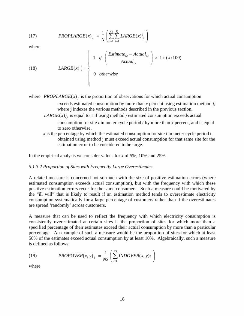
x is the percentage by which the estimated consumption for site i in meter cycle period t obtained using method j must exceed actual consumption for that same site for the estimation error to be considered to be large.

In the empirical analysis we consider values for x of 5%, 10% and 25%. 5.1.3.2 Proportion of Sites with Frequently Large Overestimates A related measure is concerned not so much with the size of positive estimation errors (where estimated consumption exceeds actual consumption), but with the frequency with which these positive estimation errors recur for the same consumers. Such a measure could be motivated by the “ill will” that is likely to result if an estimation method tends to overestimate electricity consumption systematically for a large percentage of customers rather than if the overestimates are spread ‘randomly’ across customers. A measure that can be used to reflect the frequency with which electricity consumption is consistently overestimated at certain sites is the proportion of sites for which more than a specified percentage of their estimates exceed their actual consumption by more than a particular percentage. An example of such a measure would be the proportion of sites for which at least 50% of the estimates exceed actual consumption by at least 10%. Algebraically, such a measure is defined as follows:

(19) ⎟⎠

⎞⎜⎝

⎛= ∑

=

NS

i

jij yxINDOVER

NSyxPROPOVER

1),(1),(

where

18

(20) ⎪⎩

⎪⎨⎧ >

=otherwise

yxOVERifyxINDOVER

ji

ji

0

100/)(1),(

(21) ∑=

=iT

t

jti

i

ji LARGEx

TxOVER

1,

1)(

and is the proportion of sites for which estimated consumption exceeds

actual consumption by more than x percent for more than y percent of the metering cycles using estimation method j, where j indexes the various methods described in the previous section,

jyxPROPOVER ),(

jiyxINDOVER ),( is an index that is equal to 1 if, using method j, estimated consumption

exceeds actual consumption for site i by more than x percent for more than y percent of the meter cycles for which estimates are made.

jixOVER )( is the proportion (0 < < 1) of estimates for site i using method j for

which estimated consumption exceeds actual consumption by more than x percent,

jixOVER )(

x is the percentage by which the estimated consumption for site i in meter cycle period t must exceed actual consumption for that same site for the estimation error to be considered to be large.

y is the percentage of estimates for each site that must involve overestimates of x percent or more for that same site to be considered as being frequently overestimated.

In the empirical analysis we consider values for x of 5%, 10% and 25%, and values of y of 50%, 60%, 67%, and 75%. Thus, for example, would indicate the proportion of sites for which at least 60% of estimates obtained using method j exceed actual consumption by 10% or more. We only apply this measure to sites for which there are estimates for at least one year.

jPROPOVER )60,10(

5.2 Aggregate Results: The five estimation methods were applied, wherever applicable, to the full sample of Residential, Small Commercial, and Medium Commercial sites. However, due to the need to construct electricity consumption histories for each site, the total number of data points (N) used varies with each method. For each method the all applicable data points are used, although for comparison purposes each method is also applied using the subset of data points that can be applied to all methods. First we consider the performance of the five estimation methods considered in terms of AEE and RMSPE. The results using these evaluation criteria are presented in Tables 1a, 1b, and 1c. The first three columns of these tables provide results using all available data points for each of the respective estimation methods, while the last three columns provide summary statistics for

19

the group of observations for which there is sufficient data for all estimation methods to be applied. While Method A appears to be unambiguously preferred for Residential sites, the results are mixed for Commercial sites. 5.2.1 Residential: For Residential customers, Method A (the method currently used by EDI) always performs the best according to both standard statistical evaluation measures and using both comparison groups. The AEE measure of the average difference of the estimate from actual consumption indicates a very small tendency for Method A to overestimate, while Method B and Method C (which are the next best in terms of both average difference and RMSPE) both tend to underestimate by amounts that are 10 times larger in absolute value. The remaining two methods exhibit much larger average overestimates, and perform worst in terms of RMSPE. The RMSPE values indicate that the methods based on the previous metering period’s information perform better than those based on a similar period from the previous year. By far the worst estimation method, according to both measures, is Method E which is based partially on projections of energy consumption for the entire upcoming year, opening up greater possibilities for error. 5.2.2 Small Commercial: The results for Small Commercial sites are less clearcut than for Residential sites, although Method E always performs worst. No single method has the best performance. According to the AEE measure, Method B outperforms the other estimation strategies by a wide margin. Thus, according to the AEE criterion, basing the estimate purely on site-specific consumption in the preceding period is better than applying the customer’s previous share of NSL to the current value of NSL. Method B tends to underestimate actual consumption, with the absolute value of the underestimate being approximately 5 times smaller than the overestimate from Method A. In terms of the RMSPE criterion, Method A performs best when each method is evaluated using all observations for which that method can be applied. However, when the evaluation is based on the subset of observations for which all methods can be applied, Method C and Method D have the smallest RMSPE. Thus, for this subset of observations, estimation methods that take account of energy consumption patterns from the same general period of time in the previous year (without projecting annual consumption) perform the best. Even so, Method A is not outperformed by much, as its RMSPE value is similar in magnitude to those for Method C and Method D. 5.2.3 Medium Commercial: As was the case for Small Commercial sites, Method B proves to be more accurate than the other methods in terms of the average difference between estimated and actual consumption (AEE). This is especially evident for the subset of observations for which all estimation methods can be applied, where the absolute values of the average errors for the other methods are all more than 100 times the value for Method B.

20

Depending on the set of observations being considered, Method A ranges from having the best RMSPE to the worst, although the RMSPE measures tend to be reasonably similar for all methods. Based on the subset of observations for which all methods can be applied, Method A is best, followed by Method B which also uses information from the previous metering period. However, when the evaluation is based on all available observations for each method, the ranking of methods according to RMSPE is opposite, with the methods based on information from the previous year performing the best in terms of RMSPE (but the worst in terms of average forecast error). 5.3 Robustness of Aggregate Results It is only for Residential sites that a single method consistently outperforms the others for the aggregate data. To assess the robustness of this result, the analysis in the previous section was repeated on subsamples obtained by subdividing the residential sample into ten groups of approximately 50,000 meter-cycle observations. The AEE and RMSPE results for these various ten subsamples are presented in Tables 2a-2j. These results indicate that the ranking of the different methods is somewhat sensitive to the sample metering cycles examined. Method A always has the smallest average estimation error (AEE) when the methods are evaluated using all observations for which each can be applied, and is always ranked first or second by this criterion when considering only those observations for which all methods can be applied. However, the findings using RMSPE are not quite as robust. Using all observations for which each method can be applied, Method A has the smallest or second smallest RMSPE in 6 of the 10 subsamples, as is also the case with Method B, usually in the same subsamples. Method E has the smallest RMSPE using all observations for which it can be applied in 4 of the subsamples. When considering only those observations for which all methods can be applied, Method A has the smallest or second smallest RMSPE in 8 of the 10 subsamples, while the same result holds for Method B in 7 of these same 8 subsamples. 5.4 Patterns in Estimation Accuracy over Time: In addition to comparing the performance of the different estimation methods using the entire sample of data points, it is instructive to consider their performance in different time periods or seasons, since it may be the case that some methods perform better or worse than others in particular circumstances. To investigate this issue, both AEE and RMSPE were calculated separately for each year of the sample (2001, 2002, and 2003), as well as for each month of the year (using all three years combined), where the year and month refers to the date at the midpoint of each meter reading cycle. These values are presented in Tables 3a-3f for the various estimation methods and customer types. Except for 2001, during which time there are sufficient data points to calculate estimates only for Methods A and B, the measures in each case are calculated using the subset of data points for which all estimation methods can be applied. Thus,

21

the relevant comparisons that can be made are between the values in Tables 3a-3f and those in the final three columns of Tables 1a-1c, although the actual subset of observations used is not the same in the different tables. 5.4.1 Residential: Although the average estimation error (AEE) is smallest for Method A in every year, this method does not provide the most accurate estimates for any particular month (season), as it is always outperformed by one or more of the other methods. It is only when averaged over the entire year (or sample) that Method A performs well. In fact, both methods (Method A and Method B) that are based on information on consumption in the previous meter-reading period tend to overestimate over the period from February through July, and underestimate over the period from August through January. Of the methods that make use of information on actual consumption from the previous year, Methods D and E tend to overestimate for every year and in every season, while Method C has a strong tendency to underestimate consumption. With respect to RMSPE (Table 3a), when results are broken down by year or season, Method A is often (although not always) outperformed by Method B, and infrequently by the other methods that use information from consumption behaviour in the previous year. It is only when averaged across all years or seasons that the performance of Method A is ranked the highest (or second highest after Method B) of the various methods examined. 5.4.2 Small Commercial: When averaged over all years and seasons (Table 1b), Method B is clearly more accurate in terms of average estimation error, while all but Method E have fairly similar RMSPE values (with Method C being the most accurate according to this measure). However, as was the case with the Residential sector, the aggregate results do not always hold across time or across seasons. While Method B has the smallest average error in every year (Table 3d), in most seasons, it is outperformed by Method C or Method D. Thus, in any particular season, a method that looks at the previous year’s consumption for that site performs better in terms of having a smaller AEE value. Method A is found to exhibit behaviour that is similar to that observed for the Residential sites, except in this case it tends to overestimate, on average, for September through January, and underestimate for the remaining months. From year to year, no single estimation method consistently performs best in terms of the RMSPE criterion (Table 3c), with the methods using information from the previous period performing better in 2003 but worse in 2002 than methods that use information from the previous year, although Method E has the smallest RMSPE of all methods in 2003. In terms of RMSPE in different months, Methods A and B which only consider consumption in the previous metering period perform better in most months, although one of the other three methods outperforms these in April, May and July.

22

5.4.3 Medium Commercial: For the Medium Commercial sites, meter readings generally occur on a monthly basis, so that there are a sufficient number of observations to include 2004 in Tables 3e and 3f. In 2002 and 2003, Method B, which performed best overall with respect to average estimation error (Table 1c), performs best on an annual basis, although Method E does better in the limited set of observations available for 2004. Method B occasionally performs best in terms of smallest AEE on a seasonal basis, although Method A is best in two months while Method C is best in five months and Method E is the best in January and November. Interestingly, we again observe that Method A exhibits a distinct pattern of overestimation and underestimation, with overestimates occurring from July through December, and underestimates in the remaining six months. As with the other types of sites, RMSPE rankings vary across years and seasons, although Method A performs at least as well as other methods in the majority of months and in some years. 5.5 Proportion of Large Consumption Overestimates As noted in Section 5 apart from standard statistical evaluation methods, such as AEE and RMSPE, the effectiveness of particular estimation methods can also be assessed in terms of the extent or frequency of the over- and under-estimates that are made. Specifically, as defined in Section 5.1.3.1, we calculate , the proportion of observations for which estimated consumption exceeds actual consumption by more than a specified percentage (x) using each estimation method. The specified percentages that are used in the calculations here are x = 5%, 10% and 25%. For each value of x, is calculated for all three types of customers. All calculations are based on the subset of observations for which all estimation methods can be applied, except for 2001 where we examine all observations for which Methods A and B can be applied. These results are presented in Tables 4a-4f.

PROPLARGEx

PROPLARGEx

5.5.1 Residential Customers Table 4a shows that for residential customers, the lowest rate of substantial overestimates in any given year occurs using Method A. This method always performs best in terms of having the smallest proportion of estimates that exceed actual values by more than 10% or by more than 25%. Even so, approximately 10% of all estimates are over by more than 25%, even for the best performing method. In general, the methods based on information from the previous year perform worse than those based on the previous metering period when it comes to the proportion of large overestimates of electricity use. The superior performance of Method A continues to hold up in general when we examine proportions of overestimates by time of year (Table 4b). For 7 of the 12 months, Method A ranks best in terms of having the smallest proportion of large (>25%) overestimates, and only

23

twice is it outside of the top 2 in this category. In both cases where Method A is 3rd best, it has rates of large overestimation that are very similar to the methods that outperform it. There are distinct seasonal patterns for Method A. While generally the proportion of large (>25%) overestimates is at or below 0.09, this proportion is higher for April through July with values in the 0.11 to 0.17 range. 5.5.2 Small Commercial Customers Tables 4c and 4d contain the results for small commercial customers. Proportions of large (>25%) overestimates are more similar across estimation methods than for residential customers, with proportions generally exceeding 0.15. There is no method that is unambiguously preferable in terms of this particular evaluation criterion. Furthermore, methods based on information from the previous year tend to do as well as those based on the previous metering period. Seasonal patterns for Method A are also discernable for the small commercial customers, with the lowest proportions of large overestimates occurring in January through March, while the highest proportions occur during May, June, and July. 5.5.3 Medium Commercial Customers The results for Medium Commercial customers are presented in Tables 4e and 4f. On a year-by-year basis, Method A tends to do quite well in terms of the proportion of large overestimates, although there is often not much difference in comparison to Method B. Large overestimates occur for only 5 to 6% of the observations. Methods C and D tend to perform worst, with 7% to 13% of the estimates generated via these methods involving substantial overestimates. During some times of year Methods A and B outperform the methods based on information from the previous year by wide margins. This tends to occur in the January through March period where only 1% to 2% of estimates obtained using these two methods exceed actual consumption by more than 25%. It is more difficult to discern seasonal patterns in the proportion of large overestimates for these customers (who tend to have monthly meter readings anyway). 5.6 Proportion of Sites with Frequently Large Overestimates For each category of customers (residential, small commercial, and medium commercial), we calculate the percentage of customers for whom more than 75%, 67%, 60%, or 50% of consumption estimates exceed actual consumption. This is repeated for estimates that exceed actual consumption by at least 5%, 10% and 25%. Only sites for which there are at least one full year’s worth of meter-reading cycles are included. In addition, we limit our comparison to the set of observations for which all estimation methods can be applied. The results are reported in Tables 5a-5c. For almost all estimation methods and customer groups, a site is more likely to experience overestimates than underestimates. The only

24

exceptions are Method C for Medium Commercial customers and Method B for Residential customers. Some methods do much better than others in terms of the proportion of customers who are subjected to an ‘inordinate’ number of overestimates. For example, with residential sites, Method C would result in over 10% of the sites receiving overestimates more than 75% of the time. This is the case for fewer than 2% of the sites using Method A, and for fewer than 1% using Method B. In general, methods using information from the previous metering cycle tend to perform better in terms of having a smaller ‘inordinate’ numbers of overestimates than those based on information from the same general time span during the previous year. Method E, however, does tend to perform in a manner that is comparable to Methods A and B according to this metric. These results hold over all customer types. As the size of the overestimate that is considered increases, the same general patterns are observed across estimation methods. Overall, Method A appears to perform relatively well according to these criteria.

25

6. Proxied adjustments for weather and other seasonal factors

It is apparent, at least for Method A, that there are seasonal patterns associated with tendencies to over/underestimate electricity consumption. In this section we report on a limited examination of the suitability of using NSL per day as a proxy for capturing factors such as hours of daylight and temperature in the estimation of Residential electricity usage. Variations in daylight and temperature are expected to affect the demand for lighting and heating. This will affect aggregate demand and manifest itself, along with other factors, in variations in NSL. We assume that there is some ‘base’ proportion (α) of energy use that is unaffected by fluctuations in seasonal factors, while remaining energy use is sensitive to temperature, hours of daylight, etc. A straightforward approach (that does not require the matching-up of weather data with the varying start dates and lengths of the periods involved) to proxy the weather/environmental factors that affect demand is to factor in relative NSL data from the current and previous periods. (This is similar to the method used by ATCO that uses degree day information. ATCO uses 0 .772 for the ‘base load’ component and 0.228 for the ‘heat load’ percentage weights).8 Our “weather-adjusted” estimates are calculated as (22) EstimateWAit = α*Estimateit + (1- α)(NSLPDt/NSLPDt-1)*Estimateit where NSLPDt = net system load per day corresponding to the relevant time period; For Methods A and B, t-1 is the immediately preceding period. For the remaining methods, t-1 refers to the same ‘period’ in the previous year. Since α is not known, we estimate it for early periods in the sample, and apply this estimate to later periods. The basic methodology we follow is: (i) Use ‘early’ (observations with start dates up to and including December 2002) data to estimate α by finding the value that minimizes (23) Σ(Consit-EstimateWAit)2

- For Method A and Method C these yield values in the acceptable range of 0 to 1. The value obtained for Method A is also applied to Method B. The value obtained for Method C is also applied to Method D.

(ii) the values obtained in (i) are applied to estimates for the later period (observations with start dates during or after January 2003)

8 As specified in the ENMAX document “Reasonability of Estimation Approaches for Settlement and Billing”, dated August 31, 2004.

26

The results for these ‘weather-adjusted’ estimation methods appear in Table 6. In general, using a proxied ‘weather-adjustment’ does not lead to much improvement in performance. For Method A, although the adjustment leads to an improvement in RMSPE, there is a deterioration in the magnitude of the average difference between estimated and actual consumption when compared to the unadjusted estimates over the same set of observations. For Method B, the estimates improve according to both of our measures, with the improvement in the average estimating error being large enough to make its performance better than that of Method A. According to the RMSPE measure, Method A is still preferred over all of the other methods after the weather adjustments. The remaining methods perform less well after the proxied weather adjustment. This may be due to a variety of factors including a limited ability of NSL to proxy accurately for weather-related factors (especially since the number of sites is steadily increasing) and possible shifts over time of the proportion of electricity usage that is sensitive to temperature or hours of daylight. In further work it may be possible to improve upon these ‘weather-adjusted’ estimates by directly matching observed weather data (such as cooling degree days) with the meter-reading intervals.

27

7. Summary and Conclusions

We have examined several estimation methodologies that utilize electricity consumption information from previous periods, as well as – in some cases – additional information such as proxies for weather-related variables. These methodologies have been used to estimate electricity consumption over metering cycles for a random sample of residential, small commercial, and medium commercial sites in Edmonton, over a time span of approximately three and a half years. Furthermore, these methods have been evaluated according to a series of metrics ranging from standard statistical criteria such as average estimation error (AEE) and root mean square percentage error (RMSPE) to measures designed to capture potential customer ‘disenchantment’ that are based on the percentage of overestimates of various magnitudes. These evaluation criteria are examined in aggregate, by year, by time of year, and for the final criterion, by site. Our findings indicate that no single estimation method performs best in all circumstances or according to all criteria. On aggregate, the current method used by EDI, which employs information from the immediately preceding metering cycle, performs best for residential sites and also performs well for small commercial sites. It does not fare as well for medium commercial sites, for which the number of observations available for analysis is much smaller. An alternative method, based as well on information from the immediately preceding metering cycle, also performs well with the aggregate data, and in some cases does better than or as well as the EDI method. However, particularly for small and medium commercial sites, estimation methods that utilize information on the electricity consumption history for the site from the same period in the previous year perform better according to some of the selected evaluation criteria. Our analysis also indicates that the relative performance of the various estimation methodologies is somewhat sensitive to the sample of observations selected. Nevertheless, for residential sites, the two methods that utilize consumption history from the immediately preceding meter cycle generally perform the best. In terms of performance in different years or months, no single estimation method does well in all cases. For residential sites, the EDI method performs well regardless of the particular year, but not in all months, and is frequently outperformed by an alternative method that relies on information from the previous meter cycle. Interestingly, both of these methods exhibit strong seasonal patterns, tending to overestimate in some months and underestimate in others. This suggests that the performance of these methods may be enhanced by including additional seasonal information. For residential sites the EDI method has the lowest rate of substantial overestimates of all estimation methods considered, although approximately 10% of all estimates exceed actual values by more than 25%, even for the best performing method. In general, for all types of sites, methods that utilize information from the previous meter cycle tend to yield better estimates according to this criterion than those utilizing information from the same period in the previous year. These same two methods also tend to result in smaller proportions of sites that receive overestimates in a large proportion of cases. Future work of interest to firms who must invoice for electricity use in the absence of meter readings could involve the evaluation of the potential benefits that might accrue from the

28

incorporation of supplemental information on weather such as cooling and heating degree days over the estimation period into the various methods considered.

29

References

“Appendix A: Estimation Methodology & Validation Thresholds” Baraniecki, J.M. and S. Koehn (2002), “Proposed Billing Estimation Method Using

Consumption Profiles”, Working Paper, EPCOR Energy Services Inc, November. ENMAX Corporation (2004), “Reasonability of Estimation Approaches for Settlement and

Billing”, mimeo, August.

30

Table 1a: Aggregate Results – Residential (26,990 sites) Based on all observations for which

individual Estimation Method can be applied.

Based on subset of observations for which all Estimation Methods can be applied (N=199053)

Average Difference between Estimated and Actual Consumption

Root Mean Square Percentage Error

Average Consumption

Average Difference between Estimated and Actual Consumption

Root Mean Square Percentage Error

Average Consumption

Method A 0.658 (N=460287)

6.510 1005.84 0.866 5.738 1042.09

Method B -9.012 (N=460287)

6.662 1005.84 -10.345 6.104 1042.09

Method C -10.682 (N=227356)

7.670 1045.56 -2.830 7.619 1042.09

Method D 30.400 (N=227356)

7.816 1045.56 33.136 7.772 1042.09

Method E 79.514 (N=199059)

9.842 1042.12 79.530 9.842 1042.09

Table 1b: Aggregate Results – Small Commercial (2,696 sites) Based on all observations for which

individual Estimation Method can be applied.

Based on subset of observations for which all Estimation Methods can be applied (N= 11395)

Average Difference between Estimated and Actual Consumption

Root Mean Square Percentage Error

Average Consumption

Average Difference between Estimated and Actual Consumption

Root Mean Square Percentage Error

Average Consumption

Method A 28.37 (N=57089)

20.23 3738.95 34.88 24.88 3141.81

Method B -4.82 (N=57089)

20.77 3738.95 -7.39 27.58 3141.81

Method C -46.49 (N=13408)

22.94 3135.70 -33.63 23.17 3141.81

Method D 76.39 (N=13408)

23.95 3135.70 74.37 24.32 3141.81

Method E 3166.34 (N=11396)

203.67 3142.51 3167.05 203.67 3141.81

31

Table 1c: Aggregate Results – Medium Commercial (300 sites) Based on all observations for which

individual Estimation Method can be applied.

Based on subset of observations for which all Estimation Methods can be applied (N= 5224)

Average Difference between Estimated and Actual Consumption

Root Mean Square Percentage Error

Average Consumption

Average Difference between Estimated and Actual Consumption

Root Mean Square Percentage Error

Average Consumption

Method A 107.23 (N=9480)

3.58 21022.47 108.91 1.85 21517.03

Method B -33.85 (N=9480)

3.56 21022.47 1.06 1.89 21517.03

Method C -131.01 (N=5686)

1.95 21397.88 -162.47 2.03 21517.03

Method D 726.51 (N=5686)

2.03 21397.88 664.02 2.11 21517.03

Method E 208.95 (N=5238)

2.22 21501.75 206.83 2.23 21517.03

32

Table 2a: Aggregate Results –Residential Sub-Sample #1 (2,632 sites) Based on all observations for which

individual Estimation Method can be applied.

Based on subset of observations for which all Estimation Methods can be applied (N=20284)

Average Difference between Estimated and Actual Consumption

Root Mean Square Percentage Error

Average Consumption

Average Difference between Estimated and Actual Consumption

Root Mean Square Percentage Error

Average Consumption

Method A 1.808 (N=46844)

4.270 1019.31 1.544 1.488 1046.96

Method B -7.512 (N=46844)

4.670 1019.31 -9.060 1.641 1046.96

Method C -5.382 (N=23137)

2.709 1051.93 2.298 2.742 1046.96

Method D 36.503 (N=23137)

2.863 1051.93 38.680 2.867 1046.96

Method E 33.469 (N=20284)

0.766 1046.96 33.469 0.766 1046.96

Table 2b: Aggregate Results –Residential Sub-Sample #2 (2,630 sites) Based on all observations for which

individual Estimation Method can be applied.

Based on subset of observations for which all Estimation Methods can be applied (N=20478)

Average Difference between Estimated and Actual Consumption

Root Mean Square Percentage Error

Average Consumption

Average Difference between Estimated and Actual Consumption

Root Mean Square Percentage Error

Average Consumption

Method A 2.034 (N=46779)

3.598 1000.04 2.632 2.400 1030.11

Method B -7.182 (N=46779)

3.517 1000.04 -7.230 2.328 1030.11

Method C -6.337 (N=23371)

3.265 1035.12 1.082 3.359 1030.11

Method D 35.076 (N=23371)

3.426 1035.12 37.126 3.531 1030.11

Method E 52.003 (N=20479)

2.775 1030.15 52.017 2.775 1030.11

33

Table 2c: Aggregate Results –Residential Sub-Sample #3 (2,627 sites) Based on all observations for which

individual Estimation Method can be applied.

Based on subset of observations for which all Estimation Methods can be applied (N=20471)

Average Difference between Estimated and Actual Consumption

Root Mean Square Percentage Error

Average Consumption

Average Difference between Estimated and Actual Consumption

Root Mean Square Percentage Error

Average Consumption

Method A 1.809 (N=46758)

11.410 1009.26 0.845 1.705 1035.14

Method B -7.607 (N=46758)

11.729 1009.26 -10.077 1.734 1035.14

Method C -7.324 (N=23308)

12.178 1038.82 -1.851 10.664 1035.14

Method D 34.038 (N=23308)

12.545 1038.82 34.122 11.123 1035.14

Method E 39.114 (N=20471)

3.158 1035.14 39.114 3.158 1035.14

Table 2d: Aggregate Results –Residential Sub-Sample #4 (2,618 sites) Based on all observations for which

individual Estimation Method can be applied.

Based on subset of observations for which all Estimation Methods can be applied (N=20257)

Average Difference between Estimated and Actual Consumption

Root Mean Square Percentage Error

Average Consumption

Average Difference between Estimated and Actual Consumption

Root Mean Square Percentage Error

Average Consumption

Method A 3.125 (N=46715)

3.436 1018.97 0.721 2.283 1054.68

Method B -6.606 (N=46715)

3.277 1018.97 -10.420 2.105 1054.68

Method C -6.756 (N=23068)

3.397 1057.51 -1.812 3.260 1054.68

Method D 35.354 (N=23068)

3.482 1057.51 34.907 3.333 1054.68

Method E 36.767 (N=20258)

2.649 1054.71 36.781 2.649 1054.68

34

Table 2e: Aggregate Results –Residential Sub-Sample #5 (2,619 sites) Based on all observations for which

individual Estimation Method can be applied.

Based on subset of observations for which all Estimation Methods can be applied (N=20462)

Average Difference between Estimated and Actual Consumption

Root Mean Square Percentage Error

Average Consumption

Average Difference between Estimated and Actual Consumption

Root Mean Square Percentage Error

Average Consumption

Method A 1.577 (N=46793)

2.952 1003.36 0.961 3.775 1034.25

Method B -7.706 (N=46793)

2.816 1003.36 -10.020 3.510 1034.25

Method C -6.641 (N=23335)

3.563 1039.64 -0.161 3.801 1034.25

Method D 34.694 (N=23335)

3.629 1039.64 35.840 3.870 1034.25

Method E 31.956 (N=20462)

8.829 1034.25 31.956 8.829 1034.25

Table 2f: Aggregate Results –Residential Sub-Sample #6 (2,623 sites) Based on all observations for which

individual Estimation Method can be applied.

Based on subset of observations for which all Estimation Methods can be applied (N=20081)

Average Difference between Estimated and Actual Consumption

Root Mean Square Percentage Error

Average Consumption

Average Difference between Estimated and Actual Consumption

Root Mean Square Percentage Error

Average Consumption

Method A 2.146 (N=46806)

7.873 1009.34 2.008 11.489 1038.83

Method B -7.027 (N=46806)

8.284 1009.34 -8.935 12.089 1038.83

Method C -7.264 (N=23067)

10.161 1043.98 -0.146 10.861 1038.83

Method D 34.407 (N=23067)

10.381 1043.98 36.124 11.096

1038.83

Method E 52.595 (N=20182)

23.369 1038.85 52.605 23.370 1038.83

35

Table 2g: Aggregate Results –Residential Sub-Sample #7 (2,623 sites)

Based on all observations for which individual Estimation Method can be applied.

Based on subset of observations for which all Estimation Methods can be applied (N=20301)

Average Difference between Estimated and Actual Consumption

Root Mean Square Percentage Error

Average Consumption

Average Difference between Estimated and Actual Consumption

Root Mean Square Percentage Error

Average Consumption

Method A 2.014 (N=46785)

7.937 1011.70 1.404 11.851 1050.92

Method B -7.357 (N=46785)

8.789 1011.70 -9.619 13.155 1050.92

Method C -7.862 (N=23142)

10.334 1055.47 0.094 11.023 1050.92

Method D 34.006 (N=23142)

10.438 1055.47 36.545 11.131

1050.92

Method E 46.357 (N=20301)

11.341 1050.92 46.357 11.341 1050.92

Table 2h: Aggregate Results –Residential Sub-Sample #8 (2,625 sites) Based on all observations for which

individual Estimation Method can be applied.

Based on subset of observations for which all Estimation Methods can be applied (N=20689)

Average Difference between Estimated and Actual Consumption

Root Mean Square Percentage Error

Average Consumption

Average Difference between Estimated and Actual Consumption

Root Mean Square Percentage Error

Average Consumption

Method A 2.245 (N=46852)

2.736 1012.13 1.040 3.049 1055.05

Method B -7.035 (N=46852)

2.622 1012.13 -9.828 2.813 1055.05

Method C -4.523 (N=23527)

8.339 1058.08 2.585 8.134 1055.05

Method D 37.584 (N=23527)

8.571 1058.08 39.155 8.412 1055.05

Method E 44.492 (N=20689)

3.372 1055.05 44.492 3.372 1055.05

36

Table 2i: Aggregate Results –Residential Sub-Sample #9 (2,624 sites)

Based on all observations for which individual Estimation Method can be applied.

Based on subset of observations for which all Estimation Methods can be applied (N=20545)

Average Difference between Estimated and Actual Consumption

Root Mean Square Percentage Error

Average Consumption

Average Difference between Estimated and Actual Consumption

Root Mean Square Percentage Error

Average Consumption

Method A 2.121 (N=46721)

5.740 1016.99 2.383 3.087 1055.98

Method B -7.323 (N=46721)

5.626 1016.99 -8.392 3.107 1055.98

Method C -7.461 (N=23389)

9.390 1058.36 0.281 9.346 1055.98

Method D 34.403 (N=23389)

9.308 1058.36 36.816 9.175 1055.98

Method E 176.593 (N=20546)

10.866 1055.99 176.567 10.866 1055.98

Table 2j: Aggregate Results –Residential Sub-Sample #10 (3,369 sites) Based on all observations for which

individual Estimation Method can be applied.

Based on subset of observations for which all Estimation Methods can be applied (N=15385)

Average Difference between Estimated and Actual Consumption

Root Mean Square Percentage Error

Average Consumption

Average Difference between Estimated and Actual Consumption

Root Mean Square Percentage Error

Average Consumption

Method A -14.787 (N=39234)

9.072 948.04 -6.754 1.409 1011.41

Method B -27.796 (N=39234)

8.589 948.04 -22.990 1.247 1011.41

Method C -57.969 (N=18012)

4.618 1008.36 -39.932 4.568 1011.41

Method D -24.473 (N=18012)

4.760 1008.36 -8.154 4.724 1011.41

Method E 346.614 (N=15387)

7.550 1011.60 346.841 7.550 1011.41

37

Table 3a: Variations in RMSPE over Time – Residential

Number of Observations

Method A Method B Method C Method D Method E

Year 2001 139263 8.41 8.36 n.a. n.a. n.a. 2002 90665 2.40 2.30 6.51 6.80 7.42 2003 108381 7.46 8.00 8.44 8.50 11.48 Month January 18633 3.56 3.24 11.38 11.92 3.36 February 8586 0.39 0.38 1.88 1.98 0.61 March 9727 3.56 3.77 10.44 10.59 3.38 April 15863 4.54 5.28 2.94 2.95 2.77 May 18825 10.95 12.38 10.81 10.89 10.58 June 17804 11.93 12.66 10.58 10.28 6.21 July 17652 1.76 1.70 4.17 4.29 4.88 August 18302 2.95 2.86 4.82 5.07 11.55 September 18639 1.02 1.01 3.44 3.58 2.44 October 18307 3.57 3.53 7.29 7.38 5.77 November 18637 1.90 1.71 6.65 6.89 3.61 December 18078 5.46 4.69 7.42 7.73 26.00

Table 3b: Variations in Average Estimation Error over Time – Residential

Actual Consumption

Method A Method B Method C Method D Method E

Year 2001 997.34 -6.73 -24.72 n.a. n.a. n.a. 2002 1027.89 -2.49 -16.48 -15.26 36.59 109.35 2003 1054.01 3.64 -5.24 7.55 30.24 54.55 Month January 1321.15 -28.91 -121.71 -13.39 38.27 47.50 February 1157.55 31.73 13.66 -1.69 41.88 -6.09 March 1115.33 50.64 133.73 29.82 39.71 103.62 April 952.24 29.41 159.86 -8.04 24.12 49.18 May 931.62 41.80 176.31 -17.90 20.30 39.18 June 897.22 55.44 95.20 -5.62 29.01 73.51 July 965.32 35.22 1.11 -14.09 30.42 91.71 August 944.99 -8.79 -25.57 -8.22 27.46 197.58 September 967.48 -28.14 -22.15 -0.039 24.58 108.84 October 986.51 -35.31 -82.73 7.76 39.73 82.58 November 1105.14 -43.12 -165.20 1.07 38.06 71.58 December 1238.27 -43.19 -182.81 11.78 50.95 58.30

38

Table 3c: Variations in RMSPE over Time – Small Commercial

Number of observations

Method A Method B Method C Method D Method E

Year 2001 17037 21.53 21.94 n.a. n.a. n.a. 2002 5119 30.40 34.18 17.82 18.66 303.74 2003 6275 19.25 20.71 26.76 28.10 8.18 Month January 954 2.59 2.44 4.17 4.36 3.08 February 551 0.56 0.55 1.10 1.16 0.67 March 496 2.10 2.24 2.41 2.44 2.53 April 941 14.73 17.02 21.11 22.49 5.27 May 1073 72.59 82.18 2.88 3.02 3.37 June 1082 16.04 17.13 18.30 20.07 17.18 July 928 28.50 27.38 3.95 4.08 80.58 August 1136 2.11 2.17 41.81 43.73 17.37 September 960 0.48 0.48 2.52 2.56 1.91 October 1156 0.63 0.60 1.69 1.74 5.99 November 942 1.13 1.00 1.59 1.64 3.53 December 1176 11.30 10.13 52.94 55.28 629.43

Table 3d: Variations in Average Estimation Error over Time – Small Commercial

Actual Consumption

Method A Method B Method C Method D Method E

Year 2001 3769.20 48.87 -11.17 n.a. n.a. n.a. 2002 3076.54 40.35 -5.42 -41.37 118.13 6291.29 2003 3195.14 30.45 -8.96 -27.21 38.78 618.42 Month January 3248.59 97.98 -142.01 18.23 149.34 300.18 February 3454.36 -68.24 -77.36 -84.57 34.72 46.63 March 2946.77 -144.74 51.03 55.53 83.67 60.58 April 3071.82 -105.83 290.49 -111.05 -21.80 219.75 May 2720.11 -139.64 216.90 -0.38 126.25 250.69 June 3337.81 -271.58 -167.98 -114.03 2.87 195.08 July 3060.66 -99.60 -200.55 10.07 155.16 33346.54 August 3380.81 -4.71 -70.09 -118.38 2.10 1344.21 September 2838.85 175.53 195.58 64.52 138.39 267.82 October 3102.84 355.21 182.28 -71.57 21.79 423.13 November 2886.10 218.74 -135.77 47.28 145.90 256.34 December 3575.01 228.93 -221.57 -44.09 71.80 1359.95

39

Table 3e: Variations in RMSPE over Time – Medium Commercial

Number of observations

Method A Method B Method C Method D Method E

Year 2001 2798 2.33 2.21 n.a. n.a. n.a. 2002 2419 1.43 1.36 1.42 1.54 2.20 2003 2619 2.22 2.33 2.52 2.57 2.33 2004 185 0.14 0.14 0.57 0.60 0.25 Month January 412 0.31 0.31 0.55 0.58 0.38 February 396 0.11 0.11 0.31 0.33 0.15 March 427 0.28 0.29 0.51 0.54 0.36 April 445 0.21 0.25 2.08 2.29 4.10 May 445 5.36 5.63 6.03 6.17 5.57 June 437 0.20 0.20 1.47 1.63 0.49 July 436 0.22 0.21 0.74 0.79 0.21 August 436 0.21 0.23 0.64 0.66 0.47 September 425 0.33 0.33 0.91 0.91 0.31 October 478 0.27 0.25 0.59 0.60 0.24 November 451 3.27 3.11 1.63 1.69 3.02 December 436 0.16 0.14 0.50 0.53 0.23

Table 3f: Variations in Average Estimation Error over Time – Medium Commercial

Actual Consumption

Method A Method B Method C Method D Method E

Year 2001 20503.97 336.94 126.69 n.a. n.a. n.a. 2002 21413.85 200.46 78.45 -187.66 1051.95 191.05 2003 21515.68 129.43 32.88 -122.06 316.63 246.08 2004 22882.16 -1371.46 -1457.07 -397.61 514.19 -140.77 Month January 22643.50 -428.15 -955.71 -506.54 526.58 -310.97 February 22167.17 -632.36 3.04 -360.09 661.35 105.71 March 20988.52 -170.17 456.99 -343.48 882.69 181.75 April 20738.24 -712.15 1227.09 41.04 939.06 642.64 May 19599.93 -1035.34 -25.55 209.55 905.89 258.94 June 22296.04 -883.07 -1391.13 -104.61 736.48 249.34 July 22914.54 227.75 -680.77 -714.19 477.91 -382.31 August 22039.04 528.45 1061.83 -333.05 352.74 488.93 September 20523.15 699.14 768.77 24.07 443.70 466.98 October 20619.12 1038.27 -64.03 235.23 758.45 347.13 November 21260.37 779.24 -920.01 -176.79 585.07 -108.15 December 22649.56 1737.14 524.89 -6.69 672.27 497.42

40

Table 4a: Proportion of Overestimates by Year: Residential

Method A Method B Method C Method D Method E 2001-2004 (N=199053) over 0.50542 0.47618 0.48329 0.56947 0.51559 >5% over 0.36668 0.37640 0.36745 0.44656 0.38815 >10% over 0.25692 0.29169 0.28092 0.34120 0.28959 >25% over 0.10051 0.12865 0.14860 0.17313 0.13577 2001 (N=139263) over 0.49564 0.46516 n.a. n.a. n.a. >5% over 0.34527 0.35614 n.a. n.a. n.a. >10% over 0.23439 0.26524 n.a. n.a. n.a. >25% over 0.09053 0.10859 n.a. n.a. n.a. 2002 (N=90665) over 0.49523 0.45133 0.45708 0.58712 0.54505 >5% over 0.35871 0.35473 0.34393 0.46339 0.41598 >10% over 0.25185 0.27609 0.26189 0.35300 0.31166 >25% over 0.10042 0.12717 0.13777 0.17535 0.14559 2003 (N=108381) over 0.51392 0.49694 0.50521 0.55470 0.49093 >5% over 0.37332 0.39449 0.38712 0.43247 0.36485 >10% over 0.26112 0.30470 0.29681 0.33129 0.27110 >25% over 0.10053 0.12986 0.15763 0.17125 0.12754

41

Table 4b: Proportion of Overestimates by Time of Year: Residential

Method A Method B Method C Method D Method E January (N=18633) over 0.44421 0.22975 0.47389 0.57522 0.47459 >5% over 0.28026 0.13863 0.35421 0.44695 0.33747 >10% over 0.17662 0.09118 0.26802 0.33553 0.24054 >25% over 0.06183 0.04165 0.14142 0.16970 0.10760 February (N=8586) over 0.58805 0.53413 0.49849 0.58945 0.44025 >5% over 0.41847 0.37794 0.37584 0.46949 0.31249 >10% over 0.28302 0.25099 0.28360 0.35057 0.22502 >25% over 0.09050 0.08386 0.14826 0.17529 0.09318 March (N=9727) over 0.62702 0.81875 0.55289 0.57099 0.54806 >5% over 0.44741 0.69312 0.42397 0.44063 0.40896 >10% over 0.29392 0.53418 0.32867 0.34368 0.29053 >25% over 0.09551 0.17138 0.16850 0.17529 0.12841 April (N=15863) over 0.56818 0.86301 0.47412 0.55809 0.53653 >5% over 0.41247 0.77615 0.36639 0.43390 0.40100 >10% over 0.28986 0.64773 0.28242 0.33335 0.29685 >25% over 0.11208 0.28437 0.14903 0.17197 0.13572 May (N=18825) over 0.60223 0.86465 0.44356 0.55076 0.51384 >5% over 0.46502 0.78778 0.32961 0.42640 0.38444 >10% over 0.34194 0.68542 0.25131 0.32064 0.28382 >25% over 0.14215 0.34560 0.13344 0.16069 0.13163 June (N=17804) over 0.64081 0.73169 0.46950 0.55768 0.53173 >5% over 0.51696 0.61801 0.36217 0.45029 0.41446 >10% over 0.39794 0.49590 0.28280 0.35537 0.31931 >25% over 0.17350 0.23040 0.15783 0.18653 0.16069 July (N=17652) over 0.63494 0.53807 0.46142 0.57342 0.52736 >5% over 0.49405 0.39231 0.35027 0.45406 0.39837 >10% over 0.35883 0.27759 0.27034 0.35344 0.29532 >25% over 0.13709 0.10622 0.14486 0.17783 0.13732 August (N=18302) over 0.47323 0.40996 0.47071 0.55923 0.50535 >5% over 0.32193 0.26418 0.35799 0.44361 0.38504 >10% over 0.21167 0.17441 0.27576 0.34051 0.29439 >25% over 0.07786 0.06895 0.14878 0.17637 0.14392

…continued

42

Table 4b (continued) Proportion of Overestimates by Time of Year: Residential

Method A Method B Method C Method D Method E September (N=18639) over 0.37089 0.38854 0.48930 0.55416 0.53651 >5% over 0.25398 0.26589 0.37405 0.43157 0.41622 >10% over 0.17898 0.18762 0.28188 0.32459 0.31461 >25% over 0.07758 0.08058 0.15081 0.16589 0.15510 October (N=18307) over 0.37838 0.27312 0.49751 0.57961 0.53040 >5% over 0.27378 0.19801 0.37740 0.45261 0.40476 >10% over 0.19681 0.14781 0.28863 0.34397 0.31223 >25% over 0.09128 0.07238 0.14918 0.17414 0.15235 November (N=18637) over 0.41004 0.15995 0.49992 0.58556 0.50856 >5% over 0.29280 0.10967 0.37688 0.45737 0.38241 >10% over 0.19853 0.07673 0.28363 0.34609 0.28470 >25% over 0.07308 0.03724 0.14530 0.16972 0.12888 December (N=18078) over 0.44640 0.15134 0.50769 0.58978 0.51328 >5% over 0.30451 0.10084 0.39202 0.46073 0.38516 >10% over 0.19875 0.07080 0.29887 0.35358 0.28654 >25% over 0.07086 0.03701 0.15582 0.17740 0.12944

43

Table 4c: Proportion of Overestimates by Year: Small Commercial

Method A Method B Method C Method D Method E 2001-2004 (N=11395) over 0.52190 0.49829 0.50189 0.58008 0.51031 >5% over 0.42229 0.39017 0.37964 0.46327 0.38315 >10% over 0.33857 0.30838 0.30004 0.36218 0.29495 >25% over 0.17016 0.17376 0.16428 0.19158 0.16253 2001 (N=17037) over 0.53014 0.50420 n.a. n.a. n.a. >5% over 0.39473 0.35957 n.a. n.a. n.a. >10% over 0.28555 0.26484 n.a. n.a. n.a. >25% over 0.13101 0.12819 n.a. n.a. n.a. 2002 (N=5119) over 0.53292 0.50303 0.49873 0.61125 0.52080 >5% over 0.43602 0.39519 0.37878 0.49932 0.39715 >10% over 0.35085 0.31686 0.29635 0.39265 0.31237 >25% over 0.18031 0.18324 0.16175 0.20649 0.17347 2003 (N=6275) over 0.51299 0.49450 0.50454 0.55474 0.50167 >5% over 0.41116 0.38614 0.38040 0.43394 0.37163 >10% over 0.32861 0.30151 0.30311 0.33737 0.28064 >25% over 0.16191 0.16606 0.16637 0.17944 0.15347

44

Table 4d: Proportion of Overestimates by Time of Year: Small Commercial

Method A Method B Method C Method D Method E January (N=954) over 0.62264 0.39623 0.50524 0.61111 0.45912 >5% over 0.48218 0.22642 0.37841 0.48008 0.33543 >10% over 0.32600 0.14361 0.29874 0.36688 0.24423 >25% over 0.08386 0.04927 0.16771 0.19392 0.11740 February (N=551) over 0.41016 0.39564 0.48457 0.57895 0.43557 >5% over 0.27405 0.26860 0.34483 0.44102 0.31579 >10% over 0.21053 0.19056 0.26316 0.32486 0.22505 >25% over 0.08348 0.07986 0.15426 0.17241 0.11797 March (N=496) over 0.40726 0.59476 0.56048 0.58669 0.54637 >5% over 0.28226 0.44960 0.45968 0.46573 0.38105 >10% over 0.20968 0.32258 0.36895 0.39113 0.27419 >25% over 0.09879 0.15726 0.20565 0.21169 0.15524 April (N=941) over 0.43571 0.73326 0.46440 0.51647 0.51753 >5% over 0.34006 0.60043 0.36557 0.43677 0.39107 >10% over 0.28374 0.48247 0.29224 0.35069 0.28480 >25% over 0.15728 0.28587 0.16153 0.18385 0.14772 May (N=1073) over 0.44548 0.70270 0.49767 0.58900 0.48742 >5% over 0.37558 0.61044 0.37372 0.48555 0.36160 >10% over 0.32060 0.51445 0.30289 0.38397 0.27679 >25% over 0.19478 0.32246 0.16869 0.20317 0.14818 June (N=1082) over 0.51294 0.56100 0.46303 0.52773 0.49815 >5% over 0.43068 0.49076 0.35305 0.43068 0.38447 >10% over 0.36691 0.42237 0.29113 0.35397 0.30961 >25% over 0.22643 0.25970 0.16451 0.19593 0.18577 July (N=928) over 0.62392 0.56466 0.50647 0.58944 0.52047 >5% over 0.53017 0.46444 0.39009 0.49569 0.40841 >10% over 0.43750 0.34698 0.31358 0.40409 0.32220 >25% over 0.23491 0.19935 0.16379 0.20905 0.18103 August (N=1136) over 0.48680 0.42254 0.46743 0.55370 0.49384 >5% over 0.34595 0.29930 0.34947 0.43486 0.39085 >10% over 0.25528 0.23327 0.27641 0.33099 0.31690 >25% over 0.12852 0.12852 0.15317 0.17606 0.18574

….continued

45

Table 4d (continued): Proportion of Overestimates by Time of Year: Small Commercial

Method A Method B Method C Method D Method E September (N=960) over 0.47604 0.48646 0.52604 0.62292 0.54063 >5% over 0.37708 0.38229 0.40521 0.45417 0.41354 >10% over 0.30417 0.31563 0.33542 0.37083 0.32188 >25% over 0.15833 0.16875 0.18646 0.21563 0.17708 October (N=1156) over 0.53979 0.44983 0.50606 0.57699 0.55450 >5% over 0.46280 0.38235 0.37370 0.45242 0.39965 >10% over 0.39619 0.32699 0.27941 0.35208 0.31574 >25% over 0.24394 0.19810 0.14014 0.16263 0.17128 November (N=942) over 0.54034 0.33333 0.56688 0.63800 0.52442 >5% over 0.46921 0.26539 0.42463 0.52123 0.40764 >10% over 0.38004 0.21444 0.32484 0.39278 0.30892 >25% over 0.20382 0.12951 0.16667 0.20276 0.16136 December (N=1176) over 0.64626 0.36650 0.50595 0.58333 0.52636 >5% over 0.55102 0.23639 0.37415 0.46344 0.37840 >10% over 0.43793 0.15221 0.28486 0.33588 0.29252 >25% over 0.14626 0.06037 0.16156 0.18282 0.17007

46

Table 4e: Proportion of Overestimates by Year: Medium Commercial

Method A Method B Method C Method D Method E 2001-2004 (N= 5224) over 0.50766 0.49943 0.47473 0.60528 0.49904 >5% over 0.31585 0.29230 0.31145 0.43434 0.30475 >10% over 0.18817 0.17764 0.20463 0.28905 0.18224 >25% over 0.05532 0.05398 0.08078 0.10356 0.06011 2001 (N=2798) over 0.54753 0.52216 n.a. n.a. n.a. >5% over 0.33881 0.31523 n.a. n.a. n.a. >10% over 0.20944 0.18585 n.a. n.a. n.a. >25% over 0.07076 0.07005 n.a. n.a. n.a. 2002 (N=2419) over 0.52956 0.51509 0.47458 0.66887 0.50434 >5% over 0.33444 0.31087 0.32327 0.50351 0.31170 >10% over 0.20215 0.18768 0.21993 0.34808 0.18479 >25% over 0.06077 0.06160 0.08847 0.12774 0.06284 2003 (N=2619) over 0.50630 0.50630 0.47614 0.54868 0.49561 >5% over 0.31615 0.29133 0.30279 0.37113 0.30661 >10% over 0.18633 0.17946 0.19359 0.23597 0.18671 >25% over 0.05384 0.05040 0.07446 0.08247 0.05995 2004 (N=185) over 0.24324 0.20000 0.45946 0.57838 0.48108 >5% over 0.07027 0.06486 0.28108 0.42703 0.18919 >10% over 0.03243 0.02162 0.16216 0.27027 0.08649 >25% over 0.00541 0.00541 0.07027 0.08649 0.02703

47

Table 4f: Proportion of Overestimates by Time of Year: Medium Commercial

Method A Method B Method C Method D Method E January (N=412) over 0.41505 0.27913 0.45631 0.61893 0.46117 >5% over 0.20388 0.14563 0.26456 0.43204 0.22087 >10% over 0.11165 0.08010 0.16019 0.26214 0.12136 >25% over 0.01214 0.00971 0.06068 0.07767 0.02913 February (N=396) over 0.33333 0.56313 0.45202 0.62626 0.47980 >5% over 0.13384 0.21717 0.28535 0.44192 0.22727 >10% over 0.06313 0.09596 0.18182 0.27778 0.12374 >25% over 0.01263 0.01768 0.05303 0.07323 0.03283 March (N=427) over 0.41686 0.60656 0.47307 0.63466 0.47307 >5% over 0.16862 0.29040 0.29742 0.45667 0.29977 >10% over 0.08431 0.12412 0.16862 0.34426 0.16862 >25% over 0.02108 0.03513 0.06089 0.09836 0.05621 April (N=445) over 0.29213 0.70337 0.47191 0.62921 0.55281 >5% over 0.18427 0.43146 0.32135 0.45618 0.35281 >10% over 0.10787 0.29438 0.21348 0.31236 0.20000 >25% over 0.04045 0.07416 0.08764 0.12135 0.06966 May (N=445) over 0.29888 0.50787 0.48764 0.61798 0.53034 >5% over 0.17303 0.31236 0.33708 0.44270 0.31461 >10% over 0.10562 0.17303 0.24270 0.32135 0.19101 >25% over 0.04944 0.06742 0.10562 0.13258 0.07640 June (N=437) over 0.41648 0.35240 0.49199 0.60870 0.49886 >5% over 0.28146 0.21281 0.33410 0.45080 0.31350 >10% over 0.17391 0.15332 0.23570 0.29977 0.20137 >25% over 0.05492 0.05034 0.09840 0.13272 0.07780 July (N=436) over 0.50229 0.36468 0.39679 0.60780 0.42890 >5% over 0.30046 0.21789 0.27752 0.42202 0.29358 >10% over 0.19266 0.14450 0.18578 0.27523 0.18349 >25% over 0.09404 0.08028 0.07569 0.10550 0.06651 August (N=436) over 0.57798 0.66972 0.48624 0.56881 0.55275 >5% over 0.34633 0.46789 0.32110 0.43119 0.38761 >10% over 0.20413 0.27982 0.21789 0.27294 0.24771 >25% over 0.06193 0.07569 0.09862 0.11468 0.06422

…..continued

48

Table 4f (continued): Proportion of Overestimates by Time of Year: Medium Commercial

Method A Method B Method C Method D Method E September (N=425) over 0.64471 0.60471 0.48706 0.56706 0.54118 >5% over 0.42353 0.44000 0.30824 0.37882 0.33882 >10% over 0.29176 0.31294 0.20706 0.24706 0.20235 >25% over 0.07765 0.08471 0.08000 0.08941 0.07294 October (N=478) over 0.70293 0.48536 0.49791 0.59833 0.50628 >5% over 0.51464 0.30544 0.35146 0.42678 0.34100 >10% over 0.32636 0.19874 0.24477 0.28870 0.21548 >25% over 0.09414 0.06276 0.10042 0.11088 0.07741 November (N=451) over 0.63636 0.25721 0.48337 0.60532 0.44568 >5% over 0.42129 0.11530 0.30820 0.43681 0.24834 >10% over 0.21286 0.05987 0.18847 0.27273 0.15965 >25% over 0.04656 0.03104 0.07095 0.08426 0.04435 December (N=436) over 0.82110 0.60321 0.50688 0.58257 0.51376 >5% over 0.59862 0.34174 0.32110 0.43578 0.30505 >10% over 0.35780 0.20413 0.19954 0.29128 0.16055 >25% over 0.08945 0.05275 0.07110 0.09633 0.04816

49

Table 5a: Percentage of Sites with Frequent Overestimates – Residential

Percentage of estimates for each site that are overestimates more than 75% more than 67% more than 60% more than 50% over

Method A 1.69 9.17 23.70 55.68 Method B 0.94 5.62 15.14 44.66 Method C 12.52 23.17 33.79 50.03 Method D 22.60 36.03 48.24 64.24 Method E 2.41 10.58 25.61 58.43

at least 5% overestimate Method A 0.18 1.40 3.95 16.74 Method B 0.19 1.29 3.43 16.42 Method C 5.57 11.60 18.49 30.54 Method D 9.89 18.66 27.87 42.64 Method E 0.47 2.56 5.92 21.32

at least 10% overestimate Method A 0.06 0.31 0.79 4.72 Method B 0.04 0.40 0.92 6.01 Method C 2.98 6.71 11.06 19.93 Method D 4.85 9.99 15.75 26.43 Method E 0.20 0.94 1.89 8.37

at least 25% overestimate Method A 0.01 0.03 0.04 0.39 Method B 0.01 0.05 0.07 0.53 Method C 0.88 2.15 3.63 7.95 Method D 1.20 2.70 4.76 9.65 Method E 0.01 0.17 0.24 1.34

Note: Number of Sites =18031. Only sites with at least 6 estimates are included.

50

Table 5b: Percentage of Sites with Frequent Overestimates – Small Commercial

Percentage of estimates for each site that are overestimates more than 75% more than 67% more than 60% more than 50% over

Method A 2.19 10.07 26.22 58.72 Method B 1.00 8.28 20.14 50.75 Method C 16.55 25.32 36.39 52.84 Method D 25.92 38.48 49.05 64.51 Method E 1.69 9.97 24.73 56.43

at least 5% over Method A 0.50 2.79 5.98 27.62 Method B 0.20 2.09 5.28 18.44 Method C 8.18 14.56 20.94 32.80 Method D 13.16 20.94 29.41 43.87 Method E 0.50 2.49 6.28 23.03

at least 10% over Method A 0.30 1.00 2.09 11.76 Method B 0.00 0.90 1.79 8.47 Method C 5.18 8.87 13.76 23.33 Method D 7.08 12.96 18.74 29.81 Method E 0.40 1.00 2.79 11.37

at least 25% over Method A 0.00 0.30 0.30 2.09 Method B 0.00 0.30 0.40 2.89 Method C 1.50 2.69 4.09 9.47 Method D 1.99 3.89 11.57 11.57 Method E 0.00 0.50 0.90 3.49

Note: Number of Sites =1003. Only sites with at least 6 estimates are included.

51

Table 5c: Percentage of Sites with Frequent Overestimates – Medium Commercial

Percentage of estimates for each site that are overestimates more than 75% more than 67% more than 60% more than 50% over

Method A 0.86 3.00 13.73 58.37 Method B 0.43 1.72 12.02 55.79 Method C 11.589 19.74 26.61 43.78 Method D 30.04 40.34 48.50 70.39 Method E 0.00 1.29 11.16 59.23

at least 5% over Method A 0.00 0.00 0.00 3.43 Method B 0.00 0.00 0.43 3.43 Method C 3.00 6.01 8.58 17.60 Method D 7.73 14.16 21.03 38.20 Method E 0.00 0.00 0.43 3.43

at least 10% over Method A 0.00 0.00 0.00 0.43 Method B 0.00 0.00 0.00 0.43 Method C 0.86 3.00 4.29 8.15 Method D 2.58 4.72 8.58 13.73 Method E 0.00 0.00 0.00 0.43

at least 25% over Method A 0.00 0.00 0.00 0.00 Method B 0.00 0.00 0.00 0.00 Method C 0.43 1.29 1.72 2.15 Method D 0.86 1.29 1.72 2.58 Method E 0.00 0.00 0.00 0.43

Note: Number of Sites =233. Only sites with at least 6 estimates are included.

52

53

Table 6: Comparison of Adjusted and Unadjusted Estimates for Residential Customers, 2003-2004

Unadjusted Adjusted N Average

Difference RMSPE N Average

Difference RMSPE

Method A 161378 2.10776 6.79097 161378 5.19230 6.72802 Method B 161378 -5.18394 7.20263 161378 -3.75111 7.11836 Method C 113258 6.13671 9.09150 113258 8.62574 9.09827 Method D 113258 28.56949 9.15441 113258 31.16458 9.16216 Method E 108393 54.54816 11.48069 108393 57.15390 11.53480

Notes: For method A and B, alpha=.803499

For methods C and D, alpha=.889045

CBEEDAC

Department of Economics University of Alberta 8-14 Tory Building Edmonton, Alberta

Canada T6G 2H4

cbeedac@ualberta.ca

© CBEEDAC 2007 Use of materials and information This publication is protected by copyright; it may be reproduced in unaltered form for personal, non-commercial use. Selected passages and other extracts from this publication may also be reproduced, as long as appropriate credit is granted and CBEEDAC is acknowledged as the source. All other rights are reserved. CBEEDAC will not be liable for any loss, damage, cost or expense incurred in or arising by reason of any person relying on the information in this publication.