Bigger, Better BigJob - Pilot-Job frameworks forlarge scale simulations

Antons Treikalis

August 23, 2013

MSc in High Performance Computing

The University of Edinburgh

Year of Presentation: 2013

Contents

1 Introduction 11.1 Objectives . . . . . . . . . . . . . . . . . . . . . . . . . . . . . . . . . 21.2 Structure of the dissertation . . . . . . . . . . . . . . . . . . . . . . . . 3

2 Background 42.1 Nanoscale Molecular Dynamics - NAMD . . . . . . . . . . . . . . . . 4

2.1.1 NAMD parallelization strategy . . . . . . . . . . . . . . . . . . 42.2 Replica Exchange . . . . . . . . . . . . . . . . . . . . . . . . . . . . . 6

2.2.1 Theory of Replica Exchange Markov Chain Monte Carlo(MCMC) sampling . . . . . . . . . . . . . . . . . . . . . . . . 8

2.2.2 Theory of Molecular Dynamics Parallel Tempering . . . . . . . 92.2.3 Optimal Choice of Temperatures . . . . . . . . . . . . . . . . . 92.2.4 Mathematical model for total simulation runtime . . . . . . . . 102.2.5 Synchronous replica exchange . . . . . . . . . . . . . . . . . . 112.2.6 Asynchronous replica exchange . . . . . . . . . . . . . . . . . 12

2.3 Pilot-Jobs . . . . . . . . . . . . . . . . . . . . . . . . . . . . . . . . . 132.4 SAGA-Python . . . . . . . . . . . . . . . . . . . . . . . . . . . . . . . 142.5 SAGA-BigJob . . . . . . . . . . . . . . . . . . . . . . . . . . . . . . . 172.6 ASyncRE package . . . . . . . . . . . . . . . . . . . . . . . . . . . . 19

3 Implementation 233.1 ASyncRE NAMD module . . . . . . . . . . . . . . . . . . . . . . . . 23

3.1.1 RE simulations with NAMD . . . . . . . . . . . . . . . . . . . 243.1.2 High-level design of the ASyncRE NAMD module . . . . . . . 243.1.3 Adapting Temperature Exchange RE NAMD simulation setup

for ASyncRE NAMD module . . . . . . . . . . . . . . . . . . 253.1.4 Implementation of Temperature Exchange RE schema in

ASyncRE NAMD module . . . . . . . . . . . . . . . . . . . . 293.1.5 Adapting RE with Umbrella Sampling NAMD simulation setup

for ASyncRE NAMD module . . . . . . . . . . . . . . . . . . 333.1.6 Implementation of RE with Umbrella Sampling schema in

ASyncRE NAMD module . . . . . . . . . . . . . . . . . . . . 35

4 Evaluation 374.1 ASyncRE package on Kraken . . . . . . . . . . . . . . . . . . . . . . 37

i

4.1.1 RE with Temperature Exchange simulations using NAMD . . . 374.1.2 RE with Temperature Exchange simulations using ASyncRE

NAMD module . . . . . . . . . . . . . . . . . . . . . . . . . . 384.1.3 RE with Umbrella Sampling simulations using NAMD . . . . . 404.1.4 RE with Umbrella Sampling simulations using ASyncRE . . . . 404.1.5 Analysis of NAMD RE simulations . . . . . . . . . . . . . . . 414.1.6 Comparison with ASyncRE Amber module for RE with Um-

brella Sampling simulations . . . . . . . . . . . . . . . . . . . 444.1.7 Performance analysis of BigJob on Kraken . . . . . . . . . . . 44

4.2 BigJob on Cray machines . . . . . . . . . . . . . . . . . . . . . . . . . 494.2.1 MPI with Python . . . . . . . . . . . . . . . . . . . . . . . . . 494.2.2 Multiple aprun technique . . . . . . . . . . . . . . . . . . . . 504.2.3 MPMD technique . . . . . . . . . . . . . . . . . . . . . . . . . 514.2.4 TaskFarmer utility . . . . . . . . . . . . . . . . . . . . . . . . 514.2.5 Multiple single-processor program technique . . . . . . . . . . 51

5 Conclusions 555.1 NAMD ASyncRE module . . . . . . . . . . . . . . . . . . . . . . . . 555.2 BigJob on Cray machines . . . . . . . . . . . . . . . . . . . . . . . . . 555.3 Future work . . . . . . . . . . . . . . . . . . . . . . . . . . . . . . . . 56

5.3.1 NAMD ASyncRE module . . . . . . . . . . . . . . . . . . . . 565.3.2 Gromacs ASyncRE module . . . . . . . . . . . . . . . . . . . 56

A Stuff which is too detailed 57A.0.3 BigJob example script (Kraken) . . . . . . . . . . . . . . . . . 57A.0.4 NAMD RE with Temperature Exchange example script

- replica.namd . . . . . . . . . . . . . . . . . . . . . . . . 58A.0.5 ASyncRE RE with Temperature Exchange template script

- alanin_base.namd . . . . . . . . . . . . . . . . . . . . . 63A.0.6 NAMD RE with Umbrella Sampling example script

- umbrella.namd . . . . . . . . . . . . . . . . . . . . . . . 65A.0.7 ASyncRE RE with Umbrella Sampling template script

- alanin_base_umbrella.namd . . . . . . . . . . . . . 70

ii

List of Figures

2.1 Schematic representation of NAMD parallelization mechanism [2] . . . 52.2 Schematic representation of exchanges between neighbouring replicas

at different temperatures [11] . . . . . . . . . . . . . . . . . . . . . . . 92.3 Energy histograms for a system at five different temperatures [11] . . . 102.4 Schematic representation of the SAGA-Python architecture [25] . . . . 172.5 Schematic representation of the BigJob architecture [29] . . . . . . . . 202.6 Schema of the system of software layers used for MD simulations . . . 22

3.1 ASyncRE NAMD module class inheritance diagram . . . . . . . . . . . 263.2 Code snippet from the replica.namd script demonstrating how tem-

peratures for replicas are set . . . . . . . . . . . . . . . . . . . . . . . 263.3 Code snippet from the alanin_base.namdASyncRE script demon-

strating how input files for the simulation are set . . . . . . . . . . . . . 273.4 Code snippet from the replica.namd script demonstrating imple-

mentation of the mechanism for exchanges between replicas . . . . . . 283.5 Code snippet from the replica.namd script demonstrating how ex-

changes of the temperatures are performed . . . . . . . . . . . . . . . 283.6 Code snippet from the doExchanges() function of the pj_async_re.py

file, demonstrating how to switch between Metropolis and Gibbs sam-pler based implementations. In the snippet the code is setup to useMetropolis based method . . . . . . . . . . . . . . . . . . . . . . . . . 31

3.7 Code snippet from the umbrella.namd script demonstrating howcollective variable biases are set. . . . . . . . . . . . . . . . . . . . . . 32

3.8 Code snippet demonstrating how collective variable biases are set in thealanin_base_umbrella.namd ASyncRE script . . . . . . . . . 32

3.9 Code snippet from the umbrella.namdNAMD script demonstratinghow input files are set . . . . . . . . . . . . . . . . . . . . . . . . . . . 32

3.10 Code snippet demonstrating how input files are set in the alanin_base_umbrella.namdASyncRE script . . . . . . . . . . . . . . . . . . . . . . . . . . . . . . 33

3.11 Code snippet from the umbrella.namd script demonstrating imple-mentation of the mechanism for exchanges between replicas . . . . . . 34

3.12 Code snippet demonstrating how resulting energy differences are cal-culated in the alanin_base_umbrella.namd ASyncRE script . . 35

iii

3.13 Code snippet from the umbrella.namd script demonstrating howcollective variable biases are re-evaluated after the exchange betweenreplicas was accepted . . . . . . . . . . . . . . . . . . . . . . . . . . . 35

4.1 Comparison of NAMD and ASyncRE simulation speeds for RE withTemperature-Exchange simulations; varying numbers of replicas andCPU cores; fixed number of simulation time-steps (for NAMD); fixedsimulation time (for ASyncRE) . . . . . . . . . . . . . . . . . . . . . . 38

4.2 Comparison of NAMD and ASyncRE simulation speeds for RE withUmbrella Sampling simulations; varying numbers of replicas and CPUcores; fixed number of simulation time-steps (for NAMD); fixed simu-lation time (for ASyncRE) . . . . . . . . . . . . . . . . . . . . . . . . 39

4.3 Simulation speeds for RE with TE and RE with US schemes usingASyncRE NAMD module; varying numbers of replicas and nodes; fixedsimulation time . . . . . . . . . . . . . . . . . . . . . . . . . . . . . . 41

4.4 Comparison of simulation run-times (in minutes) for Temperature Ex-change and Umbrella Sampling NAMD RE schemes; varying simula-tion length; number of replicas is fixed at 12; number of CPU cores isfixed at 12; all runs are performed on one node . . . . . . . . . . . . . 42

4.5 Comparison of speeds for Umbrella Sampling NAMD simulations; vary-ing numbers of replicas and CPU cores; fixed simulation length; for a"from start" graph each of the simulation runs was performed using ini-tial input files; for a "continuing" graph first run was performed usinginitial input files, but subsequent runs were performed using output ofthe previous run . . . . . . . . . . . . . . . . . . . . . . . . . . . . . . 43

4.6 Scaling results for ASyncRE/BigJob with the AMBER MD engine em-ploying a serial quantum mechanical/molecular mechanical potential.The total number of cores allocated for the full REMD run was varied,while each simulation was run on a single core. As should be expected,performance (as measured in ns/day) increases linearly (redfit line) withthe number of simulations running at any given point in time. It is per-haps relevant to note that the performance of individual simulations isalso quite consistent at different core counts (green fit line), verifyingthat the linear scaling is in fact representative of an increase in the num-ber of simulations running and not just an increased core count [33] . . 45

4.7 Scaling results for ASyncRE with the NAMD MD engine using RE-US scheme; varying numbers of replicas and nodes; simulation speedcalculated by dividing total number of simulation time-steps performedby all replicas, by total simulation run-time . . . . . . . . . . . . . . . 46

4.8 Average Compute Unit (sub-job) throughput using BigJob with Saga-Python on Kraken; throughput in Compute Units per second; numberof CUs fixed at 192; Varying Pilot size (number of BigJob allocated cores) 47

4.9 Average Compute Unit (sub-job) queuing times using BigJob with Saga-Python on Kraken; number of CUs fixed at 192; Varying Pilot size(number of BigJob allocated cores) . . . . . . . . . . . . . . . . . . . . 48

iv

4.10 Multiple aprun script example . . . . . . . . . . . . . . . . . . . . . 504.11 MPMD aprun call example . . . . . . . . . . . . . . . . . . . . . . . 514.12 PBS script using TaskFarmer utility . . . . . . . . . . . . . . . . . . . 524.13 my_task.sh example bash script for TaskFarmer utility . . . . . . . 524.14 PBS example script for running multiple single-processor jobs . . . . . 534.15 Example shell script for running multiple single-processor jobs . . . . . 54

v

Chapter 1

Introduction

In recent years, a significant scientific progress has been made in understanding theinner workings of biological systems. This lead to an unprecedented increase in theamount of data required to capture atomic resolution structures and new sequences. Dueto this phenomenon the role of the biomolecular simulations is of much greater signif-icance now. For example, at the point when this dissertation was written, the proteindata bank [1] had 92104 structures stored. The number of available structures doubledin the last five years. Availability of this data provides a solid experimental base for theMD simulations and enables scientists to research the relationships between structureand function. Unfortunately for the majority of proteins only amino-acid sequences areavailable [2]. This means that in order to obtain a detailed 3D structure of proteins,protein folding MD simulations must be performed.A number of computational challenges are associated with protein folding MolecularDynamics (MD) simulations. To perform an accurate and scalable integration, simu-lation timestep must be around 1 femtosecond (1 fs = 10−15 of a second). This re-quirement is motivated by the fact, that hydrogen atoms in a biomolecule vibrate witha period of approximately 10 fs [2]. At the same time, simulation runtime necessaryto observe the desired changes would be at the range of microseconds (1 ms = 10−6

of a second). For example, just to allow a protein to relax into the nearest low-energystate an MD simulation must run for at least a couple of nanoseconds (1 ns = 10−9 of asecond) [2]. Limitations described above mean that required runtime for protein foldingMD simulations is approximately in the range from 1× 106 to 1× 109 timesteps.In MD simulations a problem size is typically fixed - a number of atoms is constant andis at the range of several hundred thousands of atoms. Of course, the size of molecularassemblies is variable, but is nevertheless limited. This places another challenge - howto efficiently exploit increasingly faster and larger HPC systems in order to minimisethe runtime of the MD simulation requiring millions of timesteps.A replica-exchange method [3] - may be used for certain problems in order to increasesampling of molecular configurations. Another popular technique is to use an artificialsteering forces [4] in order to steer the molecule through a series of transitions. In orderto achieve accuracy of simulation results, steering forces used must be of a smallest

1

possible value, which still allows to produce the results in a timely manner. This meansthat increase in simulation times is required to achieve the desired accuracy. In additionto that, systems composed of larger molecules typically are more complex and conse-quently require an even longer simulation runs. Thus scaling MD simulations of suchsystems to thousands of CPU cores with every timestep requiring only a millisecondof wall clock time is a challenging task. This dissertation involves investigation of thejob submission frameworks and Pilot Job Frameworks in particular to overcome thischallenge.

1.1 Objectives

While working on this dissertation the following objectives were identified. The ma-jor objective of this dissertation is to implementat a NAMD based Replica Exchangemodule in ASyncRE Python package. This module should support two RE schemes:

• RE with Temperature Exchange

• RE with Umbrella Sampling

Next objective is to analyse performance and scalability characteristics of the ASyncREPython package. Another objective of this dissertation is to investigate BigJob perfor-mance on Cray machines - Hector [5] and Kraken [6].In order to achieve these objectives a series of tasks were performed:

• Obtaining access to Kraken

• Installing and configuring Globus tools in order to use Kraken

• Correctly installing BigJob on Hector and Kraken

• Correctly installing ASyncRE Python package and related libraries on Kraken

• Learning how to use ASyncRE Python package to perform Replica Exchangewith Umbrella Sampling simulations using Amber MD engine

• Identifing an application that will be used as an MD engine for the implementaionof the extension module

• Understanding how to perform conventional Temperature Exchange and Um-brella Sampling RE simulations using NAMD

• Learning NAMD Tcl scripting

• Adapting NAMD configuration scripts to asynchronous RE simulations

• Implementing NAMD ASyncRE module for Temperature Exchange and Um-brella Sampling RE schemes

• Analyse performance and scalability characteristics of the implemented moduleand ASyncRE package in general

2

• Investigating how limitations imposed by aprun can be mitigated on Cray ma-chines

1.2 Structure of the dissertation

There are five chapters in this dissertation. First chapter is an introductory chapter. Thischapter is designed to motivate this dissertation. In this chapter are briefly introducedMolecular Dynamics simulations and motivation for this dissertation is provided. In ad-dition to that in first chapter are stated objectives of this dissertation. The next chapteris a background chapter. This chapter is aimed to provide enough information to under-stand the work what was done during the implementation phase. In this chapter is givenan overview of the NAMD molecular dynamics code. In addition to that here are brieflydescribed Replica Exchange simulations including the theory behind them. Chaptertwo also introduces the main software tools used in this dissertation - SAGA-Python,SAGA-BigJob and ASyncRE package. In chapter three are presented implementationdetails of the ASyncRE NAMD module. This implementation supports two ReplicaExchange schemes - RE with temperature exchange and RE with Umbrella Sampling.Next chapter - chapter four, provides evaluation details of the ASyncRE NAMD mod-ule on Kraken HPC system. Performance and scalability evaluation in comparison withNAMD and ASyncRE Amber module is provided. In addition to that analysis of theBigJob on Cray machines is presented. The final chapter of the dissertation summarisesaccomplished work and provides the main conclusions. In chapter five are also includedsuggestions for the future work.

3

Chapter 2

Background

2.1 Nanoscale Molecular Dynamics - NAMD

NAMD [7] is a parallel molecular dynamics application which is aimed at simulationsof biomolecular systems. NAMD can be used on various systems, starting with regu-lar desktops and ending with the most powerful HPC systems available today. Oftenproblem size of the biomolecular simulations is fixed and systems are analysed by per-forming a large number of iterations. This means that MD applications must be highlyscalable. A parallelization strategy used in NAMD is a hybrid of force decompositionand spatial decomposition. In addition to that, NAMD uses dynamic load-balancingcapabilities of the Charm++ parallel programming system. [2]

2.1.1 NAMD parallelization strategy

Parallelization in NAMD uses a hybrid strategy, consisting of spatial decomposition andforce decomposition. This is complemented by the dynamic load-balancing frameworkof the Charm++ system. In Molecular Dynamics, calculation of the non-bonded forcesbetween all pairs of atoms is the most computationally demanding. The algorithm forthis calculation has a time complexity of O(n2). In order to reduce time complexityof this algorithm to O(n log n), the terms cutoff radius rc, separation of computationof short-range forces and separation of computation of long-range forces were intro-duced [2]. For the atoms within the cutoff radius rc non-bonded forces are calculatedon per atom basis. For the atoms outside the rc, long-range forces are calculated usingparticle-mesh Ewald algorithm, which has a O(n log n) time complexity. Decompo-sition of MD computation in this way, results in calculation of non-bonded forces foratoms within the rc being responsible for 90% of total computational effort.A well known problem, arising from parallelising MD simulations using as a base se-quential codes, is poor scalability. Scalability is often measured using isoefficiency,

4

Figure 2.1: Schematic representation of NAMD parallelization mechanism [2]

which is defined as a rate of change of problem size required to maintain parallel effi-ciency of the increasingly parallel system. Isoefficiency is defined by:

W =1

tc

(E

1− E

)To (2.1)

or, if K = E/(tc(1− E)) is constant depending on efficiency:

W = KTo (2.2)

where:W - is problem sizetc - is cost of executing each operationE - is parallel efficiency; E = S

pwhere p is number of processors and S is speedup;

S = T1

TPwhere T1 is sequential runtime and TP is total parallel runtime

To - is total overheadSmall rate of change of problem sizeW means that in order to efficiently utilise increas-ing number of processors, relatively small increments in problem size are required. Thismeans that parallel program is highly scalable. On the other hand, large rate of changeof W , indicates that parallel program scales poorly.For MD simulations scalability is often limited by the rate of change of communication-to-computation ratio, which increases too rapidly while increasing the number of pro-cessors. This limitation leads to "large" isoefficiency function, meaning that weak scal-ing is poor for the particular code.In order to avoid issues specified above, NAMD uses a hybrid parallelization strategy,

5

which is a combination of spatial decomposition and force decomposition. This strategyis aimed to allow increase of parallelism without proportional increase of communica-tion cost. This strategy involves dividing a simulation space into patches - cubic boxes,size of which is calculated based on the cutoff radius rc. The size of a patch is deter-mined based on parameter B. The length of a patch in each dimension is b = B

kand

B = rc + rH + m, where rH is the maximum length of a bond to a hydrogen atomtimes two, m is the margin equal double distance that atoms may move without beingrequired to migrate between the patches and k is a constant [2]. The value of constant kis from the set {1, 2, 3}. A one-way decomposition can be observed when k = 1, whichtypically results in having from 400 to 700 atoms per patch. With k = 2 number ofatoms per patch decreases to approximately 50 atoms.With NAMD 2.0, to the spatial decomposition described above was added a force de-composition, forming a hybrid parallelization. NAMD force decomposition can be de-scribed as follows. A force-computation object or compute object is initialised for eachpair of interacting patches. For example, if k = 1 the number of compute objects isfourteen time greater than the number of patches. Compute objects are mapped to pro-cessors, which in turn are managed by the dynamic load balancer of Charm++. Thisstrategy also exploits Newton’s third law in order to avoid duplicate computation offorces [2]. A schematic representation of this hybrid parallelization strategy utilisingpatches and compute objects can be found in Figure 2.1.NAMD is based on Charm++ - a parallel object-oriented programming system writtenin C++. Charm++ is designed to enable decomposition of computational kernels of theprogram into cooperating objects called chares. Chares communicate with each otherusing asynchronous messages. The communication model of these messages is singlesided - a corresponding method is invoked on a compute object only then a messageis received and no resources are spent on waiting for incoming messages (e.g. postinga receive call). This programming model facilitates latency hiding, while demonstrat-ing good resiliency to system noise. A processor virtualization feature of Charm++allows the code to utilise a required number of compute objects in order to meet it’s re-quirements. Typically several objects are assigned to a single processor and executionof objects on processors is managed by the Charm++ scheduler. Scheduler performsa variety of operations, including getting messages, finding destination chare of eachmessage, passing messages to appropriate chares and so on. Charm++ can be imple-mented on top of MPI without using its functionality, which makes NAMD a highlyportable program.

2.2 Replica Exchange

While undertaking simulations of complex systems such as proteins, using Molecu-lar Dynamics (MD) or Monte Carlo (MC) methods, it is problematic to obtain accuratecanonical distributions at low temperatures [8]. Replica Exchange Markov chain MonteCarlo (MCMC) sampling or Parallel Tempering is a widely used simulation technique,

6

aimed to improve efficiency of MCMC method, while simulating physical systems.This technique was devised as early as 1986 by Swendsen and Wang [9], but Molecu-lar Dynamics version of the method, which is known as Replica-Exchange MolecularDynamics (REMD) was first formulated by Sugita and Okamoto [10] in 1999. Todayparallel tempering is applied in many scientific fields including chemistry, physics, bi-ology, materials science and other.In Parallel Tempering simulations N replicas of the original system are used to modelphenomenon of interest. Typically, each replica can be treated as an independent systemand would be initialised at a different temperature. While systems with high tempera-tures are very good at sampling large portions of phase space, low temperature systemsoften become trapped in local energy minima during the simulation [11]. Replica Ex-change method is very effective in addressing this issue and generally demonstrates avery good sampling. In RE simulations, system replicas of both higher and lower tem-perature sub-sets are present. During the simulation they exchange full configurationsat different temperatures, allowing lower temperature systems to sample a representa-tive portion of phase space.It is obvious that running a simulation of N replicas of the system would require N timesmore compute power. Despite that fact, RE simulations are proven to be at least 1/Ntimes more efficient than single temperature simulations. This is achieved by enablingreplicas with lower temperatures to sample phase space regions, not accessible for themin case of regular Monte Carlo simulation, even if it would run N times longer than REsimulation involving N replicas. In addition to that, RE method can be very efficientlymapped to distributed-memory architectures of parallel HPC machines like HECTOR.Implementation details of the mechanism for performing swaps of configurations be-tween replicas significantly influence efficiency of the method. Issues to consider are:how often should exchanges take place, what is the optimal number of replicas, what isthe range of temperatures, how much of a compute power should be dedicated to eachreplica. In addition to that, in order to prevent the growth as

√N of a system with N

replicas, solutions on how to swap only a part of the system are required [11].It is worth noting that RE simulations may involve tempering of parameters other thantemperature. For example, in some cases simulations where chemical potentials areswapped may demonstrate a better efficiency. A special case of RE method is definedby configuration swaps in a multi-dimensional space of order parameters. This is typ-ically referred as multi-dimensional replica exchange. Thanks to better sampling ofphase space enabled by the use of RE method, inconsistencies in some widely usedforce fields were discovered [11]. It is clear now, that RE method has established itsimportant role in testing of new force fields for atomic simulations.

7

2.2.1 Theory of Replica Exchange Markov Chain Monte Carlo(MCMC) sampling

In standard RE simulation each of N replicas is assigned a different temperature Ti andT1 < T2 < ... < TN . Here T1 is a temperature of the simulated system. The partitionfunction of the ensemble is:

Q =N∏i=1

qiM !

∫drMi exp

[−βiU(rMi )

](2.3)

where:qi =

∏Mj=1(2πmjkBTi)

3/2 is from integrating out the momentamj is the mass of atom jrMi defines the positions of the M particles in the systemβi = 1/(kBTi) is the reciprocal temperatureU is the potential energy or the part of the Hamiltonian that does not involve the mo-mentaIn case if for all conditions a probability of an exchange is equal, the probability whatan exchange between replica i and j would be accepted is:

A = min{

1, exp[+ (βi − βj)

(U(rMi )− U(rMj )

)]}(2.4)

where:j = i+ 1, meaning that exchanges are attempted between replicas with "neighbouring"temperaturesReplica Exchange method facilitates any set of Monte Carlo moves for a single tem-perature system, where single-system moves take place between exchanges [11]. Anexample of a typical series of exchanges and single-temperature Monte Carlo moves isdepicted in Figure 2.2.If we assume that system is having Gaussian energy distributions, average acceptancerate 〈A〉 can be defined as:

A = erfc

[(1

2Cv

)1/2 1− βj/βi(1 + (βj/βi)2)1/2

](2.5)

where:Cv is the heat capacity having a constant volume in a temperature range from βi to βjIn the equation above the average acceptance rate varies based on the probability thatreplica having a higher temperature, arrives to the phase space region relevant to repli-cas at the lower temperatures. The above formulation of the average acceptance rateplays the important role in decision making process regarding the choice of the replicatemperatures in the Parallel Tempering simulation.

8

Figure 2.2: Schematic representation of exchanges between neighbouring replicas atdifferent temperatures [11]

2.2.2 Theory of Molecular Dynamics Parallel Tempering

In contrast to the Monte Carlo RE simulations, where only positions of the particlesare taken into account, Molecular Dynamics RE simulations must also consider themomenta of all the particles defining the system of interest. According to the REMDmethod devised by the Sugita and Okamoto the momenta of the replica i after the suc-cessful exchange can be calculated by:

p(i)′=

√TnewTold

p(i) (2.6)

where:p(i) is the old momenta for replica iTold is replica temperature before the exchangeTnew is replica temperature after the exchangeThe above equation ensures that the average kinetic energy can be calculated as: 2

3NkBT .

The probability that the exchange will be accepted is the same as for the Monte CarloRE method and can be calculated using equation (1.2).

2.2.3 Optimal Choice of Temperatures

In order to maximize sampling quality and to minimize required computational effort,it is vital to correctly choose the temperatures for the replicas as well as the number of

9

Figure 2.3: Energy histograms for a system at five different temperatures [11]

replicas involved in the RE simulation. The choice of temperatures is motivated by theneed to avoid the situation when some of the replicas are "trapped" in local energy min-ima. At the same time, it is also important to have enough replicas, for the exchangesto be performed between all "neighbouring" replicas. From the equation (1.2) and Fig-ure 2.3 it is obvious that in order for exchanges to be accepted, energy histograms ofadjacent replicas must have some overlapping parts. It was demonstrated that using ageometric progression for temperatures, so that Ti

Tj= constant for the systems having

a constant volume heat capacity Cv for the whole temperature range, allows to achieveequal exchange acceptance probability for all participating replicas [11]. Various stud-ies [12] [13] showed that exchange acceptance probability around 20% results in bestpossible performance of the RE simulation.A great care should be taken then analysing the results of the REMD simulations. Itis important always to remember that REMD simulations simply allow us to perform avariant of phase space sampling, meaning that we cannot make any assumptions aboutthe dynamics of the analysed system, since performed exchanges are not physical pro-cesses.

2.2.4 Mathematical model for total simulation runtime

In order to determine the total runtime of the RE simulations A. Thota et. al. [14] de-fined a mathematical model which is described in this subsection.First, the total time to completion of the simulation is formulated for the idealisticmodel. In this case, it is assumed that the total time to completion is equal to theparallel runtime of the array of replicas. Coordination and synchronization time is not

10

taken into account. Another assumption is the pure homogeneity of the used hardwarecomponents, such as interconnect, memory and compute. For this model the total timeto completion is:

T =1

p×(TMD ×

NX

NR/2

)(2.7)

where:NR - is the total number of replicasNX - is the total number of pairwise exchangesTMD - is replica runtime required to complete a pre-defined number of simulation time-stepsp - is the probability of successful exchange between replicasAn established way of deciding on the proposed change of state - Metropolis scheme[15] is used to make a decision if the exchange will be accepted or not.NR/2 - is the number of independent exchange events that can occur concurrently forNR replicasNX/(NR/2) - is the number of simulation runs needed to complete NX exchangesFor example, if we have the total number of replicas NR = 4 and NX = 16, then:NR/2 = 2 - only two exchanges are possible after each simulation runNX/(NR/2) = 16/2 = 8 - in total eight simulation runs would be required in order toperform 16 pairwise exchangesAfter an idealistic model have been defined, we provide a more realistic formulation oftotal time to completion, involving NX replica exchanges:

T =1

p×[(TMD ×

NX

NR/2

)+ (TEX + TW )× NX

η

](2.8)

where:TEX - is the time to perform a pairwise exchange: TEX = Tfind + Tfile + TstateTfind - is the time to find a partnerTfile - is the time to manipulate files (write to file and/or exchange files, transfer files)Tstate - is the time required to perform state updates in a central database (or by someother means) and to perform book-keeping operations associated with replica pair-ing/exchanging; this parameter is highly implementation dependentTW - is the time spent by replica waiting for other replicas to perform predeterminednumber of time-steps, so the synchronization can take placeη - specifies how many exchanges can be performed concurrently; ηmax = NR/2From equation (1.2) we can see, that increase of replica runtime TMD results in time forcoordination being responsible for a smaller proportion of the total time to completion.

2.2.5 Synchronous replica exchange

The conventional model of exchanges between replicas is a synchronous model. Themajority of the well known RE algorithms are based on this model. Synchronous model

11

can be characterised as follows. All participating replicas are required to reach a certainstate before exchanges can occur. For the Molecular Dynamics simulations this often isdefined as a number of simulation steps, but in principle can be specified by some otherconditions, such as potential energy. The number of replicas participating in exchangesis fixed and is equal to NR / 2, where NR is total number of replicas. This means thatcoordination in the Synchronous RE model occurs periodically at defined intervals. It isimportant to note that pairs of replicas participating in exchanges are determined beforeall replicas are ready for exchanges. When all replicas are ready for exchanges, e.g.required number of MD simulation steps is performed, an attempt to exchange thermo-dynamic and/or state parameters is made according to the Metropolis scheme. If theattempt is successful then exchange of parameters takes place.There are two major limitations of this model. First, number of replicas participatingin exchanges at each coordination step is fixed. Second, replicas are paired togetherfor exchanges before they reach a qualifying state. While time for finding an exchangepartner Tfind = 0, the number of possible exchange partners is severely limited. Theresult is that the number of exchanges between replicas with highly varying values ofthermodynamic or state parameters is confined. The effect of this is reduced probabilityof crosswalks. The crosswalk is the event, which is defined by the replicas with lowstarting temperature, first reaching the upper temperature range and then returning to alower temperature range [16].Rigid replica pairing mechanism of the synchronous RE model not only imposes lim-itations from the modelling perspective, but also from the performance perspective.This RE model demonstrates good performance only on homogeneous systems. Perfor-mance of synchronous RE model on heterogeneous systems suffers due to differencesin performance of individual components and fluctuations in availability of computeresources.

2.2.6 Asynchronous replica exchange

In contrast to the synchronous models, in asynchronous RE models [16], [17] replicasare not required to wait for all other replicas to reach a certain state for exchanges tooccur. Each replica qualifies for exchange as soon as it reaches a certain state. Exchangeattempt is performed with any other replica that has reached that state as well.In the context of this dissertation synchronous RE is associated with static pairing, butasynchronous RE with dynamic pairing. It is important to point out that this is simplyan assumption and not a requirement, since it is possible to have synchronous RE withdynamic pairing - exchanges occur periodically at defined intervals, but with differentreplica each time, or to have asynchronous RE with static pairing - replica pairs arefixed and predetermined, but there is no synchronization of exchanges.This means that for asynchronous RE models Tfind 6= 0, since replicas are paired onthe fly, but TW = 0, since there is no wait time associated with synchronization.The effectiveness of Asynchronous RE is not absolute. There may exist models ofthe physical systems for which synchronous RE is more effective and delivers a faster

12

convergence of the solution.

2.3 Pilot-Jobs

Pilot-Job is an established term in Distributed Computing for multilevel scheduling con-structs. A Pilot-Job construct encloses in itself an array of smaller (possibly coupled)jobs. These smaller jobs are often referred to as sub-jobs. Pilot-Job is treated by thescheduling system of the target resource as a single batch job. Pilot-Jobs are aimed to:- reduce the total time to completion for a series of smaller jobs. Here time to com-pletion consists of two components: queue waiting time and total execution time ofenclosed sub-jobs- improve utilisation of the computational resources on target systems- simplify the process of setting up and running complicated scientific simulationsIn past decade the concept of Pilot-Job became increasingly popular, leading to emer-gence of numerous implementations. Some of the most widely known Pilot-Job frame-works are: BigJob [18], DIANE [19], Condor-G [20], Falkon [21] and DIRAC [22].Typically acquisition of required compute resources is performed by the Pilot-Job frame-work itself, followed by the submission of the sub-jobs to the target system accordingto some sort of scheduling algorithm. This approach allows to significantly minimisetotal time to completion of the sub-jobs, since queue waiting time is neglectable andexecution occurs in parallel.The need for Pilot-Jobs arises from the fact, that often scheduling systems assign a verylow priority to the jobs requiring a small number of processors. There are many sci-entific simulations that require submission of very large numbers of such small jobs,meaning that time to completion of such simulations using conventional job submis-sion techniques would be immensely long. Situation then number of such small jobsis much greater than number of allocatable processors is quite common. In addition tothat Pilot-Jobs allow to effectively manage complex job workflows, including chainedand/or coupled ensembles of sub-jobs. Flexibility of Pilot-Jobs makes them a good can-didate for applications designed to perform Replica Exchange simulations. In particu-lar, support of complicated workflows provided by Pilot-Jobs, is an important feature,required for implementations of asynchronous RE.One of the very important features of the Pilot-Job frameworks is support for dynamicresource addition. Since resource allocation occurs at the application level, it is possi-ble to tune the framework for the specific application. Execution process can not onlybe monitored, but also adjusted in order to achieve a better time to completion. It isimportant to note that submission of the sub-jobs through user provided script does notguarantee immediate execution on the target system. On the other hand it is possible toconfigure the framework to facilitate execution of sub-jobs even before user-specifiedamount of resources is allocated, or to allocate additional resources for a better loadbalancing between sub-jobs.Despite the fact that the Pilot-Job concept is fairly established, the industry standardmodel for Pilot-Job frameworks doesn’t exist yet. Design models for Pilot-Job frame-

13

works often have substantial differences due to the fact that these frameworks are de-signed for a particular underlying architecture. As the result of that, portability andextensibility of such frameworks is limited. In addition to the differences in the designmodels, many Pilot-Job implementations introduce new definitions and concepts, mak-ing it almost impossible to compare them in a meaningful way. In order to address thisissue, Luckow et al. proposed a P* Model of Pilot Abstractions, aimed to be a unifiedstandard model suitable for various target architectures and frameworks [23]. The maingoal of P* Model is to provide a convenient means to qualitatively compare and analysevarious Pilot-Job frameworks. The P* Model consists of the following elements:

• Pilot (Pilot-Compute) - is the actual job that is submitted to scheduling systemof the target resource; Through the Pilot-Compute is provided application levelcontrol of target resources

• Compute Unit (CU) - is a compute task defined by the application that is executedby the framework; there is no notion of target system defined at the Compute Unit

• Scheduling Unit (SU) - is an internal framework unit; SUs are not accessible atthe application level; First Compute Unit is acquired by the framework, then it isassigned to Scheduling Unit

• Pilot Manager (PM) - is the most sophisticated part of the P* Model; Pilot Man-ager is responsible for management of interactions between all other units of theP* Model (Pilots, CUs and SUs); once resources are acquired by the Pilot-Job, itis responsibility of the Pilot Manager to perform assignment of the resources in-ternally; This may include decisions of how many CUs are assigned to SUs; thenSUs are submitted to the target architecture, Pilot Manager decides how manycores are assigned to each SUs or how SUs are ordered or grouped

2.4 SAGA-Python

Simple API for Grid Applications (SAGA) is a high-level programming interface, de-signed to simplify access to the most commonly used functionality of the distributedcomputing resources. SAGA forms an infrastructure independent access layer to vari-ous functions of distributed systems such as file transfer, job scheduling, job monitoring,resource allocation and other. SAGA interface can be used on a variety of computingresources such as Clouds, Grids and HPC clusters. A POSIX-style API provided bySAGA can be seen as an easy to use interoperability layer for heterogeneous distributedarchitectures and middle-ware, that efficiently abstracts the user from the system spe-cific details. SAGA programming interface is mainly focused on the developers of tools,applications and frameworks for various distributed infrastructures. SAGA has a strongfocus on becoming an industry standard, which is facilitated through the Open GridForum (OGF) - an international standardization body focused primarily on the steeringevolution and adoption of the best practises in the field of distributed computing.Currently there are four SAGA implementations:

14

• SAGA Python - Python implementation of the SAGA API specification

• SAGA-C++ - C++ implementation

• jSAGA - Java implementation under active development

• JavaSAGA - another Java implementation (status uncertain)

From the above four SAGA implementations, main focus of this dissertation is on SAGAPython, since this API implementation is used as an interoperability layer by BigJob.Key packages of SAGA interface are:

• File package - provides means for accessing local and remote file-systems; per-forming basic file operations such as delete, copy and move; setting file accesspermissions; file package also provides support for various i/o patterns; classesof this package are syntactically and semantically POSIX oriented; this may leadto performance issues in case if many remote access operations are performed;performance issues are addressed by implementing a number of functions in asimilar way as in GridFTP specification

• Replica package - provides functions for the management of replicas; this in-cludes access to the logical file-systems; means for basic operations on the logicalfiles such as delete, copy and move; means for modifying logical entries; func-tionality to search for logical files using attributes; a logical file is simply an entryin the name space described by the associated meta data; logical file (entry) has anumber of physical files (replicas) associated with it

• Job package - provides functionality for submission of the jobs to a target re-source; means for job control (e.g. cancel(), suspend(), or signal() a running job);for status information retrieval for both running and completed jobs; jobs can besubmitted in batch mode or interactive mode; functions for local and remote jobsubmission are provided as well; jobs package is heavily based on the DRMAA-WG [24] specification with many parts being directly borrowed from it

• Stream package - provides functionality to launch remote components of a dis-tributed application; this requires establishing a remote socket connection be-tween participating components; stream package allows to establish TCP/IP socketconnections using simple authentication methods with support for applicationlevel authorisation; streams package is not performance-oriented, but API designallows implementing user-defined performance-oriented functions; while signifi-cantly reducing challenges associated with establishment of authenticated socketconnections, functionality of streams package is very limited, making it suitablemostly for moderately sophisticated applications

• Remote Procedure Call (RPC) package - implements a GridRPC API defined bythe Global Grid Forum (GGF); GridRPC specification was directly made avail-able as a part of the RPC package with only slight modifications required to en-sure conformance to the SAGA API specification; initialisation of the remotefunction handle typically involves connection setup, service discovery and other

15

procedures; remote procedure calls can return data values; it is important to notethat asynchronous call functionality of the GridRPC interface is not provided inthis package, but is specified in the SAGA Task Model

SAGA-Python is a light-weight Python implementation of SAGA, which fully conformsto the OGF GFD.90 SAGA specification. SAGA-Python is fully written in Python.Schematic representation of the SAGA-Python architecture can be found in Figure 2.4.The main design goals of SAGA-Python are usability, flexibility and reduced deploy-ment time. A very simple scripting techniques allow direct use of SAGA-Python byusers in order to facilitate execution of tasks on target resource. One of the most im-portant features of SAGA-Python is dynamically loadable adaptors, which provide aninterface to an array of scheduling systems and services. SAGA-Python architecture isvery flexible in a sense that it is relatively easy for application developers to implementtheir own adaptors, in case if target middle-ware is not supported. SAGA-Python pro-vides support for various application use-cases starting with ensembles of uncoupledtasks and ending with complex task workflows. SAGA-Python has been used in con-junction with various scientific applications on well known distributed infrastructuressuch as XSEDE, FutureGrid, LONI and OSG.SAGA-Python adaptors can be used to access target resources locally or remotely. Forremote job submission can be used either ssh or gsissh, while local jobs must besubmitted using fork scheme. The following adaptors are currently supported bySAGA-Python:

• Shell job adaptor - provides functionality to submit jobs to local and remote re-sources using shell command line tools; there is a requirement for login shell ofthe resource to be POSIX compliant; adaptor provides means to specify customPOSIX shell by:js = saga.job.Service ("ssh://remote.host.net/bin/sh")which creates a job service object representing a target resource; remote job sub-mission is supported through ssh:// and gsissh:// url prefixes; for localjob submission using bin/sh, fork:// must be specified

• Condor adaptor - is designed for job execution and management on a Condorgateway; job service object supports fork:// and local:// url prefixes forlocal jobs; ssh:// and gsissh:// prefixes are supported for submission ofremote jobs (e.g. condor+gsissh://); adaptor’s runtime behaviour can becontrolled through configuration options

• PBS adaptor - provides functionality to execute and manage jobs using PortableBatch System (PBS) and TORQUE Resource Manager; for local job submissionpbs:// prefix should be passed as a part of the url scheme to the job serviceobject; addition of +ssh or +gsissh to the existing prefix allows for remotejob submission (e.g. pbs+ssh://)

• SGE adaptor - is designed for submission of the jobs to Sun Grid Engine (SGE)controlled environments; in order to submit a job locally to SGE, sge:// prefixmust be specified in the url scheme of the job service object; remote job submis-

16

Figure 2.4: Schematic representation of the SAGA-Python architecture [25]

sion is supported in the same way as for PBS adaptor

• SLURM adaptor - allows to run and manage jobs through a SLURM [26] open-source resource manager; url prefix for this adaptor is slurm://; local andremote jobs are supported similarly as for PBS and SGE adaptors

In addition to the above adaptors allowing to access various resource management sys-tems, SAGA-Python provides two adaptors for file and data management:

• Shell file adaptor - allows to access local and remote file-systems and to trans-fer files using shell command line tools; for access of remote file-systems thefollowing schemes are supported: sftp using url prefixes ssh:// or sftp://,gsiftp using url prefixes gsiftp:// or gsissh://; local file-systems can beaccessed using bin/sh with prefixes file:// or local://

• HTTP file adaptor - provides data transfer capability from remote file-systems us-ing HTTP/HTTPS protocols; to use adaptor, url prefixes http:// or https://must be specified, e.g.:remote_file = saga.filesystem.File(’http://site.com/file’)

2.5 SAGA-BigJob

BigJob is a general purpose Pilot-job framework aimed at simplifying job schedulingand data management on the target resource. BigJob can be used on various hetero-geneous systems including clouds, grids and HPC clusters. BigJob is fully written in

17

Python in order to enable it to use SAGA-Python as an interoperability layer for under-lying architectures and resource managers. In addition to that BigJob natively supportsparallel MPI applications. Through simple scripting techniques BigJob provides con-venient user-level control of Pilot-Jobs.Three main design goals of BigJob are: flexibility, extensibility and usability. BigJob isused in tandem with various scientific and engineering applications for solving of realworld problems. Examples of BigJob use-cases include replica-exchange simulations,protein folding simulations, bioinformatics simulations and other.As depicted in Figure 2.5, at a high-level BigJob architecture is composed of three maincomponents: BigJob Manager, BigJob Agent and Advert Service.

• BigJob Manager - is a central part of the framework; BigJob Manager serves asan entry point into BigJob, providing abstraction layer for Pilots; as the namesuggests, this component is responsible for creation, monitoring and schedulingof pilots; BigJob Manager ensures that sub-jobs are correctly launched on theresource, using provided job-id and user-specified number of cores

• BigJob Agent - is a framework component representing the actual pilot-job, run-ning on the respective resource; BigJob Agent can be seen as the application-levelresource manager, allowing job submission to target system; BigJob Agent is re-sponsible for allocation of the required resources and for submission of sub-jobs

• Advert Service - is designed to provide means of communication between BigJobManager and BigJob Agent; in current version of BigJob (0.4.130-76-gd7322de-saga-python) Advert Service uses a Redis server [27] - an open-source key-valuedata store; this data store is used by BigJob Manager to create entries for indi-vidual sub-jobs, which are then retrieved by the BigJob Agent; Advert Service isalso sometimes referred to as Distributed Coordination Service

The overall process of job submission by BigJob consists of the following seven steps(Figure 2.5):

1. BigJob (Pilot-Job) object is described (using compute_unit_descriptionin a user-defined script) and initialised at BigJob Manager

2. BigJob Manager submits Pilot-Job to the scheduling system of the respectiveresource

3. Pilot-Job, submitted by BigJob Manager, runs a BigJob Agent on that resourceand specified number of compute nodes is requested

4. Sub-Jobs, specified in a user-defined Python script are submitted to BigJob Man-ager

5. BigJob Manager creates an entry for each sub-job at Advert Service (Redis server)

6. If required resources are available, BigJob Agent retrieves sub-job entries fromthe Advert Service

18

7. BigJob Agent submits sub-jobs to scheduling system of the respective resource

The above steps describe only one "cycle" of the Pilot-Job execution process. Typicallythe number of sub-jobs is much greater than allocated resources. The BigJob Agentis querying Redis server for sub-jobs until there are no entries left. After a new sub-job has been retrieved, BigJob Agent checks if previous job has finished executing andsubmits new sub-job to scheduling system. If previous job haven’t finished executing,BigJob Agent queues sub-job.Current version of BigJob (0.4.130-76-gd7322de-saga-python) supports most widelyused of SAGA-Python adaptors, including Shell job adaptor, PBS adaptor and SGEadaptor. In addition to that BigJob provides a GRAM adaptor, allowing to use Globustools to submit jobs and Torque+GSISSH adaptor allowing to submit jobs using gsissh.Internally Pilot-Jobs are represented by the PilotCompute objects, returned by thePilotComputeService. The PilotComputeService object creates a Pilot-Job based on the set of parameters supplied through use of the Python ’dictionary’PilotComputeDescription, which contains the following parameters:

• service_url - specifies adaptor to use on the respective resource

• number_of_processes - the number of processes required for pilot to exe-cute all sub-jobs

• processes_per_node - how many cores of each node to use

• allocation - project allocation number or assigned budget

• queue - name of the job queue to be used

• working_directory - specifies path to the directory to which all output fileswill be redirected

• walltime - specifies time (in minutes) required for pilot to execute all enclosedsub-jobs

These are the most important parameters, required for all BigJob adaptors. In somecases, specifying additional parameters in the PilotComputeDescription maybe required, depending on the system configuration, chosen adaptor and other factors.Basic example script can be found in Appendix A.

2.6 ASyncRE package

ASyncRE [28] is a software tool which allows scientists to undertake asynchronousparallel replica-exchange molecular dynamics simulations. ASyncRE is fully writtenin Python. Data exchange during the simulation is file based. AsyncRE package can beused on various HPC systems where job submissions are managed by the schedulers,such as Sun Grid Engine (SGE), Portable Batch System (PBS) and other. ASyncREpackage is developed as an extension of the SAGA-BigJob. This means that job sub-mission, scheduling and monitoring is performed using BigJob routines. The main

19

Figure 2.5: Schematic representation of the BigJob architecture [29]

functionality of the package, such as job scheduling using BigJob routines, parsing ofthe input parameters and implementation of the algorithms for data exchange betweenreplicas is defined in a core module of the package - pj_async_re.py. Package ishighly extensible - developers are provided with the means to write extension modulesfor arbitrary MD engines and RE schemes, such as temperature-exchange, Hamiltonianand other. In addition to that package supports development of the modules based on themultidimensional RE schemes. At the time of this writing ASyncRE package includedmodules for two MD engines - Amber [30] and Impact [31]. Supported schemes are -multidimensional RE Umbrella Sampling with Amber and Binding Energy DistributionAnalysis Method (BEDAM) alchemical binding free energy calculations with Impact.In general terms RE simulation using ASyncRE package involves the following steps.First, input files and executables are configured, according to the requirements of theMD engine and RE scheme of the module in use. This involves parsing template in-put files which include thermodynamic and potential energy parameters for a set ofreplicas. In addition to that, for each replica is set up a separate folder in a workingdirectory, where intermediate and final results of the simulation for each replica areplaced. ASyncRE uses a very simple naming convention for these directories - r0,r1, ..., r<N>, where N is the total number of replicas.After simulation set up is done, a sub-set of replicas is submitted to BigJob and stateof these replicas is changed to running state ’R’. After a replica finishes execution ona target resource, its state is changed to waiting state ’W’, which means that replicaqualifies for parameter exchange with other replicas and for the next execution run. Ex-ecution of the replica on the target resource is called a ’cycle’, the length of which isspecified in the input file supplied to the MD engine. Submission of sub-sets of replicas

20

to BigJob occurs periodically, until the simulation is done.Replicas in the waiting state exchange thermodynamic and/or other parameters accord-ing to the rules specified in the currently used ASyncRE module. The exchange rulesmay be based on the temperature values or potential energy settings, complemented bythe structural and energetic information from the MD engine output files [32].One of the central data structures of the ASyncRE package is status Python dic-tionary. The main aim of this data structure is to provide an easy access to a numberof parameters associated with each replica, such as thermodynamic state, current cy-cle number, replica status and other. For each replica this data structure is periodicallycheck-pointed to a pickle file called <basename>.stat. During replica restartingprocess status dictionary is restored using this pickle file. This allows to proceedwith calculation from the point where it was stopped during previous run. In addition tothat this mechanism allows to continue the simulation after it has finished. Simulationtime is defined by the number of wall-clock time minutes specified by the user.It is worth mentioning that ASyncRE package demonstrated respectable level of robust-ness. Simulations involving 100’s of replicas and running for several days are regularlyperformed by the user communities on XSEDE [33].In order to hide latencies associated with orchestration of data exchanges between repli-cas, in ASyncRE package is used a ’run buffer’. It is important to mention that repli-cas (sub-jobs) are submitted to BigJob by ASyncRE package independently of theBigJob resource allocation process. This means that there are no guarantees thatreplicas submitted to BigJob will be executed on the target resource in a certain timeframe. After replica is submitted to the BigJob, it is packaged into a BigJob Com-pute Unit, which is a data structure representing sub-jobs internally. Compute Units areexecuted on the target system as soon as required resources are allocated. The mainpurpose of the ’run buffer’ is to ensure that there are no additional latencies associatedwith BigJob waiting for replicas to finish data exchanges.Currently Amber module provides support for the two Amber engines: SANDER andPMEMD. It is possible to use MPI executables with ASyncRE package. MPI executa-bles are automatically recognised when SUBJOB_CORES parameter is greater than one.The ASyncRE package provides a means for users to implement their own modules bywriting derivative classes of the core package class async_re_job. In order to dothis developers must implement a small set of functions.

21

Figure 2.6: Schema of the system of software layers used for MD simulations

22

Chapter 3

Implementation

3.1 ASyncRE NAMD module

This dissertation project involved the development of the extension module for theASyncRE package, which would provide support for another MD engine. At the initialstage of the project the following candidate applications were considered - Gromacs[34], LAMMPS [35], NAMD [7] and Desmond [36]. Before deciding which applica-tion will be used as an MD engine for the extension module, a number of issues weretaken into consideration. These issues are:- Is the candidate application currently installed on available HPC systems?- How much does it cost to obtain a license?- Is the candidate application widely used and well known?- How difficult it would be to learn to use this application?- What is the availability of support materials (tutorials, user manuals, wiki’s, etc.) forRE simulations?- How difficult it is to setup, run and modify RE simulations?After evaluating application scores on the above questions, two applications appearedto be more competitive than others - Gromacs and NAMD. It was decided first to im-plement an extension module for NAMD and if time will allow it, a module for Gro-macs. For NAMD ASyncRE module two schemes were selected: RE with temperatureexchange and RE with Umbrella Sampling. First schema was selected due to its sim-plicity. Implementing a simple schema first typically is a good idea, since it allows togradual increase of the code complexity during development phase. In addition to that,implementing a temperature exchange schema first, allows to check correctness of thealgorithm of core ASyncRE module. Umbrella Sampling RE schema was selected inorder to compare it with currently implemented RE-US module for Amber MD engine.

23

3.1.1 RE simulations with NAMD

NAMD tutorials provide information only on how to run RE temperature-exchange sim-ulations. While there is no information on how to set up and run simulations for otherschemes, lib/replica folder of NAMD 2.9 installation contains input and configu-ration files for one-dimensional and two-dimensional RE Umbrella Sampling schemes.These configuration scripts relatively easily can be modified and adapted for the chosenHPC system.Typically NAMD RE simulation is set up using three configuration files:- base_file.namd configuration file specifying most basic simulation parameters,such as number of steps per simulation cycle, time-step size and other. Also, in this filemolecular structure (.psf), coordinates (.pdb) and parameters (.params) files are speci-fied.- simulation.conf configuration file defines main RE simulation control settingssuch as the number of replicas, upper and lower temperature limits, number of runs,how often simulation must be restarted and other. In this file are specified paths forreplica output files and a pointer to base_file.namd file is set.- replica.namd is the central part of the NAMD RE simulation. In this file arespecified all details of the RE simulation, including implementation of the Metropolisscheme, MPI calls for data exchanges between replicas, details of the RE algorithm,simulation restart settings and other.As we can see above, NAMD configuration files can be in .namd or .conf format.While it is possible to pass multiple configuration files to NAMD as command line ar-guments, typically only one configuration file is passed. In this file are supplied links toother configuration files. NAMD changes its working directory to the directory of thesupplied configuration file, before the file is parsed. This means that things get com-plicated if several supplied configuration files are not placed in the same directory. Atthe same time, placing all configuration files in one directory is very convenient, sinceall file paths are relative to that directory, making file paths setup very straightforward.NAMD configuration files are defined using Tcl scripting language.Until recently, NAMD configuration files were order-independent, meaning that wholefile (or set of files) were parsed before the simulation was run. Due to introducing sup-port for more advanced simulations, the following order dependency rules were intro-duced for NAMD configuration files. NAMD files are order-independent until the pointwhere one of the "action" commands (such as run) are specified. Then, input files areread and simulation is run. From this point configuration file is order-dependent andonly a sub-set of commands may be specified. This change means that an extra care isrequired then creating or modifying existing simulation setup.

3.1.2 High-level design of the ASyncRE NAMD module

At a high-level, design of the NAMD module is very simple. The core class of NAMDmodule - pj_namd_job (namd_async_re.py file) is directly derived from the

24

core ASyncRE class async_re_job (pj_async_re.py file). In pj_namd_jobclass are defined:

• _launchReplica() function - in this function are specified input, error andlog files for replicas; in this function is specified compute_unit_descriptiondescribing BigJob Compute-Unit (sub-job) execution parameters, such as path toNAMD executable, working directory etc.; this function returns a Compute-Unitobject

• _hasCompleted() function - as the name suggests, this function is checkingif a simulation cycle has completed; this is done by checking for presence of.coor, .vel, .xsc and .history files; the main logic behind checks forexistence of multiple output files is to verify that the simulation not only hascompleted, but has completed successfully; this is a generic function - it is usedfor both implemented RE schemes, despite the fact that output files for theseschemes are slightly different; _hasCompleted() is a Boolean function, itis called multiple times during the simulation (as a part of updateStatus()function), not only after the wall clock time for simulation run has elapsed, butalso before any jobs are submitted to BigJob - in order to build input files forindividual replicas

• I/O functions - a number of functions for extracting simulation data from theNAMD output files for both RE schemes; in more detail these functions will bedescribed later in this chapter

Python classes implementing both RE schemes are directly derived from the pj_namd_jobclass. NAMD module class inheritance diagram is provided in Figure 3.1.

3.1.3 Adapting Temperature Exchange RE NAMD simulation setupfor ASyncRE NAMD module

In order to use NAMD as an MD engine for the ASyncRE module, NAMD RE simu-lation setup scripts must be modified. For the temperature exchange RE schema it wasdone as follows.Although not a requirement, it was decided to merge four scripts of conventional NAMDsimulation into one, in order to reduce amount of file manipulation operations and tosimplify the simulation setup. As noted above, replica.namd script is the centralpart of the NAMD temperature exchange RE simulation setup. In this script is im-plemented algorithm for synchronous RE, where exchange acceptance probability iscalculated based on the Metropolis criterion. This script is designed to be suppliedto a single NAMD instance and to be executed in parallel by the specified number ofreplicas. Data exchanges between replicas are facilitated using MPI calls encoded intoTcl functions (e.g. replicaSendrecv). In the ASyncRE module a separate NAMDinstance must be invoked for each replica and mechanism for data exchanges betweenreplicas, is implemented in the ASyncRE package itself. In addition to that, in con-

25

Figure 3.1: ASyncRE NAMD module class inheritance diagram

Figure 3.2: Code snippet from the replica.namd script demonstrating how temper-atures for replicas are set

26

Figure 3.3: Code snippet from the alanin_base.namd ASyncRE script demon-strating how input files for the simulation are set

ventional NAMD RE simulation setup NAMD is invoked just once per multiple runs,with number of runs specified in the script, but for ASyncRE package implementation,NAMD must be invoked for each run, since data exchanges are performed using outputfiles. This means that significant changes must be done to replica.namd script inorder to adapt (decompose) it for use with ASyncRE package.A step by step process of how replica.namd script was adapted for ASyncRENAMD module will not be described here, since it is impractical and too detailed.In this section we will be concentrating on most important parts of the script, but fora curious reader both replica.namd script and alanin_base.namd ASyncREscript are provided in Appendix A.In the first part of the replica.namd script general simulation settings are set, "left"and "right" neighbours of each replica determined and appropriate data structures forneighbouring replicas populated. All of this is irrelevant in the context of the ASyncRENAMD setup, so won’t be discussed any further. Next in the replica.namd scriptare set temperatures for replica and it’s neighbours using procedure replica_temp,which can be found in Figure 3.2. This procedure was not included in ASyncRENAMD script, but this mechanism for setting temperatures for replicas was imple-mented in _buildNamdStates() function of the namd_async_re_job class.In replica.namd script, for the first simulation run is set only temperature value, butfor subsequent runs are specified .coor, .vel and .xsc input files. This functional-ity was implemented in ASyncRE NAMD script. The corresponding code snippet fromASyncRE script can be found in Figure 3.3. Another important part of replica.namdscript is provided in Figure 3.4. This script snippet implements an algorithm whichdetermines if exchange will be accepted or not. Naturally this code snippet wasn’tmade a part of ASyncRE script, but was used as a basis for implementation of the_doExchange_pair() function. As we can see from Figure 3.4, in conventionalNAMD script values of temperatures and potential energies are obtained using innerdata structures or by making MPI calls (e.g. replicaRecv). In the ASyncRE im-plementation each replica after each run redirects it’s temperature and potential energyvalues to corresponding output file (history file) and these files are used by the NAMDmodule to extract corresponding data values and to pass them to _doExchange_pair()

27

Figure 3.4: Code snippet from the replica.namd script demonstrating implementa-tion of the mechanism for exchanges between replicas

function. If the decision regarding the exchange is positive (value of variable swapis set to 1), the actual exchange of temperatures between replicas is performed (Fig-ure 3.5). In the rest of the replica.namd script are set restart files, deleted oldoutput files and variables for monitoring simulation statistics are updated.

Figure 3.5: Code snippet from the replica.namd script demonstrating how ex-changes of the temperatures are performed

28

3.1.4 Implementation of Temperature Exchange RE schema inASyncRE NAMD module

Implementation of temperature exchange RE schema can be found in namd_async_re_jobclass of the temp_ex_async_re.py file. The schema is implemented as follows.The first function of namd_async_re_job class what gets invoked during programexecution is _checkInput() function. In this function are parsed main simulationparameters, such as min and max temperature, which are specified in ASyncRE inputfile. For temperature exchange schema this input file is namd-temperature.inp.Parsed simulation parameters are assigned to corresponding instance variables. If anyof the required parameters are missing or set incorrectly, _checkInput() functionterminates program execution. Also here is called _buildNamdStates() function,which populates stateparams list with initial state parameters of each replica. Stateof each replica is defined only by its temperature. The reason for this is that only tem-peratures are exchanged during swaps. So in _buildNamdStates() function usingformula from the NAMD simulation script provided in Figure 3.2, for each replica iscalculated initial temperature. This temperature is then assigned to a single item dic-tionary, which in turn is appended to stateparams list, so that index of each replicacorresponds to position of its dictionary in a stateparams list.The exchanges of replicas are performed by switching stateid’s. stateid is sim-ply an integer, which is stored in status data structure of the async_re_job coreclass. Initially stateid of each replica corresponds to its index - e.g. stateidof replica 3 equals 3. stateid is used as an index to retrieve state parameters ofeach replica from the list stateparams. This way when exchanges are performed,elements of stateparams data structure are not swapped, instead replica’s updatedstateid is used to retrieve an appropriate element from the stateparams datastructure.After simulation parameters have been parsed by the _checkInput() function, NAMDinput files for each replica are created using these parameters. This is done by the_buildInpFile() function. This function uses template file alanin_base.namdto substitute tokens in this file with simulation parameters and saves modified tem-plate file in work directory of currently processed replica. This function is invoked foreach replica, since each replica must have it’s own NAMD simulation script. in thisfunction also are set names for simulation output files, including history file, which isused to output simulation parameters for determining exchange probability. Function_buildInpFile() is a generic function - it is called to build NAMD simulationscript for all simulation cycles. This places some additional requirements on the func-tion and NAMD input script. If temperature exchange occurred, in NAMD input scriptmust be issued command to rescale velocities by the given factor - rescalevels[expr sqrt(1.0*$NEWTEMP/$OLDTEMP)]. This requires a newly acquired tem-perature as well as old temperature to be provided in the script. New simulation temper-ature can be obtained by retrieving appropriate temperature value from stateparamsstructure according to the newly obtained stateid. In order to keep track of the oldtemperature values, which are ’lost’ after the exchange, these temperature values along

29

with potential energies are redirected to history output files. Then old and new tem-perature values are obtained, they are compared to determine if exchange occurred ornot. According to the result of this comparison, swap variable is set and passed to theNAMD script.ASyncRE core module is designed to use Gibbs [37] sampling method for determin-ing exchange probabilities for replicas. The implementation uses a sparse matrix ofdimension-less energies called SwapMatrix. Each element of this matrix representsan energy of replica i in state j. Replicas are represented by columns and states arerepresented by rows. The size of the matrix allows to include all participating replicasin all states, but during the simulation the matrix is populated with reduced energies ofreplicas only in a waiting state. Matrix elements for replicas in states other than waitingstate are not populated. Each element of the swap matrix represents a reduced energy -a unitless value scaled by the inverse temperature. For RE with temperature exchangereduced energies are calculated by:

uj(xi) = βjU(xi) (3.1)

where:βj - is an inverse temperature for state j calculated by: βj = 1/kB·TjTj - is a temperature of replica jkB - is a Boltzmann’s constantU(xi) - is a potential energy of replica i, which is obtained from the simulation outputSwap matrix is created and populated after each simulation cycle by calling function_computeSwapMatrix(). In this function required parameters and results are ex-tracted in order to populate matrix elements. In order to obtain potential energies fromthe simulation output _computeSwapMatrix() function calls _getTempPot()function. Matrix elements are populated using values calculated by the_reduced_energy() function, which uses the above equation for that purpose.Swap matrix is calculated inside the doExchanges() function of the core ASyncREclass - async_re_job. Than it is passed along with other parameters to_gibbs_re_j() function which actually determines if exchange will occur or not._gibbs_re_j() function for a given replica returns another replica, and if returnedreplica is different from the given replica an exchange of replicas stateid’s takesplace.In NAMD ASyncRE module are supported two methods for performing exchanges be-tween replicas - a Gibbs sampler based method described above and a conventionalmethod, which uses Metropolis scheme. In order to switch from one method to an-other slight changes in core file pj_async_re.py are required. In Figure 3.6 isprovided code snippet demonstrating how to modify the code in doExchanges()function in order to switch from one implementation to another. Implementation of theMetropolis scheme based method for performing exchanges between replicas is definedin _doExchange_pair() function of the namd_async_re_job class. This im-plementation does not make use of a swap matrix or _computeSwapMatrix()function. The _doExchange_pair() function for a given replica, returns a replicawhat has qualified for the exchange. A given replica is paired with each replica from

30

Figure 3.6: Code snippet from the doExchanges() function of thepj_async_re.py file, demonstrating how to switch between Metropolis andGibbs sampler based implementations. In the snippet the code is setup to useMetropolis based method

the list of replicas in a waiting state. For each pair of replicas is calculated:

∆β = ((1/Ti)− (1/Tj)) /kB (3.2)

and

∆ = ∆β (U(xj)− U(xi)) (3.3)

Then, probability of exchange is determined and assigned to Boolean variable swp.If swp equals "True", then replica currently paired with a given replica is returned bythe _doExchange_pair() function. If from the list of waiting replicas none of thereplicas qualified for the exchange, function returns a given replica. In this case no ex-change of state id’s will take place.At a very end of temp_ex_async_re.py file an instance of thenamd_async_re_job class is created and ASyncRE input file specified as a com-mand line argument is passed to it. Finally on that instance functions setupJob()and scheduleJobs() are called and simulation begins.

31

Figure 3.7: Code snippet from the umbrella.namd script demonstrating how collec-tive variable biases are set.

Figure 3.8: Code snippet demonstrating how collective variable biases are set in thealanin_base_umbrella.namd ASyncRE script

Figure 3.9: Code snippet from the umbrella.namd NAMD script demonstratinghow input files are set

32

Figure 3.10: Code snippet demonstrating how input files are set in thealanin_base_umbrella.namd ASyncRE script

3.1.5 Adapting RE with Umbrella Sampling NAMD simulation setupfor ASyncRE NAMD module

Similarly as for the Temperature Exchange RE schema it was decided to merge allconventional NAMD simulation configuration scripts (scripts with filename extensions.namd and .conf) into one. The most important script of the conventional RE-USNAMD simulation setup is umbrella.namd script. In this script are defined the mostimportant data flow mechanisms and orchestration of the exchanges between replicasis performed. This script is designed to be used by all participating replicas in paralleland to be processed by a single NAMD instance.In this section will be described the most important steps in adapting umbrella.namdscript for the ASyncRE NAMD module. For a more detailed understanding of the scriptdecomposition process, both umbrella.namd NAMD script andalanin_base_umbrella.namd ASyncRE script are provided in Appendix A.The first important part of the umbrella.namd script is where collective variablebiases are set. This is done by calling function replica_bias, which is actuallylocated in a different configuration file. The code snippet showing this procedure canbe found in Figure 3.7. Function replica_bias returns a "bias expression" whichis different for each replica. Collective variable biases in the ASyncRE script are set asdepicted in Figure 3.8. As we can see from Figure 3.8, "colvarbias" is calculated for allparticipating replicas in ASyncRE script of each replica.First cycle of the conventional RE-US simulation is started using coordinates, veloc-ities and "extended system" input files. For subsequent runs are used output files ofthe previous run. A script snippet in which are set simulation input files is provided inFigure 3.9. In the ASyncRE script is used similar approach for setting input files. Thiscan be found if Figure 3.10.

33

Figure 3.11: Code snippet from the umbrella.namd script demonstrating imple-mentation of the mechanism for exchanges between replicas

Implementation of the algorithm for exchanges between replicas in RE-US NAMDscript is provided in Figure 3.11. The main difference from the temperature exchangeRE script is calculation of free energy differences, the result of which is assigned to theediff variable. For this calculation are used collective variable biases calculated pre-viously for the "neighbouring" replicas. For the asynchronous RE we don’t know withwhich replica a given replica will be paired, so we must calculate collective variable bi-ases for all participating replicas. The same applies to the calculation of the free energydifferences. For conventional NAMD simulation a pair of replicas is predetermined,so ediff can be calculated on the fly using precalculated collective variable biases.In the ASyncRE script calculation of the free energy differences is performed for eachpotential pair and the resulting energy differences are redirected to the "energies_x.out"output file (Figure 3.12). The algorithm provided in Figure 3.11 was used as a base forimplementation of the _doExchange_pair() function.If exchange was accepted, the only procedure that takes place is the re-evaluation ofthe collective variable biases (Figure 3.13). This means that in essence only bias id’sof replicas are exchanged. For this reason in addition to the temperature and potentialenergy values, to history file is redirected bias id of a given replica.

34

Figure 3.12: Code snippet demonstrating how resulting energy differences are calcu-lated in the alanin_base_umbrella.namd ASyncRE script

Figure 3.13: Code snippet from the umbrella.namd script demonstrating how col-lective variable biases are re-evaluated after the exchange between replicas was ac-cepted

3.1.6 Implementation of RE with Umbrella Sampling schema inASyncRE NAMD module

A RE-US schema is implemented in namd_us_async_re_job class which canbe found in us_ex_async_re.py file of the NAMD ASyncRE module. The im-plementation of the _checkInput() function is very similar to implementation ofthe same function for the temperature exchange schema. In this function are madechecks for the MD engine type (’ENGINE’) and replica exchange simulation type(’RE_TYPE’). Also in this function are set simulation parameters such as tempera-ture, time step and number of steps per cycle. It is worth noting that, in contrast tothe temperature exchange schema, current implementation of the RE-US schema re-quires all replicas to be initialised at the same temperature. Lastly, in this function iscalled _buildNamdUsStates() function to which is passed the number of replicas.Similarly to the _buildNamdStates() function, _buildNamdUsStates() ini-tialises and populates stateparams list with initial state parameters of each replica.For the RE-US schema the state of each replica is defined only by it’s bias id. Initiallybias id’s of replicas are equal to their replica number.Next function of the namd_us_async_re_job class is _buildInpFile() func-tion. As the name suggests, this function is designed to build an input file for eachreplica. All input files are based on the template file alanin_base_umbrella.namd.Tokens in a template file are substituted with individual parameters for each replica.Apart from the general simulation parameters parsed in the _checkInput() func-tion, in _buildInpFile() function are set names for output files including historyfile and "energies" file. In this function is also incremented the value of the first timestep parameter.Next, follows the implementation of the _doExchange_pair() function. As men-

35

tioned previously this function implements the exchange algorithm illustrated in Fig-ure 3.11. For a given replica _doExchange_pair() returns a replica with which anexchange of state parameters should occur. This function tries to find a pair from thelist of all replicas in a waiting state. In case if no pair is found a function simply returnsa given replica. Here ∆ is calculated by:

∆ = β (∆E(xj) + ∆E(xi)) (3.4)

where:β = 1/kBT∆E(xj) is obtained by retrieving an ith element from the list of free energy differences,which is returned for each replica by the _getEdiffData() function. Similarly,∆E(xi) is an jth element of the list of free energy differences for replica i. For deter-mining exchange probability in _doExchange_pair() function is used Metropoliscriterion.In order to implement a Gibbs sampler based RE method, _computeSwapMatrix()function must be defined. This function creates and populates a swap matrix, which ispassed to the _gibbs_re_j() function. In _computeSwapMatrix() functionare populated only elements corresponding to the replicas currently in a waiting state.Each element of the swap matrix represents a dimensionless energy of replica i in statej which is calculated using the above equation. For example a swap matrix elementrepresenting replica 4 in state 2 is calculated by:U[2][4] = beta * (ediff_2 + ediff_4) where:ediff_2 = ediff_data_2[4] is element with index 4 from the list of the freeenergy differences calculated for replica 2 using function _getEdiffData()ediff_4 = ediff_data_4[2] is element with index 2 from the list of free en-ergy differences calculated for replica 4 beta is an inverse temperatureIn the final part of the us_ex_async_re.py file can be found code that starts theactual RE-US simulation. This is done by creating an instance of thenamd_us_async_re_job class. ASyncRE input file must be passed as an argu-ment while creating this instance. Then, setupJob() function is called to initialisethe simulation, that is started by calling scheduleJobs() function.

36

Chapter 4

Evaluation

4.1 ASyncRE package on Kraken

Evaluation of the implemented ASyncRE NAMD module was performed only on oneHPC system - Kraken. Initially it was planned to analyse the package on both availableCray machines - Hector and Kraken. Unfortunately it was not possible to enable fullfunctionality of BigJob on Hector by the time of this writing. Namely, despite the factthat pilot allocates several nodes for execution of sub-jobs, all sub-jobs are executed ona single node. In addition to that, on Cray machines such as Hector, BigJob experiencesanother limitation - only a single executable can be run on a node at any given time.Due to these issues evaluation of BigJob on Hector was not possible.

4.1.1 RE with Temperature Exchange simulations using NAMD

For both NAMD and ASyncRE RE with Temperature Exchange simulations were choosena system, folding a 66-atom model of a deca-alanine helix. In a typical RE simulationexchanges are attempted every 400 to 2000 fs (time-steps). For both temperature ex-change simulations a 2000 fs cycle length was chosen. While deca-alanine helix foldingrequires at least 10 ns to complete, due to limited time, total simulation length was setat 2 ns, meaning that a total of 2 · 106 simulation time-steps will be performed. NAMDrequires a total number of requested CPU cores to be equal or greater to the number ofreplicas. For all simulation runs a number of cores was set to be equal to the numberof replicas of the simulated system. For varying numbers of replicas time required tocomplete a simulation was measured and average simulation speeds for each number ofreplicas were calculated. In the context of this chapter simulation speed is the numberof simulation time-steps performed in a wall-clock time unit. The results of the per-formed runs are provided in Figure 4.1. As we can see from Figure 4.1, increase in thenumber of replicas results in gradual decrease in the simulation speed.

37

Figure 4.1: Comparison of NAMD and ASyncRE simulation speeds for RE withTemperature-Exchange simulations; varying numbers of replicas and CPU cores; fixednumber of simulation time-steps (for NAMD); fixed simulation time (for ASyncRE)

4.1.2 RE with Temperature Exchange simulations using ASyncRENAMD module

In order to evaluate implementation of the Temperature Exchange scheme in ASyncRENAMD module the following experiments were conducted. For all experiments waschosen the same system folding a 66-atom model of a deca-alanine helix as for theNAMD simulation runs. In order for replicas to perform exchanges a number of repli-cas after a cycle must be in a waiting state. This means that for exchanges to occur anumber of requested cores must be less than the number of replicas. Developers of theASyncRE package recommend using 1 : 2 ratio of cores to replicas. In addition to thatwe must remember that on Kraken it is possible to launch only one replica (sub-job)per node at any given time. This means that if we plan to run 24 replicas and request 12cores (one node), only one replica will be launched at a time. To overcome this limita-tion for each run we must request a number of nodes equal 1/2 of the total number ofreplicas. For example, if we are running a simulation involving 12 replicas we must re-quest 72 CPU cores which corresponds to 6 nodes on Kraken. While it is possible to seta number of time-steps to be performed during each cycle, due to ASyncRE packagespecifics it is not possible to set the total number of simulation time-steps to be per-formed by each replica. The simulation is controlled by two parameters - WALL_TIME- a total number of wall-clock time minutes the simulation will run and CYCLE_TIME- specifying how long it will take framework to complete a cycle. Default value of the

38

Figure 4.2: Comparison of NAMD and ASyncRE simulation speeds for RE with Um-brella Sampling simulations; varying numbers of replicas and CPU cores; fixed numberof simulation time-steps (for NAMD); fixed simulation time (for ASyncRE)

cycle length is 30 seconds, but experiments demonstrated that this value is too small forthe majority of simulation runs to finish. If simulation run is not finished after the cycletime has elapsed, the run is restarted. This significantly limits the simulation speed. Cy-cle length values were varied for all performed runs in order to maximise the averagesimulation speed. For all ASyncRE RE with TE simulations a number of time-stepsper cycle was set at 2000. Again, while varying numbers of replicas, time requiredto complete a simulation was measured and average simulation speed calculated. Theresults of these experiments can be found in Figure 4.1. As we can see NAMD demon-strates significantly higher simulation speeds. For example, for the first runs NAMDsimulation speed is 887 times higher. It is important to mention while systems used forsimulations by both packages are equal in size (equal number of replicas), the number ofCPU cores used by NAMD is two times larger, since for ASyncRE number of CPU’s is1/2 of the total number of replicas. In addition to that, NAMD is able to use all 12 coreson each node, but ASyncRE is limited to one. Despite the fact that executing replicasare not directly communicating with each other (all communication is through files),this limitation might have some effect on the average simulation speed. Unfortunatelyit was not possible to compare performance of ASyncRE system using all cores on anode to launch replicas against ASyncRE system using only one core per node. Com-parison of NAMD and ASyncRE using same amount of the computational power (thesame number of cores) and running the simulations on "equal" hardware (both codesusing only one core per node) would be useful as well. Although in this case it is quite

39

clear that NAMD performance would suffer due to increased communication latenciessince in NAMD running replicas are exchanging data with each other.It is important to mention that significant amount of tuning was required in order toavoid the situation when replicas are re-launched for the ASycnRE package in the mid-dle of the run. Due to this issue average simulation speeds were reduced dramatically.Also, increase in the number of time-steps per cycle would compensate for the largecommunication latencies of the ASyncRE package, but this was not investigated fur-ther since examples of the systems where a much larger number of time-steps per cycleis required were not found.

4.1.3 RE with Umbrella Sampling simulations using NAMD

For RE with Umbrella Sampling simulations using NAMD and ASyncRE was usedAlanine stretching system from the NAMD library. As for previous experiments, cyclelength was set at 2000 fs and total simulation length at 2 ns (1000 cycles). Againfor all runs the number of CPU cores was set equal to the total number of replicasand total simulation time was measured while varying the number of CPU’s. Averagesimulation speeds for all performed runs are provided in Figure 4.2. In comparison withNAMD Temperature Exchange simulations, average speed values were substantiallylower for all runs. Similarly as for the Temperature Exchange simulations, increasein the number of replicas results in the gradual decrease in the simulation speed. Thisleads to conclusion that regardless of the RE scheme type increase in number of replicasresults in increased cost of communication. By comparing result presented in Figure 4.1and Figure 4.2 we can conclude that simulation speed also depends on the schemetype and system complexity - for a more complex Alanine stretching system simulationspeeds were lower.

4.1.4 RE with Umbrella Sampling simulations using ASyncRE

For ASyncRE were used 2000 fs cycle length and the same Alanine stretching systemas for NAMD runs. Also, number of CPU cores used for each run was set to 1/2 ofthe number of replicas. Result of the performed runs can be found in Figure 4.2. Asofr the temperature exchange scheme we can observe a significant difference betweenNAMD simulation speeds and ASyncRE simulation speeds. This difference in simula-tion speeds is caused by the following factors:

• 50% less computational power

• higher communcation latencies

• cycle length set using wall clock time - significant overhead

• some of the replicas are restarted

• only one replica executed per node (arguably)

40

Figure 4.3: Simulation speeds for RE with TE and RE with US schemes using ASyncRENAMD module; varying numbers of replicas and nodes; fixed simulation time

Comparison of simulation speeds of both implemented RE schemes in ASyncRE areprovided in Figure 4.3. As we can see for ASyncRE, RE-US scheme demonstratesmuch better performance results than RE-TE scheme. At the same time, graph of theRE-TE scheme is very similar in shape to NAMD TE graph. The same can’t be saidabout RE-US graph.

4.1.5 Analysis of NAMD RE simulations

In addition to the above experiments was examined performance of the NAMD RE sim-ulations while fixing number of cores (replicas) and varying simulation lengths. Simu-lation runs were performed for both RE systems. Again, cycle length was set at 2000fs. Initial number of cycles was set at 1000, but for the subsequent runs number of sim-ulation cycles was doubled. Time taken to complete simulation runs was measured andresults of the experiments are provided in Figure 4.4. For both RE schemes doublingof simulation length resulted in exponential increase in simulation time. Both graphsapproximately can be defined by the following function: T = 2N where T is simulationtime and N is simulation length.For RE-US scheme was performed a comparison of simulation runs while having dif-ferent simulation input files. For first system each run was started with initial input files.In Figure 4.5 this system is called "from start". For second system first run was startedusing initial simulation input, but subsequent runs were started using output of the pre-

41

Figure 4.4: Comparison of simulation run-times (in minutes) for Temperature Exchangeand Umbrella Sampling NAMD RE schemes; varying simulation length; number ofreplicas is fixed at 12; number of CPU cores is fixed at 12; all runs are performed onone node

vious run. In Figure 4.5 this system is called "continuing". For both systems simulationlength was fixed, but number fo cores and replicas varied. Average simuation speeds forthese runs are proided in Figure 4.5. In this figure we can observe a significant decreasein average simulation speeds for the system using output files of the previous runs as asimulation input. This means that for Alanine stretching system, simulation speed andtotal run-time for long runs increases not only due to increase in the total number oftime-steps, but also due to increase in time required to perform a simulation step at laterstages of the simulation.From performed experiments with NAMD simulations we can conclude that simulationspeed and simulation run-time depends on the following factors:

• Simulation length

• Type of RE simulation

• Complexity of the system used for the RE simulation

• Input parameters (at which point we are starting simulation)

• Underlying HPC architecture (communication latencies and CPU speed)

• Number of replicas (more replicas - more communication)

42

Figure 4.5: Comparison of speeds for Umbrella Sampling NAMD simulations; varyingnumbers of replicas and CPU cores; fixed simulation length; for a "from start" grapheach of the simulation runs was performed using initial input files; for a "continuing"graph first run was performed using initial input files, but subsequent runs were per-formed using output of the previous run

43

4.1.6 Comparison with ASyncRE Amber module for RE with Um-brella Sampling simulations

Unfortunately it was not possible to obtain simulation set up and input files to simu-late the same system with both Amber and NAMD ASyncRE MD engines. In orderto evaluate performance of ASyncRE Amber module were used results of the experi-ments with ASyncRE Amber module performed by E. Gallicchio et. al. [33], whichare provided in Figure 4.6. According to results provided in Figure 4.6 ASyncRE Am-ber module demonstrates linear scaling for the number of concurrent replivas from 20to 140. It is important to point out that in this case simulation speed was calculatedby adding together the time-steps simulated by each replica and dividing it by the to-tal simulation time. For all above experiments simulation speed was calculated on perreplica basis - number of time-steps performed by each replica was dividied by the totalsimulation time. In Figure 4.7 are provided average simulation speeds for ASyncRENAMD module using the same methodology that was used for ASyncRE Amber mod-ule in Figure 4.6. As depicted in Figure 4.7 ASyncRE NAMD module for the majorityof runs demonstrates scaling close to linear. In addition to that, for all simulation runsaverage speeds for NAMD module are higher than for Amber module. It is importantto note, that these results are not directly comparable since for simulations are useddifferent models.

4.1.7 Performance analysis of BigJob on Kraken

In order to evaluate performance of BigJob on Kraken, the following experiments wereperformed. For all experiments was used fixed number of Compute Units (sub-jobs)equal 192, while size of Pilot was incremented by 12 cores (node size on Kraken). forall experiments a total of three runs were performed. Average Compute Unit throughputvalues are provided in Figure 4.8. While increasing Pilot size up to 72 cores an increasein sub-job throughput can be observed. Increase of Pilot size from 72 to 84 cores resultsin decrease in sub-job throughput. There are two possible reasons for this decrease - firstis specifics of Kraken architecture, second is bottleneck in BigJob sub-job launchingmechanism.In Figure 4.9 are provided average sub-job queuing times for the same runs. Up to60 core queuing times are decreasing, but for Pilot size equal 72, a slight increase inqueuing times can be observed. At the same time increase of pilot to 84 cores resulted insubstantial decrease in queuing times. This means that there is no bottleneck in BigJobsub-job launching mechanism for this pilot size.Taking into account limitations currently imposed by aprun, BigJob demonstrated agood performance and scalability on this machine. Application scaled to 96 CPU coreswhile demonstrating respectable performance results.

44

Figure 4.6: Scaling results for ASyncRE/BigJob with the AMBER MD engine employ-ing a serial quantum mechanical/molecular mechanical potential. The total number ofcores allocated for the full REMD run was varied, while each simulation was run ona single core. As should be expected, performance (as measured in ns/day) increaseslinearly (redfit line) with the number of simulations running at any given point in time.It is perhaps relevant to note that the performance of individual simulations is also quiteconsistent at different core counts (green fit line), verifying that the linear scaling is infact representative of an increase in the number of simulations running and not just anincreased core count [33]

45

Figure 4.7: Scaling results for ASyncRE with the NAMD MD engine using RE-USscheme; varying numbers of replicas and nodes; simulation speed calculated by divid-ing total number of simulation time-steps performed by all replicas, by total simulationrun-time

46

Figure 4.8: Average Compute Unit (sub-job) throughput using BigJob with Saga-Python on Kraken; throughput in Compute Units per second; number of CUs fixedat 192; Varying Pilot size (number of BigJob allocated cores)

47

Figure 4.9: Average Compute Unit (sub-job) queuing times using BigJob with Saga-Python on Kraken; number of CUs fixed at 192; Varying Pilot size (number of BigJoballocated cores)

48

4.2 BigJob on Cray machines

One of the initial project aims was to develop a solution which would enable BigJobto run simultaneously multiple executables on one compute node of Cray XE/XT ma-chines. This limitation is imposed by aprun - a job launching command used on Craysystems.In order to investigate limitations of BigJob on Cray systems, two HPC machines wereused - Hector and Kraken. On both of these machines Portable Batch System (PBS)isused as a job scheduling mechanism.Initial experiments performed on Kraken demonstrated that, on any given node, sub-jobs requiring a small number of cores are launched one after another. This is despitethe fact that technically it would be possible to execute several such sub-jobs simulta-neously.Experiments on Hector revealed that on this machine BigJob experiences even morelimitations. In the case where sub-jobs require a number of cores which is less thanthe number of cores available on one node (32), despite the fact that BigJob requestsseveral nodes to execute these sub-jobs, sub-jobs would be executed on one node oneafter another.

4.2.1 MPI with Python

In order to enable BigJob to run simultaneously multiple executables on one computenode, it was decided to parallelize the part of the program responsible for the submis-sion of the sub-jobs. In BigJob, the class responsible for launching of the sub-jobs isthe bigjob_agent class. The idea was for each core of the node to instantiate oneMPI process and each of these processes would launch sub-jobs, which are pulled fromthe coordination service. Since BigJob is fully written in Python, it was decided that forthis purpose the best candidate is mpi4py [38] package.The simplest way to run a parallel MPI program is to specify the required number ofcores when launching the program. Unfortunately in our case this approach would notwork. Firstly, BigJob code is heavily object oriented and for the most part serial. Sec-ondly, the parallel part of the code needs to be isolated in order to avoid unpleasantside-effects, such as execution of serial part of the code by multiple processes.A more suitable approach for parallelization of the BigJob code is to use the DynamicProcess Management features of the mpi4py. In this case a master worker model wouldbe used, where instance of the bigjob_agent class would be master, spawning therequired number of processes and worker would be a separate script responsible forlaunching of the sub-jobs. Here basically worker script would perform the functions ofthe execute_job() function of the bigjob_agent class. In order to implementthis approach a significant programming effort would be required due to a high level ofthe code inter-dependencies.The idea of parallelizing BigJob code using mpi4py was abandoned, since the pro-posed solution would not provide any advantages over the currently implemented mech-

49

Figure 4.10: Multiple aprun script example

anism which uses the python threading interface.

4.2.2 Multiple aprun technique

An investigation on both available Cray machines was carried out to identify if it ispossible to run multiple programs in parallel using a single job submission script asdepicted in Figure 4.10. This is achieved by having multiple aprun commands inone job submission script. This technique is designed to be used for simultaneoussimulations needing to run a large number of executables, each requiring a small numberof cores. Simulations submitted using this technique are treated by the batch system asa single job.Unfortunately this scripting technique would not enable BigJob to run simultaneouslymultiple executables on one compute node of Cray systems, because it requires eachaprun command to be launched on a separate compute node. This is not possible dueto the fact that on Cray XE systems only exclusive node access is allowed. Using thisscripting technique only one instance of aprun can be launched per compute nodeduring each script submission to the scheduler, meaning that BigJob already providesmore flexibility than this approach.

50

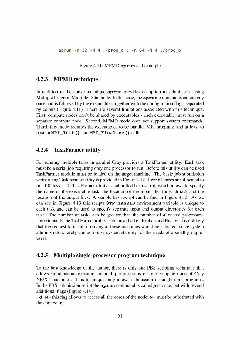
Figure 4.11: MPMD aprun call example

4.2.3 MPMD technique

In addition to the above technique aprun provides an option to submit jobs usingMultiple Program Multiple Data mode. In this case, the aprun command is called onlyonce and is followed by the executables together with the configuration flags, separatedby colons (Figure 4.11). There are several limitations associated with this technique.First, compute nodes can’t be shared by executables - each executable must run on aseparate compute node. Second, MPMD mode does not support system commands.Third, this mode requires the executables to be parallel MPI programs and at least topost an MPI_Init() and MPI_Finalize() calls.

4.2.4 TaskFarmer utility

For running multiple tasks in parallel Cray provides a TaskFarmer utility. Each taskmust be a serial job requiring only one processor to run. Before this utility can be usedTaskFarmer module must be loaded on the target machine. The basic job submissionscript using TaskFarmer utility is provided in Figure 4.12. Here 64 cores are allocated torun 100 tasks. To TaskFarmer utility is submitted bash script, which allows to specifythe name of the executable task, the location of the input files for each task and thelocation of the output files. A sample bash script can be find in Figure 4.13. As wecan see in Figure 4.13 this scripts $TF_TASKID environment variable is unique toeach task and can be used to specify separate input and output directories for eachtask. The number of tasks can be greater than the number of allocated processors.Unfortunately the TaskFarmer utility is not installed on Kraken and Hector. It is unlikelythat the request to install it on any of these machines would be satisfied, since systemadministrators rarely comporomise system stability for the needs of a small group ofusers.

4.2.5 Multiple single-processor program technique

To the best knowledge of the author, there is only one PBS scripting technique thatallows simultaneous execution of multiple programs on one compute node of CrayXE/XT machines. This technique only allows submission of single core programs.In the PBS submission script the aprun command is called just once, but with severaladditional flags (Figure 4.14):-d N - this flag allows to access all the cores of the node; N - must be substituted withthe core count

51

Figure 4.12: PBS script using TaskFarmer utility

Figure 4.13: my_task.sh example bash script for TaskFarmer utility

52

Figure 4.14: PBS example script for running multiple single-processor jobs

-cc none - this enables each program to run on a separate core-a xt - enables aprun to run script instead of a programIn addition to that, aprun command must be followed by the -n 1 flag, ensuring thateach program would run on a single core. Script that is submitted instead of executableis a simple shell script (Figure 4.15), in which required number of single-core programsis specified. It is important to note that it is possible to specify any number of executa-bles that would not exceed total core count of a given node. This technique was provento work on both Hector and Kraken using conventional PBS scripts.It is possible to use this technique with BigJob, with minor changes to the source code,which take into account additional aprun flags. In order to use this technique, after in-stalling modified version of BigJob, users only have to write a simple shell script whererequired number of single-core executables is specified.

53

Figure 4.15: Example shell script for running multiple single-processor jobs

54

Chapter 5

Conclusions

5.1 NAMD ASyncRE module

This MSc dissertation involved implementation of the NAMD based module for ASyn-cRE Python package. Implemented NAMD module supports Temperature Exchangeand Umbrella Sampling RE schemes. Current implementation of RE-US scheme sup-ports only one dimensional simulations. In order to support multi-dimensional RE-USschemes only minor code alternations would be required since current one-dimensionalimplementation is based on core NAMD configuration file which is used for both schemes.NAMD implementation of RE-US scheme demonstrated performance comparable withASyncRE Amber module. At the same time NAMD implementations of both REschemes were significantly slower than conventional NAMD. Despite this fact for suf-ficiently complex systems requiring significant amount of computational power, ASyn-cRE NAMD module potentially can be competitive with conventional NAMD simula-tions. Even if differentce in average simulation speeds still would be significant, dueto better sampling of the asynchronous RE model, ASyncRE module would require toperform fewer time-steps to arrive to solution.

5.2 BigJob on Cray machines

During this dissertation project, was made an attempt to develop a solution that wouldovercome limitation imposed by aprun on Cray machines, which only allows to launchone executable per node at any given time. A number of possible solutions were ex-amined, including parallelization of BigJob with mpi4py. The only working solutionidentified was multiple single-processor program scripting technique. This solution wasproven to work using conventional PBS scripts on both Hector and Kraken. In additionto that this solution was implemented in BigJob. Due to time limitations it was notpossible to fully test this implementation. Unfortunately, even if implementation of this

55

technique would be fully functional, it would not be possible to use it for RE simualtionswith ASyncRE due to specifics of this package.

5.3 Future work

5.3.1 NAMD ASyncRE module

A very important improvement that would greatly complement developed NAMD mod-ule for ASyncRE package is a dedicated input/output (i/o) module. In current imple-mentation of NAMD module, much of the complexity is handled by NAMD tcl scripts.As the result, input scripts are relatively complex and cumbersome for inexperienceduser to understand. All required data is extracted from NAMD during the simulationand exchange decisions are made by manipulating this data. Arguably a better approachwould be to develop a dedicated i/o module, which would allow to perform Python func-tion calls in order to extract needed simulation data. For temperature-exchange schemethis may not be of a great importance, since all required data values can be easily redi-rected to .history file, but for RE Umbrella Sampling and other more complicatedschemes i/o module would provide a convenient way to extract required data after thesimulation has finished.Another important improvement would be enabling functionality to specify the requiredsimulation length (number of time-steps) for all replicas. Currently NAMD module suf-fers from overheads associated with specifying cycle length as a wall clock time.

5.3.2 Gromacs ASyncRE module

As described above another candidate application for writing an ASyncRE extensionmodule was Gromacs. Implementing a Gromacs ASyncRE module would be a use-ful exercise for several reasons. First, it would allow to compare the learning curvesfor NAMD and Gromacs, since author of this paper didn’t had any experience withany of those programs. Next, it would allow to compare amount of effort required todecompose existing simulation setup and to write the ASyncRE module itself. Evenfor existing Impact and Amber modules the amount of coding effort spent for writing amodule for a single schema is vastly different, with Amber requiring several times moredeveloper effort than Impact. Of course the choice of schema has some efects on therequired coding effort, but even comparing the number of lines of code required, thiseffect is negligible. Another advantage of implementing a Gromacs ASyncRE moduleis possibility to identify some flaws in existing core module or some incorrect assump-tions in how extension modules can be implemented.

56

Appendix A

Stuff which is too detailed

A.0.3 BigJob example script (Kraken)

from p i l o t i m p o r t P i l o t C o m p u t e S e r v i c e , ComputeDataServ ice , S t a t ei m p o r t os , t ime , s y s

NUMBER_JOBS = 4COORDINATION_URL = " r e d i s : / / k raken−g s i 3 : 6 3 7 9 "

p i l o t _ c o m p u t e _ s e r v i c e = P i l o t C o m p u t e S e r v i c e (COORDINATION_URL)

p i l o t _ c o m p u t e _ d e s c r i p t i o n ={" s e r v i c e _ u r l " : " pbs : / / l o c a l h o s t " ," n u m b e r _ o f _ p r o c e s s e s " : 24 ," queue " : " s m a l l " ," a l l o c a t i o n " : "TG−MCB090174 " ," p r o c e s s e s _ p e r _ n o d e " : 2 ," w o r k i n g _ d i r e c t o r y " : " / l u s t r e / s c r a t c h / a n t o n t r e / b j / a g e n t " ," w a l l t i m e " : 1 0

}

p i l o t j o b = \p i l o t _ c o m p u t e _ s e r v i c e . c r e a t e _ p i l o t ( p i l o t _ c o m p u t e _ d e s c r i p t i o n = \p i l o t _ c o m p u t e _ d e s c r i p t i o n )

c o m p u t e _ d a t a _ s e r v i c e = ComputeDa taServ ice ( )c o m p u t e _ d a t a _ s e r v i c e . a d d _ p i l o t _ c o m p u t e _ s e r v i c e ( p i l o t _ c o m p u t e _ s e r v i c e )

57

# s t a r t work u n i tc o m p u t e _ u n i t _ d e s c r i p t i o n = {

" e x e c u t a b l e " : " / l u s t r e / s c r a t c h / a n t o n t r e / b j / example−mpi " ," a rgumen t s " : [ " " ] ," n u m b e r _ o f _ p r o c e s s e s " : 1 ," o u t p u t " : " s t d o u t . t x t " ," e r r o r " : " s t d e r r . t x t " ,

}

f o r i i n r a n g e (NUMBER_JOBS ) :c o m p u t e _ u n i t = \c o m p u t e _ d a t a _ s e r v i c e . s u b m i t _ c o m p u t e _ u n i t ( c o m p u t e _ u n i t _ d e s c r i p t i o n )

c o m p u t e _ d a t a _ s e r v i c e . w a i t ( )

c o m p u t e _ d a t a _ s e r v i c e . c a n c e l ( )

A.0.4 NAMD RE with Temperature Exchange example script- replica.namd

r e p l i c a B a r r i e r

s e t n r [ numRepl icas ]i f { $ n u m _ r e p l i c a s != $nr } {

e r r o r " r e s t a r t w i th wrong number o f r e p l i c a s "}s e t r [ myRepl ica ]s e t r e p l i c a _ i d $ r

i f { [ i n f o e x i s t s r e s t a r t _ r o o t ] } { # r e s t a r ts e t r e s t a r t _ r o o t [ f o r m a t $ r e s t a r t _ r o o t $ r e p l i c a _ i d ]s o u r c e $ r e s t a r t _ r o o t . $ r e p l i c a _ i d . t c l

} e l s e {s e t i _ j o b 0s e t i _ r u n 0s e t i _ s t e p 0i f { [ i n f o e x i s t s f i r s t _ t i m e s t e p ] } {

s e t i _ s t e p $ f i r s t _ t i m e s t e p}

s e t r e p l i c a ( i n d e x ) $ rs e t r e p l i c a ( l o c . a ) $ rs e t r e p l i c a ( i n d e x . a ) $ rs e t r e p l i c a ( l o c . b ) $ r

58

s e t r e p l i c a ( i n d e x . b ) $ rs e t r e p l i c a ( e x c h a n g e s _ a t t e m p t e d ) 0s e t r e p l i c a ( e x c h a n g e s _ a c c e p t e d ) 0

i f { $ r % 2 == 0 && $r +1 < $nr } {s e t r e p l i c a ( l o c . a ) [ exp r $ r +1]s e t r e p l i c a ( i n d e x . a ) [ exp r $ r +1]

}i f { $ r % 2 == 1 && $r > 0 } {

s e t r e p l i c a ( l o c . a ) [ exp r $r−1]s e t r e p l i c a ( i n d e x . a ) [ exp r $r−1]

}

i f { $ r % 2 == 1 && $r +1 < $nr } {s e t r e p l i c a ( l o c . b ) [ exp r $ r +1]s e t r e p l i c a ( i n d e x . b ) [ exp r $ r +1]

}i f { $ r % 2 == 0 && $r > 0 } {

s e t r e p l i c a ( l o c . b ) [ exp r $r−1]s e t r e p l i c a ( i n d e x . b ) [ exp r $r−1]

}

}

s e t j o b _ o u t p u t _ r o o t " $ o u t p u t _ r o o t . j o b $ i _ j o b "f i r s t t i m e s t e p $ i _ s t e p

p roc r e p l i c a _ t e m p { i } {g l o b a l n u m _ r e p l i c a s min_temp max_tempr e t u r n [ f o r m a t "%.2 f " [ exp r ( $min_temp ∗ \

exp ( l o g ( 1 . 0 ∗ $max_temp / $min_temp )∗ \( 1 . 0 ∗ $ i / ( $ n u m _ r e p l i c a s −1)) ) ) ] ]

}

s e t r e p l i c a ( t e m p e r a t u r e ) [ r e p l i c a _ t e m p $ r e p l i c a ( i n d e x ) ]s e t r e p l i c a ( t e m p e r a t u r e . a ) [ r e p l i c a _ t e m p $ r e p l i c a ( i n d e x . a ) ]s e t r e p l i c a ( t e m p e r a t u r e . b ) [ r e p l i c a _ t e m p $ r e p l i c a ( i n d e x . b ) ]

p roc s a v e _ c a l l b a c k { l a b e l s v a l u e s } {g l o b a l s a v e d _ l a b e l s s a v e d _ v a l u e ss e t s a v e d _ l a b e l s $ l a b e l ss e t s a v e d _ v a l u e s $ v a l u e s

}c a l l b a c k s a v e _ c a l l b a c k

59

p roc s a v e _ a r r a y {} {g l o b a l s a v e d _ l a b e l s s a v e d _ v a l u e s s a v e d _ a r r a yf o r e a c h l a b e l $ s a v e d _ l a b e l s v a l u e $ s a v e d _ v a l u e s {

s e t s a v e d _ a r r a y ( $ l a b e l ) $ v a l u e}

}

s e t NEWTEMP $ r e p l i c a ( t e m p e r a t u r e )s eed [ exp r i n t (0∗ s r a n d ( i n t (100000∗ r and ( ) ) + \100∗ $ r e p l i c a _ i d ) + 100000∗ r and ( ) ) ]

langevinTemp $NEWTEMPoutpu tname [ f o r m a t $ j o b _ o u t p u t _ r o o t . $ r e p l i c a _ i d $ r e p l i c a _ i d ]

i f { $ i _ r u n } { # r e s t a r tb i n c o o r d i n a t e s $ r e s t a r t _ r o o t . $ r e p l i c a _ i d . coo rb i n v e l o c i t i e s $ r e s t a r t _ r o o t . $ r e p l i c a _ i d . v e lex t endedSys t em $ r e s t a r t _ r o o t . $ r e p l i c a _ i d . xsc

} e l s e {t e m p e r a t u r e $NEWTEMP

}

o u t p u t E n e r g i e s [ exp r $ s t e p s _ p e r _ r u n / 10]dcdFreq [ exp r $ s t e p s _ p e r _ r u n ∗ $ r u n s _ p e r _ f r a m e ]

s o u r c e $ n a m d _ c o n f i g _ f i l e

s e t h i s t o r y _ f i l e [ open [ f o r m a t \" $ j o b _ o u t p u t _ r o o t . $ r e p l i c a _ i d . h i s t o r y " $ r e p l i c a _ i d ] "w" ]

f c o n f i g u r e $ h i s t o r y _ f i l e −b u f f e r i n g l i n e

w h i l e { $ i _ r u n < $num_runs } {

run $ s t e p s _ p e r _ r u ns a v e _ a r r a yi n c r i _ s t e p $ s t e p s _ p e r _ r u ns e t TEMP $ s a v e d _ a r r a y (TEMP)s e t POTENTIAL [ exp r $ s a v e d _ a r r a y (TOTAL) − $ s a v e d _ a r r a y ( KINETIC ) ]p u t s $ h i s t o r y _ f i l e " $ i _ s t e p $ r e p l i c a ( i n d e x ) \

$NEWTEMP $TEMP $POTENTIAL"

i f { $ i _ r u n % 2 == 0 } {s e t swap a ; s e t o t h e r b

60

} e l s e {s e t swap b ; s e t o t h e r a

}

s e t doswap 0i f { $ r e p l i c a ( i n d e x ) < $ r e p l i c a ( i n d e x . $swap ) } {

s e t temp $ r e p l i c a ( t e m p e r a t u r e )s e t temp2 $ r e p l i c a ( t e m p e r a t u r e . $swap )s e t BOLTZMAN 0.001987191s e t d b e t a [ exp r ( ( 1 . 0 / $temp ) − ( 1 . 0 / $temp2 ) ) / $BOLTZMAN]s e t p o t $POTENTIALs e t po t2 [ r e p l i c a R e c v $ r e p l i c a ( l o c . $swap ) ]s e t d e l t a [ exp r $ d b e t a ∗ ( $po t2 − $po t ) ]s e t doswap [ exp r $ d e l t a < 0 . | | exp (−1. ∗ $ d e l t a ) > rand ( ) ]r e p l i c a S e n d $doswap $ r e p l i c a ( l o c . $swap )i f { $doswap } {

s e t r i d $ r e p l i c a ( i n d e x )s e t r i d 2 $ r e p l i c a ( i n d e x . $swap )p u t s s t d e r r "EXCHANGE_ACCEPT $ r i d ( $temp ) \

$ r i d 2 ( $temp2 ) RUN $ i _ r u n "i n c r r e p l i c a ( e x c h a n g e s _ a c c e p t e d )

}i n c r r e p l i c a ( e x c h a n g e s _ a t t e m p t e d )

}i f { $ r e p l i c a ( i n d e x ) > $ r e p l i c a ( i n d e x . $swap ) } {

r e p l i c a S e n d $POTENTIAL $ r e p l i c a ( l o c . $swap )s e t doswap [ r e p l i c a R e c v $ r e p l i c a ( l o c . $swap ) ]

}

s e t newloc $ ri f { $doswap } {

s e t newloc $ r e p l i c a ( l o c . $swap )s e t r e p l i c a ( l o c . $swap ) $ r

}s e t r e p l i c a ( l o c . $ o t h e r ) [ r e p l i c a S e n d r e c v \

$newloc $ r e p l i c a ( l o c . $ o t h e r ) $ r e p l i c a ( l o c . $ o t h e r ) ]s e t o l d i d x $ r e p l i c a ( i n d e x )i f { $doswap } {

s e t OLDTEMP $ r e p l i c a ( t e m p e r a t u r e )a r r a y s e t r e p l i c a [ r e p l i c a S e n d r e c v [ a r r a y g e t r e p l i c a ] \

$newloc $newloc ]s e t NEWTEMP $ r e p l i c a ( t e m p e r a t u r e )r e s c a l e v e l s [ exp r s q r t ( 1 . 0 ∗$NEWTEMP/$OLDTEMP ) ]langevinTemp $NEWTEMP

61

}

# p u t s s t d e r r " i t e r a t i o n $ i _ r u n r e p l i c a \$ r e p l i c a ( i n d e x ) now on rank $r "

# r e p l i c a B a r r i e r

i n c r i _ r u n

i f { $ i _ r u n % ( $ r u n s _ p e r _ f r a m e ∗ $ f r a m e s _ p e r _ r e s t a r t ) == 0 | |$ i _ r u n == $num_runs } { # r e s t a r t

s e t r e s t a r t _ r o o t " $ j o b _ o u t p u t _ r o o t . r e s t a r t $ i _ r u n "o u t p u t [ f o r m a t $ r e s t a r t _ r o o t . $ r e p l i c a _ i d $ r e p l i c a _ i d ]s e t r f i l e [ open [ f o r m a t " $ r e s t a r t _ r o o t . $ r e p l i c a _ i d . t c l " \

$ r e p l i c a _ i d ] "w" ]p u t s $ r f i l e [ l i s t a r r a y s e t r e p l i c a [ a r r a y g e t r e p l i c a ] ]c l o s e $ r f i l er e p l i c a B a r r i e ri f { $ r e p l i c a _ i d == 0 } {

s e t r f i l e [ open [ f o r m a t " $ r e s t a r t _ r o o t . t c l " " " ] "w" ]p u t s $ r f i l e [ l i s t s e t i _ j o b [ exp r $ i _ j o b + 1 ] ]p u t s $ r f i l e [ l i s t s e t i _ r u n $ i _ r u n ]p u t s $ r f i l e [ l i s t s e t i _ s t e p $ i _ s t e p ]p u t s $ r f i l e [ l i s t s e t r e s t a r t _ r o o t $ r e s t a r t _ r o o t ]c l o s e $ r f i l ei f [ i n f o e x i s t s o l d _ r e s t a r t _ r o o t ] {

s e t o l d r o o t [ f o r m a t $ o l d _ r e s t a r t _ r o o t " " ]f i l e d e l e t e $ o l d r o o t . t c l

}}r e p l i c a B a r r i e ri f [ i n f o e x i s t s o l d _ r e s t a r t _ r o o t ] {

s e t o l d r o o t [ f o r m a t $ o l d _ r e s t a r t _ r o o t $ r e p l i c a _ i d ]f i l e d e l e t e $ o l d r o o t . $ r e p l i c a _ i d . t c lf i l e d e l e t e $ o l d r o o t . $ r e p l i c a _ i d . coo rf i l e d e l e t e $ o l d r o o t . $ r e p l i c a _ i d . v e lf i l e d e l e t e $ o l d r o o t . $ r e p l i c a _ i d . xsc

}s e t o l d _ r e s t a r t _ r o o t $ r e s t a r t _ r o o t

}}

s e t a t t e m p t s $ r e p l i c a ( e x c h a n g e s _ a t t e m p t e d )i f $ a t t e m p t s {

s e t i $ r e p l i c a ( i n d e x )

62

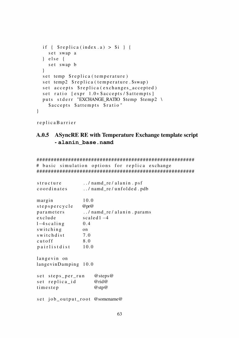
i f { $ r e p l i c a ( i n d e x . a ) > $ i } {s e t swap a

} e l s e {s e t swap b

}s e t temp $ r e p l i c a ( t e m p e r a t u r e )s e t temp2 $ r e p l i c a ( t e m p e r a t u r e . $swap )s e t a c c e p t s $ r e p l i c a ( e x c h a n g e s _ a c c e p t e d )s e t r a t i o [ exp r 1 . 0∗ $ a c c e p t s / $ a t t e m p t s ]p u t s s t d e r r "EXCHANGE_RATIO $temp $temp2 \

$ a c c e p t s $ a t t e m p t s $ r a t i o "}

r e p l i c a B a r r i e r

A.0.5 ASyncRE RE with Temperature Exchange template script- alanin_base.namd

######################################################## b a s i c s i m u l a t i o n o p t i o n s f o r r e p l i c a exchange#######################################################

s t r u c t u r e . . / namd_re / a l a n i n . p s fc o o r d i n a t e s . . / namd_re / u n f o l d e d . pdb

margin 1 0 . 0s t e p s p e r c y c l e @pr@p a r a m e t e r s . . / namd_re / a l a n i n . paramse x c l u d e s c a l e d 1 −41−4 s c a l i n g 0 . 4s w i t c h i n g ons w i t c h d i s t 7 . 0c u t o f f 8 . 0p a i r l i s t d i s t 1 0 . 0

l a n g e v i n onlangev inDamping 1 0 . 0

s e t s t e p s _ p e r _ r u n @steps@s e t r e p l i c a _ i d @rid@t i m e s t e p @stp@

s e t j o b _ o u t p u t _ r o o t @somename@

63

s e t o l d _ o u t p u t _ r o o t @oldname@

s e t i _ r u n @cycle@f i r s t t i m e s t e p @ f i r s t s t e p @

s e t c y c l e [ exp r $ i _ r u n +1]s e t doswap @swap@

s e t ou tpu tname $ j o b _ o u t p u t _ r o o t $ c y c l eoutputName $outpu tname

s e t OLDTEMP @ot@s e t NEWTEMP @nt@

i f { $ i _ r u n } { # r e s t a r ts e t o l d r u n [ exp r ( $cyc l e −1)]s e t o l d o u t p u t $ o l d _ o u t p u t _ r o o t $ o l d r u nb i n c o o r d i n a t e s $ o l d o u t p u t . coo rb i n v e l o c i t i e s $ o l d o u t p u t . v e lex t endedSys t em $ o l d o u t p u t . xsc

} e l s e {t e m p e r a t u r e $NEWTEMP

}

o u t p u t E n e r g i e s [ exp r ( $ s t e p s _ p e r _ r u n / 1 0 ) ]dcdFreq [ exp r ( $ s t e p s _ p e r _ r u n ∗ 1 0 ) ]

i f { $doswap } {r e s c a l e v e l s [ exp r s q r t ( 1 . 0 ∗$NEWTEMP/$OLDTEMP ) ]

}langevinTemp $NEWTEMP

######################################################## t h i s b l o c k i s f o r p u t t i n g o u t p u t i n t o h i s t o r y f i l e#######################################################

p roc s a v e _ c a l l b a c k { l a b e l s v a l u e s } {g l o b a l s a v e d _ l a b e l s s a v e d _ v a l u e ss e t s a v e d _ l a b e l s $ l a b e l ss e t s a v e d _ v a l u e s $ v a l u e s

}c a l l b a c k s a v e _ c a l l b a c k

p roc s a v e _ a r r a y {} {

64

g l o b a l s a v e d _ l a b e l s s a v e d _ v a l u e s s a v e d _ a r r a yf o r e a c h l a b e l $ s a v e d _ l a b e l s v a l u e $ s a v e d _ v a l u e s {

s e t s a v e d _ a r r a y ( $ l a b e l ) $ v a l u e}

}

s e t h i s t o r y _ f i l e [ open [ f o r m a t " @history@ " ] "w" ]f c o n f i g u r e $ h i s t o r y _ f i l e −b u f f e r i n g l i n e

#######################################################

run $ s t e p s _ p e r _ r u ns a v e _ a r r a y

s e t TEMP $ s a v e d _ a r r a y (TEMP)s e t POTENTIAL [ exp r $ s a v e d _ a r r a y (TOTAL) − $ s a v e d _ a r r a y ( KINETIC ) ]

p u t s $ h i s t o r y _ f i l e "$NEWTEMP $POTENTIAL"

A.0.6 NAMD RE with Umbrella Sampling example script- umbrella.namd

# v a l i d a t e r e p l i c a _ n e i g h b o r s p roc − works i n t c l s hf o r { s e t i 0 } { $ i < $ n u m _ r e p l i c a s } { i n c r i } {

s e t j 0f o r e a c h nbr [ r e p l i c a _ n e i g h b o r s $ i ] {

i f { $nbr < 0 } {e r r o r " r e p l i c a _ n e i g h b o r s i n c o n s i s t e n c y d e t e c t e d : \n e i g h b o r $ j o f r e p l i c a $ i i s $nbr b u t s h o u l d n o t \be n e g a t i v e "

}i f { $nbr >= $ n u m _ r e p l i c a s } {

e r r o r " r e p l i c a _ n e i g h b o r s i n c o n s i s t e n c y d e t e c t e d : \n e i g h b o r $ j o f r e p l i c a $ i i s $nbr b u t t h e r e a r e \on ly $ n u m _ r e p l i c a s r e p l i c a s "

}s e t r n b r l [ r e p l i c a _ n e i g h b o r s $nbr ]s e t r n b r c [ l l e n g t h $ r n b r l ]i f { $ j >= $ r n b r c } {

e r r o r " r e p l i c a _ n e i g h b o r s i n c o n s i s t e n c y d e t e c t e d : \n e i g h b o r $ j o f r e p l i c a $ i i s $nbr b u t r e p l i c a \$nbr has on ly $ r n b r c n e i g h b o r s "

}

65

s e t r n b r [ l i n d e x $ r n b r l $ j ]i f { $ r n b r != $ i } {

e r r o r " r e p l i c a _ n e i g h b o r s i n c o n s i s t e n c y d e t e c t e d : \n e i g h b o r $ j o f r e p l i c a $ i i s $nbr b u t n e i g h b o r $ j \o f r e p l i c a $nbr i s $ r n b r "

}i n c r j

}}p u t s " r e p l i c a _ n e i g h b o r s p roc p a s s e s i n t e r n a l c o n s i s t check "

# b a i l i f t h i s i s n o t NAMDi f { [ c a t c h numPes ] } {

p u t s " Tc l i n t e r p r e t e r does n o t a p p e a r t o be NAMD \− s c r i p t e x i t i n g "r e t u r n

}

r e p l i c a B a r r i e r

s e t n r [ numRepl icas ]i f { $ n u m _ r e p l i c a s != $nr } {

e r r o r " r e s t a r t w i th wrong number o f r e p l i c a s "}s e t r [ myRepl ica ]s e t r e p l i c a _ i d $ r

i f { [ i n f o e x i s t s r e s t a r t _ r o o t ] } { # r e s t a r ts e t r e s t a r t _ r o o t [ f o r m a t $ r e s t a r t _ r o o t $ r e p l i c a _ i d ]s o u r c e $ r e s t a r t _ r o o t . $ r e p l i c a _ i d . t c l

} e l s e {s e t i _ j o b 0s e t i _ r u n 0s e t i _ s t e p 0i f { [ i n f o e x i s t s f i r s t _ t i m e s t e p ] } {

s e t i _ s t e p $ f i r s t _ t i m e s t e p}

s e t r e p l i c a ( i n d e x ) $ rs e t nnbr 0f o r e a c h nbr [ r e p l i c a _ n e i g h b o r s $ r ] {

s e t r e p l i c a ( l o c . $nnbr ) $nbrs e t r e p l i c a ( i n d e x . $nnbr ) $nbrs e t r e p l i c a ( e x c h a n g e s _ a t t e m p t e d . $nnbr ) 0

66

s e t r e p l i c a ( e x c h a n g e s _ a c c e p t e d . $nnbr ) 0i n c r nnbr

}s e t r e p l i c a ( num_neighbors ) $nnbr

}

s e t j o b _ o u t p u t _ r o o t " $ o u t p u t _ r o o t . j o b $ i _ j o b "f i r s t t i m e s t e p $ i _ s t e p

s e t r e p l i c a ( c o l v a r b i a s ) [ r e p l i c a _ b i a s $ r e p l i c a ( i n d e x ) ]f o r { s e t i 0 } { $ i < $ r e p l i c a ( num_neighbors ) } { i n c r i } {

s e t r e p l i c a ( c o l v a r b i a s . $ i ) [ r e p l i c a _ b i a s $ r e p l i c a ( i n d e x . $ i ) ]s e t r e p l i c a ( c o l v a r b i a s . $ i ) [ r e p l i c a _ b i a s $ r e p l i c a ( i n d e x . $ i ) ]

}

p roc s a v e _ c a l l b a c k { l a b e l s v a l u e s } {g l o b a l s a v e d _ l a b e l s s a v e d _ v a l u e ss e t s a v e d _ l a b e l s $ l a b e l ss e t s a v e d _ v a l u e s $ v a l u e s

}c a l l b a c k s a v e _ c a l l b a c k

p roc s a v e _ a r r a y {} {g l o b a l s a v e d _ l a b e l s s a v e d _ v a l u e s s a v e d _ a r r a yf o r e a c h l a b e l $ s a v e d _ l a b e l s v a l u e $ s a v e d _ v a l u e s {

s e t s a v e d _ a r r a y ( $ l a b e l ) $ v a l u e}

}

seed [ exp r i n t (0∗ s r a n d ( i n t (100000∗ r and ( ) ) + \100∗ $ r e p l i c a _ i d ) + 100000∗ r and ( ) ) ]ou tpu tname [ f o r m a t $ j o b _ o u t p u t _ r o o t . $ r e p l i c a _ i d $ r e p l i c a _ i d ]

i f { $ i _ r u n } { # r e s t a r tb i n c o o r d i n a t e s $ r e s t a r t _ r o o t . $ r e p l i c a _ i d . coo rb i n v e l o c i t i e s $ r e s t a r t _ r o o t . $ r e p l i c a _ i d . v e lex t endedSys t em $ r e s t a r t _ r o o t . $ r e p l i c a _ i d . xscc o l v a r s I n p u t $ r e s t a r t _ r o o t . $ r e p l i c a _ i d . c o l v a r s . s t a t e

} e l s e i f { [ i n f o e x i s t s i n p u t _ r o o t ] } {s e t i r [ f o r m a t $ i n p u t _ r o o t $ r e p l i c a _ i d $ r e p l i c a _ i d ]b i n c o o r d i n a t e s $ i r . coo rb i n v e l o c i t i e s $ i r . v e lex t endedSys t em $ i r . xsc

} e l s e {

67

t e m p e r a t u r e $ t e m p e r a t u r e}

o u t p u t E n e r g i e s [ exp r $ s t e p s _ p e r _ r u n / 10]dcdFreq [ exp r $ s t e p s _ p e r _ r u n ∗ $ r u n s _ p e r _ f r a m e ]

s o u r c e $ n a m d _ c o n f i g _ f i l e

e v a l c o l v a r b i a s [ c o n c a t c h a n g e c o n f i g $ r e p l i c a ( c o l v a r b i a s ) ]

s e t h i s t o r y _ f i l e [ open [ f o r m a t \" $ j o b _ o u t p u t _ r o o t . $ r e p l i c a _ i d . h i s t o r y " $ r e p l i c a _ i d ] "w" ]f c o n f i g u r e $ h i s t o r y _ f i l e −b u f f e r i n g l i n e

w h i l e { $ i _ r u n < $num_runs } {

run $ s t e p s _ p e r _ r u ns a v e _ a r r a yi n c r i _ s t e p $ s t e p s _ p e r _ r u ns e t TEMP $ s a v e d _ a r r a y (TEMP)s e t POTENTIAL [ exp r $ s a v e d _ a r r a y (TOTAL) − $ s a v e d _ a r r a y ( KINETIC ) ]p u t s $ h i s t o r y _ f i l e " $ i _ s t e p $ r e p l i c a ( i n d e x ) $TEMP $POTENTIAL"

s e t swap [ exp r $ i _ r u n % $ r e p l i c a ( num_neighbors ) ]

s e t doswap 0i f { $ r e p l i c a ( i n d e x ) < $ r e p l i c a ( i n d e x . $swap ) } {

s e t BOLTZMAN 0.001987191s e t e d i f f [ e v a l c o l v a r b i a s [ c o n c a t e n e r g y d i f f \$ r e p l i c a ( c o l v a r b i a s . $swap ) ] ]s e t e d i f f 2 [ r e p l i c a R e c v $ r e p l i c a ( l o c . $swap ) ]s e t d e l t a [ exp r ( $ e d i f f + $ e d i f f 2 ) / ( $BOLTZMAN ∗ $ t e m p e r a t u r e ) ]s e t doswap [ exp r $ d e l t a < 0 . | | exp (−1. ∗ $ d e l t a ) > rand ( ) ]r e p l i c a S e n d $doswap $ r e p l i c a ( l o c . $swap )i f { $doswap } {

s e t r i d $ r e p l i c a ( i n d e x )s e t r i d 2 $ r e p l i c a ( i n d e x . $swap )p u t s s t d e r r "EXCHANGE_ACCEPT $ r i d $ r i d 2 RUN $ i _ r u n "i n c r r e p l i c a ( e x c h a n g e s _ a c c e p t e d . $swap )

}i n c r r e p l i c a ( e x c h a n g e s _ a t t e m p t e d . $swap )

}i f { $ r e p l i c a ( i n d e x ) > $ r e p l i c a ( i n d e x . $swap ) } {

s e t e d i f f [ e v a l c o l v a r b i a s [ c o n c a t e n e r g y d i f f \

68

$ r e p l i c a ( c o l v a r b i a s . $swap ) ] ]r e p l i c a S e n d $ e d i f f $ r e p l i c a ( l o c . $swap )s e t doswap [ r e p l i c a R e c v $ r e p l i c a ( l o c . $swap ) ]

}

s e t newloc $ ri f { $doswap } {

s e t newloc $ r e p l i c a ( l o c . $swap )s e t r e p l i c a ( l o c . $swap ) $ r

}f o r { s e t i 0} { $ i < $ r e p l i c a ( num_neighbors ) } { i n c r i } {

i f { $ i != $swap } {s e t r e p l i c a ( l o c . $ i ) [ r e p l i c a S e n d r e c v $newloc \$ r e p l i c a ( l o c . $ i ) $ r e p l i c a ( l o c . $ i ) ]

}}s e t o l d i d x $ r e p l i c a ( i n d e x )i f { $doswap } {

a r r a y s e t r e p l i c a [ r e p l i c a S e n d r e c v \[ a r r a y g e t r e p l i c a ] $newloc $newloc ]e v a l c o l v a r b i a s [ c o n c a t c h a n g e c o n f i g $ r e p l i c a ( c o l v a r b i a s ) ]

}

i n c r i _ r u n

i f { $ i _ r u n % ( $ r u n s _ p e r _ f r a m e ∗ $ f r a m e s _ p e r _ r e s t a r t ) == 0 | |$ i _ r u n == $num_runs } { # r e s t a r t

s e t r e s t a r t _ r o o t " $ j o b _ o u t p u t _ r o o t . r e s t a r t $ i _ r u n "s e t r r o o t [ f o r m a t $ r e s t a r t _ r o o t . $ r e p l i c a _ i d $ r e p l i c a _ i d ]o u t p u t $ r r o o ts e t o r o o t [ f o r m a t $ j o b _ o u t p u t _ r o o t . $ r e p l i c a _ i d $ r e p l i c a _ i d ]f i l e rename −f o r c e $ o r o o t . c o l v a r s . s t a t e $ r r o o t . c o l v a r s . s t a t es e t r f i l e [ open [ f o r m a t " $ r e s t a r t _ r o o t . $ r e p l i c a _ i d . t c l " \$ r e p l i c a _ i d ] "w" ]p u t s $ r f i l e [ l i s t a r r a y s e t r e p l i c a [ a r r a y g e t r e p l i c a ] ]c l o s e $ r f i l er e p l i c a B a r r i e ri f { $ r e p l i c a _ i d == 0 } {

s e t r f i l e [ open [ f o r m a t " $ r e s t a r t _ r o o t . t c l " " " ] "w" ]p u t s $ r f i l e [ l i s t s e t i _ j o b [ exp r $ i _ j o b + 1 ] ]p u t s $ r f i l e [ l i s t s e t i _ r u n $ i _ r u n ]p u t s $ r f i l e [ l i s t s e t i _ s t e p $ i _ s t e p ]p u t s $ r f i l e [ l i s t s e t r e s t a r t _ r o o t $ r e s t a r t _ r o o t ]c l o s e $ r f i l e

69

i f [ i n f o e x i s t s o l d _ r e s t a r t _ r o o t ] {s e t o l d r o o t [ f o r m a t $ o l d _ r e s t a r t _ r o o t " " ]f i l e d e l e t e $ o l d r o o t . t c l

}}r e p l i c a B a r r i e ri f [ i n f o e x i s t s o l d _ r e s t a r t _ r o o t ] {

s e t o l d r o o t [ f o r m a t $ o l d _ r e s t a r t _ r o o t $ r e p l i c a _ i d ]f i l e d e l e t e $ o l d r o o t . $ r e p l i c a _ i d . t c lf i l e d e l e t e $ o l d r o o t . $ r e p l i c a _ i d . coo rf i l e d e l e t e $ o l d r o o t . $ r e p l i c a _ i d . v e lf i l e d e l e t e $ o l d r o o t . $ r e p l i c a _ i d . xscf i l e d e l e t e $ o l d r o o t . $ r e p l i c a _ i d . c o l v a r s . s t a t e

}s e t o l d _ r e s t a r t _ r o o t $ r e s t a r t _ r o o t

}}

f o r { s e t i 0 } { $ i < $ r e p l i c a ( num_neighbors ) } { i n c r i } {s e t a t t e m p t s $ r e p l i c a ( e x c h a n g e s _ a t t e m p t e d . $ i )i f $ a t t e m p t s {

s e t a c c e p t s $ r e p l i c a ( e x c h a n g e s _ a c c e p t e d . $ i )s e t r a t i o [ exp r 1 . 0∗ $ a c c e p t s / $ a t t e m p t s ]p u t s s t d e r r "EXCHANGE_RATIO $ r e p l i c a ( i n d e x ) \$ r e p l i c a ( i n d e x . $ i ) $ a c c e p t s $ a t t e m p t s $ r a t i o "

}}

r e p l i c a B a r r i e r

A.0.7 ASyncRE RE with Umbrella Sampling template script- alanin_base_umbrella.namd

# s i m u l a t i o n o p t i o n s f o r r e p l i c a exchange

s t r u c t u r e . . / namd_us / a l a n i n . p s fc o o r d i n a t e s . . / namd_us / a l a n i n . pdb

margin 1 0 . 0s t e p s p e r c y c l e @pr@p a r a m e t e r s . . / namd_us / a l a n i n . paramse x c l u d e s c a l e d 1 −41−4 s c a l i n g 0 . 4

70

s w i t c h i n g ons w i t c h d i s t 7 . 0c u t o f f 8 . 0p a i r l i s t d i s t 1 0 . 0

c o l v a r s onc o l v a r s C o n f i g . . / namd_us / c o l v a r s . con f

l a n g e v i n onlangev inDamping 1 0 . 0

s e t s t e p s _ p e r _ r u n @steps@s e t r e p l i c a _ i d @rid@s e t b i a s _ i d @bid@t i m e s t e p @stp@s e t n u m _ r e p l i c a s @replicas@

s e t j o b _ o u t p u t _ r o o t @somename@s e t o l d _ o u t p u t _ r o o t @oldname@

s e t i _ r u n @cycle@f i r s t t i m e s t e p @ f i r s t s t e p @s e t r _ t e m p e r a t u r e @temper@s e t c y c l e [ exp r $ i _ r u n +1]

langevinTemp $ r _ t e m p e r a t u r e

p roc r e p l i c a _ b i a s { i } {r e t u r n [ l i s t l e n p o t " c e n t e r s [ exp r 17 + $ i ] " ]

}

######################################################## t h i s b l o c k i s f o r p u t t i n g o u t o u t i n t o h i s t o r y f i l e#######################################################

p roc s a v e _ c a l l b a c k { l a b e l s v a l u e s } {g l o b a l s a v e d _ l a b e l s s a v e d _ v a l u e ss e t s a v e d _ l a b e l s $ l a b e l ss e t s a v e d _ v a l u e s $ v a l u e s

}c a l l b a c k s a v e _ c a l l b a c k

p roc s a v e _ a r r a y {} {g l o b a l s a v e d _ l a b e l s s a v e d _ v a l u e s s a v e d _ a r r a y

71

f o r e a c h l a b e l $ s a v e d _ l a b e l s v a l u e $ s a v e d _ v a l u e s {s e t s a v e d _ a r r a y ( $ l a b e l ) $ v a l u e

}}

s e t h i s t o r y _ f i l e [ open [ f o r m a t " @history@ " ] "w" ]f c o n f i g u r e $ h i s t o r y _ f i l e −b u f f e r i n g l i n e

# en e r gy o u t p u ts e t e n e r g y _ f i l e [ open [ f o r m a t "@energy@ " ] "w" ]f c o n f i g u r e $ e n e r g y _ f i l e −b u f f e r i n g l i n e

#######################################################

s e t r e p l i c a ( c o l v a r b i a s ) [ r e p l i c a _ b i a s $ b i a s _ i d ]

f o r { s e t i 0 } { $ i < $ n u m _ r e p l i c a s } { i n c r i } {s e t r e p l i c a ( c o l v a r b i a s . $ i ) [ r e p l i c a _ b i a s $ i ]# p u t s $ e n e r g y _ f i l e " $ i $ r e p l i c a ( c o l v a r b i a s . $ i ) "

}

seed [ exp r i n t (0∗ s r a n d ( i n t (100000∗ r and ( ) ) + \100∗ $ r e p l i c a _ i d ) + 100000∗ r and ( ) ) ]s e t ou tpu tname $ j o b _ o u t p u t _ r o o t $ c y c l eoutputName $outpu tname

s e t i n p u t _ r o o t " . . / namd_us / i n p u t / a l a n i n . i n i t i a l . $ r e p l i c a _ i d "

i f { $ i _ r u n } { # r e s t a r ts e t o l d r u n [ exp r ( $cyc l e −1)]s e t o l d o u t p u t $ o l d _ o u t p u t _ r o o t $ o l d r u nb i n c o o r d i n a t e s $ o l d o u t p u t . coo rb i n v e l o c i t i e s $ o l d o u t p u t . v e lex t endedSys t em $ o l d o u t p u t . xscc o l v a r s I n p u t $ o l d o u t p u t . c o l v a r s . s t a t e

} e l s e i f { [ i n f o e x i s t s i n p u t _ r o o t ] } {b i n c o o r d i n a t e s $ i n p u t _ r o o t . coo rb i n v e l o c i t i e s $ i n p u t _ r o o t . v e lex t endedSys t em $ i n p u t _ r o o t . xsc

} e l s e {t e m p e r a t u r e $ r _ t e m p e r a t u r e

}

72

o u t p u t E n e r g i e s [ exp r $ s t e p s _ p e r _ r u n / 10]dcdFreq [ exp r $ s t e p s _ p e r _ r u n ∗ 10]

e v a l c o l v a r b i a s [ c o n c a t c h a n g e c o n f i g $ r e p l i c a ( c o l v a r b i a s ) ]

run $ s t e p s _ p e r _ r u ns a v e _ a r r a y

f o r { s e t i 0 } { $ i < $ n u m _ r e p l i c a s } { i n c r i } {s e t e d i f f [ e v a l c o l v a r b i a s [ c o n c a t e n e r g y d i f f \$ r e p l i c a ( c o l v a r b i a s . $ i ) ] ]p u t s $ e n e r g y _ f i l e " $ e d i f f "

}

s e t TEMP $ s a v e d _ a r r a y (TEMP)s e t POTENTIAL [ exp r $ s a v e d _ a r r a y (TOTAL)− $ s a v e d _ a r r a y ( KINETIC ) ]p u t s $ h i s t o r y _ f i l e "$TEMP $POTENTIAL $ b i a s _ i d "

73

Bibliography

[1] Protein Data Bank. Online at: http://www.rcsb.org/pdb/home/home.do (refer-enced 26/07/2013)

[2] S. Kumar, C. Huang, G. Zheng, et. al. Scalable molecular dynamics with NAMDon the IBM Blue Gene/L system. IBM Journal of Research and Development,Volume 52, Issue 1.2, 2008

[3] Y. Sugita and Y. Okamoto, Replica-Exchange Molecular Dynamics Method forProtein Folding. Chem. Phys. Lett. 314, No. 1, 141-151 (1999)

[4] M. Sotomayor and K. Schulten, Single-Molecule Experiments In Vitro and InSilico. Science 316, No. 5828, 1144-1148 (2007)

[5] HECToR: UK National Supercomputing Service. Online at:http://www.hector.ac.uk/ (referenced 26/07/2013)

[6] The National Institute for Computational Sciences: Kraken.Online at: http://www.nics.tennessee.edu/computing-resources/kraken (refer-enced 26/07/2013)

[7] NAMD - Scalable Molecular Dynamics.Online at: http://www.ks.uiuc.edu/Research/namd/ (referenced 24/07/2013)

[8] Y. Sugita, A. Kitao, Y. Okamoto, Multidimensional replica-exchange method forfree-energy calculations J. Chem. Phys. 113, 2000

[9] R. H. Swendsen and J.-S. Wang, Replica Monte Carlo Simulation of Spin-Glasses Phys. Rev. Lett., 1986, 57, 2607

[10] Y. Sugita, Y. Okamoto Replica-exchange molecular dynamics method for proteinfolding Chemical Physics Letters 314 1999. 141âAS151

[11] D.J. Earl and M.W. Deem Parallel Tempering: Theory, Applications, and NewPerspectives Physical Chemistry Chemical Physics, 2008

[12] N. Rathore, M. Chopra, and J. J. de Pablo Optimal allocation of replicas in par-allel tempering simulations J. Chem. Phys., 2005, 122, 024111

[13] A. Kone and D. A. Kofke Selection of temperature intervals for parallel-tempering simulations J. Chem. Phys., 2005, 122, 206101

74

[14] A. Thota, A. Luckow and S. Jha. Efficient large-scale replica-exchange simula-tions on production infrastructure. Phil. Trans. R. Soc. A 28 August 2011 vol.369 no. 1949 3318-3335

[15] N. Metropolis, A. W. Rosenbluth, M. N. Rosenbluth, A. H. Teller, and E. Teller,Equation of state calculations by fast computing machines. J. Chem. Phys. 21,1087-1092. (doi:10.1063/1.1699114) 1953

[16] Z. Li, M. Parashar, Grid-based asynchronous replica exchange. In GRID ’07:Proc. of the 8th IEEE/ACM Int. Conf. on Grid Computing, Austin, TX, 19-21September 2007, pp. 201-208. Washington, DC: IEEE Computer Society.

[17] E. Gallicchio, R. M. Levy, M. Parashar, Asynchronous replica exchange formolecular simulations. J. Comp. Chem. 29, 788-794, 2008

[18] BigJob: A Pilot-based Job and Data Management System. online at:http://saga-project.github.io/BigJob/ (referenced 13/07/2013)

[19] J. Moscicki, et. al. Diane - distributed analysis environment for grid-enabledsimulation and analysis of physics data. Nuclear Science Symposium Confer-ence Record, 2003 IEEE, vol. 3, 2003, pp. 1617 - 1620

[20] J. Frey, T. Tannenbaum, M. Livny, et. al. Condor-G: A Computation ManagementAgent for Multi-Institutional Grids. Cluster Computing, vol. 5, no. 3, pp. 237-246, July 2002

[21] I. Raicu, Y. Zhao, C. Dumitrescu, I. Foster, et. al. Falkon: A Fast and Light-Weight TasK ExecutiON Framework. in SC ’07: Proceedings of the 2007ACM/IEEE conference on Supercomputing. New York, NY, USA: ACM, 2007,pp. 1-12

[22] A. Casajus, R. Graciani, S. Paterson, and A. Tsaregorodtsev Dirac pilot frame-work and the dirac workload management system. Journal of Physics: Confer-ence Series, vol. 219, no. 6, p. 062049, 2010

[23] A. Luckow, M. Santcroos, A. Merzky, et. al. P*: A Model of Pilot Abstractions.Technical Report, 2012

[24] Distributed Resource Management Application API (DRMAA) working group,Online at: http://www.drmaa.org/ (referenced 23/07/2013)

[25] SAGA-Python project Online at: http://saga-project.github.io/saga-python/ (ref-erenced 23/07/2013)

[26] A Highly Scalable Resource Manager - SLURM Online at:https://computing.llnl.gov/linux/slurm/ (referenced 23/07/2013)

[27] Redis key-value store, Online at: http://redis.io/ (referenced 23/07/2013)

[28] BigJob based Asynchronous Replica-Exchange Framework.Online at: https://github.com/saga-project/asyncre-bigjob (referenced26/07/2013)

75

[29] A. Luckow, L. Lacinski, S. Jha. SAGA BigJob: An Extensible and InteroperablePilot-Job Abstraction for Distributed Applications and Systems 10th IEEE/ACMInternational Conference on Cluster, Cloud and Grid Computing. Pp 135-144,2010

[30] Assisted Model Building with Energy Refinement. Online at: http://ambermd.org/(referenced 26/07/2013)

[31] IMPACT: Molecular Simulation Program.Online at: http://hpcp.rutgers.edu/ emilio/software.shtml#impact (referenced26/07/2013)

[32] B. K. Radak, E. Gallicchio, M. Romanus, et. al. A Framework for Flexibleand Scalable Replica-Exchange on Production Distributed CI. Technical Report.XSEDE13: Gateway to Discovery, 2013

[33] Extreme Science and Engineering Discovery Environment.Online at: https://www.xsede.org/ (referenced 26/07/2013)

[34] Gromacs - GROningen MAchine for Chemical Simulations.Online at: http://www.gromacs.org/ (referenced 26/07/2013)

[35] LAMMPS - Large-scale Atomic/Molecular Massively Parallel Simulator.Online at: http://lammps.sandia.gov/ (referenced 26/07/2013)

[36] Desmond - Molecular Dynamics software package.Online at: http://www.deshawresearch.com/resources_desmond.html (refer-enced 26/07/2013)

[37] A.F.M. Smith and G.O. Roberts, Bayesian computation via the Gibbs samplerand related Markov chain Monte Carlo methods Journal of the Royal StatisticalSociety. Series B (Methodological) Vol. 55, No. 1, 1993, pp. 3-23

[38] MPI for Python - mpi4py. Online at: http://mpi4py.scipy.org/ (referenced26/07/2013)

76