1

Big Learning with Bayesian MethodsJun Zhu, Jianfei Chen, Wenbo Hu, Bo Zhang

Abstract—The explosive growth in data volume and the availability of cheap computing resources have sparked increasinginterest in Big learning, an emerging subfield that studies scalable machine learning algorithms, systems, and applications withBig Data. Bayesian methods represent one important class of statistical methods for machine learning, with substantial recentdevelopments on adaptive, flexible and scalable Bayesian learning. This article provides a survey of the recent advances inBig learning with Bayesian methods, termed Big Bayesian Learning, including nonparametric Bayesian methods for adaptivelyinferring model complexity, regularized Bayesian inference for improving the flexibility via posterior regularization, and scalablealgorithms and systems based on stochastic subsampling and distributed computing for dealing with large-scale applications.We also provide various new perspectives on the large-scale Bayesian modeling and inference.

Index Terms—Big Bayesian Learning, Bayesian nonparametrics, Regularized Bayesian inference, Scalable algorithms

F

1 INTRODUCTION

W E live in an era of Big Data, where science, engi-neering and technology are producing massive

data streams, with petabyte and exabyte scales becom-ing increasingly common [43], [56], [151]. Besides theexplosive growth in volume, Big Data also has highvelocity, high variety, and high uncertainty. Thesecomplex data streams require ever-increasing process-ing speeds, economical storage, and timely responsefor decision making in highly uncertain environments,and have raised various challenges to conventionaldata analysis [63].

With the primary goal of building intelligent sys-tems that automatically improve from experiences,machine learning (ML) is becoming an increasinglyimportant field to tackle the big data challenges [130],with an emerging field of Big Learning, which coverstheories, algorithms and systems on addressing bigdata problems.

1.1 Big Learning ChallengesIn big data era, machine learning needs to deal withthe challenges of learning from complex situationswith large N , large P , large L, and large M , where Nis the data size, P is the feature dimension, L is thenumber of tasks, and M is the model size. Given thatN is obvious, we explain the other factors below.

Large P : with the development of Internet, data setswith ultrahigh dimensionality have emerged, such asthe spam filtering data with trillion features [183]and the even higher-dimensional feature space viaexplicit kernel mapping [169]. Note that whether a

• J. Zhu, J. Chen, W. Hu, and B. Zhang are with TNList Lab;State Key Lab for Intelligent Technology and Systems; Depart-ment of Computer Science and Technology, Tsinghua Univer-sity, Beijing, 100084 China. Email: dcszj, dcszb@tsinghua.edu.cn;chenjian14, hwb13@mails.tsinghua.edu.cn

learning problem is high-dimensional depends on theratio between P and N . Many scientific problemswith P N impose great challenges on learning,calling for effective regularization techniques to avoidoverfitting and select salient features [63].

Large L: many tasks involve classifying text orimages into tens of thousands or millions of cate-gories. For example, the ImageNet [5] database con-sists of more than 14 millions of web images from21 thousands of concepts, while with the goal ofproviding on average 1,000 images for each of 100+thousands of concepts (or synsets) in WordNet; andthe LSHTC text classification challenge 2014 aimsto classify Wikipedia documents into one of 325,056categories [2]. Often, these categories are organizedin a graph, e.g., the tree structure in ImageNet andthe DAG (directed acyclic graph) structure in LSHTC,which can be explored for better learning [28], [55].

Large M : with the availability of massive data,models with millions or billions of parameters arebecoming common. Significant progress has beenmade on learning deep models, which have multi-ple layers of non-linearities allowing them to extractmulti-grained representations of data, with successfulapplications in computer vision, speech recognition,and natural language processing. Such models includeneural networks [83], auto-encoders [178], [108], andprobabilistic generative models [157], [152].

1.2 Big Bayesian LearningThough Bayesian methods have been widely used inmachine learning and many other areas, skepticismoften arises when we talking about Bayesian meth-ods for big data [93]. Practitioners also criticize thatBayesian methods are often too slow for even small-scaled problems, owning to many factors such as thenon-conjugacy models with intractable integrals. Nev-ertheless, Bayesian methods have several advantageson dealing with:

arX

iv:1

411.

6370

v2 [

cs.L

G]

1 M

ar 2

017

2

1) Uncertainty: our world is an uncertain place be-cause of physical randomness, incomplete knowl-edge, ambiguities and contradictions. Bayesianmethods provide a principled theory for com-bining prior knowledge and uncertain evidenceto make sophisticated inference of hidden factorsand predictions.

2) Flexibility: Bayesian methods are conceptuallysimple and flexible. Hierarchical Bayesian mod-eling offers a flexible tool for characterizing un-certainty, missing values, latent structures, andmore. Moreover, regularized Bayesian inference(RegBayes) [203] further augments the flexibilityby introducing an extra dimension (i.e., a poste-rior regularization term) to incorporate domainknowledge or to optimize a learning objective.Finally, there exist very flexible algorithms (e.g.,Markov Chain Monte Carlo) to perform posteriorinference.

3) Adaptivity: The dynamics and uncertainty of BigData require that our models should be adaptivewhen the learning scenarios change. Nonpara-metric Bayesian methods provide elegant toolsto deal with situations in which phenomena con-tinue to emerge as data are collected [84]. More-over, the Bayesian updating rule and its variantsare sequential in nature and suitable for dealingwith big data streams.

4) Overfitting: Although the data volume growsexponentially, the predictive information growsslower than the amount of Shannon informa-tion [30], while our models are becoming increas-ingly large by leveraging powerful computers,such as the deep networks with billions of param-eters. It implies that our models are increasingtheir capacity faster than the amount of infor-mation that we need to fill them with, thereforecausing serious overfitting problems that call foreffective regularization [166].

Therefore, Bayesian methods are becoming increas-ingly relevant in the big data era [184] to protecthigh capacity models against overfitting, and to allowmodels adaptively updating their capacity. However,the application of Bayesian methods to big data prob-lems runs into a computational bottleneck that needsto be addressed with new (approximate) inferencemethods. This article aims to provide a literaturesurvey of the recent advances in big learning withBayesian methods, including the basic concepts ofBayesian inference, nonparametric Bayesian methods,regularized Bayesian inference, scalable inference al-gorithms and systems based on stochastic subsam-pling and distributed computing.

It is useful to note that our review is no wayexhaustive. We select the materials to make it self-contained and technically rigorous. As data analysisis becoming an essential function in many scientific

and engineering areas, this article should be of broadinterest to the audiences who are dealing with data,especially those who are using statistical tools.

2 BASICS OF BAYESIAN METHODS

The general blueprint of Bayesian data analysis [66] isthat a Bayesian model expresses a generative processof the data that includes hidden variables, undersome statistical assumptions. The process specifiesa joint probability distribution of the hidden andobserved random variables. Given a set of observeddata, data analysis is performed by posterior inference,which computes the conditional distribution of thehidden variables given the observed data. This sectionreviews the basic concepts and algorithms of Bayesianinference.

2.1 Bayes’ TheoremAt the core of Bayesian methods is Bayes’ theorem(a.k.a Bayes’ rule). Let Θ be the model parametersand D be the given data set. The Bayesian posteriordistribution is

p(Θ|D) =p0(Θ)p(D|Θ)

p(D), (1)

where p0(·) is a prior distribution, chosen before see-ing any data; p(D|Θ) is the assumed likelihood model;and p(D) =

∫p0(Θ)p(D|Θ)dΘ is the marginal likeli-

hood (or evidence), often involving an intractable in-tegration problem that requires approximate inferenceas detailed below. The year 2013 marks the 250th an-niversary of Thomas Bayes’ essay on how humans cansequentially learn from experience, steadily updatingtheir beliefs as more data become available [62].

A useful variational formulation of Bayes’ rule is

minq(Θ)∈P

KL(q(Θ)‖p0(Θ))− Eq[log p(D|Θ)], (2)

where P is the space of all distributions that makethe objective well-defined. It can be shown that theoptimum solution to (2) is identical to the Bayesianposterior. In fact, if we add the constant term log p(D),the problem is equivalent to minimizing the KL-divergence between q(Θ) and the Bayesian posteriorp(Θ|D), which is non-negative and takes 0 if and onlyif q equals to p(Θ|D). The variational interpretationis significant in two aspects: (1) it provides a basisfor variational Bayes methods; and (2) it provides astarting point to make Bayesian methods more flexibleby incorporating a rich set of posterior constraints. Wewill make these clear soon later.

It is noteworthy that q(Θ) represents the densityof a general post-data posterior in the sense of [74,pp.15], not necessarily corresponding to a Bayesianposterior induced by Bayes’ rule. As we shall see inSection 3.2, when we introduce additional constraints,the post-data posterior q(Θ) is different from the

3

Bayesian posterior p(Θ|D), and moreover, it couldeven not be obtainable by the conventional Bayesianinference via Bayes’ rule. In the sequel, in order todistinguish q(·) from the Bayesian posterior, we willcall it post-data posterior. The optimization formula-tion in (2) implies that Bayes’ rule is an informationprojection procedure that projects a prior density to apost-data posterior by taking account of the observeddata. In general, Bayes’s rule is a special case of theprinciple of minimum information [187].

2.2 Bayesian Methods in Machine Learning

Bayesian statistics has been applied to almost ev-ery ML task, ranging from the single-variate regres-sion/classification to the structured output predic-tions and to the unsupervised/semi-supervised learn-ing scenarios [31]. In essence, however, there areseveral basic tasks that we briefly review below.

Prediction: After training, Bayesian models makepredictions using the distribution:

p(x|D) =

∫p(x,Θ|D)dΘ =

∫p(x|Θ,D)p(Θ|D)dΘ, (3)

where p(x|Θ,D) is often simplified as p(x|Θ) due tothe i.i.d assumption of the data when the model isgiven. Since the integral is taken over the posteriordistribution, the training data is considered.

Model Selection: Model selection is a fundamentalproblem in statistics and machine learning [95]. LetM be a family of models, where each model is in-dexed by a set of parameters Θ. Then, the marginallikelihood of the model family (or model evidence) is

p(D|M) =

∫p(D|Θ)p(Θ|M)dΘ, (4)

where p(Θ|M) is often assumed to be uniform if nostrong prior exists.

For two different model families M1 and M2, theratio of model evidences κ = p(D|M1)

p(D|M2)is called Bayes

factor [97]. The advantage of using Bayes factors formodel selection is that it automatically and naturallyincludes a penalty for including too much modelstructure [31, Chap 3]. Thus, it guards against overfit-ting. For models where an explicit version of the likeli-hood is not available or too costly to evaluate, approx-imate Bayesian computation (ABC) can be used formodel selection in a Bayesian framework [78], [176],while with the caveat that approximate-Bayesian es-timates of Bayes factors are often biased [154].

2.3 Approximate Bayesian Inference

Though conceptually simple, Bayesian inference hascomputational difficulties, which arise from the in-tractability of high-dimensional integrals as involvedin the posterior and in Eq.s (3, 4). These are typicallynot only analytically intractable but also difficult to

obtain numerically. Common practice resorts to ap-proximate methods, which can be grouped into twocategories1 — variational methods and Monte Carlomethods.

2.3.1 Variational Bayesian MethodsVariational methods have a long history in physics,statistics, control theory and economics. In machinelearning, variational formulations appear naturally inregularization theory, maximum entropy estimates,and approximate inference in graphical models. Werefer the readers to the seminal book [179] and the niceshort overview [94] for more details. A variationalmethod basically consists of two parts:

1) cast the problems as some optimization problems;2) find an approximate solution when the exact

solution is not feasible.For Bayes’ rule, we have provided a variational for-mulation in (2), which is equivalent to minimizing theKL-divergence between the variational distributionq(Θ) and the target posterior p(Θ|D). We can alsoshow that the negative of the objective in (2) is a lowerbound of the evidence (i.e., log-likelihood):

log p(D) ≥ Eq[log p(Θ,D)]− Eq[log q(Θ)]. (5)

Then, variational Bayesian methods maximize theEvidence Lower BOund (ELBO):

maxq∈P

Eq[log p(Θ,D)]− Eq[log q(Θ)], (6)

whose solution is the target posterior if no assump-tions are made.

However, in many cases it is intractable to calculatethe target posterior. Therefore, to simplify the opti-mization, the variational distribution is often assumedto be in some parametric family, e.g., qφ(Θ), and hassome mean-field representation

qφ(Θ) =∏i

qφi(Θi), (7)

where Θi represent a partition of Θ. Then, theproblem transforms to find the best parameters φ thatmaximize the ELBO, which can be solved with nu-merical optimization methods. For example, with thefactorization assumption, coordinate descent is oftenused to iteratively solve for φi until reaching somelocal optimum. Once a variational approximation q∗ isfound, the Bayesian integrals can be approximated byreplacing p(Θ|D) by q∗. In many cases, the model Θconsists of parameters θ and hidden variables h. Then,if we make the (structured) mean-field assumptionthat q(θ,h) = q(θ)q(h), the variational problem can be

1. Both maximum likelihood estimation (MLE), ΘMLE =argmaxΘ p(D|Θ), and maximum a posterior estimation (MAP),ΘMAP = argmaxΘ p0(Θ)p(D|Θ), can be seen as the third type ofapproximation methods to do Bayesian inference. We omit themsince they examine only a single point, and so can neglect thepotentially large distributions in the integrals.

4

solved by a variational Bayesian EM algorithm [24],which alternately updates q(h) at the variationalBayesian E-step and updates q(θ) at the variationalBayesian M-step.

2.3.2 Monte Carlo MethodsMonte Carlo (MC) methods represent a diverse classof algorithms that rely on repeated random samplingto compute the solution to problems whose solutionspace is too large to explore systematically or whosesystemic behavior is too complex to model. The ba-sic idea of MC methods is to draw a set of i.i.dsamples ΘiNi=1 from a target distribution p(Θ) anduse the empirical distribution p(·) = 1

N

∑Ni=1 δΘi(·),

to approximate the target distribution, where δΘi(·)

is the delta-Dirac mass located at Θi. Consider thecommon operation on calculating the expectation ofsome function φ with respect to a given distribution.Let p(Θ) = p(Θ)/Z be the density of a probabilitydistribution, where p(Θ) is the unnormalized versionthat can be computed pointwise up to a normalizingconstant Z. The expectation of interest is

I =

∫φ(Θ)p(Θ)dΘ. (8)

Replacing p(·) by p(·), we get the unbiased MonteCarlo estimate of this quantity:

IMC =1

N

N∑i=1

φ(Θi). (9)

Asymptotically, when N → ∞ the estimate IMCwill almost surely converge to I by the strong law oflarge numbers. In practice, however, we often cannotsample from p directly. Many methods have beendeveloped, such as rejection sampling and importancesampling, which however often suffer from severelimitations in high dimensional spaces. We refer thereaders to the book [153] and the review article [16]for details. Below, we introduce Markov chain MonteCarlo (MCMC), a very general and powerful frame-work that allows sampling from a broad family of dis-tributions and scales well with the dimensionality ofthe sample space. More importantly, many advanceshave been made on scalable MCMC methods for BigData, which will be discussed later.

An MCMC method constructs an ergodic p-stationary Markov chain sequentially. Once the chainhas converged (i.e., finishing the burn-in phase), wecan use the samples to estimate I . The Metropolis-Hastings algorithm [127], [82] constructs such a chainby using the following rule to transit from the currentstate Θt to the next state Θt+1:

1) draw a candidate state Θ′ from a proposal distri-bution q(Θ|Θt);

2) compute the acceptance probability:

A(Θ′,Θt) , min

(1,p(Θ′)q(Θt|Θ′)p(Θt)q(Θ

′|Θt)

). (10)

3) draw γ ∼ Uniform[0, 1]. If γ < A(Θ′,Θt) setΘt+1 ← Θ′, otherwise set Θt+1 ← Θt.

Note that for Bayesian models, each MCMC stepinvolves an evaluation of the full likelihood to getthe (unnormalized) posterior p(Θ), which can be pro-hibitive for big learning with massive data sets. Wewill revisit this problem later.

One special type of MCMC methods is the Gibbssampling [68], which iteratively draws samples fromlocal conditionals. Let Θ be a M -dimensional vector.The standard Gibbs sampler performs the followingsteps to get a new sample Θ(t+1):

1) draw a sample θ(t+1)1 ∼ p(θ1|θ(t)2 , · · · , θ(t)M );

2) for j = 2 : M − 1, draw a sample

θ(t+1)j ∼ p(θj |θ(t+1)

1 , · · · , θ(t+1)j−1 , θtj+1 · · · , θtM );

3) draw a sample θ(t+1)M ∼ p(θM |θ(t+1)

1 , · · · , θ(t+1)M−1 ).

One issue with MCMC methods is that the con-vergence rate can be prohibitively slow even forconventional applications. Extensive efforts have beenspent to improve the convergence rates. For exam-ple, hybrid Monte Carlo methods explore gradientinformation to improve the mixing rates when themodel parameters are continuous, with representa-tive examples of Langevin dynamics and Hamilto-nian dynamics [136]. Other improvements includepopulation-based MCMC methods [88] and annealingmethods [72] that can sometimes handle distributionswith multiple modes. Another useful technique todevelop simpler or more efficient MCMC methods isdata augmentation [170], [61], [135], which introducesauxiliary variables to transform marginal dependencyinto a set of conditional independencies. For Gibbssamplers, blockwise Gibbs sampling and partiallycollapsed Gibbs (PCG) sampling [177] often improvethe convergence. A PCG sampler is as simple asan ordinary Gibbs sampler, but often improves theconvergence by replacing some of the conditionaldistributions of an ordinary Gibbs sampler with con-ditional distributions of some marginal distributions.

2.4 FAQCommon questions regarding Bayesian methods are:

Q: Why should I use Bayesian methods?A: There are many reasons for choosing Bayesian

methods, as discussed in the Introduction. A formaltheoretical argument is provided by the classic deFinitti theorem, which states that: If (x1,x2, . . . ) areinfinitely exchangeable, then for any N

p(x1, . . . ,xN ) =

∫ ( N∏i=1

p(xi|θ)

)dP (θ) (11)

for some random variable θ and probability measureP . The infinite exchangeability is an often satisfiedproperty. For example, any i.i.d data are infinitelyexchangeable. Moreover, the data whose ordering

5

information is not informative is also infinitely ex-changeable, e.g., the commonly used bag-of-wordsrepresentation of documents [36] and images [113].

Q: How should I choose the prior?A: There are two schools of thought, namely, objec-

tive Bayes and subjective Bayes. For objective Bayes,an improper noninformative prior (e.g., the Jeffreysprior [90] and the maximum-entropy prior [89]) isused to capture ignorance, which admits good fre-quentist properties. In contrast, subjective Bayesianmethods embrace the influence of priors. A prior mayhave some parameters λ. Since it is often difficult toelicit an honest prior, e.g., setting the true value of λ,two practical methods are often used. One is hierar-chical Bayesian methods, which assume a hyper-prioron λ and define the prior as a marginal distribution:

p0(Θ) =

∫p0(Θ|λ)p(λ)dλ. (12)

Though p(λ) may have hyper-parameters as well, it iscommonly believed that these parameters will have aweak influence as long as they are far from the like-lihood model, thus can be fixed at some convenientvalues or put another layer of hyper-prior.

Another method is empirical Bayes, which adopts adata-driven estimate λ and uses p0(Θ|λ) as the prior.Empirical Bayes can be seen as an approximationto the hierarchical approach, where p(λ) is approx-imated by a delta-Dirac mass δλ(λ). One commonchoice is maximum marginal likelihood estimate, thatis, λ = argmaxλ p(D|λ). Empirical Bayes has beenapplied in many problems, including variable sec-tion [69] and nonparametric Bayesian methods [125].Recent progress has been made on characterizing theconditions when empirical Bayes merges with theBayesian inference [144] as well as the convergencerates of empirical Bayes methods [57].

In practice, another important consideration is thetradeoff between model capacity and computationalcost. If a prior is conjugate to the likelihood, the pos-terior inference will be relatively simpler in terms ofcomputation and memory demands, as the posteriorbelongs to the same family as the prior.

Example 1: Dirichlet-Multinomial Conjugate PairLet x ∈ 0, 1V be a one-hot representation of adiscrete variable with V possible values. It is easy toverify that for the multinomial likelihood, p(x|θ) =∏Vk=1 θ

xk

k , the conjugate prior is a Dirichlet distribu-tion, p0(θ|α) = Dir(α) = 1

Z

∏Vk=1 θ

αk−1k , where α is

the hyper-parameter and Z is the normalization factor.In fact, the posterior distribution is Dir(α+ x).

A popular Bayesian model that explores such conju-gacy is latent Dirichlet allocation (LDA) [36], as illus-trated in Fig. 1(a).2 LDA posits that each documentwi is an admixture of a set of K topics, of which

2. All the figures are drawn by the authors with full copyright.

D

NWdnZdnθd

Yd

α

η

βkK

N

Wij

Zij

θi

α

φkK

δ2

N

VWnmZnmθn

Yn

α

η

βkK

δ2

D

NWdnZdnθd

Yd

α

η

ϕkK

D

NWdnZdnθdα βk

K

β

β

N

Wij

Zij

ηi

μ,Σ

φkK

β

N

Wij

Zij

θi

α

φkK

β

Yi

η

γ

NL

Wij

Zij

Ci

α

CkK

β

N/PL

Wij

Zij

Ci

Ck(p)

K

P

α

Ck

β

N/PL

Wij

Zij

θi

φk(p)

K

α

φk

β

γkK

a b

NL

Wij

α

K

β

ϕij

γij

λk

Li Li Li

(a)

D

NWdnZdnθd

Yd

α

η

βkK

N

Wij

Zij

θi

α

φkK

δ2

N

VWnmZnmθn

Yn

α

η

βkK

δ2

D

NWdnZdnθd

Yd

α

η

ϕkK

D

NWdnZdnθdα βk

K

β

β

N

Wij

Zij

ηi

μ,Σ

φkK

β

N

Wij

Zij

θi

α

φkK

β

Yi

η

γ

NL

Wij

Zij

Ci

α

CkK

β

N/PL

Wij

Zij

Ci

Ck(p)

K

P

α

Ck

β

N/PL

Wij

Zij

θi

φk(p)

K

α

φk

β

γkK

a b

NL

Wij

α

K

β

ϕij

γij

λk

Li Li Li

(b)

D

NWdnZdnθd

Yd

α

η

βkK

N

Wij

Zij

θi

α

φkK

δ2

N

VWnmZnmθn

Yn

α

η

βkK

δ2

D

NWdnZdnθd

Yd

α

η

ϕkK

D

NWdnZdnθdα βk

K

β

β

N

Wij

Zij

ηi

μ,Σ

φkK

β

N

Wij

Zij

θi

α

φkK

β

Yi

η

γ

NL

Wij

Zij

Ci

α

CkK

β

N/PL

Wij

Zij

Ci

Ck(p)

K

P

α

Ck

β

N/PL

Wij

Zij

θi

φk(p)

K

α

φk

β

γkK

a b

NL

Wij

α

K

β

ϕij

γij

λk

Li Li Li

(c)

Figure 1. Graphical models of (a) LDA [36]; (b) logistic-normal topic model [34]; and (c) supervised LDA.

each topic ψk is a unigram distribution over a givenvocabulary. The generative process is as follows:

1) draw K topics ψk ∼ Dir(β)2) for each document i ∈ [N ]:

a) draw a topic mixing vector θi ∼ Dir(α)b) for each word j ∈ [Li] in document i:

i) draw a topic assignment zij ∼Multi(θi)ii) draw a word wij ∼Multi(ψzij ).

LDA has been popular in many applications. How-ever, a conjugate prior can be restrictive. For example,the Dirichlet distribution does not impose correlationbetween different parameters, except the normaliza-tion constraint. In order to obtain more flexible mod-els, a non-conjugate prior can be chosen.

Example 2: Logistic-Normal Prior A logistic-normal distribution [12] provides one way to imposecorrelation structure among the multiple dimensionsof θ. It is defined as follows:

η ∼ N (µ,Σ), θk =eηk∑j eηj. (13)

This prior has been used to develop correlated topicmodels (or logistic-normal topic models) [34], whichcan infer the correlation structure among topics. How-ever, the flexibility pays cost on computation, needingscalable algorithms to learn large topic graphs [47].

3 BIG BAYESIAN LEARNING

Though much more emphasis in big Bayesian learninghas been put on scalable algorithms and systems,substantial advances have been made on adaptiveand flexible Bayesian methods. This section reviewsnonparametric Bayesian methods for adaptively in-ferring model complexity and regularized Bayesianinference for improving the flexibility via posteriorregularization, while leaving the large part of scalablealgorithms and systems to next sections.

6

3.1 Nonparametric Bayesian MethodsFor parametric Bayesian models, the parameter spaceis pre-specified. No matter how the data changes, thenumber of parameters is fixed. This restriction maycause limitations on model capacity, especially for bigdata applications, where it may be difficult or evencounter-productive to fix the number of parameters apriori. For example, a Gaussian mixture model witha fixed number of clusters may fit the given data setwell; however, it may be sub-optimal to use the samenumber of clusters if more data comes under a slightlychanged distribution. It would be ideal if the cluster-ing models can figure out the unknown number ofclusters automatically. Similar requirements on auto-matical model selection exist in feature representationlearning [29] or factor analysis, where we would likethe models to automatically figure out the dimensionof latent features (or factors) and maybe also thetopological structure among features (or factors) atdifferent abstraction levels [8].

Nonparametric Bayesian (NPB) methods provide anelegant solution to such needs on automatic adapta-tion of model capacity when learning a single model.Such adaptivity is obtained by defining stochasticprocesses on rich measure spaces. Classical examplesinclude Dirichlet process (DP), Indian buffet process(IBP), and Gaussian process (GP). Below, we brieflyreview DP and IBP. We refer the readers to the ar-ticles [73], [71], [133] for a nice overview and thetextbook [84] for a comprehensive treatment.

3.1.1 Dirichlet ProcessA DP defines the distribution of random measures.It was first developed in [64]. Specifically, a DP isparameterized by a concentration parameter α > 0and a base distribution G0 over a measure space Ω. Arandom variable drawn from a DP, G ∼ DP(α,G0),is itself a distribution over Ω. It was shown that therandom distributions drawn from a DP are discretealmost surely, that is, they place the probability masson a countably infinite collection of atoms, i.e.,

G =

∞∑k=1

πkδθk , (14)

where θk is the value (or location) of the kth atomindependently drawn from the base distribution G0

and πk is the probability assigned to the kth atom.Sethuraman [162] provided a constructive definitionof πk based on a stick-breaking process as illustratedin Fig. 2(a). Consider a stick with unit length. Webreak the stick into an infinite number of segmentsπk by the following process with νk ∼ Beta(1, α):

π1 = ν1, πk = νk

k−1∏j=1

(1− νj), k = 2, 3, . . . ,∞. (15)

That is, we first choose a beta variable ν1 and break ν1of the stick. Then, for the remaining segment, we draw

º1 º11-

¼1 º2 º21-

¼2 º3 º31-

¼3 ...

º1

¼1º2¼2

º3¼3...

º11-

º21-

º31-

(a) (b)

Figure 2. The stick-breaking process for: (a) DP; (b)IBP.

another beta variable and break off that proportionof the remainder of the stick. Such a representationof DP provides insights for developing variationalapproximate inference algorithms [33].

DP is closely related to the Chinese restaurant pro-cess (CRP) [146], which defines a distribution overinfinite partitions of integers. CRP derives its namefrom a metaphor: Image a restaurant with an infi-nite number of tables and a sequence of customersentering the restaurant and sitting down. The firstcustomer sits at the first table. For each of the sub-sequent customers, she sits at each of the occupiedtables with a probability proportional to the numberof previous customers sitting there, and at the nextunoccupied table with a probability proportional to α.In this process, the assignment of customers to tablesdefines a random partition. In fact, if we repeatedlydraw a set of samples from G, that is, θi ∼ G, i ∈ [N ],then it was shown that the joint distribution of θ1:N

p(θ1, . . . ,θN |α,G0) =

∫ ( N∏i=1

p(θi|G)

)dP (G|α,G0)

exists a clustering property, that is, the θis will sharerepeated values with a non-zero probability. Theseshared values define a partition of the integers from1 to N , and the distribution of this partition is aCRP with parameter α. Therefore, DP is the de Finettimixing distribution of CRP.

Antoniak [18] first developed DP mixture modelsby adding a data generating step, that is, xi ∼p(x|θi), i ∈ [N ]. Again, marginalizing out the ran-dom distribution G, the DP mixture reduces to aCRP mixture, which enjoys nice Gibbs sampling al-gorithms [134]. For DP mixtures, a slice sampler [135]has been developed [180], which transforms the infi-nite sum in Eq. (14) into a finite sum conditioned onsome uniformly distributed auxiliary variable.

3.1.2 Indian Buffet ProcessA mixture model assumes that each data is assignedto one single component. Latent factor models weakenthis assumption by associating each data with someor all of the components. When the number of compo-nents is smaller than the feature dimension, latent fac-tor models provide dimensionality reduction. Popularexamples include factor analysis, principal componentanalysis and independent component analysis. Thegeneral assumption of a latent factor model is that

7

the observed data x ∈ RP is generated by a noisyweighted combination of latent factors, that is,

xi = Wzi + εi, (16)

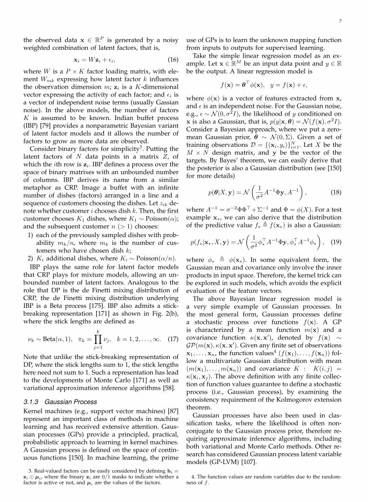
where W is a P ×K factor loading matrix, with ele-ment Wmk expressing how latent factor k influencesthe observation dimension m; zi is a K-dimensionalvector expressing the activity of each factor; and εi isa vector of independent noise terms (usually Gassiannoise). In the above models, the number of factorsK is assumed to be known. Indian buffet process(IBP) [79] provides a nonparametric Bayesian variantof latent factor models and it allows the number offactors to grow as more data are observed.

Consider binary factors for simplicity3. Putting thelatent factors of N data points in a matrix Z, ofwhich the ith row is zi. IBP defines a process over thespace of binary matrixes with an unbounded numberof columns. IBP derives its name from a similarmetaphor as CRP. Image a buffet with an infinitenumber of dishes (factors) arranged in a line and asequence of customers choosing the dishes. Let zik de-note whether customer i chooses dish k. Then, the firstcustomer chooses K1 dishes, where K1 ∼ Poisson(α);and the subsequent customer n (> 1) chooses:

1) each of the previously sampled dishes with prob-ability mk/n, where mk is the number of cus-tomers who have chosen dish k;

2) Ki additional dishes, where Ki ∼ Poisson(α/n).IBP plays the same role for latent factor models

that CRP plays for mixture models, allowing an un-bounded number of latent factors. Analogous to therole that DP is the de Finetti mixing distribution ofCRP, the de Finetti mixing distribution underlyingIBP is a Beta process [175]. IBP also admits a stick-breaking representation [171] as shown in Fig. 2(b),where the stick lengths are defined as

νk ∼ Beta(α, 1), πk =

k∏j=1

νj , k = 1, 2, . . . ,∞. (17)

Note that unlike the stick-breaking representation ofDP, where the stick lengths sum to 1, the stick lengthshere need not sum to 1. Such a representation has leadto the developments of Monte Carlo [171] as well asvariational approximation inference algorithms [58].

3.1.3 Gaussian ProcessKernel machines (e.g., support vector machines) [87]represent an important class of methods in machinelearning and has received extensive attention. Gaus-sian processes (GPs) provide a principled, practical,probabilistic approach to learning in kernel machines.A Gaussian process is defined on the space of contin-uous functions [150]. In machine learning, the prime

3. Real-valued factors can be easily considered by defining hi =zi µi, where the binary zi are 0/1 masks to indicate whether afactor is active or not, and µi are the values of the factors.

use of GPs is to learn the unknown mapping functionfrom inputs to outputs for supervised learning.

Take the simple linear regression model as an ex-ample. Let x ∈ RM be an input data point and y ∈ Rbe the output. A linear regression model is

f(x) = θ>φ(x), y = f(x) + ε,

where φ(x) is a vector of features extracted from x,and ε is an independent noise. For the Gaussian noise,e.g., ε ∼ N (0, σ2I), the likelihood of y conditioned onx is also a Gaussian, that is, p(y|x,θ) = N (f(x), σ2I).Consider a Bayesian approach, where we put a zero-mean Gaussian prior, θ ∼ N (0,Σ). Given a set oftraining observations D = (xi, yi)Ni=1. Let X be theM × N design matrix, and y be the vector of thetargets. By Bayes’ theorem, we can easily derive thatthe posterior is also a Gaussian distribution (see [150]for more details)

p(θ|X,y) = N(

1

σ2A−1Φy, A−1

), (18)

where A−1 = σ−2ΦΦ>+Σ−1 and Φ = φ(X). For a testexample x∗, we can also derive that the distributionof the predictive value f∗ , f(x∗) is also a Gaussian:

p(f∗|x∗, X,y) = N(

1

σ2φ>∗ A

−1Φy, φ>∗ A−1φ∗

), (19)

where φ∗ , φ(x∗). In some equivalent form, theGaussian mean and covariance only involve the innerproducts in input space. Therefore, the kernel trick canbe explored in such models, which avoids the explicitevaluation of the feature vectors.

The above Bayesian linear regression model isa very simple example of Gaussian processes. Inthe most general form, Gaussian processes definea stochastic process over functions f(x). A GPis characterized by a mean function m(x) and acovariance function κ(x,x′), denoted by f(x) ∼GP(m(x), κ(x,x′). Given any finite set of observationsx1, . . . ,xn, the function values4 (f(x1), . . . , f(xn)) fol-low a multivariate Gaussian distribution with mean(m(x1), . . . ,m(xn)) and covariance K : K(i, j) =κ(xi,xj). The above definition with any finite collec-tion of function values guarantee to define a stochasticprocess (i.e., Gaussian process), by examining theconsistency requirement of the Kolmogorov extensiontheorem.

Gaussian processes have also been used in clas-sification tasks, where the likelihood is often non-conjugate to the Gaussian process prior, therefore re-quiring approximate inference algorithms, includingboth variational and Monte Carlo methods. Other re-search has considered Gaussian process latent variablemodels (GP-LVM) [107].

4. The function values are random variables due to the random-ness of f .

8

3.1.4 Extensions

To meet the flexibility and adaptivity requirementsof big learning, many recent advances have beenmade on developing sophisticated NPB methods formodeling various types of data, including groupeddata, spatial data, time series, and networks.

Hierarchical models are natural tools to describegrouped data, e.g., documents from different sourcedomains. Hierarchical Dirichlet process (HDP) [172]and hierarchical Beta process [175] have been devel-oped, allowing an infinite number of latent compo-nents to be shared by multiple domains. The work [8]presents a cascading IBP (CIBP) to learn the topo-logical structure of multiple layers of latent features,including the number of layers, the number of hiddenunits at each layer, the connection structure betweenunits at neighboring layers, and the activation func-tion of hidden units. The recent work [52] presentsan extended CIBP process to generate connectionsbetween non-consecutive layers.

Another dimension of the extensions concerns mod-eling the dependencies between observations in a timeseries. For example, DP has been used to develop theinfinite hidden Markov models [23], which posit thesame sequential structure as in the hidden Markovmodels, but allowing an infinite number of latentclasses. In [172], it was shown that iHMM is a specialcase of HDP. The recent work [198] presents a max-margin training of iHMMs under the regularizedBayesian framework, as will be reviewed shortly.

Finally, for spatial data, modeling dependency be-tween nearby data points is important. Recent ex-tensions of Bayesian nonparametric methods includethe dependent Dirichlet process [120], spatial Dirichletprocess [59], distance dependent CRP [32], dependentIBP [188], and distance dependent IBP [70]. For net-work data analysis (e.g., social networks, biologicalnetworks, and citation networks), recent extensionsinclude the nonparametric Bayesian relational latentfeature models for link prediction [128], [200], whichadopt IBP to allow for an unbounded number of latentfeatures, and the nonparametric mixed membershipstochastic block models for community discovery [77],[98], which use HDP to allow mixed membership inan unbounded number of latent communities.

3.2 Regularized Bayesian Inference

Regularized Bayesian inference (RegBayes) [203] rep-resents one recent advance that extends the scope ofBayesian methods on incorporating rich side informa-tion. Recall that the classic Bayes’ theorem is equiv-alent to a variational optimization problem as in (2).RegBayes builds on this formulation and defines thegeneric optimization problem

minq(Θ)∈P

KL(q(Θ)‖p(Θ|D)) + c · Ω(q(Θ);D), (20)

where Ω(q(Θ);D) is the posterior regularization term;c is a nonnegative regularization parameter; andp(Θ|D) is the ordinary Bayesian posterior. Fig. 3 pro-vides a high-level comparison between RegBayes andBayes’ rule. Several questions need to be answered inorder to solve practical problems.

Q: How to define the posterior regularization?A: In general, posterior regularization can be any

informative constraints that are expected to regularizethe properties of the posterior distribution. It canbe defined as the large-margin constraints to enforcea good prediction accuracy [201], or the logic con-straints to incorporate expert knowledge [126], or thesparsity constraints [102].

Example 3: Max-margin LDA Following theparadigm of ordinary Bayes, a supervised topic modelis often defined by augmenting the likelihood model.For example, the supervised LDA (sLDA) [35] hasa similar structure as LDA (see Fig. 1(c)), but withan additional likelihood p(yd|zd,η) to describe labels.Such a design can lead to an imbalanced combinationof the word likelihood p(wd|zd,ψ) and the label likeli-hood because a document often has tens or hundredsof words while only one label. The imbalance problemcauses unsatisfactory prediction results [204].

To improve the discriminative power of supervisedtopic models, the max-margin MedLDA has beendeveloped, under the RegBayes framework. Considerbinary classification for simplicity. In this case, wehave Θ = θi, zi,ψk. Let f(η, zi) = η>zi be thediscriminant function5, where zi is the average topicassignments, with zki = 1

Li

∑j I(zij = k). The poste-

rior regularization can be defined in two ways:Averaging classifier: An averaging classifier makes

predictions using the expected discriminant function,that is, y(q) = sign(Eq[f(η, z)]). Let (x)+ = max(0, x).Then, the posterior regularization

ΩAvg(q(Θ);D) =N∑i=1

(1− yiEq[f(η, zi)])+

is an upper bound of the training error, therefore agood surrogate loss for learning. This strategy hasbeen adopted in MedLDA [201].

Gibbs classifier: A Gibbs classifier (or stochastic clas-sifier) randomly draws a sample (η, zd) from thetarget posterior q(Θ) and makes predictions using thelatent prediction rule, that is, y(η, zi) = signf(η, zi).Then, the posterior regularization is defined as

ΩGibbs(q(Θ);D) = Eq

[N∑i=1

(1− yif(η, zi))+

].

This strategy has been adopted to develop GibbsMedLDA [202].

The two strategies are closely related, e.g., wecan show that ΩGibbs(q(Θ)) is an upper bound of

5. We ignore the offset for simplicity.

9

prior distribution

likelihood model

posterior distribution

prior distribution

likelihood model

posterior distribution

posterior regularization

Bayes’ Rule Optimization

(a)

prior distribution

likelihood model

posterior distribution

prior distribution

likelihood model

posterior distribution

posterior regularization

Bayes’ Rule Optimization

(b)

Figure 3. (a) Bayesian inference with the Bayes’ rule; and (b) regularized Bayesian inference (RegBayes) whichsolves an optimization problem with a posterior regularization term to incorporate rich side information.

ΩAvg(q(Θ)). The formulation with a Gibbs classifiercan lead to a scalable Gibbs sampler by using dataaugmentation techniques [205]. If a logistic log-lossis adopted to define the posterior regularization, animproved sLDA model can be developed to addressthe imbalance issue and lead to significantly moreaccurate predictions [204].

Q: What is the relationship between prior, likeli-hood, and posterior regularization?

A: Though the three parts are closely connected,there are some key differences. First, prior is cho-sen before seeing data, while both likelihood andposterior regularization depend on the data. Second,different from the likelihood, which is restricted to bea normalized distribution, no constraints are imposedon the posterior regularization. Therefore, posteriorregularization is much more flexible than prior orlikelihood. In fact, it can be shown that (1) puttingconstraints on priors is a special case of posteriorregularization, where the regularization term doesnot depend on data; and (2) RegBayes can be moreflexible than standard Bayes’ rule, that is, there existssome RegBayes posterior distributions that are notachievable by the Bayes’ rule [203].

Q: How to solve the optimization problem?A: The posterior regularization term affects the

difficulty of solving problem (20). When the regular-ization term is a convex functional of q(Θ), whichis common in many applications such as the abovemax-margin formulations, the optimal solution can becharacterized in a general from via convex dualitytheory [203]. When the regularization term is non-convex, a generalized representation theorem can alsobe derived, but requires more effects on dealing withthe non-convexity [102].

4 SCALABLE ALGORITHMS

To deal with big data, the posterior inference algo-rithms should be scalable. Significant advances havebeen made in two aspects: (1) using random samplingto do stochastic or online Bayesian inference; and (2)using multi-core and multi-machine architectures todo parallel and distributed Bayesian inference.

4.1 Stochastic AlgorithmsIn Big Learning, the intriguing results of [38] suggestthat an algorithm as simple as stochastic gradient

descent (SGD) can be optimally efficient in terms of“number of bits learned per unit of computation”.For Bayesian models, both stochastic variational andstochastic Monte Carlo methods have been developedto explore the redundancy of data relative to a modelby subsampling data examples for every update andreasoning about the uncertainty created in this pro-cess [184]. We overview each type in turn.

4.1.1 Stochastic Variational MethodsAs we have stated in Section 2.3.1, variational meth-ods solve an optimization problem to find the bestapproximate distribution to the target posterior. Whenthe variational distribution is characterized in someparametric form, this problem can be solved withstochastic gradient descent (SGD) methods [40] or theadaptive SGD [60]. A SGD method randomly drawsa subset Bt and updates the variational parametersusing the estimated gradients, that is,

φt+1 ← φt + εt (∇φKL(q‖p0(θ))−∇φEq[log p(D|θ)]) ,

where the full data gradient is approximated as

∇φEq[log p(D|θ)] ≈ N

|Bt|∑i∈Bt

∇φEq[log p(xi|θ)], (21)

and εt is a learning rate. If the noisy gradient is anunbiased estimate of the true gradient, the procedureis guaranteed to approach the optimal solution whenthe learning rate is appropriately set [37].

For Bayesian latent variable models, we need to in-fer the latent variables when performing the updates.In general, we can group the latent variables intotwo categories — global variables and local variables.Global variables correspond to the model parametersθ (e.g., the topics ψ in LDA), while local variablesrepresent some hidden structures of the data (e.g., thetopic assignments z in an LDA with the topic mixingproportions collapsed out). Fig. 4 provides an illus-tration of such models and the stochastic variationalinference, which consists of three steps:

1) randomly draw a mini-batch Bt of data samples;2) infer the local latent variables for each data in Bt;3) update the global variables.However, the standard gradients over the param-

eters φ may not be the most informative direction(i.e., the steepest direction) to search for the distri-bution q. A better way is to use natural gradient [14],

10

i xi

global variables

local variables

sampling analysis model update

qt+1(µ)B t q¤(Ht)

draw a mini-batch

infer the hidden structure

update distribution of global variables

Figure ?: Graphical illustrations of: (a) the abstraction of models with latent structures; and (b) the procedure of BayesPA learning with latent structures.

(a) (b) Figure 4. (a) The general structure of Bayesian latent variable models, where hi denotes the local latent variablesfor each data i; (b) the process of stochastic variational inference, where the red arrows denote that in practicewe may need multiple iterations between “analysis” and “model update” to have fast convergence.

which is the steepest search direction in a Rieman-nian manifold space of probability distributions [86].To reduce the efforts on hand-tuning the learningrate, which often influences the performance much,the work [149] presents an adaptive learning ratewhile [165] adopts Bayesian optimization to searchfor good learning rates, both leading to faster con-vergence. By borrowing the gradient averaging ideasfrom stochastic optimization, [123] proposes to usesmoothed gradients in stochastic variational infer-ence to reduce the variance (by trading-off the bias).Stochastic variational inference methods have beenstudied for many Bayesian models, such as LDA andhierarchical Dirichlet process [86].

In many cases, the ELBO and its gradient may be in-tractable to compute due to the intractability of the ex-pectation over variational distributions. Two types ofmethods are commonly used to address this problem.First, another layer of variational bound is derivedby introducing additional variational parameters. Thishas been used in many examples, such as the logistic-normal topic models [34] and supervised LDA [35].For such methods, it is important to develop tightvariational bounds for specific models [124], whichis still an active area. Another type of methods is touse Monte Carlo estimates of the variational boundas well as its gradients. Recent work includes thestochastic approximation scheme with variance re-duction [141], [149] and the auto-encoding variationalBayes (AEVB) [99] that learns a neural network (a.k.arecognition model) to represent the variational distri-bution for continuous latent variables.

Consider the model with one layer of continuouslatent variables hi in Fig. 4 (a). Assume the varia-tional distribution qφ(Θ) = qφ(θ)

∏Ni=1 qφ(hi|xi). Let

Gφ(x,h,θ) = log p(h|θ) + log p(x|h,θ) − log qφ(h|x).The ELBO in Eq. (2) can be written as

L(φ;D) = Eq

[log p0(θ) +

∑i

Gφ(xi,hi,θ)− log qφ(θ)

].

By using the equality ∇φqφ(Θ) = qφ(Θ)∇φ log qφ(Θ),it can be shown that the gradient is

∇φL = Eq [(log p(Θ,D)− log qφ(Θ))∇φ log qφ(Θ)] .

A naive Monte Carlo estimate of the gradient is

∇φL ≈1

L

L∑l=1

[(log p(Θl,D)− log qφ(Θl))∇φ log qφ(Θl)

],

where Θl ∼ qφ(Θ). Note that the sampling and thegradient ∇φ log qφ(Θl) only depend on the variationaldistribution, not the underlying model. However, thevariance of such an estimate can be too large tobe useful. In practice, effective variance reductiontechniques are needed [141], [149].

For continuous h, a reparameterization of the sam-ples h ∼ qφ(h|x) can be derived using a differentiabletransformation gφ(ε,x) of a noise variable ε:

h = gφ(ε,x), where ε ∼ p(ε). (22)

This is known as non-centered parameterization (NCP)in statistics [142], while the original representationis known as centered parameterization (CP). A similarNCP reparameterization exists for the continuous θ:

θ = fφ(ζ), where ζ ∼ p(ζ). (23)

Given a minibatch of data points Bt, we de-fine Fφ(xi,hii∈Bt

,θ) = N|Bt|

∑i∈Bt

Gφ(xi,hi,θ) +

log p0(θ) − log qφ(θ). Then, the Monte Carlo estimateof the variational lower bound is

L(φ;D) ≈ 1

L

L∑l=1

Fφ

(xi, gφ(εl,xi)i∈Bt

, fφ(ζl)), (24)

where εl ∼ p(ε) and ζl ∼ p(ζ). This stochastic estimatecan be maximized via gradient ascent methods.

It has been analyzed that CP and NCP possesscomplimentary strengths [142], in the sense that NCPis likely to work when CP does not and conversely.An accompany paper [100] to AEVB analyzes theconditions for gradient-based samplers (e.g., HMC)whether NCP can be effective or ineffective in re-ducing posterior dependencies; and it suggests touse the interleaving strategy between centered andnon-centered parameterization as previously studiedin [195]. AEVB has been extended to learn deepgenerative models [152] using the similar reparam-eterization trick on continuous latent variables. How-ever, AEVB cannot be directly applied to deal withdiscrete variables. In contrast, the work [131] presentsa sophisticated method to reduce the variance of the

11

naive Monte Carlo estimate for deep autoregressivemodels; thus it is applicable to both continuous anddiscrete latent variables.

4.1.2 Stochastic Monte Carlo Methods

The existing stochastic Monte Carlo methods canbe generally grouped into three categories, namely,stochastic gradient-based methods, the methods usingapproximate MH test with randomly sampled mini-batches, and data augmentation.

Stochastic Gradient: The idea of using gradientinformation to improve the mixing rates has been sys-tematically studied in various MC methods, includingLangevin dynamics and Hamiltanian dynamics [136].For example, the Langevin dynamics is an MCMCmethod that produces samples from the posteriorby means of gradient updates plus Gaussian noise,resulting in a proposal distribution p(θt+1|θt) by thefollowing equation:

θt+1 = θt +εt2

(∇θ log p0(θ) +∇θ log p(D|θ)) + ζt, (25)

where ζt ∼ N (0, εtI) is an isotropic Gaussian noiseand log p(D|θ) =

∑i log p(xi|θ) is the log-likelihood of

the full data set. The mean of the proposal distributionis in the direction of increasing log posterior due tothe gradient, while the Gaussian noise will preventthe samples from collapsing to a single maximum.A Metropolis-Hastings correction step is required tocorrect for discretisation error [155].

The stochastic ideas have been successfully ex-plored in these methods to develop efficient stochasticMonte Carlo methods, including stochastic gradientLangevin dynamics (SGLD) [185] and stochastic gra-dient Hamiltonian dynamics (SGHD) [48]. For exam-ple, SGLD replaces the calculation of the gradientover the full data set, with a stochastic approximationbased on a subset of data. Let Bt be the subset ofdata points uniformly sampled from the full data setat iteration t. Then, the gradient is approximated as:

∇θ log p(D|θ) ≈ N

|Bt|∑i∈Bt

∇θ log p(xi|θ). (26)

Note that SGLD doesn’t use a MH correction step, ascalculating the acceptance probability requires use ofthe full data set. Convergence to the posterior is stillguaranteed if the step sizes are annealed to zero at acertain rate, as rigorously justified in [145], [173].

To further improve the mixing rates, the stochasticgradient Fisher scoring method [10] was developed,which represents an extension of the Fisher scoringmethod based on stochastic gradients [159] by incor-porating randomness in a subsampling process. Sim-ilarly, exploring the Riemannian manifold structureleads to the development of stochastic gradient Rie-mannian Langevin dynamics (SGRLD) [143], whichperforms SGLD on the probability simplex space.

Approximate MH Test: Another category ofstochastic Monte Carlo methods rely on approximateMH test using randomly sampled subset of datapoints, since an exact calculation of the MH testin Eq. (10) scales linearly to the data size, whichis prohibitive for large-scale data sets. For example,the work [101] presents an approximate MH rulevia sequential hypothesis testing, which allows us toaccept or reject samples with high confidence usingonly a fraction of the data required for the exact MHrule. The systematic bias and its tradeoff with variancewere theoretically analyzed. Specifically, it is based onthe observation that the MH test rule in Eq. (10) canbe equivalently written as follows:

1) Draw γ ∼ Uniform[0, 1] and compute:

µ0 =1

Nlog

[γp0(Θt)q(Θ

′|Θt)

p0(Θ′)q(Θt|Θ′)

]µ =

1

N

N∑i=1

`i, where `i = logp(xi|Θ′)p(xi|Θt)

;

2) If µ > µ0 set Θt+1 ← Θ′; otherwise Θt+1 ← Θt.Note that µ0 is independent of the data set, thus canbe easily calculated. This reformulation of the MHtest makes it very easy to frame it as a statisticalhypothesis test, that is, given µ0 and a set of samples`t1 , . . . , `tn drawn without replacement from thepopulation `1, . . . , `N, can we decide whether thepopulation mean µ is greater than or less than thethreshold µ0? Such a test can be done by increasingthe cardinality of the subset until a prescribed confi-dence level is reached. The MH test with approximateconfidence intervals can be combined with the abovestochastic gradient methods (e.g., SGLD) to correcttheir bias. The similar sequential testing ideas can beapplied to Gibbs sampling, as discussed in [101].

Under the similar setting of approximate MH testwith subsets of data, the work [21] derives a newstopping rule based on some concentration bounds(e.g., the empirical Bernstein bound [22]), which leadsto an adaptive sampling strategy with theoreticalguarantees on the total variational norm between theapproximate MH kernel and the target distribution ofMH applied to the full data set.

Data Augmentation: The work [121] presents aFirefly Monte Carlo (FlyMC) method, which is guar-anteed to converge to the true target posterior. FlyMCrelies on a novel data augmentation formulation [61].Specifically, let zi be a binary variable, indicatingwhether data i is active or not, and Bi(Θ) be astrictly positive lower bound of the ith likelihood:0 < Bi(Θ) < Li(Θ) , p(xi|Θ). Then, the targetposterior p(Θ|D) is the marginal of the completeposterior with the augmented variables Z = ziNi=1:

p(Θ,Z|D) ∝ p0(Θ)

N∏i=1

p(xi|Θ)p(zi|xi,Θ), (27)

12

where p(zi|xi,Θ) = (1 − γi)ziγ

(1−zi)i and γi =

Bi(Θ)/Li(Θ). Then, we can construct a Markov chainfor the complete posterior by alternating betweenupdates of Θ conditioned on Z, which can be donewith any conventional MCMC algorithm, and updatesof Z conditioned on Θ, which can also been efficientlydone as we only need to re-calculate the likelihoods ofthe data points with active z variables, thus effectivelyusing a random subset of data points in each iterationof the MC methods.

4.2 Streaming AlgorithmsWe can see that both (21) and (26) need to knowthe data size N , which renders them unsuitable forlearning with streaming data, where data comes insmall batches without an explicit bound on the totalnumber as times goes along, e.g., tracking an aircraftusing radar measurements. This conflicts with thesequential nature of the Bayesian updating procedure.Specifically, let Bt be the small batch at time t. Giventhe posterior at time t, pt(Θ) := p(Θ|B1, . . . , Bt), theposterior distribution at time t+ 1 is

pt+1(Θ) := p(Θ|B1, . . . , Bt+1) =pt(Θ)p(Bt+1|Θ)

p(B1, . . . , Bt+1). (28)

In other words, the posterior at time t is actually play-ing the role of a prior for the data at time t+1 for theBayesian updating. Under the variational formulationof Bayes’ rule, streaming RegBayes [163] can naturallybe defined as solving:

minq(Θ)∈P

KL(q(Θ)‖pt(Θ)) + c · Ω(q(Θ);Bt+1), (29)

whose streaming update rule can be derived via con-vex analysis under a quite general setting.

The sequential updating procedure is perfectly suit-able for online learning with data streams, where arevisit to each data point is not allowed. However,one challenge remains on evaluating the posteriors. Ifthe prior is conjugate to the likelihood model (e.g., alinear Gaussian state-space model) or the state spaceis discrete (e.g., hidden Markov models [148], [161]),then the sequential updating rule can be done ana-lytically, for example, Kalman filters [96]. In contrast,many complex Bayesian models (e.g., the modelsinvolving non-Gaussianity, non-linearity and high-dimensionality) do not have closed-form expressionof the posteriors. Therefore, it is computationally in-tractable to do the sequential update.

4.2.1 Streaming Variational MethodsVarious effects have been made to develop streamingvariational Bayesian (SVB) methods [42]. Specifically,let A be a variational algorithm that calculates theapproximate posterior q: q(Θ) = A(p(Θ);B). Then,setting q0(Θ) = p0(Θ), one way to recursively com-pute an approximation to the posterior is

p(Θ|B1, . . . , Bt+1) ≈ qt+1(Θ) = A(qt(Θ), Bt+1). (30)

Under the exponential family assumption of q, thestreaming update rule has some analytical form.

The streaming RegBayes [163] provides a Bayesiangeneralization of online passive-aggressive (PA) learn-ing [50], when the posterior regularization term isdefined via the max-margin principle. The resultingonline Bayesian passive-aggressive (BayesPA) learn-ing adopts a similar streaming variational updateto learn max-margin classifiers (e.g., SVMs) in thepresence of latent structures (e.g., latent topic repre-sentations). Compared to the ordinary PA, BayesPAis more flexible on modeling complex data. For ex-ample, BayesPA can discover latent structures via ahierarchical Bayesian treatment as well as allowing fornonparametric Bayesian inference to resolve the com-plexity of latent components (e.g., using a HDP topicmodel to resolve the unknown number of topics).

4.2.2 Streaming Monte Carlo MethodsSequential Monte Carlo (SMC) methods [15], [116],[19] provide simulation-based methods to approx-imate the posteriors for online Bayesian inference.SMC methods rely on resampling and propagatingsamples over time with a large number of particles.A standard SMC method would require the full datato be stored for expensive particle rejuvenation toprotect particles against degeneracy, leading to anincreased storage and processing bottleneck as moredata are accrued. For simple conjugate models, suchas linear Gaussian state-space models, efficient up-dating equations can be derived using methods likeKalman filters. For a broader class of models, assumeddensity filtering (ADF) [106], [140] was developedto extend the computational tractability. Basically,ADF approximates the posterior distribution witha simple conjugate family, leading to approximateonline posterior tracking. Recent improvements onSMC methods include the conditional density filtering(C-DF) method [81], which extends Gibbs samplingto streaming data. C-DF sequentially draws samplesfrom an approximate posterior distribution condi-tioned on surrogate conditional sufficient statistics,which are approximations to the conditional sufficientstatistics using sequential samples or point estimatesfor parameters along with the data. C-DF requiresonly data at the current time and produces a provablygood approximation to the target posterior.

4.3 Distributed AlgorithmsRecent progress has been made on both distributedvariational and distributed Monte Carlo methods.

4.3.1 Distributed Variational MethodsIf the variational distribution is in some paramet-ric family (e.g., the exponential family), the vari-ational problem can be solved with generic opti-mization methods. Therefore, the broad literature on

13

distributed optimization [39] provides rich tools fordistributed variational inference. However, the disad-vantage of a generic solver is that it may fail to explorethe structure of Bayesian inference.

First, many Bayesian models have a nature hier-archy, which encodes rich conditional independencestructures that can be explored for efficient algo-rithms, e.g., the distributed variational algorithm forLDA [197]. Second, the inference procedure withBayes’ rule is intrinsically parallelizable. Suppose thedata D is split into non-overlapping batches (oftencalled shards), B1, . . . , BM . Then, the Bayes posteriorp(Θ|D) =

p0(Θ)∏M

i=1 p(Bi|Θ)

p(D) can be expressed as

p(Θ|D) =1

C

M∏i=1

p0(Θ)1M p(Bi|Θ)

p(Bi)=

1

C

M∏i=1

p(Θ|Bi), (31)

where C = p(D)∏Mi=1 p(Bi)

. Now, the question is howto calculate the local posteriors (or subset posteri-ors) p(Θ|Bi) as well as the normalization factor. Thework [42] explores this idea and presents a distributedvariational Bayesian method, which approximates thelocal posterior with an algorithm A, that is, p(Θ|Bi) ≈A(p0(Θ)1/M , Bi

). Under the exponential family as-

sumption of the prior and the approximate localposteriors, the global posterior can be (approximately)calculated via density product. However, the paramet-ric assumptions may not be reasonable, and the mean-field assumptions can get the marginal distributionsright but not the joint distribution.

4.3.2 Distributed Monte Carlo MethodsFor MC methods, if independent samples can bedirectly drawn from the posterior or some pro-posals (e.g., using importance sampling), it will bestraightforward to parallelize, e.g., by running multi-ple independent samplers on separate machines andthen aggregating the samples [190]. We consider themore challenging cases, where directly sampling fromthe posterior is intractable and MCMC methods areamong the natural choices. There are two groups ofmethods. One is to run multiple MCMC chains inparallel, and the other is to parallelize a single MCMCchain. The “multiple-chain” parallelism is relativelystraightforward if each single chain can be efficientlycarried out and an appropriate combination strategyis adopted [67], [190]. However, in Big data applica-tions a single Markov chain itself is often prohibitivelyslow to converge, due to the massive data sizes orextremely high-dimensional sample spaces. Below, wefocus on the methods that parallelize a single Markovchain, under three major categories.

Blocking: Methods in this category let each com-puting unit (e.g., a CPU processor or a GPU core)to perform a part of the computation at each it-eration. For example, they independently evaluatethe likelihood for each shard across multiple units

and combine the local likelihoods with the prior ona master unit to get estimates of the global poste-rior [168]. Another example is that each computingunit is responsible for updating a part of the statespace [186]. These methods involve extensive commu-nications and being problem specific.

In these methods several computing units collab-orate to obtain a draw from the posterior. In orderto effectively split the likelihood evaluation or thestate space update over multiple computing units,it is important to explore the conditional indepen-dence (CI) structure of the model. Many hierarchicalBayesian models naturally have the CI structure (e.g.,topic models), while some other models need sometransformation to introduce CI structures that areappropriate for parallelization [189].

Divide-and-Conquer: Methods in this categoryavoid extensive communication among machines byrunning independent MCMC chains on each shardand aggregating samples drawn from local posteriorsvia a single communication. Aggregating the localsamples is the key step, with a lot of recent progress.For example, the consensus Monte Carlo [160] di-rectly combines local samples by a weighted average,which is valid under an implicit Gaussian assump-tion while lacking of guarantees for non-Gaussiancases; [137] approximates each local posterior witheither an explicit Gaussian or a Gaussian-kernel KDEso that combination follows an explicit density prod-uct; [181] builds upon the KDE idea one step furtherby representing the discrete KDE as a continuousWeierstrass transform; and [129] proposes to calcu-late the geometric median of local posteriors (or M-posterior), which is provably robust to the presenceof outliers. The M-posterior is approximately solvedby the Weiszfeld’s algorithm [26] by embedding thelocal posteriors in a reproducing kernel Hilbert space.

The potential drawback of these embarrassinglyparallel MCMC sampling is that if the local pos-teriors differ significantly, perhaps due to noise ornon-random partitioning of the dataset across nodes,the final combination stage can result in inaccurateglobal posterior. The recent work [192] presents a con-text aware distributed Bayesian posterior samplingmethod to improve inference quality. By allowingnodes to effectively and efficiently share informationwith each other, each node will eventually draw sam-ples from a more accurate approximate full posterior,and therefore no long needs any combination.

Prefetching: The idea of prefetching is to make useof parallel processing to calculate multiple likelihoodsahead of time, and only use the ones which areneeded. Consider a generic random-walk metropolis-Hastings algorithm at time t. The subsequent stepscan be represented by a binary tree, where at each iter-ation a single new proposal is drawn from a proposaldistribution and stochastically accepted or rejected.So, at time t+n the chain has 2n possible future states,

14

reject accept

reject acceptreject accept

Figure 5. The possible outcomes in two iterations of aMetropolis-Hastings sampler.

as illustrated in Fig. 5. The vanilla version of prefetch-ing speculatively evaluates all paths in this binarytree [41]. Since only one path of these will be taken,with M cores, this approach achieves a speedup oflog2M with respect to single core execution, ignoringcommunication overheads. More efficient prefetchingapproaches have been proposed in [17] and [167]by better guessing the probabilities of explorationof both the acceptance and the rejection branches ateach node. The recent work [20] presents a delayedacceptance strategy for MH testing, which can be usedto improve the efficiency of prefetching.

As a special type of MCMC, Gibbs sampling meth-ods naturally follow a blocking scheme by iterat-ing over some partition of the variables. The earlyasynchronous Gibbs sampler [68] is highly parallelby sampling all variables simultaneously on separateprocessors. However, the extreme parallelism comesat a cost, e.g., the sampler may not converge tothe correct stationary distribution in some cases [76].The work [76] develops various variable partitioningstrategies to achieve fast parallelization, while main-taining the convergence to the target posterior, andthe work [92] analyzes the convergence and correct-ness of the asynchronous Gibbs sampler (a.k.a, theHogwild parallel Gibbs sampler) for sampling fromGaussian distributions. Many other parallel Gibbssampling algorithms have been developed for specificmodels. For example, various distributed Gibbs sam-plers [138], [164], [9], [117], [46] have been developedfor the vanilla LDA, [47] develops a distributed Gibbssampler via data augmentation to learn large-scaletopic graphs with a logistic-normal topic model, andparallel algorithms for DP mixtures have been devel-oped by introducing auxiliary variables for additionalCI structures [189], while with the potential risk ofcausing extremely imbalanced partitions [65].

Note that the stochastic methods and distributedcomputing are not exclusive. Combing both oftenleads to more efficient solutions. For example, foroptimization methods, parallel SGD methods havebeen extensively studied [206], [139]. In particular,[139] presents a parallel SGD algorithm without locks,called Hogwild!, where multiple processors are al-lowed equal access to the shared memory and areable to update individual components of memory atwill. Such a scheme is particularly suitable for sparselearning problems. For Bayesian methods, the dis-

tributed stochastic gradient Langevin dynamics (D-SGLD) method has been developed in [11] and furtherimproved for topic models in [194].

5 TOOLS, SOFTWARE AND SYSTEMS

Though stochastic algorithms are easy to implement,distributed methods often need a careful design of thesystem architectures and programming libraries. Forsystem architectures, we may have a shared memorycomputer with many cores, a cluster with many ma-chines interconnected by network (either commodityor high-speed), or accelerating hardware like graph-ics processing units (GPUs) and field-programmablegate arrays (FPGAs). We now review the distributedprogramming frameworks suitable for various systemarchitectures and existing tools for Bayesian inference.

5.1 System PrimitivesEvery architecture has its low-level libraries, in whichthe parallel computing units (e.g., threads, machines,or GPU cores) are explicitly visible to the programmer.

Shared Memory Computer: A shared memorycomputer passes data from one CPU core to anotherby simply storing it into the main memory. Therefore,the communication latency is low. It is also easy toprogram and acquire. Meanwhile it is prevalent—itis the basic component of large distributed clustersand host of GPUs or other accelerating hardware.Due to these reasons, writing a multi-thread programis usually the first step towards large-scale learning.However, its drawbacks include limited memory/IOcapacity and bandwidth, and restricted scalability,which can be addressed by distributed clusters.

Programmers work with threads in a shared mem-ory setting. A threading library supports: 1) spawninga thread and wait it to complete; 2) synchronization:method to prevent conflict access of resources, suchas locks; 3) atomic: operations, such as increment thatcan be executed in parallel safely. Besides threads andlocks, there are alternative programming frameworks.For example, Scala uses actor, which responds to amessage that it receives; Go uses channel, which isa multi-provider, multi-consumer queue. There arealso libraries automating specific parallel pattern,e.g., OpenMP [6] supports parallel patterns like par-ralel for or reduction, and synchronization patternslike barrier; TBB [4] has pipeline, lightweight greenthreads and concurrent data structures. Choosingright programming models sometimes can simplifythe implementation.

Accelerating Hardware: GPUs are self-containedparallel computational devices that can be housedin desktop or laptop computers. A single GPU canprovide floating operations per second (FLOPS) per-formance as good as a small cluster. Yet compared toconventional multi-core processors, GPUs are cheap,easily accessible, easy to maintain, easy to code, and

15

dedicated local devices with low power consumption.GPUs follow a single instruction multiple data (SIMD)pattern, i.e., a single program will be executed onall cores given different data. This pattern is suitablefor many ML applications. However, GPUs may belimited due to: 1) small memory capacity; 2) restrictedSIMD programming model; and 3) high CPU-GPU orGPU-GPU communication latency.

Many Bayesian inference methods have been accel-erated with GPUs. For example, [168] adopts GPUs toparallelize the likelihood evaluation in MCMC; [110]provides GPU parallelization for population-basedMCMC methods [88] as well as SMC samplers [132];and [25] uses GPU computing to develop fast Hamil-tonian Monte Carlo methods. For variational Bayesianmethods, [193] demonstrates an example of usingGPUs to accelerate the collapsed variational Bayesianalgorithm for LDA. More recently, SaberLDA [114]implements a sparsity-aware sampling algorithm onGPU, which scales sub-linearly with the number oftopics. BIDMach [44] is a distributed GPU frameworkfor machine learning, In particular, BIDMach LDAwith a single GPU is able to learn faster than the state-of-the-art CPU based LDA implementation [9], whichuse 100 CPUs.

Finally, acceleration with other hardware (e.g., FP-GAs) has also been investigated [45].

Distributed Cluster: For distributed clusters, a low-level framework should allow users to do: 1) Commu-nication: sending and receiving data from/to anothermachine or a group of machines; 2) Synchronization:synchronize the processes; 3) Fault handling: decidewhat to do if a process/machine breaks down. Forexample, MPI provides a set of primitives includingsend, receive, broadcast and reduce for communication.MPI also provides synchronization operations, suchas barrier. MPI handles fault by simply terminatingall processes. MPI works on various network infras-tructures, such as ethernet or Infiniband. Besides MPI,there are other frameworks that support communi-cation, synchronization and fault handling, such as1) message queues, where processes can put andget messages from globally shared message queues;2) remote procedural calls (RPCs), where a processcan invoke a procedure in another process, passingits own data to that remote procedure, and finallyget execution results. MrBayes [156], [13] provides aMPI-based parallel algorithm for Metropolis-coupledMCMC for Bayesian phylogenetic inference.

Programming with system primitive libraries aremost flexible and lightweight. However for sophisti-cated applications, which may require asynchronousexecution, need to modify the global parameters whilerunning, or need many parallel execution blocks, itwould be painful and error prone to write the parallelcode using the low-level system primitives. Below, wereview some high-level distributed computing frame-works, which automatically execute the user declared

master

slave

map reduce

server

client

(a) (b) (c)

Figure 6. Various architectures: (a) MapRe-duce/Spark; (b) Pregel/GraphLab; (c) Parameterservers.

tasks on desired architectures. We refer the readers to[27] for more details on GPUs, MapReduce, and someother examples (e.g., parallel online learning).

5.2 MapReduce and SparkMapReduce [54] is a distributed computing frame-work for key-value stores. It reads key-value storesfrom disk, performs some transformations to thesekey-value stores in parallel, and writes the final re-sults to disk. A typical MapReduce cycle involves thesteps: (1) Spawn some workers on all machines; (2)Workers read input key-value pairs in parallel from adistributed file system; (3) Map: Pass each key-valuepair to a user defined function, which will generatesome intermediate key-value pairs; (4) According tothe key, hash the intermediate key-value pairs to allmachines, then merge key-value pairs that have thesame key, result with (key, list of values) pairs; (5)Reduce: In parallel, pass each (key, list of values) pairsto a user defined function, which will generate someoutput key-value pairs; and (6) Write output key-value pairs to the file system.

There are two user defined functions, mapper and re-ducer. For ML, a key-value store is often data samples,mapper is often used for computing latent variables,likelihoods or gradients for each data sample, andreducer is often used to aggregate the informationfrom each data sample, where the information can beused for estimating parameters or checking conver-gence. [49] discusses a number of ML algorithms onMapReduce, including linear regression, naive Bayes,neural networks, PCA, SVM, etc. Mahout [1] is a MLpackage built upon Hadoop, an open source imple-mentation of MapReduce. Mahout provides collabora-tive filtering, classification, clustering, dimensionalityreduction and topic modeling algorithms. [197] is aMapReduce based LDA. However, a major drawbackof MapReduce is that it needs to read the data fromdisk at every iteration. The overhead of reading databecomes dominant for many iterative ML algorithmsas well as interactive data analysis tools [196].

Spark [196] is another framework for distributedML methods that involve iterative jobs. The core ofSpark is resilient data sets (RDDs), which is essentiallya dataset distributed across machines. RDD can bestored either in memory or disk: Spark decides itautomatically, and users can provide hints to Sparkwhich to store in memory. This avoids reading the

16

dataset at every iteration. Users can perform paralleloperations to RDDs, which will transform a RDD toanother. Available parallel operations are like foreachand reduce. We can use foreach to do the computationfor each data, and use reduce to aggregate informa-tion from data. Because parallel operations are justa parallel version of the corresponding serial opera-tions, a Spark program looks almost identical to itsserial counterpart. Spark can outperform Hadoop foriterative ML jobs by 10x, and is able to interactivelyquery a 39GB dataset in 1 second [196].

5.3 Iterative Graph Computing

Both MapReduce and Spark have a star architecture asin Fig. 6 (a), where only master-slave communicationis permitted; they do not allow one key-value pairto interact with another, e.g., reading or modifyingthe value of another key-value pair. The interaction isnecessary for applications like PageRank, Gibbs sam-pling, and variational Bayes optimized by coordinatedescent, all of which require variables to get their ownvalues based on other related variables. Hence therecomes graph computing, where the computationaltask is defined by a sparse graph that specifies thedata dependency, as shown in Fig. 6 (b).

Pregel [122] is a bulk synchronous parallel (BSP)graph computing engine. The computation model isa sparse graph with data on vertices and edges, whereeach vertex receives all messages sent to it in thelast iteration; updates data on the vertex based onthe messages; and sends out messages along adjacentedges. For example, Gibbs sampling can be done eas-ily by sending the vertex statistics to adjacent verticesand then the conditional probability can be computed.GPS [158] is an open source implementation of Pregelwith new features (e.g., dynamic graph repartition).

GraphLab [119] is a more sophisticated graph com-puting engine that allows asynchronous executionand flexible scheduling. A GraphLab iteration picksup a vertex v in the task queue; and passes the vertexto a user defined function, which may modify thedata on the vertex, its adjacent edges and vertices,and finally may add its adjacent vertices to the taskqueue. Note that several nodes can be evaluated inparallel as long as they do not violate the consistencyguarantee which ensures that GraphLab is equiva-lent with some serial algorithm. It has been used toparallelize a number of ML tasks, including matrixfactorization, Gibbs sampling and Lasso [119]. [204]presents a distributed Gibbs sampler on GraphLabfor an improved sLDA model using RegBayes. Severalother graph computing engines have been developed.For example, GraphX [191] is an extension of Sparkfor graph computing; and GraphChi [104] is a diskbased version of GraphLab.

5.4 Parameter ServersAll the above frameworks restrict the communica-tion between workers. For example, MapReduce andSpark don’t allow communication between workers,while Pregel and GraphLab only allow vertices tocommunicate with adjacent nodes. On the other side,many ML methods follow a pattern that: (1) Dataare partitioned on many workers; (2) There are someshared global parameters (e.g., the model weights in agradient descent method or the topic-word count ma-trix in the collapsed Gibbs sampler for LDA [80]); and(3) Workers fetch data and update (parts of) globalparameters based on their local data (e.g., using thelocal gradients or local sufficient statistics). Though itis straightforward to implement on shared memorycomputers, it is rather difficult in a distributed set-ting. The goal of parameter servers is to provide adistributed data structure for parameters.

A parameter server is a key-value store (like ahash map), accessible for all workers. It supportsfor get and set (or update) for each entry. In adistributed setting, both server and client consist ofmany nodes (see Fig. 6 (c)). Memcached [3] is anin memory key-value store that provides get andset for arbitrary data. However it doesn’t have amechanism to resolve conflicts raised by concurrentaccess, e.g. concurrent writes for a single entry. Ap-plications like [164] require to lock the global entrywhile updating, which leads to suboptimal perfor-mance. Piccolo [147] addresses this by introducinguser-defined accumulations, which correctly addressconcurrent updates to the same key. Piccolo has aset of built-in user defined accumulations such assummation, multiplication, and min/max.

One important tradeoff made by parameter serversis that they sacrifice consistency for less latency—get may not return the most recent value, so thatit can return immediately without waiting for mostrecent updates to reach the server. While this im-proves the performance significantly, it can potentiallyslow down convergence due to outdated parame-ters. [85] proposed Stale Synchronous Parallel (SSP),where the staleness of parameters is bounded and thefastest worker can be ahead of the slowest one byno more than τ iterations, where τ can be tuned toget a fast convergence as well as low waiting time.Petuum [51] is a SSP based parameter server. [115]proposed communication-reducing improvements, in-cluding key caching, message compression and mes-sage filtering, and it also supports elastically addingand removing both server and worker nodes.

Parameter servers have been deployed in learningvery large-scale logistic regression [115], deep net-works [53], LDA [9], [112] and Lasso [51]. [115] learnsa 2000-topic LDA with 5 billion documents and 5million unique tokens on 6000 machines in 20 hours.Yahoo! LDA [9] has a parameter server designedspecifically for Bayesian latent variable models and

17

it is the fastest available LDA software. There are abunch of distributed topic modeling softwares basedon Yahoo! LDA, including [205] for MedLDA and [47]for correlated topic models.

5.5 Model Parallel InferenceMapReduce, Spark and Parameter servers take thedata-parallelism approach, where data are partitionedacross machines and computations are performed oneach node given a copy of the globally shared model.However, as the model size rapidly grows (i.e., thelarge M challenge), the models cannot fit in a singlecomputer’s memory. Model-parallelism addresses thischallenge by partitioning the model and storing a partof the model on each node. Then, partial updates(i.e., the updates of model parts) are carried out oneach node. Benefits of model-parallelism include largemodel sizes, flexibility to focus workers on fastest-converging parameters, and more accurate conver-gence because no delayed update is involved.

STRADS [111] provides primitives for model-parallelism and it handles the distributed storage ofmodel and data automatically. STRADS requires thata partial update could be computed using just themodel part together with data. Users writes schedulethat assigns model sets to workers, push that computesthe partial updates for model, pop that applies updatesto model. An automatic sync primitive will ensurethat users always get the latest model. As a concreteexample, [199] demonstrates a model parallel LDA,in which both data and model are partitioned byvocabulary. In each iteration, a worker only sampleslatent variables and updates the model related tothe vocabulary part assigned to it. The model thenrotates between workers, until a full cycle is com-pleted. Unlike data parallel LDA [164], [9], [138], thesampler always uses the latest models and no read-write lock is needed on models, thereby leading tofaster convergence than data-parallel LDAs.

Note that model-parallelism is not a replacementbut a complement of data-parallelism. For example,[182] showed a two layer LDA system, where layer1 is model-parallelism and layer 2 consists of sev-eral local model-parallelism clusters performing asyn-chronous updates on an globally distributed model.

6 CONCLUSIONS AND PERSPECTIVESWe present a survey of recent advances on big learn-ing with Bayesian methods, including Bayesian non-parametrics, regularized Bayesian inference, and scal-able inference algorithms and the systems based-onstochastic subsampling or distributed computing. Itis helpful to note that our review is not exhaustive.In fact, big learning has attracted intense interestwith active research spanning diverse fields, includingmachine learning, databases, parallel and distributedsystems, and programming languages.

As reviewed above, big learning with Bayesianmethods has achieved substantial progress. However,considerable challenges still remain. We briefly dis-cuss several directions that are of promise for futureinvestigation. First, Bayesian methods have the ad-vantage to incorporate prior knowledge for efficientlearning, especially for the scenarios where a largenumber of training data is lacking, and character-ize uncertainty. For instance, the recent work [105]demonstrates an example for the challenging task ofone-shot learning, which achieves human-level per-formance by encoding the domain knowledge as ahierarchical Bayesian model. In contrast, deep learn-ing methods [109] stand at the other end of thespectrum—they are often learned in an end-to-endmanner by feeding a large set of training data, andthey often do not represent the uncertainty in thestructure or parameters of the neural networks. Anatural and important question that remains under-addressed is how to conjoin the flexibility of deeplearning and the learning efficiency of Bayesian meth-ods for robust learning. Another related importantquestion is how to effectively collect domain knowl-edge and incorporate it into the modeling and in-ference process. The work [126] has demonstratedan example that selectively incorporates the noisyknowledge collected from crowds for robust Bayesianinference, but much more are left unexplored.

Second, one of the lessons we learn from big learn-ing is that the best predictive performance is oftenobtained by building a highly flexible model (e.g.,deep neural networks [109]). Although nonparametricBayesian techniques are powerful in theory to rep-resent flexible models and automatically infer theircomplexity from an unbounded space, there is still alarge gap in practice, with very few real applications.Most of the evaluations are proof-of-concepts by be-ing hindered on small-scale problems or those withrelatively simple structures. For example, althoughsome attempts have demonstrated that a cascade IBPcan be applied to infer the structure of a sparse deepbelief network [8], these results are preliminary andcan only learn toy network structures. It needs furtherstudy on how to learn the structure of a sophisticatednetwork with state-of-the-art performance. In orderto fill up the practical gap of nonparametric models,we need to develop the algorithms that are accurateand scalable as well as the theory of defining flexiblenonparametric processes that can properly considerthe rich structures in various domains.

Third, a more powerful way of composing Bayesianmodels is offered by probabilistic programming6,which uses general-purpose computer programs torepresent probabilistic models and automates the in-ference procedure by building a universal engine. Sev-eral probabilistic programming languages have been

6. http://probabilistic-programming.org

18

developed, including BUGS7, Stan8, BLOG9, Church10

and Infer.Net11. However, scalable inference is stilla considerable challenge for these languages. Theexisting platforms for Bayesian inference do not wellsupport the advanced deep models and the recentscalable algorithms in distributed/stochastic settings.They do not well support the accelerating hardware(e.g., GPUs and FPGAs) either. In fact, the exis-tence of user-friendly platforms (e.g., Tensorflow [7],Theano [174] and Caffe [91]) has significantly boostedthe applications of deep learning in industry. It will bevery useful to fill up this gap for Bayesian methods,which can allow for rapid prototyping and testing ofdifferent models, therefore motivating wider adoptionof Bayesian methods. Edward12 is a recent system thatbuilds on Tensorflow for scalable Bayesian inference,but much work needs to be done.

Finally, the current machine learning methods ingeneral still require considerable human expertise indevising appropriate features, priors, models, andalgorithms. Much work has to be done in order tomake ML more widely used and eventually become acommon part of our day to day tools in data sciences.Along this line, several promising projects have beenstarted. Google prediction API is one of the earliestefforts that try to make ML accessible for beginnersby providing easy-to-use service. Microsoft AzureMLtakes a similar approach by providing a visual in-terface to help design experiments. SystemML [75]provides an R-like declarative language to specify MLtasks based on MapReduce, and MLBase [103] furtherimproves it by providing learning-specific optimizerthat transforms a declarative task into a sophisticatedlearning plan. Finally, Automated Statistician (Auto-Stat) [118] aims to automate the process of statisticalmodeling, by using Bayesian model selection strate-gies to automatically choose good models/featuresand to interpret the results in easy-to-understandways, in terms of automatically generated reports.Though still at a very early stage, such efforts wouldhave a tremendous impact on the fields that currentlyrely on expert statisticians, ML researchers, and datascientists.

ACKNOWLEDGEMENTSThe work is supported by National 973 Projects(2013CB329403), NSF of China Projects (61322308,61332007), and Tsinghua Initiative Scientific ResearchProgram (20121088071).

REFERENCES[1] Apache mahout: https://mahout.apache.org/.

7. http://www.mrc-bsu.cam.ac.uk/software/bugs/8. http://mc-stan.org/9. https://bayesianlogic.github.io/10. https://projects.csail.mit.edu/church/wiki/Church11. http://research.microsoft.com/en-

us/um/cambridge/projects/infernet/12. http://edwardlib.org/

[2] http://lshtc.iit.demokritos.gr/.[3] http://memcached.org.[4] https://www.threadingbuildingblocks.org/.[5] http://www.image-net.org/about-overview.[6] http://www.openmp.org.[7] M. Abadi, A. Agarwal, P. Barham, E. Brevdo, Z. Chen,

C. Citro, G. S. Corrado, A. Davis, J. Dean, M. Devin,S. Ghemawat, I. Goodfellow, A. Harp, G. Irving, M. Is-ard, Y. Jia, R. Jozefowicz, L. Kaiser, M. Kudlur, J. Leven-berg, D. Mane, R. Monga, S. Moore, D. Murray, C. Olah,M. Schuster, J. Shlens, B. Steiner, I. Sutskever, K. Talwar,P. Tucker, V. Vanhoucke, V. Vasudevan, F. Viegas, O. Vinyals,P. Warden, M. Wattenberg, M. Wicke, Y. Yu, and X. Zheng.TensorFlow: Large-scale machine learning on heterogeneoussystems, 2015. Software available from tensorflow.org.

[8] R. Adams, H. Wallach, and Z. Ghahramani. Learning thestructure of deep sparse graphical models. In AISTATS, 2010.

[9] A. Ahmed, M. Aly, J. Gonzalez, S. Narayanamurthy, andA. Smola. Scalable inference in latent variable models. InWSDM, 2012.

[10] S. Ahn, A. Korattikara, and M. Welling. Bayesian posteriorsampling via stochastic gradient fisher scoring. In ICML,2012.

[11] S. Ahn, B. Shahbaba, and M. Welling. Distributed stochasticgradient MCMC. In ICML, 2014.

[12] J. Aitchison and S. M. Shen. Logistic-normal distributions:Some properties and uses. Biometrika, 67(2):261–272, 1980.

[13] G. Altekar, S. Dwarkadas, J. Huelsenbeck, and F. Ronquist.Parallel Metropolis coupled Markov chain Monte Carlo forBayesian phylogenetic inference. Bioinformatics, 20(3):407–415, 2004.

[14] S. Amari. Natural gradient works efficiently in learning.Neural Comput., 10:251–276, 1998.

[15] C. Andrieu, A. Doucet, and R. Holenstein. Particle Markovchain Monte Carlo methods. J. R. Stat. Soc., Ser B, 72(3):269–342, 2010.

[16] C. Andrieu, N. D. Freitas, A. Doucet, and M. I. Jordan.An introduction to MCMC for machine learning. MachineLearning, 50:5–43, 2003.

[17] E. Angelino, E. Kohler, A. Waterland, M. Seltzer, and R. P.Adams. Accelerating MCMC via parallel predictive prefetch-ing. arXiv:1403.7265, 2014.

[18] C. Antoniak. Mixture of Dirichlet process with applicationsto Bayesian nonparametric problems. Ann. Stats., (273):1152–1174, 1974.

[19] M. Arulampalam, S. Maskell, N. Gordon, and T. Clapp. Atutorial on particle filters for online nonlinear/non-gaussianBayesian tracking. IEEE Trans. Signal Process., 50(2):174–188,2002.

[20] M. Banterle, C. Grazian, and C. P. Robert. AcceleratingMetropolis-Hastings algorithms: Delayed acceptance withprefetching. arXiv:1406.2660, 2014.

[21] R. Bardenet, A. Doucet, and C. Holmes. Towards scalingup Markov chain Monte Carlo: an adaptive subsamplingapproach. In ICML, 2014.

[22] R. Bardenet and O.-A. Maillard. Concentration inequalitiesfor sampling without replacement. arXiv:1309.4029, 2013.

[23] M. Beal, Z. Ghahramani, and C. Rasmussen. The infinitehidden markov model. In NIPS, 2002.

[24] M. J. Beal. Variational algorithms for approximate Bayesianinference. PhD Thesis, University of Cambridge, 2003.

[25] A. L. Beam, S. K. Ghosh, and J. Doyle. Fast HamiltonianMonte Carlo using GPU computing. arXiv:1402.4089, 2014.

[26] A. Beck and S. Sabach. Weiszfelds method: Old and newresults. J. of Opt. Theory and Applications, 2014.

[27] R. Bekkerman, M. Bilenko, and J. Langford. Scaling upmachine learning: Parallel and distributed approaches. CambridgeUniversity Press, 2011.

[28] S. Bengio, J. Weston, and D. Grangier. Label embedding treesfor large multi-class tasks. In NIPS, 2010.

[29] Y. Bengio, A. Courville, and P. Vincent. RepresentationLearning: A Review and New Perspectives. IEEE Trans. onPAMI, 35(8):1798–1828, 2013.

[30] W. Bialek, I. Nemenman, and N. Tishby. Predictability,complexity and learning. Neural Comput., 13:2409–2463, 2001.

[31] C. M. Bishop. Pattern Recognition and Machine Learning.Springer, 2006.

19

[32] D. Blei and P. Frazier. Distance dependent Chinese restaurantprocesses. In ICML, 2010.

[33] D. Blei and M. Jordan. Variational inference for dirichletprocess mixtures. Bayesian Analysis, 1:121–144, 2006.

[34] D. Blei and J. Lafferty. Correlated topic models. In NIPS,2006.

[35] D. Blei and J. McAuliffe. Supervised topic models. In NIPS,2007.

[36] D. Blei, A. Ng, and M. I. Jordan. Latent Dirichlet Allocation.JMLR, (3):993–1022, 2003.

[37] L. Bottou. Online Algorithms and Stochastic Approximations.Online Learning and Neural Networks, Edited by DavidSaad, Cambridge University Press, Cambridge, UK, 1998.

[38] L. Bottou and O. Bousquet. The tradeoffs of large scalelearning. In NIPS, 2008.

[39] S. Boyd, N. Parikh, E. Chu, B. Peleato, and J. Eckstein. Dis-tributed Optimization and Statistical Learning via the AlternatingDirection Method of Multipliers, volume 3. Foundations andTrends in Machine Learning, 2011.

[40] S. Boyd and L. Vandenberghe. Convex Optimization. Cam-bridge University Press, 2004.

[41] A. Brockwell. Parallel Markov chain Monte Carlo simulationby pre-fetching. JCGS, 15(1):246–261, 2006.

[42] T. Broderick, N. Boyd, A. Wibisono, A. C. Wilson, and M. I.Jordan. Streaming variational Bayes. In NIPS, 2013.

[43] G. Brumfiel. High-energy physics: Down the petabyte high-way. Nature, 469:282–283, 2011.

[44] J. Canny and H. Zhao. Bidmach: Large-scale learning withzero memory allocation. In NIPS Big Learning Workshop, 2013.

[45] T. Chau, J. Targett, M. Wijeyasinghe, W. Luk, P. Cheung,B. Cope, A. Eele, and J. Maciejowski. Accelerating sequentialMonte Carlo method for real-time air traffic management.SIGARCH Computer Architecture News, 41(5):35–40, 2013.

[46] J. Chen, K. Li, J. Zhu, and W. Chen. Warplda: a cache efficiento (1) algorithm for latent dirichlet allocation. In VLDB, 2016.

[47] J. Chen, J. Zhu, Z. Wang, X. Zheng, and B. Zhang. Scalableinference for logistic-normal topic models. In NIPS, 2013.

[48] T. Chen, E. B. Fox, and C. Guestrin. Stochastic gradientHamiltonian Monte Carlo. In ICML, 2014.

[49] C. Chu, S. K. Kim, Y.-A. Lin, Y. Yu, G. Bradski, A. Y. Ng, andK. Olukotun. Map-reduce for machine learning on multicore.In NIPS, 2007.

[50] K. Crammer, O. Dekel, J. Keshet, S. Shalev-Shwartz, andY. Singer. Online passive-agressive algorithms. JMLR, (7):551–585, 2006.

[51] W. Dai, J. Wei, X. Zheng, J. K. Kim, S. Lee, J. Yin, Q. Ho,and E. Xing. Petuum: A framework for iterative-convergentdistributed ML. In arXiv:1312.7651, 2013.

[52] P. Dallaire, P. Giguere, and B. Chaib-draa. Learning thestructure of probabilistic graphical models with an extendedcascading Indian buffet process. In AAAI, 2014.

[53] J. Dean, G. Corrado, R. Monga, K. Chen, M. Devin, M. Mao,A. Senior, P. Tucker, K. Yang, Q. V. Le, et al. Large scaledistributed deep networks. In NIPS, 2012.

[54] J. Dean and S. Ghemawat. MapReduce: Simplified dataprocessing on large clusters. In OSDI, 2004.

[55] J. Deng, S. Satheesh, A. Berg, and L. Fei-Fei. Fast andbalanced: Efficient label tree learning for large scale objectrecognition. In NIPS, 2011.

[56] C. Doctorow. Big data: Welcome to the petacentre. Nature,455:16–21, 2008.

[57] S. Donnet, V. Rivoirard, J. Rousseau, and C. Scricciolo. Onconvergence rates of empirical Bayes procedures. In 47thScientific Meeting of the Italian Statistical Society, 2014.

[58] F. Doshi-Velez, K. Miller, J. V. Gael, and Y. W. Teh. Variationalinference for the Indian buffet process. In AISTATS, 2009.

[59] J. Duan, M. Guindani, and A. Gelfand. Generalized spatialDirichlet process models. Biometrika, 94(4), 2007.

[60] J. Duchi, E. Hazan, and Y. Singer. Adaptive subgradientmethods for online learning and stochastic optimization.JMLR, 12:2121–2159, 2011.

[61] D. V. Dyk and X. Meng. The art of data augmentation. JCGS,10(1):1–50, 2001.

[62] B. Efron. Bayes’ theorem in the 21st century. Science,340(6137):1177–1178, 2013.

[63] J. Fan, F. Han, and H. Liu. Challenges of big data analysis.National Science Review, 1(2):293–314, 2013.

[64] T. Ferguson. A Bayesian analysis of some nonparametricproblems. Ann. Stats., (1):209–230, 1973.

[65] Y. Gal and Z. Ghahramani. Pitfalls in the use of parallelinference for the Dirichlet process. In ICML, 2014.

[66] A. Gelman, J. Carlin, H. Stern, D. Dunson, A. Vehtari, andD. Rubin. Bayesian Data Analysis. Third Edition, Chapman &Hall/CRC Texts in Statistical Science), 2013.

[67] A. Gelman and D. Rubin. Inference from iterative simulationusing multiple simulations. Statist. Sci., 7(4):457–511, 1992.

[68] S. Geman and D. Geman. Stochastic relaxation, Gibbs distri-butions, and the Bayesian restoration of images. IEEE Trans.on PAMI, 6(1):721–741, 1984.

[69] E. I. George and D. P. Foster. Calibration and empirical Bayesvariable selection. Biometrika, 87(4):731–747, 2000.

[70] S. Gershman, P. Frazier, and D. Blei. Distance dependentinfinite latent feature models. arXiv:1110.5454, 2011.

[71] S. Gershmana and D. Blei. A tutorial on Bayesian nonpara-metric models. J. Math. Psychol., (56):1–12, 2012.

[72] C. J. Geyer and E. A. Thompson. Annealing Markov chainMonte Carlo with applications to ancestral inference. JASA,90(431):909–920, 1995.

[73] Z. Ghahramani. Bayesian nonparametrics and the probabilis-tic approach to modelling. Phil. Trans. of the Royal Society,2013.

[74] J. K. Ghosh and R. Ramamoorthi. Bayesian Nonparametrics.Springer, New York, NY, 2003.

[75] A. Ghoting, R. Krishnamurthy, E. Pednault, B. Reinwald,V. Sindhwani, and et al. SystemML: Declarative machinelearning on MapReduce. In ICDE, 2011.

[76] J. E. Gonzalez, Y. Low, A. Gretton, and C. Guestrin. ParallelGibbs sampling: From colored fields to thin junction trees. InAISTATS, 2011.

[77] P. Gopalan and D. Blei. Efficient discovery of overlappingcommunities in massive networks. PNAS, 110(36):14534–14539, 2013.

[78] A. Grelaud, C. P. Robert, J.-M. Marin, F. Rodolphe, and J.-F. Taly. Likelihood-free methods for model choice in Gibbsrandom fields. Bayesian Analysis, 4(2):317–336, 2009.

[79] T. Griffiths and Z. Ghahramani. Infinite latent feature modelsand the Indian buffet process. In NIPS, 2006.

[80] T. Griffiths and M. Steyvers. Finding scientific topics. PNAS,2004.

[81] R. Guhaniyogi, S. Qamar, and D. Dunson. Bayesian condi-tional density filtering for big data. arXiv:1401.3632, 2014.

[82] W. Hastings. Monte Carlo sampling methods using Markovchains and their applications. Biometrika, 57(1):97–109, 1970.

[83] G. Hinton, L. Deng, D. Yu, A. Mohamed, N. Jaitly, andetc. Deep neural networks for acoustic modeling in speechrecognition. IEEE Signal Process. Mag., 29(6):82–97, 2012.

[84] N. Hjort, C. Holmes, P. Muller, and S. Walker. BayesianNonparametrics: Principles and Practice. Cambridge UniversityPress, 2010.

[85] Q. Ho, J. Cipar, H. Cui, S. Lee, J. Kim, P. Gibbons, G. Gibson,G. Ganger, and E. Xing. More effective distributed ML via astale synchronous parallel parameter server. In NIPS, 2013.

[86] M. D. Hoffman, D. Blei, C. Wang, and J. Paisley. Stochasticvariational inference. JMLR, 14:1303–1347, 2013.

[87] T. Hofmann, B. Scholkopf, and A. J. Smola. Kernel methodsin machine learning. Ann. Statist., 36(3):1171–1220, 2008.

[88] A. Jasra, D. A. Stephens, and C. C. Holmes. On population-based simulation for static inference. Statistics and Computing,17(3):263–279, 2007.

[89] E. T. Jaynes. Prior probabilities. IEEE Trans. on Sys. Sci. andCybernetics, 4:227–241, 1968.

[90] H. Jeffreys. An invariant form for the prior probability inestimation problems. Proc. of the Royal Society of London. SeriesA, Mathematical and Physical Sciences, 186(1007):453–461, 1945.

[91] Y. Jia, E. Shelhamer, J. Donahue, S. Karayev, J. Long, R. Gir-shick, S. Guadarrama, and T. Darrell. Caffe: Convolu-tional architecture for fast feature embedding. arXiv preprintarXiv:1408.5093, 2014.

[92] M. J. Johnson, J. Saunderson, and A. S. Willsky. Analyzinghogwild parallel gaussian Gibbs sampling. In NIPS, 2013.

[93] M. Jordan. The era of big data. ISBA Bulletin, 18(2):1–3, 2011.[94] M. Jordan, Z. Ghahramani, T. Jaakkola, and L. Saul. An

introduction to variational methods for graphical models.MLJ, 37(2):183–233, 1999.

20

[95] J. B. Kadane and N. A. Lazar. Methods and criteria for modelselection. JASA, 99(465):279–290, 2004.

[96] R. E. Kalman. A new approach to linear filtering andprediction problems. J. Fluids Eng., 82(1):35–45, 1960.

[97] R. E. Kass and A. E. Raftery. Bayes factors. JASA, 90(430):773–795, 1995.

[98] D. I. Kim, P. Gopalan, D. M. Blei, and E. B. Sudderth. Effi-cient online inference for Bayesian nonparametric relationalmodels. In NIPS, 2013.

[99] D. Kingma and M. Welling. Auto-encoding variational bayes.In ICLR, 2014.

[100] D. Kingma and M. Welling. Efficient gradient-based inferencethrough transformations between Bayes nets and neural nets.In ICML, 2014.

[101] A. Korattikara, Y. Chen, and M. Welling. Austerity in MCMCland: Cutting the Metropolis-Hastings budget. In ICML, 2014.

[102] O. Koyejo and J. Ghosh. Constrained Bayesian inference forlow rank multitask learning. In UAI, 2013.

[103] T. Kraska, A. Talwalkar, J. Duchi, R. Griffith, M. Franklin, andM. Jordan. MLbase: A distributed machine-learning system.In CIDR, 2013.

[104] A. Kyrola, G. E. Blelloch, and C. Guestrin. GraphChi: Large-scale graph computation on just a PC. In OSDI, 2012.

[105] B. Lake, R. Salakhutdinov, and J. Tenenbaum. Human-levelconcept learning through probabilistic program induction.Science, 350(6266):1332–1338, 2015.

[106] S. L. Lauritzen. Propagation of probabilities, means andvariances in mixed graphical association models. JASA,87:1098–1108, 1992.

[107] N. Lawrence. Probabilistic non-linear principal componentanalysis with Gaussian process latent variable models. JMLR,(6):1783–1816, 2005.

[108] Q. Le, M. Ranzato, R. Monga, M. Devin, K. Chen, G. Corrado,J. Dean, and A. Ng. Building high-level features using largescale unsupervised learning. In ICML, 2012.

[109] Y. LeCun, Y. Bengio, and G. Hinton. Deep learning. Nature,521:436–444, 2015.

[110] A. Lee, C. Yau, M. B. Giles, A. Doucet, and C. C. Holmes.On the utility of graphics cards to perform massively par-allel simulation of advanced Monte Carlo methods. JCGS,19(4):769–789, 2010.

[111] S. Lee, J. K. Kim, X. Zheng, Q. Ho, G. Gibson, andE. Xing. Primitives for dynamic big model parallelism.arXiv:1406.4580, 2014.

[112] A. Q. Li, A. Ahmed, S. Ravi, and A. J. Smola. Reducing thesampling complexity of topic models. In SIGKDD, 2014.

[113] F.-F. Li and P. Perona. A bayesian hierarchical model forlearning natural scene categories. In CVPR, 2005.

[114] K. Li, J. Chen, W. Chen, and J. Zhu. Saberlda: Sparsity-aware learning of topic models on gpus. arXiv preprintarXiv:1610.02496, 2016.

[115] M. Li, D. Andersen, J. W. Park, A. Smola, A. Ahmed, V. Josi-fovski, J. Long, E. Shekita, and B.-Y. Su. Scaling distributedmachine learning with the parameter server. In OSDI, 2014.

[116] J. S. Liu and R. Chen. Sequential Monte Carlo methods fordynamic systems. JASA, 93(443):1032–1044, 1998.

[117] Z. Liu, Y. Zhang, E. Y. Chang, and M. Sun. PLDA+: Parallellatent Dirichlet allocation with data placement and pipelineprocessing. TIST, 2(3), 2011.

[118] J. Lloyd, D. Duvenaud, R. Grosse, J. Tenenbaum, andZ. Ghahramani. Automatic construction and natural lan-guage description of nonparametric regression models. InAAAI, 2014.

[119] Y. Low, J. Gonzalez, A. Kyrola, D. Bickson, C. Guestrin,and J. Hellerstein. Graphlab: A new framework for parallelmachine learning. In UAI, 2013.

[120] S. MacEachern. Dependent nonparametric processes. In ASAproceedings of the section on Bayesian statistical science, 1999.

[121] D. Maclaurin and R. P. Adams. Firefly Monte Carlo: ExactMCMC with subsets of data. In UAI, 2014.

[122] G. Malewicz, M. H. Austern, A. J. Bik, J. C. Dehnert, I. Horn,N. Leiser, and G. Czajkowski. Pregel: a system for large-scalegraph processing. In SIGMOD, 2010.

[123] S. Mandt and D. Blei. Smoothed gradients for stochasticvariational inference. arXiv:1406.3650, 2014.

[124] B. Marlin, E. Khan, and K. Murphy. Piecewise boundsfor estimating Bernoulli-logistic latent Gaussian models. InICML, 2011.

[125] J. D. McAuliffe, D. M. Blei, and M. I. Jordan. Nonparametricempirical Bayes for the Dirichlet process mixture model.Statistics and Computing, 16(1):5–14, 2006.

[126] S. Mei, J. Zhu, and X. Zhu. Robust RegBayes: Selec-tively incorporating first-order logic domain knowledge intoBayesian models. In ICML, 2014.

[127] N. Metropolis, A. Rosenbluth, M. Rosenbluth, A. Teller, andE. Teller. Equation of state calculations by fast computingmachines. J. Chem. Phys, 21(6):1087, 1953.

[128] K. Miller, T. Griffiths, and M. Jordan. Nonparametric latentfeature models for link prediction. In NIPS, 2009.

[129] S. Minsker, S. Srivastava, L. Lin, and D. B. Dunson. Scalableand robust Bayesian inference via the median posterior. InICML, 2014.

[130] T. Mitchell. Machine Learning. McGraw Hill, 1997.[131] A. Mnih and K. Gregor. Neural variational inference and

learning in belief networks. In ICML, 2014.[132] P. D. Moral, A. Doucet, and A. Jasra. Sequential Monte Carlo

samplers. J. R. Stat. Soc., Ser B, 68(3):411–436, 2006.[133] P. Muller and F. A. Quintana. Nonparametric Bayesian data

analysis. Statistical Science, 19(1):95–110, 2004.[134] R. Neal. Markov chain sampling methods for Dirichlet

process mixture models. JCGS, pages 249–265, 2000.[135] R. Neal. Slice sampling. Ann. Statist., 31(3):705–767, 2003.[136] R. Neal. MCMC using Hamiltonian Dynamics. Handbook of

Markov Chain Monte Carlo (S. Brooks, A. Gelman, G. Jones,and X.-L. Meng, eds.), Chapman & Hall / CRC Press, 2010.

[137] W. Neiswanger, C. Wang, and E. P. Xing. Asymptoticallyexact, embarrassingly parallel MCMC. In UAI, 2014.

[138] D. Newman, A. Asuncion, P. Smyth, and M. Welling. Dis-tributed inference for latent Dirichlet allocation. In NIPS,2007.

[139] F. Niu, B. Recht, C. Re, and S. J. Wright. Hogwild: A lock-free approach to parallelizing stochastic gradient descent. InNIPS, 2011.

[140] M. Opper. A Bayesian Approach to Online Learning. OnlineLearning in Neural Networks, Cambridge University, 1999.

[141] J. Paisley, D. M. Blei, and M. I. Jordan. Variational Bayesianinference with stochastic search. In ICML, 2012.

[142] O. Papaspiliopoulos, G. O. Roberts, and M. Skold. A generalframework for the parametrization of hierarchical models.Statistical Science, 22(1):59–73, 2007.

[143] S. Patterson and Y. W. Teh. Stochastic gradient RiemannianLangevin dynamics on the probability simplex. In NIPS, 2013.

[144] S. Petrone, J. Rousseau, and C. Scricciolo. Bayes and empiricalBayes: do they merge? Biometrika, pages 1–18, 2014.

[145] N. Pillai and A. Smith. Ergodicity of approximate MCMCchains with applications to large data sets. arXiv:1405.0182,2014.

[146] J. Pitman. Combinatorial stochastic processes. Technical ReportNo. 621. Department of Statistics, UC, Berkeley, 2002.

[147] R. Power and J. Li. Piccolo: Building fast, distributed pro-grams with partitioned tables. In OSDI, 2010.

[148] L. R. Rabiner. A tutorial on hidden Markov models andselected applications in speech recognition. Proc. of the IEEE,77(2):257–286, 1989.

[149] R. Ranganath, C. Wang, D. Blei, and E. Xing. An adaptivelearning rate for stochastic variational inference. In ICML,2013.

[150] C. E. Rasmussen and C. K. I. Williams. Gaussian Processes forMachine Learning. The MIT Press, 2006.

[151] O. Reichman, M. Jones, and M. Schildhauer. Challenges andopportunities of open data in ecology. Science, 331(6018):703–705, 2011.

[152] D. J. Rezende, S. Mohamed, and D. Wierstra. Stochastic back-propagation and approximate inference in deep generativemodels. In ICML, 2014.

[153] C. Robert and G. Casella. Monte Carlo Statistical Methods.Springer, 2005.

[154] C. P. Robert, J.-M. Cornuet, J.-M. Marin, and N. S. Pillai. Lackof confidence in approximate Bayesian computation modelchoice. PNAS, 108(37):15112–15117, 2011.

21

[155] G. Roberts and O. Strame. Langevin diffusions andMetropolis-Hastings algorithms. Methodology and Computingin Applied Probability, 4:337–357, 2002.

[156] F. Ronquist and J. Huelsenbeck. MrBayes: Bayesian inferenceof phylogenetic trees. Bioinformatics, 19(12):1572–1574, 2003.

[157] R. Salakhutdinov. Learning deep generative models. PhDThesis, University of Toronto, 2009.

[158] S. Salihoglu and J. Widom. GPS: A graph processing system.In SSDBM, 2013.

[159] N. Schraudolph, J. Yu, and S. Gunter. A stochastic Quasi-Newton method for online convex optimization. In AISTATS,2007.

[160] S. Scott, A. Blocker, F. Bonassi, H. Chipman, E. George, andR. McCulloch. Bayes and big data: The consensus MonteCarlo algorithm. EFaB Bayes 250 Workshop, 16, 2013.

[161] S. L. Scott. Bayesian methods for hidden Markov models.JASA, 97(457):337–351, 2002.

[162] J. Sethuraman. A constructive definition of dirichlet priors.Statistica Sinica, (4):639–650, 1994.

[163] T. Shi and J. Zhu. Online Bayesian passive-aggressive learn-ing. In ICML, 2014.

[164] A. Smola and S. Narayanamurthy. An architecture for paralleltopic models. VLDB, 2010.

[165] J. Snoek, H. Larochelle, and R. P. Adams. Practical Bayesianoptimization of machine learning algorithms. In NIPS, 2012.

[166] N. Srivastava, G. Hinton, A. Krizhevsky, I. Sutskever, andR. Salakhutdinov. Dropout: A simple way to prevent neuralnetworks from overfitting. JMLR, 15:1929–1958, 2014.

[167] I. Strid. Efficient parallelisation of Metropolis-Hastings algo-rithms using a prefetching approach. Computational Statisticsand Data Analysis, 54:2814–2835, 2010.

[168] M. Suchard, Q. Wang, C. Chan, J. Frelinger, A. Cron, andM. West. Understanding GPU programming for statisticalcomputation: Studies in massively parallel massive mixtures.JCGS, 19(2):419–438, 2010.

[169] M. Tan, I. Tsang, and L. Wang. Towards ultrahigh dimen-sional feature selection for big data. JMLR, (15):1371–1429,2014.

[170] M. Tanner and W. Wong. The calculation of posterior distri-butions by data augmentation. JASA, 82(398):528–540, 1987.

[171] Y. W. Teh, D. Gorur, and Z. Ghahramani. Stick-breakingconstruction for the Indian buffet process. In AISTATS, 2007.

[172] Y. W. Teh, M. I. Jordan, M. J. Beal, and D. M. Blei. HierarchicalDirichlet processes. JASA, 101(476):1566–1581, 2006.

[173] Y. W. Teh, A. Thiey, and S. Vollmer. Consistency andfluctuations for stochastic gradient Langevin dynamics.arXiv:1409.0578, 2014.

[174] Theano Development Team. Theano: A Python frameworkfor fast computation of mathematical expressions. arXiv e-prints, abs/1605.02688, May 2016.

[175] R. Thibaux and M. I. Jordan. Hierarchical Beta processes andthe Indian buffet process. In AISTATS, 2007.

[176] B. M. Turnera and T. V. Zandtb. A tutorial on approximateBayesian computation. J. Math. Psychol., 56(2):69–85, 2012.

[177] D. van Dyk and T. Park. Partially collapsed Gibbs samplers:Theory and methods. JASA, 103(482):790–796, 2008.

[178] P. Vincent, H. Larochelle, Y. Bengio, and P.-A. Manzagol.Extracting and composing robust features with denoisingautoencoders. In ICML, 2008.

[179] M. Wainwright and M. Jordan. Graphical models, exponen-tial families, and variational inference. Foundations and Trendsin Machine Learning, 1(1–2):1–305, 2008.

[180] S. G. Walker. Sampling the Dirichlet mixture model withslices. Commun Stat - Simul and Comput, 36:45–54, 2007.

[181] X. Wang and D. B. Dunson. Parallelizing MCMC via Weier-strass sampler. arXiv:1312.4605, 2013.

[182] Y. Wang, X. Zhao, Z. Sun, H. Yan, L. Wang, Z. Jin, L. Wang,Y. Gao, J. Zeng, Q. Yang, et al. Towards topic modeling forbig data. arXiv:1405.4402, 2014.

[183] K. Weinberger, A. Dasgupta, J. Langford, A. Smola, and J. At-tenberg. Feature hashing for large scale multitask learning.In ICML, 2009.

[184] M. Welling. Exploiting the statistics of learning and inference.In NIPS workshop on ”Probabilistic Models for Big Data”, 2013.

[185] M. Welling and Y. W. Teh. Bayesian learning via stochasticgradient Langevin dynamics. In ICML, 2011.

[186] D. Wilkinson. Parallel Bayesian computation. Handbook ofParallel Computing and Statistics, Chapter 18, 2004.

[187] P. M. Williams. Bayesian conditionalisation and the principleof minimum information. The British Journal for the Philosophyof Science, 31(2), 1980.

[188] S. Williamson, P. Orbanz, and Z. Ghahramani. DependentIndian buffet processes. In AISTATS, 2010.

[189] S. A. Williamson, A. Dubey, and E. P. Xing. Parallel Markovchain Monte Carlo for nonparametric mixture models. InICML, 2013.

[190] X.-L. Wu, C. Sun, T. Beissinger, G. Rosa, K. Weigel, N. Gatti,and D. Gianola. Parallel Markov chain Monte Carlo -bridging the gap to high-performance Bayesian computationin animal breeding and genetics. Genetics Seletion Evolution,44(1):29–46, 2012.

[191] R. S. Xin, J. E. Gonzalez, M. J. Franklin, and I. Stoica. Graphx:A resilient distributed graph system on spark. In Workshopon Graph Data Management Experiences and Systems, 2013.

[192] M. Xu, B. Lakshminarayanan, Y. Teh, J. Zhu, and B. Zhang.Distributed Bayesian posterior sampling via moment sharing.In NIPS, 2014.

[193] F. Yan, N. Xu, and A. Qi. Parallel inference for latent Dirichletallocation on graphics processing units. In NIPS, 2009.

[194] Y. Yang, J. Chen, and J. Zhu. Distributing the stochasticgradient sampler for large-scale lda. In KDD, 2016.

[195] Y. Yu and X.-L. Meng. To center or not to center: That is notthe question–an ancillarity–sufficiency interweaving strategy(asis) for boosting mcmc efficiency. JCGS, 20(3):531–570, 2011.

[196] M. Zaharia, M. Chowdhury, M. J. Franklin, S. Shenker, andI. Stoica. Spark: cluster computing with working sets. In HotTopics in Cloud Computing, 2010.

[197] K. Zhai, J. Boyd-Graber, N. Asadi, and M. L. Alkhouja. Mr.LDA: a flexible large scale topic modeling package usingvariational inference in MapReduce. In WWW, 2012.

[198] A. Zhang, J. Zhu, and B. Zhang. Max-margin infinite hiddenMarkov models. In ICML, 2014.

[199] X. Zheng, J. K. Kim, Q. Ho, and E. Xing. Model-parallelinference for big topic models. arXiv:1411.2305, 2014.

[200] J. Zhu. Max-margin nonparametric latent feature models forlink prediction. In ICML, 2012.

[201] J. Zhu, A. Ahmed, and E. Xing. MedLDA: maximum marginsupervised topic models. JMLR, (13):2237–2278, 2012.

[202] J. Zhu, N. Chen, H. Perkins, and B. Zhang. Gibbs max-margintopic models with fast sampling algorithms. In ICML, 2013.

[203] J. Zhu, N. Chen, and E. Xing. Bayesian inference withposterior regularization and applications to infinite latentSVMs. JMLR, 15:1799–1847, 2014.

[204] J. Zhu, X. Zheng, and B. Zhang. Improved Bayesian logisticsupervised topic models with data augmentation. In ACL,2013.

[205] J. Zhu, X. Zheng, L. Zhou, and B. Zhang. Scalable inferencein max-margin supervised topic models. In SIGKDD, 2013.

[206] M. A. Zinkevich, M. Weimer, A. Smola, and L. Li. Parallelizedstochastic gradient descent. In NIPS, 2010.