bifurcation control for a class of lorenz …pyu/pub/preprints/yl_ijbc2011.pdf · october 1, 2011...

October 1, 2011 12:9 WSPC/S0218-1274 03000

International Journal of Bifurcation and Chaos, Vol. 21, No. 9 (2011) 2647–2664c© World Scientific Publishing CompanyDOI: 10.1142/S0218127411030003

BIFURCATION CONTROL FOR A CLASSOF LORENZ-LIKE SYSTEMS

PEI YU∗Department of Applied Mathematics,

The University of Western Ontario London,Ontario, Canada N6A 5B7

[email protected]

JINHU LULSC, ISS, Academy of Mathematics and Systems Science,

Chinese Academy of Sciences, Beijing,100080, P. R. China

School of Electrical and Computer Engineering,RMIT University, Melbourne VIC 3001, Australia

Received August 15, 2010

In this paper, a control method developed earlier is employed to consider controlling bifurcationsin a class of Lorenz-like systems. Particular attention is focused on Hopf bifurcation control vialinear and nonlinear stability analyses. The Lorenz system, Chen system and Lu system arestudied in detail. Simple feedback controls are designed for controlling the stability of equilibriumsolutions, limit cycles and chaotic motions. All formulas are derived in general forms includingthe system parameters. Computer simulation results are presented to confirm the analyticalpredictions.

Keywords : Lorenz-like systems; bifurcation control; feedback controller; limit cycles; chaos.

1. Introduction

Bifurcation and chaos control has been exten-sively studied in the past three decades, and manymethodologies have been developed to solve phys-ical and engineering problems (e.g. see [Abed &Fu, 1987; Nayfeh et al., 1996; Yu & Huseyin,1988; Laufenberg et al., 1997; Wang & Abed, 1995;Ono et al., 1998; Berns et al., 2000; Chen et al.,2000; Kang & Krener, 2000; Chen et al., 2001;Lu et al., 2002a; Lu et al., 2002b; Chen & Lu,2003; Lu & Lu, 2003; Yu & Chen, 2004]). In gen-eral, the aim of bifurcation control is to designa controller such that the bifurcation property

of a nonlinear system undergoing bifurcation canbe changed to achieve certain desirable dynamicalbehavior, such as changing stability of equilibriumsolutions, making a Hopf bifurcation from subcrit-ical to supercritical, eliminating chaotic motions,etc. Anti-bifurcation control and chaotification, onthe other hand, are to purposefully create bifur-cation or chaos to satisfy a particular purpose ofdesign.

In this paper, our attention is focused onbifurcation control using nonlinear state feedback.A previously developed explicit formula [Yu &Chen, 2004] will be applied to consider a class

∗Author for correspondence

2647

Int.

J. B

ifur

catio

n C

haos

201

1.21

:264

7-26

64. D

ownl

oade

d fr

om w

ww

.wor

ldsc

ient

ific

.com

by U

NIV

ER

SIT

Y O

F W

EST

ER

N O

NT

AR

IO W

EST

ER

N L

IBR

AR

IES

on 0

7/25

/12.

For

per

sona

l use

onl

y.

http://dx.doi.org/10.1142/S0218127411030003

October 1, 2011 12:9 WSPC/S0218-1274 03000

2648 P. Yu & J. Lu

of Lorenz-like systems, including the Lorenz sys-tem, Chen system and Lu system. This formula isgiven in the form of polynomials, and keeps theequilibria of the original system unchanged. Thismethod has been used to study a simple Lorenz sys-tem (with only two independent parameters) andRossler system [Yu & Chen, 2004] where explicitcontrol designs are provided to show the applicabil-ity of the theory. To be more specific, consider thefollowing general nonlinear system:

x = f(x,µ), x ∈ Rn, µ ∈ Rm, f : Rn+m → Rn,

(1)

where the dot denotes differentiation with respectto time t,x is an n-dimensional state vector and µ isan m-dimensional parameter vector, which containsbifurcation parameters and control parameters. Thefunction f is assumed analytic with respect to bothx and µ.

Usually, the first step in the study of system (1)is to find its equilibrium solutions, which canbe solved from the nonlinear algebraic equationf(x,µ) = 0, usually yielding multiple solutions. Letx∗(µ) denote an equilibrium solution of the system,i.e. f(x∗(µ),µ) ≡ 0 for any value of µ. Further,suppose that the Jacobian of the system evaluatedat the equilibrium solution x∗(µ) has eigenvalues,λ1(µ), λ2(µ), . . . , λn(µ), which may be real or com-plex. Assume that when µ is varied, the real partof some eigenvalues becomes zero at the criticalpoint µ = µ∗, leading to certain type of bifurcation,such as Hopf bifurcation, Hopf-zero bifurcation,etc.

The goal of bifurcation control here is to designa controller, given by

u = u(x;µ), (2)

such that the original equilibrium solution x∗ isunchanged, but the bifurcation point (x∗,µ∗) ismoved to a new position, (x∗, µ), with µ �= µ.Therefore, a necessary condition for the controller is

u(x∗;µ) = 0, (3)

for all values of µ, in order not to change the origi-nal equilibrium solution x∗. More precisely, supposesystem (1) has k equilibria, given by

x∗i (µ) = (x∗

1i(µ), x∗2i(µ), . . . , x∗

ni(µ)),

i = 1, 2, . . . , k, (4)

satisfying f(x∗i (µ),µ) ≡ 0 for i = 1, 2, . . . , k.

The general nonlinear state feedback control (2) is

applied to system (1) to obtain a closed-loop controlsystem:

x = f(x,µ) + u(x,µ) ≡ F(x,µ). (5)

In order for the controlled system (5) to keep allthe original k equilibria unchanged under the con-trol u, it requires that the following conditions besatisfied:

u(x∗i ,µ) ≡ (u1, u2, . . . , un)T = 0 (6)

for i = 1, 2, . . . , k.A control law given in general polynomial func-

tion, satisfying condition (6), has been proposed[Yu & Chen, 2004]:

uq(x,x∗1,x

∗2, . . . ,x

∗k,µ)

=n∑

i=1

Aqi

k∏j=1

(xi − x∗ij)

+n∑

i=1

k∑j=1

Bqij (xi − x∗ij)

k∏p=1

(xi − x∗ip)

+n∑

i=1

k∑j=1

Cqij(xi − x∗ij)

2k∏

p=1

(xi − x∗ip)

+n∑

i=1

k∑j=1

Dqij(xi − x∗ij)

2k∏

p=1

(xi − x∗ip)

2 + · · ·

(q = 1, 2, . . . , n).(7)

It is easy to verify that uq(x∗i ,x

∗1,x

∗2, . . . ,x

∗k,µ) = 0

for i = 1, 2, . . . , k. It should be noted that althoughthe formula (7) contains linear terms, purely linearfeedback controls are not used since they only keepone of the equilibria unchanged.

Usually, terms given in Eq. (7) up to Dqij areenough for controlling a bifurcation if the singu-larity of the system is not highly degenerate. Thecoefficients Aqi, Bqij , Cqij and Dqij , which may befunctions of µ, are determined from the stabilityof an equilibrium under consideration and that ofthe associated bifurcation solutions. More precisely,linear terms are determined by requiring the shiftof an existing bifurcation (e.g. delaying an exist-ing Hopf bifurcation). The nonlinear terms, on theother hand, can be used to change the stability ofan existing bifurcation or create a new bifurcation(e.g. changing an existing subcritical Hopf bifurca-tion to supercritical). Note that not just Aqi terms

Int.

J. B

ifur

catio

n C

haos

201

1.21

:264

7-26

64. D

ownl

oade

d fr

om w

ww

.wor

ldsc

ient

ific

.com

by U

NIV

ER

SIT

Y O

F W

EST

ER

N O

NT

AR

IO W

EST

ER

N L

IBR

AR

IES

on 0

7/25

/12.

For

per

sona

l use

onl

y.

October 1, 2011 12:9 WSPC/S0218-1274 03000

Bifurcation Control for a Class of Lorenz-like Systems 2649

may involve linear terms; Bqij terms, etc. may alsocontain linear terms.

Note that it is not necessary to take all thecomponents uq, i = 1, 2, . . . , n, in the control. Inmost cases, using fewer components or just one com-ponent may be enough to satisfy the predesignedcontrol objectives. It is preferable to have a sim-plest possible design for engineering applications.For example, if x∗

i1 = x∗i2 = · · · = x∗

ik for some i,then one only needs to use these terms and omitthe remaining terms in the control law. Moreover,lower-order terms related to these equilibrium com-ponents can be added. In fact, although the for-mula (7) looks complicated, in application manycoefficients therein will be zero, as demonstrated inSecs. 3–5.

Stabilization of chaotic systems usually employLyapunov function to reach global stability, and lin-ear feedback controls may be used. However, sucha linear control does not keep all the equilibria ofthe system unchanged, but only stabilizes one ofthem. The Hopf bifurcation control studied in thispaper guarantees all the equilibria of the system iskept unchanged, though the stability is usually notglobal.

In the next section, the general strategy of Hopfbifurcation control is discussed. Section 3 is devotedto study bifurcation control of the Lorenz system,and Secs. 4 and 5, to consider the Chen and Lusystems, respectively. Finally, concluding remarksare given in Sec. 6.

2. A Class of Lorenz-like Systemsand Hopf Bifurcation Control

In this paper, we consider a class of Lorenz-likesystems, which has rich complex dynamical behav-ior, including bifurcations to equilibrium solutions,periodic and quasi-periodic solutions and chaoticmotions. This class of Lorenz-like systems can begenerally described by

x = a(y − x),

y = dx + cy − xz, (8)

z = −bz + xy,

where a, b, c and d are real parameters. System (8)is the Lorenz system when c = −1; the Chen systemwhen d = c−a; and the Lu system when d = 0. Thetypical chaotic attractors for the three systems areshown in Fig. 1. It should be noted that the classof Lorenz-like systems, described by (8) are more

-25 -20 -15 -10 -5 0 5 10 15 20 25 -30-20

-100

10 20

30

0

10

20

30

40

50

z

x

y

z

(a)

-25 -20 -15 -10 -5 0 5 10 15 20 25 -30-20

-100

10 20

30

0

10

20

30

40

50

z

x

y

z

(b)

-25 -20 -15 -10 -5 0 5 10 15 20 25 -30-20

-100

10 20

30

0

10

20

30

40

50

z

x

y

z

(c)

Fig. 1. Simulated trajectories for system (8); (a) the Lorenzattractor when a = 10, b = 8/3, c = −1, d = 28; (b) theChen attractor when a = 35, b = 3, c = 28, d = c − a = −7and (c) the Lu attractor when a = 30, b = 44/15, c = 111/5,d = 0.

general than the family of Lorenz systems [Lu &Chen, 2002; Chen & Lu, 2003] since in system (8) allthe four parameters can be taken arbitrarily. How-ever, in this paper we will focus on the study of

Int.

J. B

ifur

catio

n C

haos

201

1.21

:264

7-26

64. D

ownl

oade

d fr

om w

ww

.wor

ldsc

ient

ific

.com

by U

NIV

ER

SIT

Y O

F W

EST

ER

N O

NT

AR

IO W

EST

ER

N L

IBR

AR

IES

on 0

7/25

/12.

For

per

sona

l use

onl

y.

October 1, 2011 12:9 WSPC/S0218-1274 03000

2650 P. Yu & J. Lu

bifurcation control for the three typical systems, i.e.the Lorenz, Chen and Lu systems.

For Hopf bifurcation control, we may use a con-troller u(x;µ) in system (5), where µ is a scalar.Assume that the original system without controlhas an equilibrium x∗ and Hopf bifurcation occursat the critical point (x∗, µ∗). Assume that when µ isvaried, one pair of the complex conjugates, denotedby λ1,2(µ) with λ1 = λ2 = α(µ)+iω(µ), where α(µ)and ω(µ) represent the real and imaginary parts ofλ1,2(µ), respectively, moves to cross the imaginaryaxis at µ = µ∗ such that

α(µ∗) = 0 anddα(µ∗)

dµ�= 0. (9)

The second condition of Eq. (9) is usually called thetransversality condition, implying that the crossingof the complex conjugate pair at the imaginary axisis not tangent to the imaginary axis. Without lossof generality, one may assume that when µ is var-ied from µ < µ∗ to µ > µ∗, the λ1,2(µ) moves fromthe left-half of complex plane to the right, and theremaining eigenvalues have negative real parts inthe vicinity of the critical point µ = µ∗. Accord-ing to Hopf theory [Hopf, 1942], a family of limitcycles will bifurcate from the equilibrium solutionx∗ at the critical point µ∗, where the equilibriumsolution x∗ changes its stability.

The goals of Hopf bifurcation control are:

(i) to move the critical point (x∗, µ∗) to a desig-nated position (x∗, µ);

(ii) to stabilize all possible Hopf bifurcations.

Goal (i) only requires linear analysis, while goal (ii)must apply nonlinear systems theory. In general, ifthe purpose of the control is to avoid bifurcations,one should employ linear analysis to maximize thestability interval for the equilibrium solution underconsideration. The best is to completely eliminatepossible bifurcations using a feedback control. If thisis not feasible, then one may have to consider stabi-lizing the bifurcating limit cycles using a nonlinearstate feedback [Chen et al., 2000]. In certain circum-stances, one may wish to create a Hopf bifurcation,which can be easily achieved using the above twosteps in a reverse way [Chen et al., 2001].

At the designed position, x∗, f(x∗, µ) = 0 forall µ ∈ R. To achieve objective (i), calculate theJacobian of system (5) at x∗ to obtain

J(µ) =[∂F∂x

]x=x∗

=[

∂f∂x

+∂u∂x

]x=x∗

. (10)

Thus, by Hopf theory, J(µ) contains a complex con-jugate pair of eigenvalues λ1,2(µ) = α(µ) + iω(µ)satisfying

α(µ) = 0 anddα(µ)

dµ�= 0, (11)

and the remaining eigenvalues of J(µ) have negativereal part at the critical point µ = µ.

Once the first step discussed above is done, onemay decide if it is necessary to continue toward thenext step. If the aim of the control is to eliminatean existing Hopf bifurcation but the linear analy-sis does not reach the goal, then one must use thenonlinear part of the control to stabilize the Hopfbifurcation. This can be achieved using normal formtheory. The main task in applying normal form the-ory is to compute the leading nonzero coefficientin the normal form, which determines whether theHopf bifurcation is supercritical or subcritical. ForHopf bifurcation, this coefficient is also called thefirst Laypunov coefficient or the first-order focusvalue. This coefficient can be explicitly expressedin terms of the second- and third-order derivativesof the vector field of (11) evaluated at the criticalpoint. The first-order focus value, v1, of a generaln-dimensional nonlinear system can be computedusing, for example, the Maple program developedin [Yu, 1998].

3. The Lorenz System

The Lorenz system is described by [Lorenz, 1963]

x = a(y − x),

y = dx − y − xz, (12)

z = −bz + xy,

where a, b and d are real parameters, usually takingpositive values. The typical Lorenz chaotic attrac-tor is depicted in Fig. 1(a).

A simpler form of Lorenz system has been con-sidered by Wang and Abed [1995] and Chen et al.[2000] using a washout filter to control bifurcation.The advantage of this method keeps the equilibriumsolutions unchanged (without solving the equilib-rium solutions of the system). The disadvantage ofthis method is not only increasing the dimensionof the system by one, but also destroying the sym-metry of the original system. This simple Lorenzsystem was reconsidered by Yu and Chen [2004]using the polynomial formula (7). It was shownin [Yu & Chen, 2004] that a simple cubic-order

Int.

J. B

ifur

catio

n C

haos

201

1.21

:264

7-26

64. D

ownl

oade

d fr

om w

ww

.wor

ldsc

ient

ific

.com

by U

NIV

ER

SIT

Y O

F W

EST

ER

N O

NT

AR

IO W

EST

ER

N L

IBR

AR

IES

on 0

7/25

/12.

For

per

sona

l use

onl

y.

October 1, 2011 12:9 WSPC/S0218-1274 03000


controller can be applied to control the symmetricequilibrium solutions as well as the limit cyclesbifurcating from a Hopf critical point. However, thecontrol law adopted in [Yu & Chen, 2004] does notkeep all the three equilibrium solutions of the origi-nal system unchanged, but only the two symmetricequilibrium solutions. Although this is enough forcontrolling Hopf bifurcation emerging from the twosymmetric equilibrium solutions, it does not sat-isfy the requirement that all equilibrium solutionsshould not be changed.

In this paper, we shall apply a different, but stillsimple, control law to keep all the three equilibriumsolutions unchanged. First, it is easy to show thatsystem (12) has three equilibrium solutions, C0, C+

and C−, given below:

C0 : x0e = y0

e = z0e = 0,

C± : x±e = y±e = ±√

b(d − 1),

z±e = d − 1, (d > 1).

(13)

Suppose all the parameters a, b and d are positive.Then C0 is globally stable for 0 < d < 1, andpitchfork bifurcation occurs at the critical point,d = 1, where the equilibrium C0 loses its stabil-ity and bifurcates into either C+ or C−. The twoequilibria C+ and C− are stable for 1 < d < dH ,

where

dH =a(a + b + 3)a − b − 1

(a > b + 1), (14)

and at this critical point C+ and C− lose their sta-bility, giving rise to Hopf bifurcation. Is is easyto see that when 0 < a < b + 1, dH < 0, imply-ing that there is no Hopf bifurcation and the twoequilibria C+ and C− are always stable as long as0 < a < b+ 1. Note that a > b+ 1 implies a > 1 forb > 0.

3.1. Without control

When no control is applied to system (12), the criti-cal point at which Hopf bifurcation occurs is definedby Eq. (14). At this critical point, the Jacobian ofsystem (12) evaluated at C+ and C− has a real neg-ative eigenvalue −(a+b+1) and a purely imaginarypair ±iωc, (i2 = −1) where

ωc =

√2ab(a + 1)a − b − 1

, (a > b + 1, b > 0). (15)

Applying the following transformation,

x

y

z

=

±√

b(d − 1)

±√b(d − 1)

d − 1

+ T

x

y

z

, (16)

where

T =

1 0 1

1ωc

a−b + 1

a

ω2c

a√

b(dH − 1)− (a + 1)ωc

a√

b(dH − 1)−b(a + b + 1)

a√

b(d − 1)

(17)

to system (12) yields

˙x = ωcy +(a − b − 1)[2abx + bωcy + b(a − b − 1)z]

a3 − (b + 1)3 + a[(a − b − 1)(1 + 3b) + 4b]µ + · · ·

˙y = −ωcx − (a + b + 1)(a − b − 1)[2abx + bωcy + 2b(a − b − 1)z]ωc{a3 − (b + 1)3 + a[(a − b − 1)(1 + 3b) + 4b]} µ + · · · (18)

˙z = −(a + b + 1)z − (a − b − 1)[2abx + b, ωcy + b(a − b − 1)z]a3 − (b + 1)3 + a[(a − b − 1)(1 + 3b) + 4b]

µ + · · ·

where · · · denotes quadratic terms, and µ = d−dH ,represents a bifurcation parameter.

Employing the Maple programs developed in[Yu, 1998] for computing the normal forms ofHopf and generalized Hopf bifurcations yields the

following normal form:

ρ = ρ(v0µ + v1ρ2) + · · · ,

θ = ωc(1 + τ0µ + τ1ρ2) + · · · ,

(19)

Int.

J. B

ifur

catio

n C

haos

201

1.21

:264

7-26

64. D

ownl

oade

d fr

om w

ww

.wor

ldsc

ient

ific

.com

by U

NIV

ER

SIT

Y O

F W

EST

ER

N O

NT

AR

IO W

EST

ER

N L

IBR

AR

IES

on 0

7/25

/12.

For

per

sona

l use

onl

y.

October 1, 2011 12:9 WSPC/S0218-1274 03000

2652 P. Yu & J. Lu

where v0 and τ0 are obtained from linear analysis (e.g. using the formula given in [Yu & Huseyin, 1988]),while v1 and τ1 must depend on the nonlinear analysis via normal form computation,

v0 =b(a − b − 1)2

2{a3 − (b + 1)3 + a[(a − b − 1)(1 + 3b) + 4b]} ,

v1 =b(a − b − 1)

4(a + b + 1){2a[(a − b − 1)(3b + 2) + b(b + 2)] + (a − b − 1)3}

× 4a[2a(3a + b2 + 1) + (a2 + 5)(a − b − 1)] + [(a − b − 1)(5a + b + 3) + 12a](a − b − 1)2

4a[(a − b − 1)(3b + 1) + 2b(b + 2)] + (a − b − 1)3,

τ0 =(a − b − 1)[(a2 − 1) + b(a − b − 1)]

2(a + 1){a3 − (b + 1)3 + a[(a − b − 1)(1 + 3b) + 4b]} ,

τ1 = − (a − b − 1)12ab(a + 1)(a + b + 1){2a[(a − b − 1)(3b + 2) + b(b + 2)] + (a − b − 1)3}

× 14a[(a − b − 1)(3b + 1) + 2b(b + 2)] + (a − b − 1)3

[48(2a − 1)a2(a2 − 1)2

− 4a2(a2 − 1)(5a2 + 61a − 34)(a − b − 1) − a(240a4 − 172a3 − 364a2 + 196a + 4)(a − b − 1)2

+ a(145a3 + 235a2 − 209a − 11)(a − b − 1)3 + a(74a2 − 146a − 4)(a − b − 1)4

− (61a2 − 10a + 1)(a − b − 1)5 + (8a − 1)(a − b − 1)6].

Here, ρ and θ in Eq. (19) represent the amplitudeand phase of motion, respectively. The first equa-tion of (19) can be used for bifurcation and stabilityanalysis. It is obvious that v0 > 0 and v1 > 0 forb > 0, a > b + 1. Thus, when µ < 0 (i.e. d < dH),the two equilibrium solutions C+ and C− are stable;when µ > 0, these two equilibrium solutions losestability and Hopf bifurcation occurs at the criticalpoint µ = 0 (i.e. d = dH), and the Hopf bifurca-tion is subcritical (i.e. the bifurcating limit cyclesare unstable) due to v1 > 0.

3.2. With feedback control

Now, we study how to apply feedback controls tostabilize system (12). By using formula (7), notic-ing the symmetry of system (12) with respect to C+

and C−, we may have many different control laws.For an illustration, in this paper we apply the fol-lowing simple quadratic nonlinear, state feedbackcontrol law:

u2 = ky(z − d + 1), (20)

to the second equation of system (12), and then theclosed-loop system is given by

x = a(y − x),

y = dx − y − xz − ky(z − d + 1), (21)

z = −bz + xy.

It is easy to see that this control (20) does notchange the equilibrium solutions C0 and C± ofthe original system (12). Similarly, Hopf bifurca-tion may occur from the equilibria C±. The mainresults for Hopf bifurcation control of system (21)are summarized below, followed by a detailed anal-ysis. Hopf bifurcation emerging from the equilibriaC± can be controlled as being supercritical if thefeedback control gain coefficient k is chosen as

k ∈ (−1, k−) ∪ (k+,∞), with

k± =−B ±√

B2 − 4AC

2A,

(22)

where

A = −16a2(a + 1)2(a − 1) − 8a(a + 1)

× (a3 + 2a2 − 5a − 1)(a − b − 1)

− 4a(a3 − 9a2 − 7a + 5)(a − b − 1)2

+ (4a3 − 2a2 − 26a − 4)(a − b − 1)3

− 2(6a + 1)(a − b − 1)4 + 2(a − b − 1)5,

B = −(1 + k)[−16a3(a + 1)2(a − 1)

− 8a2(a + 1)(a2 − 6a − 2)(a − b − 1)

+ 2a(24a3 + 14a2 − 4a + 10)(a − b − 1)2

Int.

J. B

ifur

catio

n C

haos

201

1.21

:264

7-26

64. D

ownl

oade

d fr

om w

ww

.wor

ldsc

ient

ific

.com

by U

NIV

ER

SIT

Y O

F W

EST

ER

N O

NT

AR

IO W

EST

ER

N L

IBR

AR

IES

on 0

7/25

/12.

For

per

sona

l use

onl

y.

October 1, 2011 12:9 WSPC/S0218-1274 03000


− 2a(4a2 + 9a − 5)(a − b − 1)3

− 14a2(a − b − 1)4 + (2a − 1)(a − b − 1)5],

C = (1 + k)2a(a − b − 1){(a − b − 1)[(5a + b + 3)

× (a − b − 1)2 + 4a(a + 3)(a − b − 1) + 20a]

+ 4a2(b2 + ab + 7a + 1)}.(23)

First, note that the stability conditions of theseequilibrium solution are changed, due to the con-trol. In other words, the critical points have beenchanged due to the control. In fact, the character-istic polynomial associated with C0 is

P0(λ) = λ3 + [a + b + 1 + (1 − d)k]λ2

+ [b(a + d) + (a + b)(1 − d)(1 + k)]λ

+ ab(1 − d)(1 + k). (24)

To have C0 stable, it requires that all the coefficientsof P0 are positive, and the Huiwitz quantity

∆0 = [a + 1 + (1 − d)k]{b[a + b + 1 + (1 − d)k]

+ a(1 − d)(1 + k)} > 0.

is also satisfied. This clearly shows that C0 is stableif (1 − d)(1 + k) > 0, in addition to a > 0, b > 0.Thus, if 0 < d < 1, C0 is stable for any value ofk > −1. k = 0 makes the controlled system (21)return to the uncontrolled system (12). One maychoose k < −1 to increase the stability interval of dto d ∈ (1,∞).

Note that under the control (20), the two equi-librium solutions of the controlled system (21) are

not only kept symmetric but also have the samestability condition. As a matter of fact, the charac-teristic polynomial for the two equilibrium solutionsare

P±(λ) = λ3 + (a + b + 1)λ2 + b[a + d + (d − 1)k]λ

+ 2ab(d − 1)(1 + k). (25)

Similarly, in order for C± to be stable, besidesrequiring all the coefficients of P± to be positive,we need

∆± = b{a(a+b+3)−(a−b−1)[1+(d−1)(1+k)]} > 0.

Therefore, C± are stable when

(d − 1)(1 + k) > 0 and ∆± > 0.

It is clear that in addition to (d − 1)(1 + k) > 0,if 0 < a < b + 1, then C± are stable. Only ifa > b + 1 (b > 0), then C± becomes unstable andHopf bifurcation emerges from these two symmetricequilibrium solutions.

Next, suppose b > 0 and a > b + 1, we per-form a nonlinear analysis to determine the stabilityof Hopf bifurcation. The Hopf critical point can bestill expressed in terms of d, given by

dH = 1 +(a + 1)(a + b + 1)(a − b − 1)(1 + k)

, (a > b + 1, b > 0).

(26)

At this critical point, the eigenvalues of the Jaco-bian are still the same as that of uncontrolled sys-tem (12): −(a + b + 1) and ±iωc, where ωc is givenin (15). Again, let d = dH + µ. Then applying thetransformation (16), with

T =

1 0 1

1ωc

a−b + 1

a

ω2c

a(1 + k)√

b(dH − 1)− (a + 1)ωc

a(1 + k)√

b(dH − 1)− b(a + b + 1)

a(1 + k)√

b(dH − 1)

(27)

to system (12) results in

˙x = ωcy +(1 + k)(a − b − 1)[2abx + bωcy + b(a − b − 1)z]

a3 − (b + 1)3 + a[(a − b − 1)(1 + 3b) + 4b]µ + · · ·

˙y = −ωcx − (1 + k)(a + b + 1)(a − b − 1)[2abx + bωcy + 2b(a − b − 1)z]ωc{a3 − (b + 1)3 + a[(a − b − 1)(1 + 3b) + 4b]} µ + · · · (28)

˙z = −(a + b + 1)z − (1 + k)(a − b − 1)[2abx + b, ωcy + b(a − b − 1)z]a3 − (b + 1)3 + a[(a − b − 1)(1 + 3b) + 4b]

µ + · · · .

Int.

J. B

ifur

catio

n C

haos

201

1.21

:264

7-26

64. D

ownl

oade

d fr

om w

ww

.wor

ldsc

ient

ific

.com

by U

NIV

ER

SIT

Y O

F W

EST

ER

N O

NT

AR

IO W

EST

ER

N L

IBR

AR

IES

on 0

7/25

/12.

For

per

sona

l use

onl

y.

October 1, 2011 12:9 WSPC/S0218-1274 03000

2654 P. Yu & J. Lu

Employing the Maple programs [Yu, 1998] to system (28) yields the normal form (19) with

v0 =(1 + k)b(a − b − 1)2

2{a3 − (b + 1)3 + a[(a − b − 1)(1 + 3b) + 4b]} ,

v1 =bg(k)

4a(1 + k)(a + b + 1){2a(a + 1) + (a − b − 1)(a + b + 1)2}[8ab(a + 1) + (a − b − 1)(a + b + 1)2],

where g(k) = (Ak2 + Bk + C), with the coefficientsA,B and C given in (23).

To consider the sign of v1, first note thatthe sign of v1 is the same as that of g(k) for1 + k > 0. It is easy to see that C > 0 forb > 0, a > b + 1. Next, we wish to prove that

A < 0 for b > 0, a > b + 1. To achieve this, we firsthave

A(a = b + 1) = −16b(b + 2)2(b + 1)2 < 0,

∀ b > 0.

z

x

40

50

60

70

80

90

-25 -20 -15 -10 -5 0 5 10 15 20 25 65

70

75

80

85

90

95

z

x

65

70

75

80

85

90

95

-25 -20 -15 -10 -5 0 5 10 15 20 25

(a) (b)

250

20

40

60

80

100

120

z

0

20

40

60

80

100

120

-25 -20 -15 -10 -5 0 5 10 15 20 25x

25

0

20

40

60

80

100

120

-25 -20 -15 -10 -5 0 5 10 15 20 25

z

x

(c) (d)

Fig. 2. Simulated trajectories projected on the x–z plane for the controlled Lorenz system (21) when a = 10, b = 8/3, k = −0.7for (a) d = 75, converging to C± from the initial conditions x(0) = ±1, y(0) = ±10, z(0) = 70; (b) d = 82, converging to limitcycles from the initial conditions x(0) = ±10, y(0) = ±10, z(0) = 80; (c) d = 85, leading to co-existence of stable limit cyclesand chaos from the initial condition x(0) = ±10, y(0) = ±10, z(0) = 70; and (d) d = 85, leading to chaos from the initialcondition x(0) = 1, y(0) = 10, z(0) = 70.

Int.

J. B

ifur

catio

n C

haos

201

1.21

:264

7-26

64. D

ownl

oade

d fr

om w

ww

.wor

ldsc

ient

ific

.com

by U

NIV

ER

SIT

Y O

F W

EST

ER

N O

NT

AR

IO W

EST

ER

N L

IBR

AR

IES

on 0

7/25

/12.

For

per

sona

l use

onl

y.

October 1, 2011 12:9 WSPC/S0218-1274 03000


Then, differentiating A with respect to a, and letA1 = ∂A/∂a. Then we obtain

A1(a = b + 1)

= −8(b + 1)(b + 2)(b3 + 15b2 + 20b + 1) < 0,

∀ b > 0.

Further, let A2 = ∂2A/∂a2, for which we have

A2(a = b + 1) = −88b4 − 792b3 − 1840b2 − 1408b

− 224 < 0, ∀ b > 0.

Finally, let A3 = ∂3A/∂a3, yielding

A3 = −12{2a2(23a + 30) + (39a + 20)(a − 1)

+ [30a(a − 1) + 12a(b + 1) + 4a2 + 3]

× (a − b − 1) + [2(b + 1) + 11](a − b − 1)2}< 0, ∀ b > 0 and a > b + 1.

Therefore, we know that

A < 0, ∀ b > 0 and a > b + 1.

Hence, the roots k± of the quadratic function g(k),given in (22), satisfy k− < 0 and k+ > 0.

To end this section, we present some numer-ical simulation results to illustrate the theoretical

4

5

6

7

8

9

10

z

x

4

5

6

7

8

9

10

-15 -10 -5 0 5 10 154

5

6

7

8

9

10

11

12

13

-15 -10 -5 0 5 10 15

z

x

4

5

6

7

8

9

10

11

12

13

(a) (b)

0

2

4

6

8

10

12

14

16

18

-15 -10 -5 0 5 10 15

z

x

0

2

4

6

8

10

12

14

16

18

2

4

6

8

10

12

14

16

18

20

22

24

-15 -10 -5 0 5 10 15

z

x

(c) (d)

Fig. 3. Simulated trajectories projected on the x–z plane for the controlled Lorenz system (21) when a = 10, b = 8/3, k = 2.0for (a) d = 8, converging to C± from the initial conditions x(0) = ±4, y(0) = ±4, z(0) = 10; (b) d = 9.5, converging tolimit cycles from the initial conditions x(0) = ±6, y(0) = ±6, z(0) = 8.5; (c) d = 9.5, leading to co-existence of stable limitcycles and chaos from the initial condition x(0) = ±7, y(0) = ±7, z(0) = 5 and (d) d = 13.5, leading to chaos from the initialcondition x(0) = 7, y(0) = 7, z(0) = 5.

Int.

J. B

ifur

catio

n C

haos

201

1.21

:264

7-26

64. D

ownl

oade

d fr

om w

ww

.wor

ldsc

ient

ific

.com

by U

NIV

ER

SIT

Y O

F W

EST

ER

N O

NT

AR

IO W

EST

ER

N L

IBR

AR

IES

on 0

7/25

/12.

For

per

sona

l use

onl

y.

October 1, 2011 12:9 WSPC/S0218-1274 03000

2656 P. Yu & J. Lu

predictions. We choose the typical values: a =10, b = 8/3. For this case, a > b + 1. It is wellknown that the equilibrium C0 of the uncontrolledsystem is stable for 0 < d < 1, and the two symmet-ric equilibria C± are stable for 1 < d < 470/19, anda subcritical Hopf bifurcation occurs at the criticalpoint dH = 470/19 ≈ 24.7368. For the controlledsystem,

dH = 1 +451

19(1 + k), with ωc = 4

√11019

, (29)

and

k± =902138819 ±√

95613179499389829213635254304

⇒ k− ≈ −0.6024, k+ ≈ 1.0988. (30)

Thus, for this case, we may choose k ∈ (−1,−0.6024) ∪ (1.0988,∞) such that the Hopf bifur-cation is supercritical. The marginal values of dH

at k− and k+ are given by

d−H ≈ 60.7053, d+H ≈ 12.3099,

respectively. Hence, we may choose the value ofk < k− so that the stability interval of C± isincreased from dH = 24.7368 for the uncontrolledsystem to a value greater than dH = 60.7053. Forexample, if k = −0.7, then dH = 80.1228, muchlarger than that of the uncontrolled system. More-over, we can always choose k such that the bifur-cating limit cycles are stable.

Numerical simulation results are shown inFigs. 2 and 3, corresponding to k = −0.7 andk = 2.0, respectively. The results indicate that thepredictions given by the theoretical analysis arecorrect. Several cases are presented. Figure 2 cor-responds to the value of k = −0.7 < k− withdifferent values of d. For this case, dH ≈ 80.1228.Thus, for d = 75, the system trajectories convergeto the two equilibria C± if the initial conditionsare not far away from these equilibria, as shown inFig. 2(a). When d = 82, C± becomes unstable andHopf bifurcation occurs and the bifurcating limitcycles are stable, see Fig. 2(b). When d is increasedto d = 85, the system may exhibit co-existenceof stable limit cycles and chaos [see Fig. 2(c)] orjust chaos [see Fig. 2(d)], depending upon initialconditions.

When k = 2.0, dH ≈ 8.9123. When d = 8, thesolution trajectories converge to C± from the initialconditions: x(0) = y(0) = ±4, z(0) = 10, as shownin Fig. 3(a). When d = 9.5, C± become unstable

and bifurcating limit cycles are stable from theinitial conditions: x(0) = y(0) = ±6, z(0) = 8.5, seeFig. 3(b). Again, this case also shows co-existenceof stable limit cycles and chaos. For example, forthe same value of d = 9.5, the system exhibits co-existence of limit cycles and chaos if the initial con-ditions are chosen as x(0) = y(0) = ±7, z(0) = 5[see Fig. 3(c)]. When d is increased to d = 13.5, thesystem becomes chaotic for the same initial condi-tions [see Fig. 3(d)].

4. The Chen System

The Chen system is given by [Chen & Lu, 2003]

x = a(y − x),

y = (c − a)x + cy − xz, (31)

z = −bz + xy,

where a, b and c are real parameters, usually takingpositive values. The typical Chen’s chaotic attractoris shown in Fig. 1(b).

Similarly, Chen system (31) also has three equi-librium solutions, C0, C+ and C−, given by

C0 : x0e = y0

e = z0e = 0,

C± : x±e = y±e = ±√

b(2c − a), z±e = 2c − a,

(2c > a > 0).(32)

Suppose all the parameters a, b and c are pos-itive. Then a simple linear analysis shows that C0

is stable for a > 2c. Pitchfork bifurcation occurs atthe critical point, a = 2c, where the equilibrium C0

loses its stability and bifurcates into either C+ orC−. The characteristic polynomial associated withthe two equilibria C+ and C− is

P±(λ) = λ3 + (a + b − c)λ2 + bcλ + 2abc(2c − a).(33)

Thus, C± are stable if

a + b − c > 0, 2c − a > 0 and

b(2a2 − c(3a + c − b) > 0,

which are equivalent to

0 < a < 2c and b > 3a + c − 2a2

c. (34)

These conditions imply that when 3a+ c− 2a2/c< 0,i.e. when

14(√

17 + 3)c < a < 2c,

Int.

J. B

ifur

catio

n C

haos

201

1.21

:264

7-26

64. D

ownl

oade

d fr

om w

ww

.wor

ldsc

ient

ific

.com

by U

NIV

ER

SIT

Y O

F W

EST

ER

N O

NT

AR

IO W

EST

ER

N L

IBR

AR

IES

on 0

7/25

/12.

For

per

sona

l use

onl

y.

October 1, 2011 12:9 WSPC/S0218-1274 03000


the two equilibria C± are always stable. If 0 < a <1/4(

√17 + 3)c, then there exists a critical point

bH = 3a + c − 2a2

c,

(0 < a <

14(√

17 + 3)c)

,

(35)

at which C+ and C− lose stability, giving rise toHopf bifurcation. It should be noted here that whenb > bH , C± are stable (unstable if b < bH).


The uncontrolled system (31) has a Hopf criticalpoint, defined by Eq. (35). At this critical point,the Jacobian of system (31) evaluated at C+ andC− has a real negative eigenvalue −(2a(2c − a)/c)and a purely imaginary pair ±iωc, where

ωc =√

c2 + 3ac − 2a2,

(0 < a <

14(√

17 + 3)c)

.

(36)

Note that a < 1/4(√

17 + 3)c < 2c implying thatthe real eigenvalue is indeed negative.

By applying the transformation,

x

y

z

=

±√

b(2c − a)

±√b(2c − a)

2c − a

+ T

x

y

z

, (37)

where

T =

1 0 1

1ωc

a

2a − 3cc

ω2c

a√

b(2c − a)(c − a)ωc

a√

b(2c − a)2(a − 2c)ω2

c

c2√

b(2c − a)

(38)

to system (31) we obtain

˙x = ωcy +(a − c)c3x + c3ωcy + 4a2(a − 2c)2z

c2ω2c + 4a2(a − 2c)2

µ + · · ·

˙y = −ωcx − 2a(a − 2c)[c3(a − c)x + c3ωcy + 4a2(a − 2c)2z]cωc[c2ω2

c + 4a2(a − 2c)2]µ + · · ·

˙z = −2a(2c − a)c

z − (a − c)c3x + c3ωcy + 4a2(a − 2c)2zc2ω2

c + 4a2(a − 2c)2µ + · · · (39)

where µ = d − dH has been used.Applying the formula for v0 [Yu & Huseyin, 1988] and the Maple programs [Yu, 1998] to system (39)

yields the following focus value for the normal form (19):

v0 =−c2(c2 − 5ac + 2a2)

2[c2ω2c + 4a2(a − 2c)2]

,

v1 =c(4c − a)ω2

c (c − a)(c3 + 2ac2 + 2ca2 − 2a3)8(2c − a)[c2ω2

c + a2(a − 2c)2][c2ω2c + 4a2(a − 2c)2]

.

To consider the sign of v1, we can first show thatthe factor c3 + 2ac2 + 2ca2 − 2a3 is greater than 0for c > 0.5748a. Further, note that the conditiona < (1/4)(

√17 + 3)c means c > 0.5616a. Therefore,

we obtain

v1 < 0 when 0.5748a < c < a,

v1 > 0 when 0.5616a < c < 0.5748a or c > a.

Also, note that v0 > 0 if c < ((5 +√

17)/2)a ≈4.5615a.

Let us consider the typical parameter values forthe typical Chen attractor: a = 35, b = 3, c = 28.

According to the above formula, for this case, wehave v0 > 0, and bH = 45.5, 0.5748a < c < a,implying that v1 < 0. Thus, the two equilibria C±are unstable and the solution trajectory is chaotic[see Fig. 1(b)]. If we choose b close to bH , thenwe may obtain stable C± and stable limit cycles.For example, taking b = 48 gives stable C± andb = 43 leads to stable limit cycles. The simu-lation results are shown in Figs. 4(a) and 4(b).It should be noted that the convergence of tra-jectory is quite robust even for very large initialconditions.

Int.

J. B

ifur

catio

n C

haos

201

1.21

:264

7-26

64. D

ownl

oade

d fr

om w

ww

.wor

ldsc

ient

ific

.com

by U

NIV

ER

SIT

Y O

F W

EST

ER

N O

NT

AR

IO W

EST

ER

N L

IBR

AR

IES

on 0

7/25

/12.

For

per

sona

l use

onl

y.

October 1, 2011 12:9 WSPC/S0218-1274 03000

2658 P. Yu & J. Lu

-50 -40 -30 -20 -10 0 10 20 30 40 50x

-50

-40

-30

-20

-10

0

10

20

30

40

50

y

-50 -40 -30 -20 -10 0 10 20 30 40 50x

-50

-40

-30

-20

-10

0

10

20

30

40

50

y

(a) (b)

Fig. 4. Simulated trajectories projected on the x–y plane for the uncontrolled Chen system (31) when a = 35, c = 28, withinitial conditions x(0) = 0, y(0) = ±2, z(0) = 28, for (a) b = 48, converging to C± and (b) b = 43, converging to stable limitcycles.


To control Hopf bifurcation in the Chen sys-tem (31), we use a slightly different control law fromthat for the Lorenz system, given by

u2 = kx(z − 2c + a), (40)

and thus the closed-loop Chen system is

x = a(y − x),

y = (c − a)x + cy − xz − kx(z − 2c + a), (41)

z = −bz + xy,

whose equilibria C0 and C± are the same as thatof the uncontrolled system (31). Similarly, we havethe following result for Hopf bifurcation control ofsystem (41): Hopf bifurcation emerging from theequilibria C± is supercritical if the feedback con-trol gain coefficient k is chosen such that v1 < 0when (a − c)(2c − a) > 0, where

v1 = (2c − a)4k4 − (c + 3a)(2c − a)3k3

− (9c2 + 15ac − 4a2)(2c − a)2k2

− (11c3 + 19ac2 − 6a3)(2c − a)k

− (4c − a)(c3 + 2c2a + 2ca2 − 2a3). (42)

Linear analysis shows that the equilibrium C0

is stable if a − c > 0 and (a − 2c)(1 + k) > 0. Forthe two symmetric equilibria C±, the characteristicpolynomial is given by

P±(λ) = λ3 + (a + b − c)λ2 + b[c + (2c − a)k]λ

+ 2ab(2c − a)(1 + k). (43)

Hence, C± are stable if

(2c − a)(1 + k) > 0, c + (2c − a)k > 0 and

(a + b − c)[c + (2c − a)k] > 2a(2c − a)(1 + k).(44)

Next, consider possible Hopf bifurcation fromC±. The critical point can be still expressed in termsof b as

bH =(a + c)(2c − a)(1 + k) − (a − c)2

c + (2c − a)k. (45)

So, bH > 0 implies that (a+ c)(2c−a)(1+k)− (a−c)2 > 0. Again, here it should be noted that C± arestable when b > bH .

At the critical point bH , the eigenvalues of theJacobian are changed to

λ1,2 = ±i√

(a + c)(2c − a)(1 + k) − (a − c)2,

λ3 = −2a(2c − a)(1 + k)c + (2c − a)k

< 0,(46)

assuming that (2c− a)(1+ k) > 0, c+ (2c− a)k > 0and (a + c)(2c − a)(1 + k) − (a − c)2 > 0.

Int.

J. B

ifur

catio

n C

haos

201

1.21

:264

7-26

64. D

ownl

oade

d fr

om w

ww

.wor

ldsc

ient

ific

.com

by U

NIV

ER

SIT

Y O

F W

EST

ER

N O

NT

AR

IO W

EST

ER

N L

IBR

AR

IES

on 0

7/25

/12.

For

per

sona

l use

onl

y.

October 1, 2011 12:9 WSPC/S0218-1274 03000


Next, let d = dH + µ. Then applying the transformation (37), with

T =

1 0 1

1ωc

a

2a − 3c − (2c − a)kc + (2c − a)k

ω2c

a(1 + k)√

b(2c − a)(c − a)ωc

a(1 + k)√

b(2c − a)− 2(2c − a)ω2

c

[c + (2c − a)k]2√

b(2c − a)

(47)


˙x = ωcy +(a− c)[c+ (2c− a)k]3x+ [c+ (2c− a)k]3ωcy + 4(1+ k)2a2(2c− a)2z

4(1+ k)2a2(2c− a)2 + ω2c [c+ (2c− a)k]2

µ + · · ·

˙y = −ωcx− 2(1+ k)a(2c− a){(a− c)[c+ (2c− a)k]3x+ ωc[c+ (2c− a)k]3y + 4(1+ k)2a2(2c− a)2z}ωc[c+ (2c− a)k]{4(1+ k)2a2(2c− a)2 + ω2

c [c+ (2c− a)k]2} µ + · · ·

0

10

20

30

40

-15 -10 -5 0 5 10 15

z

x x

0

10

20

30

40

-15 -10 -5 0 5 10 15

z

(a) (b)

10

20

30

40

-15 -10 -5 0 5 10

z

x

015

0

10

20

30

40

-15 -10 -5 0 5 10 15

z

x

(c) (d)

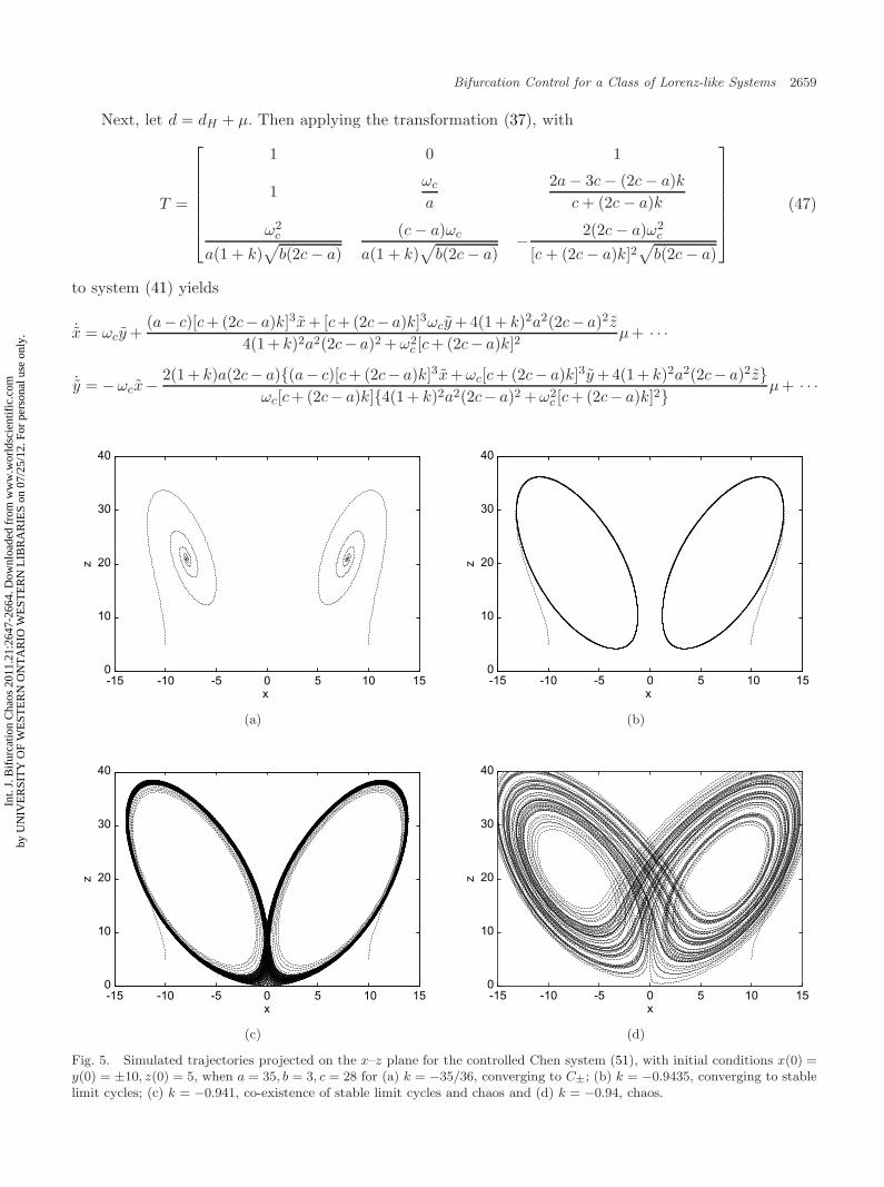
Fig. 5. Simulated trajectories projected on the x–z plane for the controlled Chen system (51), with initial conditions x(0) =y(0) = ±10, z(0) = 5, when a = 35, b = 3, c = 28 for (a) k = −35/36, converging to C±; (b) k = −0.9435, converging to stablelimit cycles; (c) k = −0.941, co-existence of stable limit cycles and chaos and (d) k = −0.94, chaos.

Int.

J. B

ifur

catio

n C

haos

201

1.21

:264

7-26

64. D

ownl

oade

d fr

om w

ww

.wor

ldsc

ient

ific

.com

by U

NIV

ER

SIT

Y O

F W

EST

ER

N O

NT

AR

IO W

EST

ER

N L

IBR

AR

IES

on 0

7/25

/12.

For

per

sona

l use

onl

y.

October 1, 2011 12:9 WSPC/S0218-1274 03000

2660 P. Yu & J. Lu

˙z = −2a(2c− a)(1+ k)c+ (2c− a)k

z − (a− c)[c+ (2c− a)k]3x+ [(2c− a)k]3ωcy + 4(1+ k)2a2(2c− a)2z4(1+ k)2a2(2c− a)2 + ω2

c [c+ (2c− a)k]2µ + · · ·

(48)

Now, applying the formula [Yu & Huseyin, 1988] to system (41) yields

v0 =−ω2

c [c + (2c − a)k]2

2{4(1 + k)2a2(2c − a)2 + ω2c [c + (2c − a)k]2} < 0,

and the Maple programs [Yu, 1998] gives v1 being a fourth-degree polynomial of k,

v1 =ω2

c [c + (2c − a)k](a − c)v1

8(2c − a){a2(2c − a)2(1 + k)2 + ω2c [c + (2c − a)k]2}[4a2(2c − a)2(1 + k)2 + ω2

c [c + (2c − a)k]2,

where v1 is given in (42). Therefore, the Hopf bifur-cation is supercritical (resp. subcritical) if v1 <0(v1 > 0); or equivalently if v1 < 0(v1 > 0) when(a − c)(2c − a) > 0.

To illustrate the application of the above ana-lytical results, let us choose the parameter valuesfor the Chen chaotic attractor: a = 35, c = 28. Forthis case, c < a < 2c, and

bH =7(26 + 27k)

4 + 3k, ωc = 7

√26 + 27k. (49)

In order to have ωc > 0, k must be chosen as

k > −2627

≈ −0.962962963, (50)

which guarantees bH > 0. For this case, v1 becomes

v1 = 7203(27k4 − 171k3 − 1032k2 − 1474k − 638),

which has four real roots:

k = −2.059664313, −1.142249478,

−0.9572404427, 10.49248757.

Combined with condition (50), we obtain that v1 <0 if

k ∈ (−0.9572404427, 10.49248757).

For b = 3, the equilibria C± of the uncon-trolled system are unstable. To stabilize C±, it isseen from (44) that k > −1 since 2c−a > 0, as wellas k < −(17/18). So the value of k for stabilizing C±is located in a very narrow interval (−1,−(17/18)).For example, we may choose k = −(35/36). Thesimulation result is shown in Fig. 5(a). It is notedthat this control is quite robust, i.e. the initial con-dition can be chosen far away from the equilibria.

If we choose k = −0.941, which yields bH =3.52676 > 3 and close to 3 (implying that the bifur-cation parameter µ is small). For this control value,C± are unstable, giving rise to bifurcation of stable

limit cycles, see Fig. 5(b). When k slightly increases,the system may exhibit co-existence of stable limitcycles and chaos, as shown in Fig. 5(c), or justchaotic motion [see Fig. 5(d)].

5. The Lu System

The Lu system is given by [Chen & Lu, 2003]

x = a(y − x), y = cy − xz, z = −bz + xy,

(51)

where a, b and c are real parameters, usually takingpositive values. The typical Lu’s chaotic attractoris shown in Fig. 1(c).

The Lu system (51) also has three equilibriumsolutions, C0, C+ and C−, given by

C0 : x0e = y0

e = z0e = 0,

C± : x±e = y±e = ±√

bc, z±e = c.(52)

Suppose a, b and c be positive. Then the character-istic polynomial associated with the equilibrium C0

is P0(λ) = (λ + 1)(λ + b)(λ− c), showing that C0 isunstable when c > 0. The characteristic polynomialassociated with the equilibria C± is given by

P±(λ) = λ3 + (a + b − c)λ2 + abλ + 2abc. (53)

It can be shown that when a + b − 3c > 0, C±are stable, and they lose stability at the criticalpoint:

bH = 3c − a, (54)

from which Hopf bifurcation occurs. When b >bH , C± are stable.


At the critical point defined in (54), the uncon-trolled Lu system (51) emerges to a Hopf

Int.

J. B

ifur

catio

n C

haos

201

1.21

:264

7-26

64. D

ownl

oade

d fr

om w

ww

.wor

ldsc

ient

ific

.com

by U

NIV

ER

SIT

Y O

F W

EST

ER

N O

NT

AR

IO W

EST

ER

N L

IBR

AR

IES

on 0

7/25

/12.

For

per

sona

l use

onl

y.

October 1, 2011 12:9 WSPC/S0218-1274 03000


bifurcation. At this critical point, the Jaco-bian of system (51) evaluated at C+ andC− has a real negative eigenvalue −2c and apurely imaginary pair ±i

√a(3c − a). With the

transformation,

x

y

z

=

±√

bc

±√bc

c

+ T

x

y

z

, (55)

where

T =

1 0 1

1ωc

a

a − 2ca

ω2c

a√

bc

(c − a)ωc√bc

2c(a − 3c)a√

bc

, (56)

we may transform (31) to

˙x = ωcy − a(a − c)x + aωcy + 4c2z

(a + c)(a − 4c)µ + · · ·

˙y = −ωcx +2c[a(a − c)x + aωcy + 4c2z]

ωc(a + c)(a − 4c)µ + · · ·

˙z = −2cz +a(a − c)x + aωcy + 4c2z

(a + c)(a − 4c)µ + · · ·

(57)

where µ = d − dH has been used.

Similarly, applying the formula and the Mapleprograms to system (51) yields the following focusvalues:

v0 =ω2

c

2(a + c)(a − 4c),

v1 =3ω2

c (a − c)(2a − 5c)8c(a + c)(4c − a)(c2 + ω2

c ).

It is easy to see that v1 < 0 if

c < a <52c.

For the parameter values of the typical Lu sys-tem: a = 30, b = 44/15, c = 111/5, we havebH = 183/5 > 44/15. Hence, the two equilibriaC± are unstable, and the trajectories are chaotic,as shown in Fig. 1(c). However, if we choose b closeto bH , then we may obtain stable limit cycles sincec < a < (5/2)c is satisfied for this case. For exam-ple, simulation results for b = 35 and b = 40 aredepicted in Figs. 6(a) and 6(b), respectively, con-firming the analytical predictions. These results aresimilar to the Chen system [see Fig. 4], not sensitiveto the initial conditions.


For the consistency, we use a similar control law asthat used for the Chen system, given by

u2 = kx(z − c), (58)

-50

-40

-30

-20

-10

0

10

20

30

40

50

-50 -40 -30 -20 -10 0 10 20 30 40 50

y

x

-50

-40

-30

-20

-10

0

10

20

30

40

50

-50 -40 -30 -20 -10 0 10 20 30 40 50

y

x

(a) (b)

Fig. 6. Simulated trajectories projected on the x–y plane for the uncontrolled Lu system (51) when a = 30, c = 111/5, withinitial conditions x(0) = 0, y(0) = ±2, z(0) = 15, for (a) b = 40, converging to C± and (b) b = 35, converging to stable limitcycles.

Int.

J. B

ifur

catio

n C

haos

201

1.21

:264

7-26

64. D

ownl

oade

d fr

om w

ww

.wor

ldsc

ient

ific

.com

by U

NIV

ER

SIT

Y O

F W

EST

ER

N O

NT

AR

IO W

EST

ER

N L

IBR

AR

IES

on 0

7/25

/12.

For

per

sona

l use

onl

y.

October 1, 2011 12:9 WSPC/S0218-1274 03000

2662 P. Yu & J. Lu

which, in turn, yields the closed-loop Lu system as

x = a(y − x),

y = cy − xz − kx(z − c), (59)

z = −bz + xy,

whose equilibria C0 and C± are not changed. Forthe controlled system (59), we have the followingresult for Hopf bifurcation control: Hopf bifurcationemerging from the equilibrium C± is supercritical ifthe feedback control gain coefficient k is chosen suchthat v1 < 0, where

v1 =(a − c)(a + ck)

8c[a2c2(1 + k)2 + ω2c (c + ck)2][4a2c2(1 + k)2 + ω2

c (c + ck)2]v1,

v1 = c4k4 + c3(a − 5c)k3 + c2a(a − 21c)k2 + ca(9a2 − 35ca + 2c2)k + 3a3(2a − 5c).

(60)

We give a detailed analysis below. First of all, a linear analysis shows that the equilibrium C0 isstable if (1 + k) < 0 and a − c > 0. Similarly, one can show that the two symmetric equilibria C± arestable if

1 + k > 0, a + ck > 0 and (a + b − c)(a + ck) > 2ac(1 + k). (61)

Hopf bifurcation for Lu system may occur at the critical point:

bH =c(a + c)(1 + k) − (a − c)2

a + ck. (62)

The eigenvalues evaluated at b = bH are

λ1,2 = ±i√

c(a + c)(1 + k) − (a − c)2, λ3 = −2ac(1 + k)a + ck

< 0, (63)

under the assumption: 1 + k > 0, a + ck > 0 and c(a + c)(1 + k) − (a − c)2 > 0.Let d = dH + µ. Then applying the transformation (37), with

T =

1 0 1

1ωc

a

a − 2c − ck

a + ck

ω2c

a(1 + k)√

bc

(c − a)ωc

a(1 + k)√

bc− 2cω2

c

(a + ck)2√

bc

(64)


˙x = ωcy +(a − c)(a + ck)3x + (a + ck)3ωcy + 4(1 + k)2a2c2z

4(1 + k)2a2c2 + ω2c (a + ck)2

µ + · · ·

˙y = −ωcx − 2ac(1 + k){(a − c)(a + ck)3x + (a + ck)3ωcy + 4a2c2(1 + k)2z}ωc(a + ck)[4(1 + k)2a2c2 + ω2

c (a + ck)2]µ + · · · (65)

˙z = −2ac(1 + k)a + ck

z − (a − c)(a + ck)3x + (a + ck)3ωcy + 4(1 + k)2a2c2z

4(1 + k)2a2c2 + ω2c (a + ck)2

µ + · · · .

The formula [Yu & Huseyin, 1988] and the Maple programs [Yu, 1998] that are employed to system (59)result in

v0 =−ω2

c (a + ck)2

2[4(1 + k)2a2c2 + ω2c (a + ck)2]

< 0,

and v1 being a fourth-degree polynomial of k, given in (60). Thus, when v1 < 0 (> 0) (or equivalently,v1 < 0 (> 0) if a > c), the Hopf bifurcation is supercritical (resp. subcritical).

To end this section, we present a couple of numerical simulation results to illustrate the application.For the typical parameter values of the Lu chaotic attractor: a = 30, c = 111/5, we have

bH =3(3050 + 3219k)

5(50 + 37k)and ωc =

35

√3050 + 3219k. (66)

Int.

J. B

ifur

catio

n C

haos

201

1.21

:264

7-26

64. D

ownl

oade

d fr

om w

ww

.wor

ldsc

ient

ific

.com

by U

NIV

ER

SIT

Y O

F W

EST

ER

N O

NT

AR

IO W

EST

ER

N L

IBR

AR

IES

on 0

7/25

/12.

For

per

sona

l use

onl

y.

October 1, 2011 12:9 WSPC/S0218-1274 03000


ωc > 0 requires

k > −30503219

≈ −0.9474992234, (67)

which guarantees bH > 0, and v1 then becomes

v1 =81625

(1874161k4 − 6838155k3 − 49763150k2

− 73097200k − 31875000),

which has fourth real roots:

k ≈ −2.002559540, −1.167523751,

−0.9378275909, 7.756559531.

Combined with the condition (67), we obtain thatv1 < 0 if

k ∈ (−0.9378275909, 7.756559531).

For b = 44/15, the equilibria C± of the uncon-trolled system are unstable. To stabilize C±, it isseen from (61) that −1 < k < −(25250/27343) ≈−0.9234539004. For example, we may choose k =−0.96. The simulation result is shown in Fig. 7(a).Again, it has been noted that under this control thebasins of the stable equilibria C± are quite large.

If we choose k = −0.923, this yields bH =2.985538 > 44/15 and close to 44/15. For thiscontrol value, C± are unstable, giving rise to

0

10

20

30

40

-15 -10 -5 0 5 10 15

z

x

0

10

20

30

40

0

10

20

30

40

-15 -10 -5 0 5 10 15

z

x

0

10

20

30

40

(a) (b)

0

10

20

30

40

-15 -10 -5 0 5 10 15

z

x

0

10

20

30

40

0

10

20

30

40

-15 -10 -5 0 5 10 15

z

x

(c) (d)

Fig. 7. Simulated trajectories projected on the x–z plane for the controlled Lu system (51) when a = 30, b = 44/15, c = 111/5for (a) k = −0.96, converging to C± with initial conditions x(0) = y(0) = ±1, z(0) = 15; (b) k = −0.923, convergingto stable limit cycles with initial conditions x(0) = ±8, y(0) = 0, z(0) = 5; (c) k = −0.92, co-existence of stable limitcycles and chaos with initial conditions x(0) = y(0) = ±8, z(0) = 15 and (d) k = −0.90, chaos with initial conditionsx(0) = y(0) = ±8, z(0) = 15.

Int.

J. B

ifur

catio

n C

haos

201

1.21

:264

7-26

64. D

ownl

oade

d fr

om w

ww

.wor

ldsc

ient

ific

.com

by U

NIV

ER

SIT

Y O

F W

EST

ER

N O

NT

AR

IO W

EST

ER

N L

IBR

AR

IES

on 0

7/25

/12.

For

per

sona

l use

onl

y.

October 1, 2011 12:9 WSPC/S0218-1274 03000

2664 P. Yu & J. Lu

bifurcation of stable limit cycles, as shown inFig. 7(b). When k is increased a little bit, the sys-tem can still have stable limit cycles but with chaosco-existing [see Fig. 7(c)] or just chaotic motion [seeFig. 7(c)].

6. Conclusion

In this paper, an early developed control formula isused for controlling Hopf bifurcations in a class ofLorenz-like systems. It has been shown that sim-ple control laws in a single quadratic term canbe applied, which not only leaves unchanged theequilibrium solutions of the original system, butcan also stabilize equilibrium solutions or peri-odic motions bifurcating from a Hopf critical point.This approach does not guarantee the global stabil-ity, but does not require ultimate boundedness oftrajectories, which is usually needed when apply-ing Lyapunov function method. In certain cases,it may be possible to suppress chaotic motions viaHopf bifurcation control, in particular, by stabiliz-ing equilibrium solutions. The method proposed inthis paper can be extended to consider other sin-gular cases, associated with double Hopf, Hopf-zeroand double zero.

Acknowledgments

This work was supported by the Natural Sci-ence and Engineering Research Council of Canada(NSERC) and National Natural Science Foundationof China (NNSFC).

References

Abed, E. H. & Fu, J.-H. [1987] “Local feedback stabiliza-tion and bifurcation control, I-II,” Syst. Cont. Lett. 8,467–473.

Berns, D., Moiola, J. L. & Chen, G. [2000] “Controllingoscillation amplitudes via feedback,” Int. J. Bifurca-tion and Chaos 10, 2815–2822.

Chen, D., Wang, H. O. & Chen, G. [2001] “Anti-controlof Hopf bifurcation,” IEEE Trans. Circuits Syst.-I 48,661–672.

Chen, G., Moiola, J. L. & Wang, H. O. [2000] “Bifur-cation control: Theories, methods, and applications,”Int. J. Bifurcation and Chaos 10, 511–548.

Chen, G. & Lu, J. [2003] Dynamics of the Lorenz Fam-ily: Analysis, Control and Synchronization (ChineseScience Press, Beijing).

Guckenheimer, J. & Holmes, P. [1993] Nonlinear Oscilla-tions, Dynamical Systems, and Bifurcations of VectorFields, 4th edition (Springer-Verlag, NY).

Hopf, E. [1942] “Abzweigung einer periodischen Losungvon stationaren Losung einers differential-systems,”Ber. Math. Phys. Kl. Sachs Acad. Wiss. Leipzig 94,1–22; Ber. Math. Phys. Kl. Sachs Acad. Wiss. LeipzigMath.-Nat. Kl. 95, 3–22.

Kang, W. & Krener, A. J. [2000] “Extended quadraticcontroller normal form and dynamic state feedbacklinearization of nonlinear systems,” SIAM J. Cont.Optim. 30, 1319–1337.

Laufenberg, M. J., Pai, M. A. & Padiyar, K. R. [1997]“Hopf bifurcation control in power systems with staticcompensation,” Int. J. Elect. Power Energy Syst. 19,339–347.

Lorenz, E. N. [1963] “Deterministic nonperiodic flow,”J. Atmos. Sci. 20, 130–141.

Lu, J. & Chen, G. [2002] “A new chaotic attractorcoined,” Int. J. Bifurcation and Chaos 12, 659–661.

Lu, J., Zhou, T., Chen, G. & Zhang, S. [2002a] “Localbifurcation of the Chen system,” Int. J. Bifurcationand Chaos 12, 2257–2270.

Lu, J., Zhou, T. & Zhang, S. [2002b] “Controlling Chenattractor using feedback function based on parame-ters identification,” Chin. Phys. 11, 12–16.

Lu, J. & Lu, J. [2003] “Controlling uncertain Lu systemusing linear feedback,” Chaos Solit. Fract. 17, 127–133.

Nayfeh, A. H., Harb, A. M. & Chin, C. M. [1996] “Bifur-cations in a power system model,” Int. J. Bifurcationand Chaos 6, 497–512.

Ono, E., Hosoe, S., Tuan, H. D. & Doi, S. [1998] “Bifur-cation in vehicle dynamics and robust front wheelsteering control,” IEEE Trans. Contr. Syst. Tech. 6,412–420.

Wang, H. O. & Abed, E. G. [1995] “Bifurcation controlof a chaotic system,” Automatica 31, 1213–1226.

Yu, P. & Huseyin, K. [1988] “A perturbation analysisof interactive static and dynamic bifurcations,” IEEETrans. Automat. Contr. 33, 28–41.

Yu, P. [1998] “Computation of normal forms via a per-turbation technique,” J. Sound Vibr. 211, 19–38.

Yu, P. [2000] “A method for computing center manifoldand normal forms,” Proc. Diff. Eqs. 1999 2, 832–837.

Yu, P. & G. Chen, G. [2004] “Hopf bifurcation controlusing nonlinear feedback with polynomial functions,”Int. J. Bifurcation and Chaos 14, 1683–1704.

Int.

J. B

ifur

catio

n C

haos

201

1.21

:264

7-26

64. D

ownl

oade

d fr

om w

ww

.wor

ldsc

ient

ific

.com

by U

NIV

ER

SIT

Y O

F W

EST

ER

N O

NT

AR

IO W

EST

ER

N L

IBR

AR

IES

on 0

7/25

/12.

For

per

sona

l use

onl

y.

bifurcation control for a class of lorenz …pyu/pub/preprints/yl_ijbc2011.pdf · october 1, 2011...

Documents