Bi

Ca

b

c

d

e

a

ARRA

KOHHTSCE

1

totea2meit

ttp

0

h0

Ecological Modelling 317 (2015) 93–106

Contents lists available at ScienceDirect

Ecological Modelling

journa l h om epa ge: www.elsev ier .com/ locate /eco lmodel

ifurcation analysis of an agent-based model for predator–preynteractions

. Colona,b,d,∗, D. Claessenb,c, M. Ghila,b,e

Laboratoire de Meteorologie Dynamique, Ecole Normale Supérieure, F-75231 Paris Cedex 05, FranceEnvironmental Research and Teaching Institute, Ecole Normale Supérieure, F-75231 Paris Cedex 05, FranceInstitut de Biologie de l’Ecole Normale Supérieure (CNRS UMR 8197, INSERM U1024), Ecole Normale Supérieure, 46 rue d’Ulm, 75005 Paris, FranceApplied Mathematics Department, Ecole Polytechnique, Route de Saclay, 91128 Palaiseau, FranceDepartment of Atmospheric and Oceanic Sciences, University of California at Los Angeles, Los Angeles, CA 90095-1565, USA

r t i c l e i n f o

rticle history:eceived 4 December 2014eceived in revised form 31 August 2015ccepted 2 September 2015

eywords:DEopf bifurcation

a b s t r a c t

The Rosenzweig–MacArthur model is a set of ordinary differential equations (ODEs) that provides anaggregate description of the dynamics of a predator–prey system. When including an Allee effect on theprey, this model exhibits bistability and contains a pitchfork bifurcation, a Hopf bifurcation and a hete-roclinic bifurcation. We develop an agent-based model (ABM) on a two-dimensional, square lattice thatencompasses the key assumptions of the aggregate model. Although the two modelling approaches – ODEand ABM – differ, both models exhibit similar bifurcation patterns. The ABM model’s behaviour is richerand it is analysed using advanced statistical methods. In particular, singular spectrum analysis is used to

eteroclinic bifurcationime series analysisingular spectrum analysisritical transitionarly-warning signals

robustly locate the transition between apparently random, small-amplitude fluctuations around a fixedpoint and stable, large-amplitude oscillations. Critical slowing down of model trajectories anticipates theheteroclinic bifurcation. Systematic comparison between the ABM and the ODE models’ behaviour helpsone understand the predator–prey system better; it provides guidance in model exploration and allowsone to draw more robust conclusions on the nature of predator–prey interactions.

© 2015 Elsevier B.V. All rights reserved.

. Introduction and motivation

Ecologists are more and more frequently asked to make predic-ions about the potential effects of specific changes to an ecosystemr a community of species. This demand is particularly vivid inhe context of climate change (Lavergne et al., 2010; Valladarest al., 2014) or resource management. It especially applies whennthropic harvesting is at play, as in fisheries (Lindegren et al.,010), or when biological factors might disturb an established com-unity of species, as in cases of non-endemic species invading an

cosystem (Crowl et al., 2008). Understanding these consequencess also relevant when the driver of changes is internal, in particularhrough evolutionary processes (Ferrière, 2009).

Whether the engine of change is external or internal, analysing

he consequences requires a comprehensive understanding ofhe community dynamics. Achieving such an understanding hasroven to be a challenging task. Observational and experimental

∗ Corresponding author at: CERES, Ecole Normale Supérieure, F-75231 Paris Cedex5, France. Tel.: +33 144323025

E-mail address: celian.colon@polytechnique.edu (C. Colon).

ttp://dx.doi.org/10.1016/j.ecolmodel.2015.09.004304-3800/© 2015 Elsevier B.V. All rights reserved.

data show that an ecological system composed of only two inter-acting species can exhibit non-trivial dynamics, such as bistabilityand oscillations (e.g., Fussmann et al., 2000). The importance ofnon-linear mechanisms in leading to such dynamics has motivatedtheoretical work on simple models to characterise the dynamicalregimes, identify and circumscribe basins of attraction, and locatebifurcations or regime shifts. To do so, ecologists have borrowedmathematical concepts and tools from other disciplines and tried avariety of modelling techniques, especially using systems of ordi-nary differential equations (ODEs).

A recent innovation is the development of agent-based models(ABMs), also called individual-based models in the ecological liter-ature. ABMs simulate systems described by the rules of interactionamong autonomous individuals. According to DeAngelis and Mooij(2005), some scholars view ABMs as exploratory tools that extendclassical aggregate models, whereas others suggest that ABMsprovide a methodological basis on which to build a novel researchparadigm (Grimm et al., 1999; Grimm and Railsback, 2005). In the

field of population dynamics, ABMs have helped investigate the roleof local interactions (Mccauley et al., 1993) and spatial dynamics(Dieckmann et al., 2000); they are also being increasingly employedto study evolutionary dynamics (Łomnicki, 1999; Gras et al., 2009).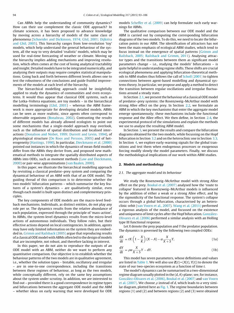

9 l Mode

Hcbpamtuttaattm

attmwcoossapepdeA2

bdgtttc

breIaemdot

Oqbi–bwafia–

4 C. Colon et al. / Ecologica

Can ABMs help the understanding of community dynamics?ow can their use complement the classic ODE approach? Inlimate sciences, it has been proposed to advance knowledgey moving across a hierarchy of models of the same class ofhenomena (Schneider and Dickinson, 1974; Ghil, 2001; Dijkstrand Ghil, 2005). This hierarchy ranges from low-resolution ‘toy’odels, which help understand the general behaviour of the sys-

em, all the way to very detailed ‘realistic’ models, which may besed for real-time forecasting of weather or climate. Moving uphe hierarchy implies adding mechanisms and improving resolu-ion, which often comes at the cost of losing analytical tractabilitynd insight. Detailed models have to be integrated numerically, andnalysing their outputs may require complex statistical manipula-ions. Going back and forth between different levels allows one toest the robustness of the conclusions and guide fruitful improve-

ents of the models at each level of the hierarchy.The hierarchical modelling approach could be insightfully

pplied to study the dynamics of communities and even ecosys-ems. It would thus appear that classical ODE systems, such ashe Lotka–Voltera equations, are toy models – in the hierarchical

odelling terminology (Ghil, 2001) – whereas the ABM frame-ork is more appropriate for developing detailed models. ABMs

an be seen as more realistic, since agents often correspond tobservable organisms (Bonabeau, 2002). Contrasting the resultsf different models has already allowed ecologists to point outome mechanisms that a single-model approach may overlook,uch as the influence of spatial distribution and localised inter-ctions (Donalson and Nisbet, 1999; Durrett and Levin, 1994), ofhysiological structure (De Roos and Persson, 2005) and of het-rogeneity (Hastings, 1990). In particular, Dieckmann et al. (2000)ointed out instances in which the dynamics of mean-field modelsiffer from the ABMs they derive from, and proposed new math-matical methods to integrate the spatially distributed aspects ofBMs into ODEs, such as moment methods (Law and Dieckmann,000) or pair-wise approximations (van Baalen, 2000).

In this paper, we illustrate the hierarchical modelling approachy revisiting a classical predator–prey system and comparing theynamical behaviour of an ABM with that of an ODE model. Theuiding thread of this comparison is to determine whether thewo models’ bifurcation patterns – which summarise the key fea-ures of a system’s dynamics – are qualitatively similar, evenhough each model is built upon distinct and complementary prin-iples.

The key components of ODE models are the macro-level feed-ack mechanisms. Individuals, as distinct entities, do not play anyole per se. The dynamics results from the relative abundance ofach population, expressed through the principle of ‘mass-action’.n ABMs, the system-level dynamics results from the micro-levelctions of autonomous individuals. They follow rules, but theirffective actions depend on local contingencies. In addition, agentsay have only limited information on the system they are embed-

ed in. Grimm and Railsback (2005) argue that reproducing resultsf a classical ODE model with ABMs often led to the design of modelshat are incomplete, not robust, and therefore lacking in interest.

In this paper, we do not aim to reproduce the outputs of anDE model with an ABM, neither do we want to perform anyuantitative comparison. Our objective is to establish whether theehaviour patterns of the two models are in qualitative agreement,

.e., whether the solution types – bistable, oscillatory and irregular are in one-to-one correspondence, including the transitionsetween these regimes of behaviour, as long as the two models,hile conceptually different, rely on the same key assumptions

bout the system under scrutiny. In addition, we are interested tond out – provided there is a good correspondence in regime typesnd bifurcations between the aggregate ODE model and the ABM

whether ideas on early warning that were developed for ODE

lling 317 (2015) 93–106

models Scheffer et al. (2009) can help formulate such early war-nings for ABMs.

The qualitative comparison between our ODE model and theABM is carried out by computing the corresponding bifurcationdiagrams of the two models. To do this, we need to locate the bifur-cation points in our ABM. The identification of attractors has notbeen the main emphasis of ecological ABM studies, which tend tofocus instead on the emergence of spatial patterns (Grimm andRailsback, 2005; Railsback and Grimm, 2011). Analysing attrac-tor types and the transitions between them as significant modelparameters change – i.e., studying the models’ bifurcations – isquite helpful in understanding regime shifts. These shifts are crucialecological phenomena and applying bifurcation-theoretical meth-ods to ABM studies thus follows the call of Scholl (2001) to tightenconnections between agent-based modelling and dynamical sys-tems theory. In particular, we propose and apply a method to detectthe transition between regular oscillations and irregular fluctua-tions around a steady state.

In Section 2.1, we present the behaviour of a classical ODE modelof predator–prey systems: the Rosenzweig–McArthur model withstrong Allee effect on the prey. In Section 2.2, we formulate anABM in which the key mechanisms that enter the aggregate modelemerge spontaneously; these mechanisms include the functionalresponse and the Allee effect. We then define, in Section 2.4, theexperimental protocol of the simulations and explain the methodswe use to analyse the resulting ABM model.

In Section 3, we present the results and compare the bifurcationdiagrams obtained for the two models, while focussing on the Hopfbifurcation in Section 3.2 and on the heteroclinic one in Section 3.3.In Section 4, we explore early-warning signals for the global tran-sitions and test them when endogenous processes or exogenousforcing modify slowly the model parameters. Finally, we discussthe methodological implications of our work within ABM studies.

2. Models and methodology

2.1. The aggregate model and its behaviour

We study the Rosenzweig–McArthur model with strong Alleeeffect on the prey. Boukal et al. (2007) analysed how the ‘route tocollapse’ featured in Rosenzweig–McArthur models is influencedby the addition of either a weak or a strong Allee effect, and bythe sigmoidicity of the functional response. The system’s collapseoccurs through a global bifurcation, characterised by an hetero-clinic orbit (van Voorn et al., 2007). Wang et al. (2011) performeda rigorous analysis of the model, and focussed on the existenceand uniqueness of limit cycles after the Hopf bifurcation. González-Olivares et al. (2006) performed a similar analysis with an Hollingtype III functional response.

Let X denote the prey population and Y the predator population.The dynamics is governed by the following two coupled ODEs:

dX

dt= rX

(1 − X

K

)(X − A) − ˛

X

X + SY, (1a)

dY

dt= �˛

X

X + SY − dY. (1b)

This model has seven parameters, whose definitions and valuesare listed in Table 1. We will also use Z(t) = (X(t), Y(t)) to denote thestate of our two-species ecosystem as a function of time t.

The model’s dynamics can be summarised in a two-dimensionalregime diagram usually plotted in the (d, A)-plane; see, for instance,

González-Olivares et al. (2006), Boukal et al. (2007) and van Voornet al. (2007). We choose � instead of d, which leads to a very simi-lar diagram, plotted here as Fig. 1. The regime boundaries betweenregions (1) and (2) and between regions (2) and (3) were obtained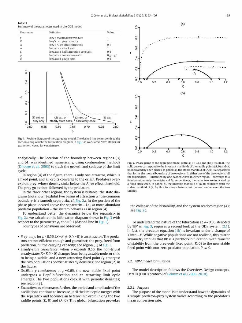

C. Colon et al. / Ecological Modelling 317 (2015) 93–106 95

Table 1Summary of the parameters used in the ODE model.

Parameter Definition Value

r Prey’s maximal growth rate 1K Prey’s carrying capacity 1A Prey’s Allee effect threshold 0.1˛ Predator’s attack rate 1S Predator’s half saturation constant 0.4� Predators’ conversion rate 0 ≤ � ≤ 1d Predator’s death rate 0.4

0.50 0.55 0.60 0.65 0.70 0.75 0.80

0.0

0.1

0.2

0.3

0.4

0.5

ρ

A

(1) ext. or prey only

(2) ext. or steady state co ex.

(3) ext. oroscillatory coex.

(4) ext.

Fig. 1. Regime diagram of the aggregate model. The dashed line corresponds to these

aa(c

aeT

gbpp

Fr

•

•

•

•

●

0.0 0.2 0.4 0.6 0.8 1.0 1.2

0.0

0.2

0.4

0.6

0.8

1.0

(a)

X

Y

●

●

PS

● ●

●

0.0 0.2 0.4 0.6 0.8 1.0 1.2

0.0

0.2

0.4

0.6

0.8

1.0

(b)

X

Y

● ● ●

Fig. 2. Phase plane of the aggregate model with (a) � = 0.61 and (b) � = 0.6808. Thesolid curves correspond to the invariant manifolds of the saddle points (A, 0) and (K,0), indicated by open circles. In panel (a), the stable manifold of (A, 0) is a separatrixthat forms the mutual boundary of two regions. In either one of the two regions, allthe trajectories – illustrated by one dashed curve in either region – converge to afixed point, namely the origin and PS, respectively; the latter two are indicated bya filled circle each. In panel (b), the unstable manifold of (K, 0) coincides with thestable manifold of (A, 0), thus forming a heteroclinic connection between the two

ection along which the bifurcation diagram in Fig. 3 is calculated. ‘Ext.’ stands forxtinction, ‘coex.’ for coexistence.

nalytically. The location of the boundary between regions (3)nd (4) was identified numerically, using continuation methodsDhooge et al., 2003) to track the growth and collapse of the limitycle.

In region (4) of the figure, there is only one attractor, which is fixed point, and all orbits converge to the origin. Predators over-xploit prey, whose density sinks below the Allee effect threshold.he prey go extinct, followed by the predators.

In the three other regions, the system is bistable: the state dia-rams (not shown) exhibit two basins of attraction whose commonoundary is a smooth separatrix, cf. Fig. 2a. In the portion of thehase plane located above the separatrix – i.e., at more abundantredator population – the system behaves as in region (4).

To understand better the dynamics below the separatrix inig. 2a, we calculated the bifurcation diagram shown in Fig. 3 withespect to the parameter �, at A = 0.1 (dashed line in Fig. 1).

Four types of behaviour are observed:

Prey-only: for � < 0.56, (X = K /= 0, Y = 0) is an attractor. The preda-tors are not efficient enough and go extinct; the prey, freed frompredation, fill the carrying capacity; see region (1) of Fig. 1.Steady-state coexistence: when � exceeds 0.56, the non-trivialsteady state (X = K, Y = 0) changes from being a stable node, or sink,to being a saddle, and a new attracting fixed point PS emerges:the two populations coexist at steady densities; see region (2) inthe figure.Oscillatory coexistence: at � = 0.65, the new, stable fixed pointundergoes a Hopf bifurcation and an attracting limit cycleemerges. The two populations coexist with periodic densities;see region (3).Extinction: as � increases further, the period and amplitude of the

oscillations continue to increase until the limit cycle merges withthe separatrix and becomes an heteroclinic orbit linking the twosaddle points (K, 0) and (A, 0). This global bifurcation provokes

saddles.

the collapse of the bistability, and the system reaches region (4);see Fig. 2b.

To understand the nature of the bifurcation at � = 0.56, denotedby ‘BP’ in Fig. 3, requires a second look at the ODE system (2.1).In fact, the predator equation (1b) is invariant under a change ofY into −Y. While negative populations are not realistic, this mirrorsymmetry implies that BP is a pitchfork bifurcation, with transferof stability from the prey-only fixed point (K, 0) to the new stablefixed point with non-zero predator population, Y /= 0.

2.2. ABM model formulation

The model description follows the Overview, Design concepts,Details (ODD) protocol of Grimm et al. (2006, 2010).

2.2.1. Purpose

The purpose of the model is to understand how the dynamics of

a simple predator–prey system varies according to the predator’smean conversion rate.

96 C. Colon et al. / Ecological Mode

0.4 0.5 0.6 0.7 0.8

0.0

0.2

0.4

0.6

0.8

1.0

(a) Prey

ρ

X

Ho

BP

He

0.4 0.5 0.6 0.7 0.8

0.0

0.2

0.4

0.6

0.8

1.0

(b) Predator

ρ

Y

Ho

BP

He

Fig. 3. Bifurcation diagram Z = Z(�) of the ODE model with respect to the parameter�, for A = 0.1; all the other parameters have the values in Table 1. (a) For the preypopulation X = X(�); and (b) for the predator population Y = Y(�). Solid lines rep-resent stable equilibria, dotted lines unstable equilibria. The prey-only fixed point(X = K, Y = 0) undergoes a one-sided pitchfork bifurcation, constrained by the posi-tivity of Y, and is denoted in the figure by BP, for branching point; see text for details.This bifurcation from a single to two fixed points is followed by a Hopf bifurcation(dh

2

cv

bbcoy

2

cdimTdr

2

b

Ho), with the dashed lines indicating the extrema of the limit cycles. The verticalashed line represents the location of the next, global bifurcation, via the birth of aeteroclinic orbit (He); see Fig. 2(b).

.2.2. Entities, state variables, and scalesAgents are of two types: predators and prey. Each agent is

haracterised by a specific identity number. The agent-level stateariables are their two spatial coordinates.

Agents evolve on a two-dimensional, square lattice L2, whoseoundary conditions are periodic, with no apriori limit on the num-er of agents that can be located in a cell; see Section 2.3 for thehoice of the lattice parameter values. One time step representsne week and simulations were run for 1000 weeks, i.e., about 19ears.

.2.3. Process overview and schedulingAt each time step, agents apply a set of rules, whose out-

omes depend on random variables and on the local environments,efined as the cell where the agent stands and the eight surround-

ng cells. One time step corresponds to the implementation of eightodules. First, prey follow the sequence move, reproduce and die.

hen predators act in the following order: move, hunt, reproduce,ie and migrate. Within each module, the order between agents isandom and updating is asynchronous.

.2.4. Design conceptsEmergence. The model was formulated so that the emergent

ehaviour of both population matches the key assumptions of the

lling 317 (2015) 93–106

Rosenzweig–MacArthur model with Allee effect on the prey, cf. Sec-tion 2.1; namely we expect the prey to exhibit logistic growth anda strong Allee effect, while the predator should collectively exhibita Holling type II functional response.

Sensing. Each agent can sense the presence of other agents intheir local environment.

Interactions. Three types of inter-agent interactions are explic-itly modelled. First, prey interact directly through mating: two preylocated in the same local environment can give birth to an offspring.Second, prey interact indirectly through density-dependence: mat-ing cannot occur if the number of prey in the local environmentexceeds a threshold. Third, predators and prey interact throughhunting: predators can hunt the prey located in their local envi-ronment.

Stochasticity. Many processes involve stochasticity. First, thereis spatial stochasticity: The movement of each agent is a two-dimensional random walk on L2. and each new offspring, prey andpredator alike, is assigned to a random location. Next, behaviouris stochastic: Most actions, including breeding, dying, hunting, areprobabilistic; specifically, they are realised if a random variable,generally drawn from a uniform distribution between 0 and 1,exceeds a threshold value.

Observation. The main data analysed are the prey and predatorpopulations as a function of time, X(t) and Y(t), respectively.

2.2.5. InitialisationThe model is initialised by setting the initial prey and predator

populations, X(0) and Y(0), and by assigning each agent a ran-dom location on the lattice L2. A wide range of initial populationsZ(0) = (X(0), Y(0)) was tested during preliminary model exploration.For the simulation experiments reported herein, we chose the ini-tial population pair (4000, 500), which leads to the most interestingdynamics.

2.2.6. Input dataThe model does not use input from external models or data files.

2.2.7. Submodels – prey modulesMove. Prey move to a randomly selected adjacent cell, whether

occupied or not.Reproduce. When a prey senses at least one other prey in its

local environment, and if the local density of prey does not exceeda saturation density S, it has a certain probability b to give birth toanother prey. This rule gives rise, at the population level, to twofeatures of the aggregate model: (i) At high density, reproductionis limited by S, which leads to a density-dependent growth rateand (ii) below a certain density, low mating probabilities lead toextinction. The latter phenomenon corresponds to the Allee effect,cf. Fig. 15 in Appendix A. Offspring are assigned to a random cell;doing so avoids prey immediately mating with their offspring.

Die. Each prey dies with probability v.

2.2.8. Submodels – predator modulesMove. Predators move to a randomly selected adjacent cell,

whether occupied or not.Hunt. When a predator senses prey in its local environment, it

has a certain chance s to catch and kill them, but it cannot, in anyevent, kill more than N prey at a time. This limited handling capacitygives rise, at the population level, to a functional response of typeII, cf. Fig. 17 in Appendix A.

Reproduce. After a successful hunt, a predator has a probability

� to breed a number of offspring equal to the number of prey itkilled. Like the prey, offspring are randomly located on the lattice.Predators who did not catch any prey cannot breed.

Die. Each predator dies with probability w.

C. Colon et al. / Ecological Modelling 317 (2015) 93–106 97

Table 2Summary of the parameters used in the ABM model.

Parameter Definition Value

L Number of cells along an edge of the squarelattice

100

b Prey’s probability to breed when meetinganother prey

1

S Prey’s local saturation density 5v Prey’s probability to die 0.05s Predator’s probability to succeed in hunting 0.1N Predator’s handling saturation 3

td

2

tTiw

tfpim

wemiow

mIaa0SS

2

csptTo.toss

bpgS

●

0 100 200 300 400 500 600

010

0020

0030

0040

0050

00

(a)κ = 0.41

t

X a

nd Y

●

0 100 200 300 400 500 600

010

0020

0030

0040

0050

00

(a)κ = 0.57

t

X a

nd Y

Fig. 4. Time series of the prey population X(�)(t) and the predator population Y(�)(t),shown as the upper and lower curves, respectively. Five simulations with � = 0.41and (b) five simulations with � = 0.57. In each panel, one of the simulations is shownas the heavy solid curve, the other four as light solid. The fluctuations in panel (a)are more irregular and have smaller amplitudes than those in panel (b). The use

� Predator’s mean conversion rate 0.21 ≤ � ≤ 0.7w Predator’s probability to die 0.1

Migrate. If all predators disappear but prey survive, a preda-or is added to the lattice; this model feature avoids prematureisappearance of predators due to purely stochastic phenomena.

.3. Choice of parameter values

The ABM has eight parameters, one more than the ODE model;hese eight parameters are defined, and their values given, inable 2. The objective choosing a set of parameters for the ABMs to approximate macro-level parameters of the aggregate model

ith corresponding ratios that emerge from the ABM simulations.We first focus on the Allee effect. In the ODE model, it is charac-

erised by its intensity, measured by the ratio A/K = 0.1. In the ABM,or L = 100, b = 1, S = 5, v = 0.05 and Z(0) = (4000, 500), the averagerey population in the absence of predators is denoted by K and

t equals 6080. This K is the emergent carrying capacity, whichirrors the explicitly-defined parameter K in the ODEs.By carrying out a series of simulations, we also observe that,

hen the prey population sinks below 520, it is more likely to goxtinct than to recover, cf. Fig. 15 in Appendix A. Additional experi-ents based on feedback control confirm that this value, denoted A,

s the emergent quantity that corresponds to the Allee effect thresh-ld A; see Appendix A for details. We obtain therewith A/K = 0.086,hich is close to A/K = 0.1 from Table 1.

The functional response, in turn, is characterised in the ODEodel by a logistic curve with a half-saturation constant S = 0.4.

n the ABM, for s = 0.1, M = 3 and w = 0.1, we observe that the aver-ge number of prey killed per predator plateaus at 0.3 when preyre abundant, i.e., X ≥ 9000. When X = 2750, the average kill rate is.15 = 0.30/2, which equals the emerging half-saturation constant

ˆ, cf. Fig. 17 in Appendix A. We obtain S/K = 0.45, which is close to/K = 0.4.

.4. Numerical experiments and analysis methods

We choose the predator’s mean conversion rate � as the bifur-ation parameter. For each value of � between 0.21 and 0.70, inteps of 0.01, we run the model 100 times and monitor the preyopulation X(t) and predator population Y(t). Each run differs byhe realisation of its random choices in agent actions and lasts forf = 1000 time steps, i.e., 1000 weeks �19 years. We obtain a setf 50 × 100 = 5000 time series X(�)

i(t) and Y (�)

i(t), with � = 0.21, 0.22,

. ., 0.70; i = 1, 2, . . ., 100; and t = 1, 2, . . ., 1000 . To characterisehe dynamics and identify threshold values, we carried out a seriesf statistical analyses on this output. To deal only with statisticallytationary data, we dropped the first 400 points of each time series,o our data set has 5000 × 600 = 3000 000 points.

First, for each value of �, we compute the probability distri-

utions of the corresponding run X(�) and Y(�), and derive theroportion of runs in which prey go extinct (extinction), predatorso extinct (prey-only), or both populations coexist (coexistence).econd, the time series in which the two species coexist were

of statistical and spectral methods helps locate the transition between these tworegime types.

analysed using spectral methods. A few examples of such timeseries are displayed in Fig. 4.

The ABM model was implemented using NetLogo (Wilenski,1999). The statistical analyses were performed with the R package(R Core Team, 2012).

It is clear from this figure that the behaviour differs widely as afunction of parameter value, with � = 0.41 in panel (a) and � = 0.57 inpanel (b). But, because of the stochastic processes that enter agentbehaviour, it is difficult to identify the structure of the underly-ing attractor: Are the irregular fluctuations of the simulated timeseries mere random noise around a fixed point, or do they exhibitoscillatory behaviour, which would point to a more complex attrac-tor? How can we locate the transition between the two seeminglydistinct regimes in Fig. 4a and b?

For each value of �, we analyse the time series in which the twospecies coexist using singular spectrum analysis (SSA) (Vautard andGhil, 1989; Vautard et al., 1992; Ghil et al., 2002) and Monte-CarloSSA (MC-SSA) (Allen and Smith, 1989; Ghil et al., 2002). These meth-ods have been widely used in climate dynamics and other areas,including population dynamics (Loeuille and Ghil, 1994). They arepresented succintly here and more thoroughly in Appendix B.

SSA decomposes a time series into elementary components that

can be classified into trends, oscillatory patterns and noise. Eachcomponent is associated with an eigenvector and an eigenvalueof the time series’s lag-covariance matrix. An oscillation, whether

9 l Modelling 317 (2015) 93–106

heibt

mgss1t

p5sab

2

ipwwiTr

vaaA1Tei

aiputattbptpoTop

3

3

cfita

0.2 0.3 0.4 0.5 0.6 0.7

0.0

0.2

0.4

0.6

0.8

1.0

κ

prop

ortio

n of

run

s

prey onlycoexistenceextinction

Fig. 5. Proportion of ABM runs reaching one of three possible regimes – prey-only(dashed line), coexistence (solid line) or extinction (dotted line) – as the parameter

8 C. Colon et al. / Ecologica

armonic or anharmonic, is captured by a pair of nearly equaligenvalues, whose associated eigenvectors have the same dom-nant frequency and are in phase quadrature. Typically, oscillatoryehaviour can be traced back to deterministic processes that con-ribute to generate the time series under study (Ghil et al., 2002).

MC-SSA tests the SSA results against a null hypothesis that isodelled by a simpler, purely stochastic process which could have

enerated it, typically white or red noise. Empirical analyses havehown that ecological time series, and in particular population timeeries, tend to have a ‘red-shifted’ spectrum (Pimm and Redfearn,988). Consequently, we have chosen to test the time series againsthe more stringent null hypothesis of red noise.

We are interested in detecting statistically significant oscillatoryatterns and apply MC-SSA to identify pairs of eigenvalues at the% confidence level or better, as explained in Appendix B. Pairs thaturvive this test will be called significant pairs of eigenvalues (SPEs)nd are indicative of oscillations produced by limit cycles, and noty purely stochastic effects.

.5. Choice of time horizon

Our objective is to identify our predator–prey system’s dynam-cal structure, namely the basins of attractions and bifurcationoints. In this perspective, how satisfactory is our choice of Tf = 1000eeks? To appraise the ecological significance of this time horizon,e evaluate the generation times of the two species, defined as the

nverse of the respective death rate. We denote these quantities byC for the predator and by TR for the prey. Since the predator deathate is w = 0.1 TC = 10 weeks.

The death rate of the prey is the sum of the natural death rate = 0.05 and a predation rate, while the latter is the product of theverage number of prey killed per predator and of the predatorbundance; this relationship is represented in Fig. 17 of Appendix. Since the predator population typically ranges between 0 and500, as seen in Section 3 below, TR varies between 8 and 20 weeks.he interval of 1000 weeks used in our study seems, therefore, longnough to capture ecologically significant dynamics, and it sufficesn order to avoid the transients due to a choice of initial state alone.

Is this time horizon of 1000 weeks also sufficient in order toccount for long-term behaviour? Due to the model’s stochasticngredients, and given long enough simulation intervals, it is quiteossible that particular sequences of events that are a priori verynlikely will occur and lead trajectories to change basins of attrac-ion. Since there is no external input of prey, extinction is the onlybsolutely inescapable regime, into which all trajectories will even-ually fall. Focusing on genuinely asymptotic behaviour only wouldherefore prevent us from identifying the basins of attraction andifurcation points that, according to the ODE model, do seem tolay an important role. The ecologically significant dynamics mighthus lie in what can be considered, from an asymptotic stand-oint, as merely very long transients (Hastings, 2004). We carriedut additional experiments with Tf = 10 000 weeks ≈200 years andf = 100 000 weeks ≈2000 years to assess the robust persistencef each attractor basin identified, along with evaluating associatedrobabilities.

. ABM model results

.1. Dominant regime and fixed points

As in the ODE model, if the initial predator population is large

ompared to the initial prey population, the prey will go extinctrst, followed by the predators. For smaller initial predator popula-ions, several regimes can occur: extinction, prey-only or coexistence,s shown in Fig. 5. As the parameter � – which measures the

� varies, 0.21 ≤ � ≤ 0.70.

reproduction efficiency of the predator – increases, two transi-tions are detected: the first one between 0.35 and 0.36, where thedominant regime switches from prey-only to coexistence, and thesecond one between 0.60 and 0.61, where it changes from coexis-tence to extinction.

During this second transition, we observe a small peak in thenumber of occurrences of the prey-only regime. In these simula-tions, the combination of stochastic events with moderate � valuesleads to the following scenario: the predators deplete the prey pop-ulation down to a level close to A, which is insufficient for predatorsurvival, while the prey population – being freed from predationand with the help of positive stochastic events – is able to persist.For higher � values, predators deplete the prey population morerapidly, so that it falls well below A and thus induces extinction ofboth populations.

In Fig. 6 we plot, for each �-value, the distribution of the popu-lations {X(�)

i(t)} and {Y (�)

i(t)} over the realisations i = 1, . . ., 100,

and over the 600-week–long time interval 401 ≤ t ≤ 1000. Dur-

ing the first transition, at � � 0.36, the average populations Z(�) =

(X(�), Y (�)) change rather smoothly, whereas the second transition,at � � 0.61, is marked by a sudden drop in both population aver-ages. Before the collapse, the range of their values increases ratherstrikingly.

In the prey-only steady state, the prey population fluctuatesaround K = 6080, i.e., around a value that is almost 12 times theAllee effect threshold. At this level, only a series of extremely highdeath rates – combined with very unlikely spatial distributions thatseverely limit reproduction – could lead the prey towards extinc-tion. The probability of having more than 500 prey dying at once,i.e., still a fairly small number that only corresponds to one-eleventhof the road to extinction is less than 10−30. This basin of attraction isso deep that, even on geological time scales, the prey-only regimecan be considered as stable.

The coexistence regime requires a more thorough examination.The presence of predators creates new opportunities for adversestochastic events; still, their probabilities remain extremely low formoderate �-values. For � = 0.57, additional, 2000-year-long simu-lations still show that less than 2% of the runs lead to extinction.As we approach the transition at � � 0.61, the depth of the basin ofattraction decreases and coexistence is less and less likely to per-sist. Had we initially set the duration of the simulations to 2000years, rather than 200 years, as in Fig. 6, the transition value of �

would be 0.59 instead of 0.61. This difference is still quite moderatewith respect to the size of the basins of attraction, in terms of theparameter �, as shown in Fig. 5. The robustness of our results upon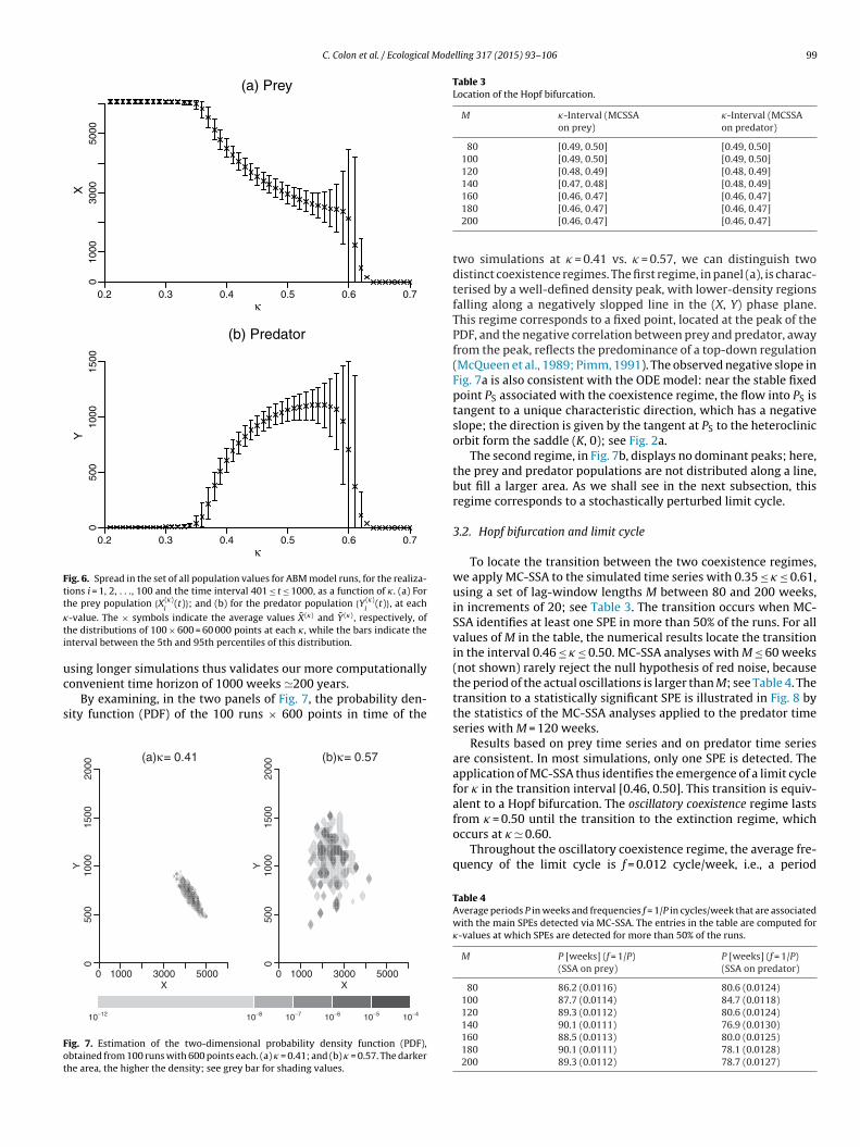

C. Colon et al. / Ecological Modelling 317 (2015) 93–106 99

0.2 0.3 0.4 0.5 0.6 0.7

010

0030

0050

00

κ

X(a) Pr ey

0.2 0.3 0.4 0.5 0.6 0.7

050

010

0015

00

κ

Y

(b) Predator

Fig. 6. Spread in the set of all population values for ABM model runs, for the realiza-tions i = 1, 2, . . ., 100 and the time interval 401 ≤ t ≤ 1000, as a function of �. (a) Forthe prey population {X(�)(t)}; and (b) for the predator population {Y (�)(t)}, at each

�ti

uc

s

Fot

Table 3Location of the Hopf bifurcation.

M �-Interval (MCSSAon prey)

�-Interval (MCSSAon predator)

80 [0.49, 0.50] [0.49, 0.50]100 [0.49, 0.50] [0.49, 0.50]120 [0.48, 0.49] [0.48, 0.49]140 [0.47, 0.48] [0.48, 0.49]

i i

-value. The × symbols indicate the average values X(�) and Y (�) , respectively, ofhe distributions of 100 × 600 = 60 000 points at each �, while the bars indicate thenterval between the 5th and 95th percentiles of this distribution.

sing longer simulations thus validates our more computationally

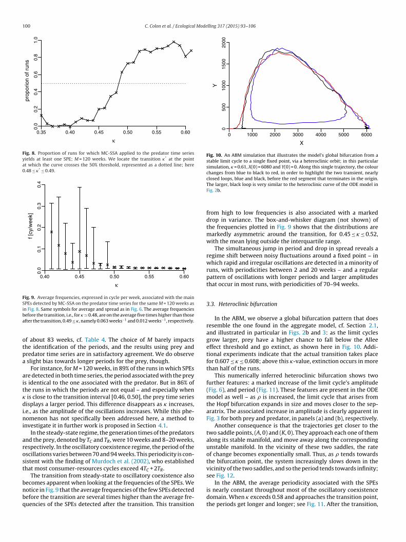
onvenient time horizon of 1000 weeks �200 years.

By examining, in the two panels of Fig. 7, the probability den-ity function (PDF) of the 100 runs × 600 points in time of the

0 1000 3000 5000

050

010

0015

0020

00

X

Y

(a)κ = 0.41

0 1000 3000 5000

050

010

0015

0020

00

X

Y

(b)κ = 0.57

10−12 10 −8 10−7 10−6 10−5 10−4

ig. 7. Estimation of the two-dimensional probability density function (PDF),btained from 100 runs with 600 points each. (a) � = 0.41; and (b) � = 0.57. The darkerhe area, the higher the density; see grey bar for shading values.

160 [0.46, 0.47] [0.46, 0.47]180 [0.46, 0.47] [0.46, 0.47]200 [0.46, 0.47] [0.46, 0.47]

two simulations at � = 0.41 vs. � = 0.57, we can distinguish twodistinct coexistence regimes. The first regime, in panel (a), is charac-terised by a well-defined density peak, with lower-density regionsfalling along a negatively slopped line in the (X, Y) phase plane.This regime corresponds to a fixed point, located at the peak of thePDF, and the negative correlation between prey and predator, awayfrom the peak, reflects the predominance of a top-down regulation(McQueen et al., 1989; Pimm, 1991). The observed negative slope inFig. 7a is also consistent with the ODE model: near the stable fixedpoint PS associated with the coexistence regime, the flow into PS istangent to a unique characteristic direction, which has a negativeslope; the direction is given by the tangent at PS to the heteroclinicorbit form the saddle (K, 0); see Fig. 2a.

The second regime, in Fig. 7b, displays no dominant peaks; here,the prey and predator populations are not distributed along a line,but fill a larger area. As we shall see in the next subsection, thisregime corresponds to a stochastically perturbed limit cycle.

3.2. Hopf bifurcation and limit cycle

To locate the transition between the two coexistence regimes,we apply MC-SSA to the simulated time series with 0.35 ≤ � ≤ 0.61,using a set of lag-window lengths M between 80 and 200 weeks,in increments of 20; see Table 3. The transition occurs when MC-SSA identifies at least one SPE in more than 50% of the runs. For allvalues of M in the table, the numerical results locate the transitionin the interval 0.46 ≤ � ≤ 0.50. MC-SSA analyses with M ≤ 60 weeks(not shown) rarely reject the null hypothesis of red noise, becausethe period of the actual oscillations is larger than M; see Table 4. Thetransition to a statistically significant SPE is illustrated in Fig. 8 bythe statistics of the MC-SSA analyses applied to the predator timeseries with M = 120 weeks.

Results based on prey time series and on predator time seriesare consistent. In most simulations, only one SPE is detected. Theapplication of MC-SSA thus identifies the emergence of a limit cyclefor � in the transition interval [0.46, 0.50]. This transition is equiv-alent to a Hopf bifurcation. The oscillatory coexistence regime lasts

from � = 0.50 until the transition to the extinction regime, whichoccurs at � � 0.60.

Throughout the oscillatory coexistence regime, the average fre-quency of the limit cycle is f = 0.012 cycle/week, i.e., a period

Table 4Average periods P in weeks and frequencies f = 1/P in cycles/week that are associatedwith the main SPEs detected via MC-SSA. The entries in the table are computed for�-values at which SPEs are detected for more than 50% of the runs.

M P [weeks] (f = 1/P)(SSA on prey)

P [weeks] (f = 1/P)(SSA on predator)

80 86.2 (0.0116) 80.6 (0.0124)100 87.7 (0.0114) 84.7 (0.0118)120 89.3 (0.0112) 80.6 (0.0124)140 90.1 (0.0111) 76.9 (0.0130)160 88.5 (0.0113) 80.0 (0.0125)180 90.1 (0.0111) 78.1 (0.0128)200 89.3 (0.0112) 78.7 (0.0127)

100 C. Colon et al. / Ecological Modelling 317 (2015) 93–106

0.35 0.40 0.45 0.50 0.55 0.60

0.0

0.2

0.4

0.6

0.8

1.0

κ

prop

orio

n of

run

s

Fig. 8. Proportion of runs for which MC-SSA applied to the predator time seriesyields at least one SPE; M = 120 weeks. We locate the transition �* at the pointat which the curve crosses the 50% threshold, represented as a dotted line; here0.48 ≤ �* ≤ 0.49.

0.40 0.45 0.50 0.55 0.60

0.0

0.1

0.2

0.3

0.4

κ

f [cy

/wee

k]

Fig. 9. Average frequencies, expressed in cycle per week, associated with the mainSPEs detected by MC-SSA on the predator time series for the same M = 120 weeks asin Fig. 8. Same symbols for average and spread as in Fig. 6. The average frequenciesba

otpa

ait�dini

arost

bnbq

●

0 1000 2000 3000 4000 5000 6000

050

010

0015

0020

00

X

Y

Fig. 10. An ABM simulation that illustrates the model’s global bifurcation from astable limit cycle to a single fixed point, via a heteroclinic orbit; in this particularsimulation, � = 0.61, X(0) = 6080 and Y(0) = 0. Along this single trajectory, the colourchanges from blue to black to red, in order to highlight the two transient, nearlyclosed loops, blue and black, before the red segment that terminates in the origin.

efore the transition, i.e., for � � 0.48, are on the average five times higher than thosefter the transition, 0.49 ≤ �, namely 0.063 weeks−1 and 0.012 weeks−1, respectively.

f about 83 weeks, cf. Table 4. The choice of M barely impactshe identification of the periods, and the results using prey andredator time series are in satisfactory agreement. We do observe

slight bias towards longer periods for the prey, though.For instance, for M = 120 weeks, in 89% of the runs in which SPEs

re detected in both time series, the period associated with the preys identical to the one associated with the predator. But in 86% ofhe runs in which the periods are not equal – and especially when

is close to the transition interval [0.46, 0.50], the prey time seriesisplays a larger period. This difference disappears as � increases,

.e., as the amplitude of the oscillations increases. While this phe-omenon has not specifically been addressed here, a method to

nvestigate it in further work is proposed in Section 4.1.In the steady-state regime, the generation times of the predators

nd the prey, denoted by TC and TR, were 10 weeks and 8–20 weeks,espectively. In the oscillatory coexistence regime, the period of thescillations varies between 70 and 94 weeks. This periodicity is con-istent with the finding of Murdoch et al. (2002), who establishedhat most consumer-resources cycles exceed 4TC + 2TR.

The transition from steady-state to oscillatory coexistence alsoecomes apparent when looking at the frequencies of the SPEs. We

otice in Fig. 9 that the average frequencies of the few SPEs detectedefore the transition are several times higher than the average fre-uencies of the SPEs detected after the transition. This transition

The larger, black loop is very similar to the heteroclinic curve of the ODE model inFig. 2b.

from high to low frequencies is also associated with a markeddrop in variance. The box-and-whisker diagram (not shown) ofthe frequencies plotted in Fig. 9 shows that the distributions aremarkedly asymmetric around the transition, for 0.45 ≤ � ≤ 0.52,with the mean lying outside the interquartile range.

The simultaneous jump in period and drop in spread reveals aregime shift between noisy fluctuations around a fixed point – inwhich rapid and irregular oscillations are detected in a minority ofruns, with periodicities between 2 and 20 weeks – and a regularpattern of oscillations with longer periods and larger amplitudesthat occur in most runs, with periodicities of 70–94 weeks.

3.3. Heteroclinic bifurcation

In the ABM, we observe a global bifurcation pattern that doesresemble the one found in the aggregate model, cf. Section 2.1,and illustrated in particular in Figs. 2b and 3: as the limit cyclesgrow larger, prey have a higher chance to fall below the Alleeeffect threshold and go extinct, as shown here in Fig. 10. Addi-tional experiments indicate that the actual transition takes placefor 0.607 ≤ � ≤ 0.608; above this �-value, extinction occurs in morethan half of the runs.

This numerically inferred heteroclinic bifurcation shows twofurther features: a marked increase of the limit cycle’s amplitude(Fig. 6), and period (Fig. 11). These features are present in the ODEmodel as well – as � is increased, the limit cycle that arises fromthe Hopf bifurcation expands in size and moves closer to the sep-aratrix. The associated increase in amplitude is clearly apparent inFig. 3 for both prey and predator, in panels (a) and (b), respectively.

Another consequence is that the trajectories get closer to thetwo saddle points, (A, 0) and (K, 0). They approach each one of themalong its stable manifold, and move away along the correspondingunstable manifold. In the vicinity of these two saddles, the rateof change becomes exponentially small. Thus, as � tends towardsthe bifurcation point, the system increasingly slows down in thevicinity of the two saddles, and so the period tends towards infinity;see Fig. 12.

In the ABM, the average periodicity associated with the SPEs

is nearly constant throughout most of the oscillatory coexistencedomain. When � exceeds 0.58 and approaches the transition point,the periods get longer and longer; see Fig. 11. After the transition,

C. Colon et al. / Ecological Modelling 317 (2015) 93–106 101

0.56 0.57 0.58 0.59 0.60 0.61 0.620.00

40.

008

0.01

20.

016

κ

f [cy

/wee

k]

Fig. 11. Box-and-whisker diagram of the frequencies, expressed in cycles per week,associated with the main SPEs detected by MC-SSA on the predator time series forM = 120 weeks. The bottom and top of the boxes are the first and third quartiles,the heavy horizontal lines inside the boxes are the medians, and the ends of thewhiskers are the extrema. The width of a box is proportional to the square root ofthe number of observations. There is a marked decrease in the frequencies of theSPEs for � ≥ 0.58. The results for the prey time series exhibit a similar pattern (nots

io

tpsMwtu

OttTwep

td

F

0.56 0.57 0.58 0.59 0.60 0.61 0.62

050

010

0020

0030

00

κ

aver

age

min

imum

val

ue o

f X

●●

●

●

●●●

●●

●

hown).

n the few runs where extinction does not occur, the periods keepn increasing, but at a slower pace.

The occurrence of a slowing down in the ABM is consistent withhe ODE model. As predators become more efficient, they push therey towards the Allee effect threshold; see Fig. 13. The fewer preyurvive, the slower they find partners and repopulate the lattice.ore acute depletions of prey lead to larger depletions of predators,hose recovery is delayed. This delay allows prey to get closer to

he carrying capacity, before predators recover. This cycle repeatsntil prey fail to recover and go extinct.

The period in the ABM, though, increases less than that in theDE model. Because of the discreteness of the state variables and

he resulting demographic stochasticity, trajectories do not stay onhe limit cycle along which the asymptotic slowing down occurs.hey either move back into the hinterland of the coexistence region,here the dynamics is faster, or cross the boundary and fall into

xtinction. Hence, due to the noise in the ABM, the increase ineriodicity remains moderate.

The implications of this slowing-down phenomenon for a poten-ial early warning ahead of the heteroclinic bifurcation will be

iscussed in Section 4.2.

0.650 0.655 0.660 0.665 0.670 0.675 0.680 0.685

1020

5010

020

050

0

ρ

Per

iod

[wee

ks]

ig. 12. Period of the limit cycle of the ODE model, in log scale, as a function of �.

Fig. 13. Box-and-whisker diagram of the average minimum prey abundance duringoscillations, as a function of �. Same conventions as in Fig. 11. The horizontal dashedline shows the Allee effect threshold A.

4. Concluding remarks

4.1. Summary and discussion

Even simple ecological systems can exhibit complex dynamics.In this paper, we have shown that an approach based on a hierar-chy of models can be highly effective in exploring such a complexsystem. At one end of the modelling spectrum, ABMs are arguablybest adapted for ‘realistic’ modelling, inasmuch as many observedfeatures of the individuals that are an ecosystem’s building blockscan be plugged in directly. We argue that ABMs should, as muchas possible, be developed in conjunction with simpler ‘toy’ models.Doing so facilitates the analysis, allows one to compare results, andfinally to draw robust conclusions. This back-and-forth betweendifferent models is also well illustrated by Siekmann (2015) in thecase of the dynamics of a two-strain infection process.

In this paper, we focused on a simple predator–prey system,using a deterministic ODE model and a stochastic ABM. RunningABM simulations and analysing their output were computationallyintensive and time-consuming tasks. For instance, the applicationof MC-SSA required the generation and analysis of 200 surrogatedata – 100 for the prey time series, and 100 for the predator timeseries – for each one of the 100 simulations run per � value. Giventhe 50 � values used, this yields 200 × 100 × 50 = 106 runs.

Nevertheless, the analysis could be conducted efficientlybecause it was guided by the existence of a much simpler and,in part, analytically tractable ODE model. The process was quitestraightforward in this case, since the ABM model was built a priorito share certain features of the aggregate model. Still, the strikingsuccess of the guidance provided by the simpler model suggeststhat this approach might be of great interest across a richer hierar-chy of models.

An interesting addition would be a model of intermediate com-plexity based on stochastic differential equations (SDEs), whichcombine some of the stochastic features of ABMs with the simpledeterministic ones of ODE models. Bifurcations of nonlinear SDEshave been studied by Kuehn (2011), and their usefulness in theclimate modelling hierarchy has been demonstrated by Ghil et al.(2008) and Chekroun and Ghil (2011), among others. In particular,SDEs could be used to explore the possible stochastic origin of thebias towards larger periodicities of the prey time series observedin Tab. 4. An explanation might be that stochastic perturbations

occasionally block the oscillations of the prey population, leadingto larger average periods. To investigate this hypothesis, one couldperturb the deterministic aggregate model by adding multiplicativenoise – first to one ODE at a time, then to both.

1 l Mode

waumtotdssta

aismlttat

tLagchi

omoso‘dsacmn2

tOsFtnsc

ataub

4

r‘

02 C. Colon et al. / Ecologica

The guidance provided by the ODE model helped us decide onhich parameter to control and which bifurcations to expect. But to

ctually perform the analysis, we needed to carefully design sim-lation experiments and develop or adapt appropriate statisticalethodology. Simple tests were used to detect transitions between

he main regimes. For more challenging tasks, such as the detectionf the Hopf bifurcation, we tapped into well-established methods ofime series analysis. The advanced spectral methods of SSA and itserivatives were used to distinguish large-amplitude, regular andtable oscillations from small-amplitude, irregular fluctuations. Atatistical test based on a Monte Carlo algorithm was used to iden-ify oscillatory patterns that significantly differ, at the 5% level, from

red noise process.Whether applied to the predator or to the prey time series, the

nalysis indicates a similar location of the Hopf bifurcation, whichn addition was robust to changes of the window-width. The tran-ition region from steady states to oscillatory behaviour was alsoarked by a sharp decrease in the mean and variance of the oscil-

ations’ frequencies; this decrease provides further evidence for aransition from a regime of small, rapid and erratic fluctuationso a regime of ample, regular and stable oscillations. MC-SSA thusppears to be well-suited for the detection and analysis of oscilla-ory dynamics in ABM-simulated time series.

Further methods of time series analysis could be integrated intohe toolbox of ABM users. For instance, Kolmogorov entropy oryapunov exponents could provide further insights into whether

deterministically chaotic process has participated in generating aiven time series (Kantz, 1994; Schouten et al., 1994). The appli-ation of such observables to experimental time series is oftenampered by the limited length and accuracy of such series; this

mpediment does not exist for ABM-generated output.Time series analysis alone does, however, not take advantage

f the modeller’s ability to freely design simulation experi-ents. The application of control-based methods – such as the

ne used to locate the Allee effect threshold, cf. Appendix A –eems to be a promising approach for the dynamical analysisf ABMs. Besides, Kevrekidis and colleagues have developed an

equation-free’ approach, in which macroscopic variables and theirerivatives are obtained from microscopically defined models –uch as ABMs – through the systematic implementation of a set ofppropriately initialised simulations (Kevrekidis et al., 2004). Thisoarse-graining process enables one to use numerical bifurcationethods and it was applied to ABMs describing an epidemiological

etwork (Reppas et al., 2010) and a financial market (Siettos et al.,012).

Our approach to bifurcation in ABMs conceptually differs fromhe classic mathematical framework for bifurcation analysis inDEs. In the latter, bifurcations are precisely defined using the

ame type of mathematical objects as those used to build the model.or instance, Hopf bifurcations can be precisely detected throughhe application of the Poincaré–Andronov–Hopf theorem. Wheneeded, numerical methods are employed to compute the localtructure of the Jacobian matrix and identify a bifurcation. Bifur-ations are, in other words, endogenous to the model.

In this paper we used MC-SSA and defined the Hopf bifurcations the point at which, in a majority of simulations, we observedhe emergence of oscillations that are different from a red noise, at

preset significance level. In this approach, the analytical methodsed is as important as the ABM formulation for the analysis of theifurcations.

.2. Early warnings of a global bifurcation

Studying a hierarchy of models is also instructive in testingesults on critical transitions and their ex-ante detection throughearly-warning signals’. The heteroclinic bifurcation present in both

lling 317 (2015) 93–106

of our models belongs to the class of global bifurcations, which arestructurally unstable and hence harder to detect numerically (Haleand Koc ak, 1991). Moreover, Scheffer et al. (2009) and Boettigeret al. (2013) noted, in fact, that the early-warning signals of suchbifurcations have been studied relatively little: most early-warningsignals proposed in the literature – namely slowing down of trajec-tories, as well as increased variance, autocorrelation and skewness– derive from the properties of the saddle-node bifurcation, whichbelongs to the class of local bifurcations (Hale and Koc ak, 1991).

In Section 3.3 we have seen that, in both models, some keyfeatures of the limit cycles change as the system approaches theheteroclinc bifurcation. The limit cycles get closer to the boundaryof the basin of attraction, their amplitudes increase, and the oscil-lations slow down as a result of approaching the infinite period ofthe exact heteroclinic orbit.

This type of period increase differs from the phenomenonknown as critical slowing down (CSR) (Wissel, 1984; Nes andScheffer, 2007). The latter refers to the increase of return time afterperturbations near a threshold, due to the real part of the dominanteigenvalue of a fixed point approaching zero. CSR has been theo-retically demonstrated, and empirically tested, for a range of localbifurcations, especially for saddle-node bifurcations (Boettigeret al., 2013), and it is interpreted as a loss of resilience in the vicinityof a tipping point (Nes and Scheffer, 2007; Dai et al., 2012).

In the ODE model, after the Hopf bifurcation, the unstable fixedpoint of region (4) of Fig. 1 becomes more repellent as � increases,and the geometry of the flow near it changes. As a consequence,trajectories become gradually more affected by the specific dynam-ics that occurs in the vicinity of the two saddle points, (A, 0) and(K, 0). The slowing down does not originate from the real partof any eigenvalue vanishing; instead, it is due to a geometricalchange of the basin of attraction. Another difference with respectto CSR is that this phenomenon is not observed through exogenousperturbations, but affects the endogenous dynamics of the sys-tem, i.e., the limit cycle. Even so, a broad-brush interpretation thatis similar to CSR could be proposed, namely, as the parameter� – which is the conversion rate of the predator – increases,each population, which is periodically perturbed by the other one,recovers more and more slowly, i.e., it is less resilient.

The system as a whole is also less resilient, as it lies closer tothe boundary of the basin of attraction, i.e., it is more ‘precarious’,in the sense of Walker et al. (2004). This aspect is more adequatelycaptured by the amplitude of the limit cycles, to be compared withsome known boundaries of the basin, such as the Allee effect thresh-old.

The slowing down near the two saddle points is also expectedto induce an asymmetry in the distribution of the populationabundance. This asymmetry can be captured by computing theskewness of the probability distribution in the time series. Guttaland Jayaprakash (2008) have proposed skewness � as a potentialearly-warning signal for local bifurcation: � is simply a distribu-tion’s third standardised moment, and it measures its degree ofasymmetry. Given a random variable Z, with mean � and standarddeviation �, skewness � is defined as

� = E[(

Z − �

�

)]. (2)

Results presented in Fig. 14 show that, in the ODE model, theasymmetry of both trajectories markedly increases as � approachesthe bifurcation value 0.6801. The system slows down in regionswith few predators, and accelerates when predators are abundant,so that the oscillations of the predator population are unbalanced

towards low values. We can show analytically that, due to thestrong Allee effect, prey recovery near (A, 0) is much quicker thanpredator recovery near (K, 0). As a consequence, the slowing downnear (K, 0) is more marked than the slowing down near (A, 0), and

C. Colon et al. / Ecological Mode

Ffb

tWpbfd

ssbtrmm(sho

pssfaowt

4

actiw

ig. 14. Skewness � of the predator and prey time series (a) in the ODE model as aunction of � and (b) in the ABM model as a function of �. In panel (b), the verticalar represents the interquartile range.

he prey distribution tends to be unbalanced towards high values.hile Guttal and Jayaprakash (2008) applied skewness to study

erturbed trajectories around a fixed point in the vicinity of a localifurcation, we see in Fig. 14a that this measure can also be usedor oscillatory regimes approaching a global bifurcation, but forifferent dynamical reasons.

Skewness results for the ABM differ widely from the ODE ones;ee Fig. 14b. Before the transition, which occurs for � � 0.60, thekewness of predator time series moderately increases in average,ut we do not observe a decrease for the prey time series. Moreover,he signs of the skewness seem surprising with regards to the ODEesults. This points out at one major difference between the twoodels. In the ABM, the mating requirements for prey, which is notodelled in the ODE, significantly slows down the systems in the

A, 0) region. In the ODE, the situation is opposite: because of thetrong Allee effect, the growth rate of the prey in the (A, 0) region isigher than in the other regions. The two models therefore exhibitspposite results.

The preceding discussion stresses an interesting slowing downhenomenon, which is different from CSR but, like it, also has con-iderable potential as an early warning signal. Skewness, however,eems to be more ambiguous as a signal, since its behaviour dif-ers between the aggregate model and the ABM. This discrepancyllowed us to identify rather subtle differences in the formulationf the two models. By using a hierarchy of models, we are, there-ith, able to precisely understand the role of each mechanism in

he overall dynamics.

.3. Exogenous and endogenous changes of parameter values

In the ABM, the analyses were carried out for fixed �-values thatre kept constant over the duration of a run. This type of analysis

an remain valid for rates of change of � that are slow compared tohe characteristic times of the system’s endogenous dynamics, i.e.,n the ‘adiabatic limit’. We sketch now two possible applications in

hich � varies with time.

lling 317 (2015) 93–106 103

The simplest application is to add an exogenous rate of changec = const . for �(t). This scenario could help one study the effectof external forcing that varies smoothly on an ecosystem or acommunity of species. Rising temperatures have a direct effecton the metabolism, physiology and phenology of organisms; seefor instance Bale et al. (2002) for insect herbivores. Exogenouslyincreasing � can model, for instance, a situation in which rising tem-peratures tend to increase the predators’ reproductive efficiency.We performed additional simulations with �(0) = 0.55 and variousc-values.

When c ≤ 10−5�-unit/week, the results obtained in Sections 3and 4.2 still apply. Both populations go extinct for � � 0.60, and thisextinction is preceded by a marked increase in the amplitudes andperiods of the oscillations. For higher rates of change, extinctionoccurs more rapidly and fewer oscillations are observed, but it tendsto occur for a higher �-value. For instance, with 10−5 < c ≤ 10−4�-unit/week, the prey population crosses the Allee effect thresholdafter 17 years, on average, and about 10 oscillations are observed.While this number of oscillations suffices in order to observe theirincrease in amplitude, the increase in period cannot be robustlyestablished.

Another application is to introduce a process which internallymodifies �. We use an evolutionary framework, and set � as theevolving trait. Instead of being exogenous and common to allpredators, we turn this parameter into an endogenous agent-levelvariable, that predators hand down to their offspring. The trans-mission process occurs with an additive white noise, characterisedby its standard deviation �. The starting �-value is set to 0.55 forall predators, and the initial prey and predator abundances are setto (2500, 1400), respectively, in the vicinity of the limit cycle.

In this formulation, the average �-value of the predator pop-ulation increases. Predators with higher reproduction efficiencyalways tend to invade, driving the system to extinction, a situa-tion referred to as evolutionary suicide (Gyllenberg et al., 2002;Ferrière, 2009). With � = 10−3, and using 100 repetitions, extinc-tion is reached on average after 85 years, and the final average�-value is 0.61, as in Fig. 6. Here the average � varies linearly intime, although some runs exhibit phases of acceleration and decel-eration. The amplitude and period of the oscillations increase, asexpected. Note that in some runs, prey succeed to survive andrepopulate the lattice, which corresponds to the small peak identi-fied in Fig. 5.

4.4. Conclusions

We have built an ABM that reproduces the key mechanismsof the Rosenzweig–McArthur model with strong Allee effect onthe prey; the mechanisms of interest are the density-dependentgrowth rate of the prey and the Allee effect on it, as well as theHolling type II function response of the predator. The bifurcationanalysis of the classic ODE model shows that the system can exhibitbistability between extinction and either a prey-alone or a coexis-tence regime. A Hopf bifurcation divides the coexistence regimeinto steady-state and oscillatory coexistence. Bistability collapsesinto a single fixed point through a global bifurcation: the limitcycle becomes a heteroclinic orbit and merges with the separatrixbetween the two attractors.

The ABM displays the same qualitative behaviour as theaggregate model. Early-warning signals of the critical transitionassociated with the heteroclinic orbit include the increase in theamplitude and periodicities of the oscillations of both populations.

The study of the ABM was guided by knowledge of the ODE

model’s behaviour. Going back and forth between the two modelsallowed us to identify and describe the role of each mechanism,as well as testing the robustness of assumptions about early-warning signals. The solid understanding of the system’s dynamical

104 C. Colon et al. / Ecological Modelling 317 (2015) 93–106

510 515 520 525 530

0.3

0.4

0.5

0.6

0.7

X(t=0)

prop

ortio

n of

run

s

Fig. 15. Proportion of predator-free runs, Y(0) = 0, in which prey go extinct as afunction of the initial number of prey X(0) /= 0. The × symbols are the outcomes ofntd

ste

gAmtHmb

lmcsm

A

(atCiEtE

A

lgteAir

ltO

400 450 500 550

−2

−1

01

23

45

XS

U(X

S)

Fig. 16. Average feedback intensity that needs to be applied to the prey after eachiteration to maintain the population at XS . This quantity is the average value ofX(t) − XS(t) for 10 001 ≤ t ≤ 20 000. Each points correspond to the average value com-puted for 10 runs; see text for details.

0 3000 6000 9000 12000 15000

0.0

0.1

0.2

0.3

0.4

X

aver

age

vict

ims

per

pred

ator

2750

Fig. 17. Average number of prey killed per predator, as a function of prey populationX. The horizontal dashed line shows the saturation value of 0.3 that is attained atroughly X = 9000, while the dash-dotted horizontal line corresponds to the half-

umerical simulations, the dashed horizontal line indicates the 50% threshold, andhe solid line is the result of linear regression. The two straight lines are used toetermine the emerging Allee effect threshold A.

tructure can then be used to evaluate the response of the systemo parameter changes, whether these changes are exogenous orndogenous.

The ABM’s bifurcations were detected through the use of sin-ular spectrum analysis (SSA) and its derivatives. We argue thatBM practioners facing noisy and seemingly oscillatory responsesay benefit from methods of time series analysis. We showed

hat MC-SSA can reliably detect the transition corresponding toopf bifurcation. Studying their Lyapunov exponents and the Kol-ogorov entropy could also be of interest in assessing the chaotic

ehaviour of an ABM-generated process.We further argue that jointly developing models of different

evel of complexity, from simple ‘toy’ models to detailed ‘realistic’odels, is an appropriate approach to study complex ecologi-

al systems. Such a hierarchical approach can effectively guideingle-model exploration, help cross-check results, and deriveore robust conclusions.

cknowledgements

It is a pleasure to thank Régis Ferrière and the Ecologie-EvolutionEcoEvo) team from the Ecole Normale Supérieure for discussionsnd suggestions. Particular thanks are due to Andreas Groth andhe Theoretical Climate Dynamics (TCD) group of the University ofalifornia at Los Angeles for their help on implementing and apply-

ng SSA. This work was supported by a Monge Fellowship of thecole Polytechnique (C.C.), by the Agence Nationale de la Recherchehrough grant PHYTBACK (ANR-10-BLAN-7109) (D.C.), and theuropean Union project ENSEMBLES, Grant no. 505539 (M.G.).

ppendix A. Choice of parameter values

In this appendix, we illustrate the connection between certainocal rules used in our ABM modelling of Section 2.2 and the aggre-ate properties of our ODE model in Section 2.1. Thus Fig. 15 showshat, below a population of X = 520 the prey is more likely to becomextinct than not. To confirm that this value is associated with thellee effect threshold A, we conducted an additional set of exper-

ments based on feedback control, as suggested by an anonymouseviewer.

In the ODE model, (X = A, Y = 0) is an unstable equilibrium thaties on the X−axis. To locate this point in the ABM, we run at eachime step – after implementing all the other procedures in theDD protocol described in Section 2.2 – a feedback procedure that

saturation point at 0.15; the latter is attained at the value X = 2750, which is indicatedby the dotted vertical line.

artificially maintains the prey population at a given value, denotedby XS. This procedure performs the following tasks: if X > XS, X − XSprey are randomly removed; conversely, if X < XS, X − XS prey arerandomly added. The asymptotic mean value of X − XS, denotedby U(XS), measures the sign and the intensity of the feedback thatmaintain the prey population at XS. Fig. 16 shows that U(XS) equalszero when XS = 520 and that it changes sign at this point: whenXS < 520, on average, individuals have to be added to maintain thepopulation, while for XS < 520, on average, individuals have to beremoved. This result precisely locates the value of A = 520, whichleads in turn to the ABM’s emergent A/K = 0.086 being a goodapproximation to the aggregate model’s pre-defined A/K = 0.1; seeSection 2.2 for details.

The effectiveness of this method at identifying the saddle-node suggests further explorations of the potential applications ofcontrol-based approaches for the study of ABMs and their dynam-ics. It could, in particular, be employed to perform numericalcontinuation of unstable equilibria or to track periodic solutions,as demonstrated by Barton and Sieber (2013) for physical experi-ments.

The intersection of the horizontal dash-dotted line in Fig. 17

with the dotted vertical line at X = 2750 gives the ABM’s emerginghalf-saturation constant S and, therewith, an emerging S/K = 0.45,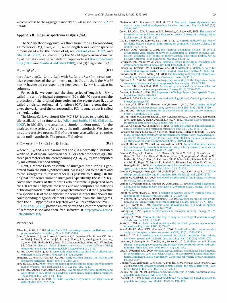

Mode

wd

A

adGCK

�

himc

cpcga

t2aaa

Z

wwtb

etoctooct

ou

R

A

B

B

B

B

B

B

C. Colon et al. / Ecological

hich is close to the aggregate model’s S/K = 0.4; see Section 2.2 foretails.

ppendix B. Singular spectrum analysis (SSA)

The SSA methodology involves three basic steps: (1) embedding time series {X(t) : t = 1, 2, . . ., N} of length N in a vector space ofimension M – for the choice of M, see Vautard et al. (1992) andhil et al. (2002); (2) computing the M × M lag-covariance matrixD of the data – see the two different approaches of Broomhead anding (1986) and Vautard and Ghil (1989); and (3) diagonalizing CD:

D = ETDCDED; (B.1)

ere �D = diag(�1, �2, . . . �M), with �1, �2, . . . �M > 0 the real, pos-tive eigenvalues of the symmetric matrix CD, and ED is the M × M

atrix having the corresponding eigenvectors E� , � = 1, . . . M, as itsolumns.

For each E� we construct the time series of length N − M + 1,alled the �-th principal component (PC); this PC represents therojection of the original time series on the eigenvector E� , alsoalled empirical orthogonal function (EOF). Each eigenvalue ��

ives the variance of the corresponding PC; its square root is called singular value.

The Monte Carlo version of SSA (MC-SSA) is used to reliably iden-ify oscillations in a time series (Allen and Smith, 1989; Ghil et al.,002). In MC-SSA, one assumes a simple, random model for thenalysed time series, referred to as the null hypothesis. We choosen autoregressive process Z(t) of order one, also called a red noise,s the null hypothesis. The process Z(t) solves

(t) = a1[Z(t − 1) − Z0] + �(t) + Z0, (B.2)

here a1, Z0 and � are parameters and is a normally distributedhite noise of mean 0 and variance 1. For each time series X(t), the

hree parameters of the corresponding Z(t ; a1, Z0, �) are computedy maximum-likehood fitting.

Next, a Monte Carlo ensemble of surrogate time series is gen-rated from the null hypothesis and SSA is applied to the data ando the surrogates, to test whether it is possible to distinguish theriginal time series from the surrogates. Specifically, the M × M lag-ovariance matrix of the Monte Carlo ensemble is projected ontohe EOFs of the analysed time series, and one computes the statisticsf the diagonal elements of the projected matrices. If the eigenvaluef a specific EOF of the analysed time series is larger than 95% of theorresponding diagonal elements computed from the surrogates,hen the null hypothesis is rejected with a 95% confidence level.

Ghil et al. (2002) provide an overview and a comprehensive setf references; see also their free software at http://www.atmos.cla.edu/tcd/ssa/.

eferences

llen, M., Smith, L., 1989. Monte Carlo SSA: detecting irregular oscillations in thepresence of coloured noise. J. Clim. 9, 3373–3404.

ale, J.S., Masters, G.J., Hodkinson, I.D., Awmack, C., Bezemer, T.M., Brown, V.K., But-terfield, J., Buse, A., Coulson, J.C., Farrar, J., Good, J.E.G., Harrington, R., Hartley,S., Jones, T.H., Lindroth, R.L., Press, M.C., Symrnioudis, I., Watt, A.D., Whittaker,J.B., 2002. Herbivory in global climate change research: direct effects of risingtemperature on insect herbivores. Glob. Change Biol. 8 (1), 1–16.

arton, D.A.W., Sieber, J., 2013. Systematic experimental exploration of bifurcationswith noninvasive control. Phys. Rev. E 87 (5), 052916.

oettiger, C., Ross, N., Hastings, A., 2013. Early warning signals: the charted anduncharted territories. Theor. Ecol. 6 (3), 255–264.

onabeau, E., 2002. Agent-based modeling: methods and techniques for simulatinghuman systems. Proc. Natl. Acad. Sci. U. S. A. 99, 7280–7287.

oukal, D.S., Sabelis, M.W., Berec, L., 2007. How predator functional responses andAllee effects in prey affect the paradox of enrichment and population collapses.Theor. Popul. Biol. 72 (1), 136–147.

roomhead, D., King, G., 1986. Extracting qualitative dynamics from experimentaldata. Physica D 20, 217–236.

lling 317 (2015) 93–106 105

Chekroun, M.D., Simonnet, E., Ghil, M., 2011. Stochastic climate dynamics: ran-dom attractors and time-dependent invariant measures. Physica D 240 (21),1685–1700.

Crowl, T.A., Crist, T.O., Parmenter, R.R., Belovsky, G., Lugo, A.E., 2008. The spread ofinvasive species and infectious disease as drivers of ecosystem change. Front.Ecol. Environ. 6 (5), 238–246.

Dai, L., Vorselen, D., Korolev, K.S., Gore, J., 2012. Generic indicators for loss ofresilience before a tipping point leading to population collapse. Science 336(6085), 1175–1177.

De Roos, A.M., Persson, L., 2005. Unstructured population models: do generalassumptions yield general theory? In: Cuddington, K., Beisner, B. (Eds.), Eco-logical Paradigms Lost: Routes of Theory Change. Theoretical Ecology Series.Elsevier Academic Press, Burlington, MA, USA, pp. 31–62.

DeAngelis, D.L., Mooij, W.M., 2005. Individual-based modeling of ecological andevolutionary processes. Annu. Rev. Ecol. Evol. Syst. 36 (1), 147–168.

Dhooge, A., Govaerts, W., Kuznetsov, Y.A., 2003. Matcont: a Matlab package fornumerical bifurcation analysis of ODEs. ACM Trans. Math. Softw. 29, 141–164.

Dieckmann, U., Law, R., Metz, J.A.J., 2000. The Geometry of Ecological Interactions:Simplifying Spatial Complexity. Cambridge University Press.

Dijkstra, H.A., Ghil, M., 2005. Low-frequency variability of the large-scale oceancirculation: a dynamical systems approach. Rev. Geophys. 43, RG3002.

Donalson, D.D., Nisbet, R.M., 1999. Population dynamics and spatial scale: effects ofsystem size on population persistence. Ecology 80 (8), 2492–2507.

Durrett, R., Levin, S., 1994. The importance of being discrete (and spatial). Theor.Popul. Biol. 46 (3), 363–394.

Ferrière, R., 2009. Evolutionary Conservation Biology, first ed. Cambridge UniversityPress, Cambridge, UK.

Fussmann, G.F., Ellner, S.P., Shertzer, K.W., Hairston Jr., N.G., 2000. Crossing the Hopfbifurcation in a live predator–prey system. Science 290 (5495), 1358–1360.

Ghil, M., 2001. Hilbert problems for the geosciences in the 21st century. NonlinearProcess. Geophys. 8, 211–222.

Ghil, M., Allen, M.R., Dettinger, M.D., Ide, K., Kondrashov, D., Mann, M.E., Robertson,A.W., Saunders, A., Tian, Y., Varadi, F., Yiou, P., 2002. Advanced spectral methodsfor climatic time series. Rev. Geophys. 40 (1), 3-1–3-41.

Ghil, M., Chekroun, M.D., Simonnet, E., 2008. Climate dynamics and fluid mechanics:natural variability and related uncertainties. Physica D 237, 2111–2126.

González-Olivares, E., González-Yanez, B., Mena-Lorca, J., Ramos-Jiliberto, R., 2006.Modelling the Allee effect: are the different mathematical forms proposed equiv-alents? In: Mondaini, R. (Ed.), Proceedings of the 2006 International Symposiumon Mathematical and Computational Biology BIOMAT 2006.

Gras, R., Devaurs, D., Wozniak, A., Aspinall, A., 2009. An individual-based evolv-ing predator–prey ecosystem simulation using a fuzzy cognitive map as thebehavior model. Artif. Life 15 (4), 423–463.

Grimm, V., Berger, U., Bastiansen, F., Eliassen, S., Ginot, V., Giske, J., Goss-Custard, J.,Grand, T., Heinz, S.K., Huse, G., Huth, A., Jepsen, J.U., Jørgensen, C., Mooij, W.M.,Müller, B., Pe’er, G., Piou, C., Railsback, S.F., Robbins, A.M., Robbins, M.M., Ross-manith, E., Rüger, N., Strand, E., Souissi, S., Stillman, R.A., Vabø, R., Visser, U.,DeAngelis, D.L., 2006. A standard protocol for describing individual-based andagent-based models. Ecol. Model. 198 (1–2), 115–126.

Grimm, V., Berger, U., DeAngelis, D.L., Polhill, J.G., Giske, J., Railsback, S.F., 2010. TheODD protocol: a review and first update. Ecol. Model. 221 (23), 2760–2768.

Grimm, V., Railsback, S.F., 2005. Individual-Based Modeling and Ecology. PrincetonUniversity Press, Princeton.

Grimm, V., Wyszomirski, T., Aikman, D., Uchmanski, J., 1999. Individual-based mod-elling and ecological theory: synthesis of a workshop. Ecol. Model. 115 (2–3),275–282.

Guttal, V., Jayaprakash, C., 2008. Changing skewness: an early warning signal ofregime shifts in ecosystems. Ecol. Lett. 11 (5), 450–460.

Gyllenberg, M., Parvinen, K., Dieckmann, U., 2002. Evolutionary suicide and evolu-tion of dispersal in structured metapopulations. J. Math. Biol. 45 (2), 79–105.

Hale, J.K., Koc ak, H., 1991. Dynamics and Bifurcations. No. 3 in Texts in AppliedMathematics. Springer-Verlag, New York.

Hastings, A., 1990. Spatial heterogeneity and ecological models. Ecology 71 (2),426–428.

Hastings, A., 2004. Transients: the key to long-term ecological understanding?Trends Ecol. Evol. 19 (1), 39–45.

Kantz, H., 1994. A robust method to estimate the maximal Lyapunov exponent of atime series. Phys. Lett. A 185 (1), 77–87.

Kevrekidis, I.G., Gear, C.W., Hummer, G., 2004. Equation-free: the computer-aidedanalysis of complex multiscale systems. AIChE J. 50 (7), 1346–1355.

Kuehn, C., 2011. A mathematical framework for critical transitions: bifurcations,fast-slow systems and stochastic dynamics. Physica D 240 (12), 1020–1035.

Lavergne, S., Mouquet, N., Thuiller, W., Ronce, O., 2010. Biodiversity and climatechange: integrating evolutionary and ecological responses of species and com-munities. Annu. Rev. Ecol. Evol. Syst. 41 (1), 321–350.

Law, R., Dieckmann, U., 2000. Moment approximations of individual-based models.In: Dieckmann, U., Law, R., Metz, J.A. (Eds.), The Geometry of Ecological Interac-tions: Simplifying Spatial Complexity. Cambridge University Press, Cambridge,pp. 252–270.

Lindegren, M., Möllmann, C., Nielsen, A., Brander, K., MacKenzie, B.R., Stenseth, N.C.,2010. Ecological forecasting under climate change: the case of Baltic cod. Proc.

R. Soc. Lond. B: Biol. 277 (1691), 2121–2130.

Loeuille, N., Ghil, M., 1994. Intrinsic and climatic factors in North-American animalpopulation dynamics. BMC Ecol. 4 (6), 12.

Łomnicki, A., 1999. Individual-based models and the individual-based approach topopulation ecology. Ecol. Model. 115 (2–3), 191–198.

1 l Mode

M

M

M

N

P

P

R

R

R

S

S

S

06 C. Colon et al. / Ecologica

ccauley, E., Wilson, W.G., De Roos, A.M., 1993. Dynamics of age-structured andspatially structured predator–prey interactions: individual-based models andpopulation-level formulations. Am. Nat. 142 (3), 412–442.

cQueen, D.J., Johannes, M.R.S., Post, J.R., Stewart, D.J., Lean, D.R.S., 1989. Bottom-up and top-down impacts on freshwater pelagic community structure. Ecol.Monogr. 59 (3).

urdoch, W.W., Kendall, B.E., Nisbet, R.M., Briggs, C.J., McCauley, E., Bolser, R.,2002. Single-species models for many-species food webs. Nature 417 (6888),541–543.

es, E.H.V., Scheffer, M., 2007. Slow recovery from perturbations as a generic indi-cator of a nearby catastrophic shift. Am. Nat. 169 (6), 738–747.

imm, S.L., 1991. The Balance of Nature? University of Chicago Press, Chicago, IL,USA.

imm, S.L., Redfearn, A., 1988. The variability of population densities. Nature 334(6183), 613–614.

Core Team, 2012. R: A Language and Environment for Statistical Computing. RFoundation for Statistical Computing, Vienna, Austria http://www.R-project.org/, ISBN 3-900051-07-0.

ailsback, S.F., Grimm, V., 2011. Agent-Based and Individual-Based Modeling: APractical Introduction. Princeton University Press, Princeton.

eppas, A.I., Tsoumanis, A.C., Siettos, C.I., 2010. Coarse-grained bifurcation analysisand detection of criticalities of an individual-based epidemiological networkmodel with infection control. Appl. Math. Model. 34 (3), 552–560.

cheffer, M., Bascompte, J., Brock, W.A., Brovkin, V., Carpenter, S.R., Dakos, V., Held,H., van Nes, E.H., Rietkerk, M., Sugihara, G., 2009. Early-warning signals forcritical transitions. Nature 461 (7260), 53–59.

chneider, S.H., Dickinson, R.E., 1974. Climate modeling. Rev. Geophys. Space Phys.12, 447–493.

choll, H.J., 2001. Agent-based and system dynamics modeling: a call for cross studyand joint research. In: Proceedings of the 34th Annual Hawaii InternationalConference on System Sciences, Vol. 3, Manui, Hawaii.

lling 317 (2015) 93–106

Schouten, J.C., Takens, F., van den Bleek, C.M., 1994. Maximum-likelihood estimationof the entropy of an attractor. Phys. Rev. E 49 (1), 126–129.

Siekmann, I., 2015. Bifurcation analysis of individual-based models in populationdynamics. Ecol. Complex., 21.

Siettos, C.I., Gear, C.W., Kevrekidis, I.G., 2012. An equation-free approach toagent-based computation: bifurcation analysis and control of stationary states.Europhys. Lett. 99 (4), 48007.

Valladares, F., Matesanz, S., Guilhaumon, F., Araújo, M.B., Balaguer, L., Benito-Garzón,M., Cornwell, W., Gianoli, E., van Kleunen, M., Naya, D.E., Nicotra, A.B., Poorter,H., Zavala, M.A., 2014. The effects of phenotypic plasticity and local adaptationon forecasts of species range shifts under climate change. Ecol. Lett. 17 (11),1351–1364.

van Baalen, M., 2000. Pair approximations for different spatial geometries. In: Dieck-mann, U., Law, R., Metz, J.A. (Eds.), The Geometry of Ecological Interactions:Simplifying Spatial Complexity. Cambridge University Press, Cambridge, pp.359–387.

van Voorn, G.A.K., Hemerik, L., Boer, M.P., Kooi, B.W., 2007. Heteroclinic orbits indi-cate overexploitation in predator–prey systems with a strong Allee effect. Math.Biosci. 209 (2), 451–469.

Vautard, R., Ghil, M., 1989. Singular spectrum analysis in nonlinear dynam-ics, with applications to paleoclimatic time series. Physica D 35,395–424.

Vautard, R., Yiou, P., Ghil, M., 1992. Singular spectrum analysis: a toolkit for shortnoisy chaotic signals. Physica D 58, 95–126.

Walker, B., Holling, C.S., Carpenter, S.R., Kinzig, A., 2004. Resilience, adaptability andtransformability in social-ecological systems. Ecol. Soc. 9 (2), 5.

Wang, J., Shi, J., Wei, J., 2011. Predator–prey system with strong Allee effect in prey.J. Math. Biol. 62 (3), 291–331.

Wilenski, U., 1999. NetLogo. http://ccl.northwestern.edu/netlogo/.Wissel, C., 1984. A universal law of the characteristic return time near thresholds.

Oecologia 65 (1), 101–107.