bibliography and references - home - springer978-1-349-21490-7/1.pdf · bibliography and references...

Bibliography and References

[1) Adey R A (Editor), Parallel Processing in Engineering Applications, Springer-Verlag, Berlin, 1990.

[2] Akl S G, The Design and Analysis of Parallel Algorithms, PrenticeHall, 1989.

[3] Alty J L and Coombs M J, Expert Systems: Concepts and Examples, NCC Publications, 1984.

[4] Artificial Intelligence: An International Journal, Special Volume on Qualitative Reasoning about Physical Systems, Vol 24, Numbers 1-3, Dec 1984.

[5] Astrom K J and Wittenmark B, Computer Controlled Systems: Theory and Design, Prentice-Hall, New Jersey, USA, 1984.

[6] Astrom K J, Anton J J and Arzen K E, Expert Control, Automatica, Vol 22, (3), pp 277-286, 1986.

[7] Ayuk J T, Fault tolerant reconfigurable architectures for flight control, Masters Thesis, University of Sheffield, 1989.

[8] Balas M J, Feedback control of flexible systems, IEEE Transactions on Automatic Control, Vol. AC-23, no. 4, pp. 673-679, 1978.

[9] Balas M J, Enhanced modal control of flexible structures via innovations feedthrough, International Journal of Control, Vol. 32, no. 6, pp. 983-1003, 1980.

[10] Banks S P, Control Systems Engineering, Prentice-Hall, 1986. [11] Barney G C, Intelligent Instrumentation: Microprocessor Applica

tions in Measurement and Control, Prentice-Hall, 1985. [12] Barr A and Feigenbaum E A, The Handbook of Artificial Intelligence,

Vol1, Pitman Books Ltd, 1981. [13] Bennett S, Real-Time Control Systems, Prentice-Hall, 1987. [14] Berg M C, Amit N and Powell J D, Multi-rate Digital Control System

Design, IEEE Trans Aut Control, Vol 33, (12), Dec, pp 1139-1150, 1988.

[15] Bertsekas D P and Tsitsiklis J N, Parallel and Distributed Computation: Numerical Methods, Prentice-Hall, 1989.

169

170 Digital Computer Control Systems

[16] Boy kin W Hand Frazier B D, Multi-rate Sampled-Data Systems Analysis via Vector Operators, IEEE Trans Aut Control, pp 548-551, 1975.

[17) Braae M, and Rutherford D A, Fuzzy relations in a control setting, Tech report Mo 359, control Systems Centre, UMIST, 1977.

[18) Bryson A E and Ho Y C, Applied Optimal Control, Blaisdell, 1969.

[19) Chen C-T, Linear System Theory and Design, Holt, Rinehart and Winston, New York, 1984.

[20) CODAS Operating Manual, Golten and Verwer Parteners, 33 Moseley Rd, Cheadle Hulme, Cheshire.

[21) Concurrency: Practice and Experience, ISSN 1040-3108, John Wiley & Sons Ltd, New York, USA.

[22) Coon G A, How to Find Controller Settings from Process Characteristics, Control Eng, Vol 3 (5), p 66, 1956.

[23) Coon G A, How to Set Three Term Controllers, Control Eng, Vol 3 (6), p 21, 1956.

[24) Davis R, Buchanan B G and Shortliffe E H, Production Systems as a

[25)

[26)

[27)

[28)

[29)

[30)

Representation for a Knowledge-Based Consultation Program, Artificial Intelligence, Vol8, (1), pp 15-45, 1977.

D'Azzo J J and Houpis C H, Linear Control System Analysis and Design: Conventional and Modern, McGraw-Hill, Tokyo, 1981.

DecegamaA L, TheTechnologyofParallelProcessing, Vol1, PrenticeHall, 1989.

Denham M J and Laub A J (Editors), Advanced Computing Concepts and Techniques in Control Engineering, Springer-Verlag, 1988.

Di Stefano III J J, Stubberud A R and Williams I J, Feedback and Control Systems, Schaum's Outline Series, McGraw-Hill, 1967.

Dorf R C, Modern Control Systems, Addison-Wesley, 1986.

Duda R 0, Gaschnig J G and Hart P E, Model Design in the PROSPECTOR Consultation System for Mineral Exploitation, in Ex-pert Systems in the Micro-Electronic Age, Edited by D Mitchie, Edinburgh University Press, pp 153-167, 1979.

[31) Elgerd 0 I, Control Systems Theory, McGraw-Hill, 1967.

[32) Fleming W Hand Rishel R W, Deterministic and Stochastic Control, Springer-Verlag, New York, 1975.

[33) Flowers D C and Hammond J L, Simplification of the Characteristic Equation of Multi-rate Sampled Data Control Systems, IEEE Trans Aut Control, pp 249-251, 1972.

[34) Forgyth R (Editor), Expert Systems: Principles and Case Studies, Chapman and Hall, 1984.

Bibliography and References 171

[35] Franklin G F, Powell J D and Workman M L, Digital Control of Dynamic Systems, 2nd edition, Addison-Wesley, New York, 1990.

[36] Franklin G F, Powell J D and Emami-Naeini A, Feedback Control of Dynamic Systems, Addison-Wesley, New York, 1986.

[37] Franklin M A, Parallel solution of ordinary differential equations, IEEE Trans Computers, C-27 (5), pp 413-430, 1978.

[38] Freeman L and Phillips C (Editors), Applications of Transputers 1, lOS Press, Amsterdam, 1989.

[39] Gehani N and McGettrick A D (Editors), Concurrent Programming, Addison-Wesley, 1988.

[40] Goodwin G C and Sin K S, Adaptive Filtering, Prediction and Control, Prentice-Hall, 1984.

[41] Hayes-Roth F, Waterman D and Lenat D (Editors), Building Expert Systems, Addison-Wesley, 1983.

[42] Hestenes M R, Calculus of Variations and Optimal Control Theory, John Wiley, 1966.

[43] Hoare CAR, Communicating Sequential Processes, Communications of the ACM, 21(8), pp 667-677, 1978.

[44] Hoare C A R and Perrott R H, Operating Systems Techniques, Academic Press, 1972.

[45] Hockney R Wand Jesshope C R, Parallel Computers 2, Adam Hilger, Bristol, 1988.

[46] Houpis CHand Lamont G B, Digital Control Systems, Theory, Hardware, Software, McGraw-Hill, New York, 1985.

[47] lEE Computing and Control Colloquium on, The Transputer: Applications and Case Studies, Digest No 1986/91, 1986.

[48] lEE Computing and Control Colloquium on, Recent Advances in Parallel Processing for Control, Digest No 1988/94, 1988.

[49] lEE Electronics Colloquium on, Transputers for Image Processing Applications, Digest No 1989/22, 1989.

[50] Inman D J, Vibration with control measurement and stability, Prentice-Hall, NJ, 1989.

[51] lnmos Ltd, Communicating Process Architecture, Prentice-Hall, 1988.

[52) Inmos Ltd, occam 2 Reference Manual, Prentice-Hall, 1988.

[53) lnmos Ltd, Transputer Development System, Prentice-Hall, 1988.

[54) lnmos Ltd, Transputer Instruction Set, Prentice-Hall,1988.

[55) Inmos Ltd, Transputer Reference Manual, Prentice-Hall, 1988.

[56) lnmos Ltd, Transputer Technical Notes, Prentice-Hall, 1989.

[57) Jackson P, Introduction to Expert Systems, Addison-Wesley, 1986.


[58] Jones D I, Parallel processing for computer aided design of control systems, Research report, University College of north Wales, 1985.

[59] Jones D I, Occam structures in control, lEE Workshop on parallel processing and control- the transputer and other architectures, Digest 1988/95, 1988.

[60] Journal of Parallel and Distributed Computing, ISSN 0743-7315, Academic Press Inc, San Diego, USA.

[61] Jury E I, Theory and Application of the z-Transform Method, John Wiley, 1964.

[62] Jury E I, A Note on Multi-rate Sampled Data Systems, IEEE Trans Aut Control, pp 319-320, 1967.

[63] Jury E I and Blanchard J, A Stationary Test for Linear Discrete Systems in Table Form, Proc IRE, Vol49, pp 1947-1948, 1961.

[64] Katz P, Digital Control Using Microprocessors, Prentice-Hall, London, 1981.

[65] Kerridge J, occam Programming: A Practical Approach, Blackwell Scientific Publications, Oxford, 1987.

[66] Kickert W J M and van Nauta Lemke H R, Application of a Fuzzy Controller in a Warm Water Plant, Automatica, 12, pp 301-308, 1976.

[67] Krosel S M and Milner E J, Application of integration algorithms in a parallel processing environment for the simulation of jet engines, Proc IEEE Annual Simulation Symposium, pp 121-143, 1982.

[68] Kourmoulis P K, Parallel processing in the simulation and control of flexible beam structure systems, Ph D Thesis, University of Sheffield, 1990.

[69] Kourmoulis P K and Virk G S, Parallel processing in the simulation of flexible structures, lEE Colloquium on recent advances in parallel processing for control, Digest No 1988/94, 1988.

[70] Kuo B C, Digital Control Systems, Holt-Saunders, Tokyo, 1980. [71] Kuo B C, Automatic Control Systems, Prentice-Hall, New Jersey,

1987.

[72] Lapidus L and Seinfeld J H, Numerical Solution of Ordinary Differential Equations, Academic Press, 1971.

[73] Lee E B and Markus L, Foundations of Optimal Control Theory, John Wiley, 1967.

[7 4] Leigh J R, Applied Digital Control (Theory, Design and Implementation), Prentice-Hall, 1985.

[75] Leitch R, Qualitative Modelling of Physical Systems for Knowledge Based Control, in Advanced Computing Concepts and Techniques in Control Engineering, edited by M J Denham and A J Laub, NATO ASI Series, Springer-Verlag, 1988.


(76] Mamdani E H and Assilian S, A Fuzzy Logic Controller for a Dynamic Plant, Int J Man-Machine Studies, 7, pp 1-13, 1975.

(77] Manson G A, The Granularity of Parallelism required in MultiProcessor Systems, in SERC Vacation School on Computer Control, IMC London, 1987.

(78] McDermott J, Rl: An Expert in the Computer Systems Domain, Proc of the AAAI-80, 1, pp 269-271, 1980.

(79] McDermott J, Rl: A Rule-Based Configurer of Computer Systems, Artificial Intelligence, 19, pp 39-88, 1982.

(80] Meirovitch L, Elements of Vibration Analysis, McGraw-Hill, New York, 1986.

(81] Meirovitch L and Oz H, Computational aspects of the control of large flexible structures, Proceedings of the 18th IEEE Conference on Decision and Control, Fort Launderdale, pp. 220-229, 1979.

(82] Meirovitch L and Oz H, Modal-space control of large flexible spacecraft possessing ignorable coordinates, Journal of Guidance and Control, Vol. 3, no. 6, pp. 569-577, 1980.

(83] Mellichamp D A (Editor), Real-Time Computing, Van Nostrand Reinhold Co, New York, 1983.

(84] Michie D (Editor), Introductory Readings in Expert Systems, Gordon and Breach Science Publishers, 1982.

(85] Miranker W L and Liniger W M, Parallel methods for the numerical integration of ordinary differential equations, Math Comp, 21, pp 303-320, 1967.

(86] Newland DE, Mechanical vibration: Analysis and computation, John Wiley & Sons, New York, 1989.

(87] Norman D, Some Observations on Mental Models, in Mental Models, edited by D Gentner and L A Stevens, Lawerence Earlbaum Associates, 1983.

(88] Ogata K, Modern Control Engineering, Prentice-Hall, New Jersey, 1970.

(89] Ogata K, Discrete-Time Control Systems, Prentice-Hall, New Jersey, 1987.

(90] Owens D H, Multivariable and Optimal Systems, Academic Press, 1981.

(91] Papoulis A, Probability, Random Variables, and Stochastic Processes, McGraw-Hill, 1965.

(92] Parallel Computing, ISSN 0167-8191, North Holland, Amsterdam, Netherlands.

[93] PC-MATLAB User Guide, The MathWorks Inc, 20 North Main Street, Suite 250, Sherborn, MA 01770, USA.


[94] Phillips C L and Harbor R D, Feedback Control Systems, PrenticeHall, New Jersey, 1988.

[95] Pontryagin E F, Boltanskii V G, Gamkrelidze R V and Mishchenko [E F ,] The Mathematical Theory of Optimal Processes, Pergamon Press, 1964.

[96] Pritchard D J and Scott C J (Editors), Applications of Transputers 2, lOS Press, Amsterdam, 1990.

[97] Raible R H, A Simplification of Jury's Tabular Form, lEE Trans on Automatic Control, Vol AC-19, pp 248-250, 1974.

[98] Raven F H, Automatic Control Engineering, McGraw-Hill, 1978. [99] Rutherford D and Carter G A, A Heuristic Adaptive Controller for a

Sinter Plant, Proc 2nd IFAC Symp Automation in Mining, Mineral and Metal Processing, Johannesburg, 1976.

[100] Shannon C E, Oliver B M and Pierce J R, The Philosophy of Pulse Code Modulation, Proc IRE, Vol 36, pp 1324-1331, 1948.

[101] Shannon C E and Weaver W, The Mathematical Theory of Communication, University of Illinois Press, 1972.

[102] Sharp J A, An Introduction to Distributed and Parallel Processing, Blackwell Scientific Publications, 1987.

[103] Shortliffe E H, Computer Based Medical Consultation: MYCIN, American Elsevier, New York, 1976.

[104] Stallings W, Computer organisation and architectures, Macmillan, New York, USA, 1987.

[105] Sugeno M (Editor), Industrial Applications of Fuzzy Control, NorthHolland, 1985.

[106] Sutton R and Towill D R, An introduction to the use of fuzzy sets in the implementation of control algorithms, Jour Inst Elect and Radio Eng, Vol 55, No 10, pp 357-367, 1985.

[107] Timoshenko S, Young D H, and Weaver W, Vibration Problems in Engineering, John Wiley & Sons, New York, 1974.

[108] Thomson W T, Theory of vibrations with applications, 3rd ed, Prentice Hall Englewood Cliffs, NJ, 1988.

[109] Tong R M, A Control Engineering Review of Fuzzy Systems, Automatica, Vol13, pp 559-569, 1977.

[110] Treu S, Interactive Command Language Design Based on Required Mental Work, Int J Man-Machine Studies, Vol 7, (1), pp 135-149, 1975.

[111] Tse F S, Morse IE and Hinkle R T, Mechanical vibrations, Allyn and Bacon Inc, Boston, 1978.

[112] Van de Vegte J, Feedback Control Systems, Prentice-Hall, New Jersey, 1986.


(113] Van der Rhee F, Van Nauta Lemke and Dijkman J G, Knowledge based fuzzy control of systems, IEEE Trans on Aut Control, Vol 35, No 2, 1990.

(114] Virk G S, Algorithms for State Constrained Control Problems with Delay, Ph D Thesis, Imperial College, University of London, 1982.

(115] Wadsworth C, Who Should Think Parallel ? SERC/DTI Transputer Initiative, Mailshot, Sept 1989.

[116] Warwick K, Control Systems: An Introduction, Prentice-Hall, 1989.

[117] Wiberg D M, State-space and Linear Systems, Schaum's Outline Series, McGraw-Hill, 1971.

[118] Young R M, The Machine Inside the Machine: Users' Models of Pocket Calculators, Int J Man-Machine Studies, 15, pp 15-83, 1981.

[119] YoungS J, An Introduction to ADA, Ellis Horwood Publishers, 1983.

[120] Zadeh L A, Fuzzy Sets, Information and Control, Vol 8, pp 338-353, 1965.

[121] Zadeh L A, Outline of a new approach to the analysis of complex systems and decision processes, IEEE Trans on Systems, Man and Cybernetics, SMC-3, No 1, pp 28-44, 1973.

[122] Zadeh L A, Making Computers Think Like People, IEEE Spectrum, pp 26-32, 1984.

[123] Ziegler J G and Nichols N B, Optimum Settings for Automatic Controllers, Trans ASME, Vol 64, pp 759-768, 1942.

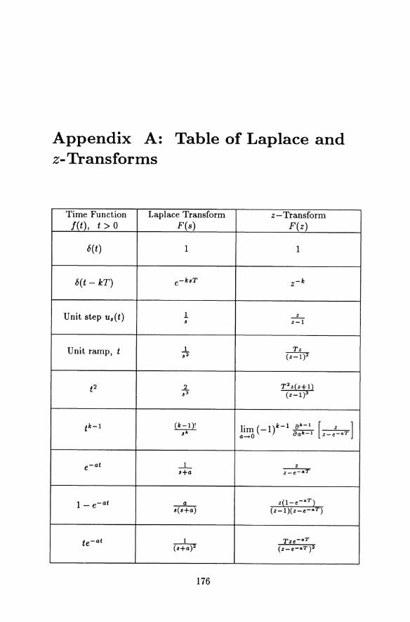
Appendix A: Table of Laplace and z-Transforms

Time Function Laplace Transform z-Transform f(t), t > 0 F(s) F(z)

6( t) 1 1

t5(t- kT) e-bT z-k

Unit step u,(t) 1 _z_ • z-1

Unit ramp, t 1 Tz ..,. (z-1 )2

t2 2 T 2 z(z+1) .3 (z-1)3

tk-1 (k-1)! lim ( -1)k-1 &k-l [-z-] .k a-+0 &ak-l z-e-•T

e-at _1_ z •+a z-e-aT

1- e-at a z(l-e-•T) •(•+a) (z-1)(z-e-•T)

te-at 1 Tze-aT (•+a)2 (z-e-•T) 2

176

Table of Laplace and z-Transforms 177

Time Function Laplace Transform z-Transform f(t), t > 0 F(s) F(z)

tke-at ~ (-1)k ::k [z-ez-aT] (•+a)k

_1_ (e-at_ e-bt) 1 1 [z-ez-aT - z-ez-bT] (b-a) (•+a)(•+b) (b-a)

be-bt - ae-at (b-a)• z[z(b-a)-(be-aT -ae-bT)] (•+a)(•+b) (z-e aT)(z-e bT)

t - ~ (1 -e-at) a Tz - (1-e-aT)z •2(•+a) (z-1)2 a(z-1)(z-e aT)

(1- at) e-at • z[z-e-aT(1+aT)] (•+a)> (z-e aT)2

1- e-at (1 +at) a2 z[za+/1] •(•+a)2 (z-1)(z-e-aT)2

a=l-e-aT -aTe-aT

f1=e-2aT -e-aT +aTe-aT

te-at 1 Tze-aT (•+a)2 (z-e aT)2

sinwt w z sinwT •2+w2 z2-2zcoswT+1

coswt • z(z-coswT} •>+w2 z>-2zcoswT+1

e-at sinwt w ze-aT sinwT (•+a)2+w2 z2-2ze aT coswT+e-2«T

e-at coswt •+a z2-ze-aT coswT (•+a)~+w 2 z2-2ze-«T coswT+e- 2aT

Appendix B: Continuous Second-order Systems

B.l Introduction

In this appendix we present results relating to continuous second-order systems since they are used widely in conventional control systems design where dominant second-order behaviour can be assumed for higher-order systems. We will assume a transfer function of the following standard form

(B.1)

where ( is defined to be the dimensionless damping ratio, and Wn is the undamped natural frequency (see Phillips and Harbor [94]; D' Azzo and Houpis [25]; Ogata [88]). Note that the DC gain of the system is unity. The response of this system to a unit step input, subject to zero initial conditions can be shown (see D'Azzo and Houpis [25] ) to be given by

e-(w,.t ( ) y (t) = 1- v'1=(2 sin Wn v'1=(2t + cos- 1 (

1- (2 (B.2)

A family of curves representing the step responses is shown in Figure B.1, where the horizontal axis is the dimensionless variable wnt. The curves are thus functions only of the damping ratio and show that the overshoot is dependent upon(; for overdamped and critically damped cases ( ~ 1, there is no overshoot and no oscillation; for underdamped cases, 0 ~ ( < 1, the system oscillates around the final steady-state value. The peak overshoot as ( varies is shown more clearly in Figure B.2.

B.2 Response Specifications

Before a control system is designed, specifications must be developed that describe the characteristics that the system should possess. Some of these

178

Continuous Second-order Systems 179

y(t)

Figure B.l Step responses for second-order systems

100

80

0 60 0 .r:: .e! Q) > 0

E 40 Q)

~ Q)

c...

20

0 0.2 0.4 0.6 0.8 1.0

Damping ratio I;;

Figure B.2 Peak overshoot versus damping ratio

180

Output y MP

0.1

Digital Computer Control Systems

____________ j ________ _ ....__ __ .-_ ..... _ ..... __________ ~1

...... _ ------..... _ --_:-_-:_-_ Yss

Error tolerance band

Time/seconds

t,

Figure B.3 Unit step response of a system

can be written in terms of the system's step response. A typical step response of a second-order system is shown in Figure B.3. Some characteristics that can be used to describe the response include the following.

(i) The rise time, tr, is the time taken for the response to rise from 10% of the final value to 90% of the final value.

(ii) The peak value of the step response is denoted by Mp, and the time to reach this peak value is tp.

(iii) The percentage overshoot is defined by

Mp -Yu Percentage overshoot= X 100% (B.3) Yu

where y$$ is the final or steady-state value of the output y(t). (iv) The settling time, t$, is the time required for the output to settle

within a certain percentage of its final value. Commonly used values for the error-band are 2% or 5%. For second-order systems, the value of the transient component at any time is equal to or less than the exponential e-(w,.t. The settling times expressed in a number of time constants r for different error bands are given in Table B.l.

(v) The delay time, td, is the time required for the response to reach half the final value the very first time.

We have defined the above parameters for the underdamped case; tr, t$, Yu and td are equally meaningful for the overdamped case, but Mp, tp and percentage overshoot obviously have no clear meaning in these cases.

20

10

dB -10

-20

-30

deg. -1

Continuous Second-order Systems

s=o.5 s=o.6

s=o.8 s=1.o

Second-order system amplitude ratio

0.2 0.3 0.4 0.5 0.6 0.8 1 w

Second-order system phase shift

w

2

181

3 4 5 6 7 8 910

Figure B.4 Frequency response curves for second-order systems


Table B.l Settling times for various error bands

Error Settling time I band,% t,, seconds

10 2.3T 5 3.0T 2 3.9T 1 4.6T

B.3 Frequency Response Characteristics

Control system specifications can also be described in frequency domain terms. Considering the standard second-order system:

G(s)

(B.4)

the frequency domain analysis can be performed by letting s = jw so that we have

G(jw) = 21

[1- (:~) ] + j2( (:~) (B.5)

For this transfer function we define normalised frequency w1 = w / Wn. The gain and phase curves for various values of ( are given in Figure B.4 where the gain in decibels (dB) is defined as

dB= 20 log10(Numeric Gain) (B.6)

For a constant (, increasing Wn causes the bandwidth (the frequency range over which the gain is greater than 0 dB), to increase by the same factor. It can be shown (see Phillips and Harbor [94]) that

(B.7)

Hence for constant (, increasing Wn decreases tp and tr by the same factor. This result can be approximately applied to general systems and not just to second-order ones. The reason for this is that higher-order systems can be approximated by their dominant (second-order) modes.

In the frequency domain we design for concepts such as gain margins and phase margins. These are defined as follows:

Continuous Second-order Systems 183

Gain Margin

If the magnitude of the open-loop function of a stable closed-loop system at the 180° phase crossover on the frequency response diagram (Nyquist, Bode, etc.) is the value a, the gain margin is 1/a, and is usually expressed in decibels.

Phase Margin

The phase margin is the magnitude of the angle (180°- phase angle) at the point when the open-loop system gain is unity (0 dB).

The phase margin can be obtained for the standard second-order system as a function of damping ratio (and plotted as shown in Figure B.5.

100

80

til CD ~ 60 c: -~ Ill E CD II) Ill 40 .s:::. a.

20

0 0.2 0.4 0.6 0.8 1.0

Damping ratio ~

Figure B.5 Phase margin versus damping ratio

As can be seen, the lower end of the graph can be approximated reasonably by the linear relationship

Phase Margin~ 0.~ 1 (B.8)

Appendix C: The Transputer and occam

C.l Introduction

The general concepts of parallel processing have been discussed in chapter 6 and it is the intention here to concentrate on how such systems can be implemented using transputer technology. The transputer is a VLSI device which comprises a processor, memory and external communication links on a single substrate of silicon. It has been designed by Inmos Ltd to be used as a programmable component in implementing parallel processing systems. In view of this, the word "transputer" has been derived from TRANSistor (a single component that can be used in conjunction with others in electronic circuits), and comPUTER (a machine whose main task

\

Onchip ~ CPU memory \ ....,

I Timers I Link 0

Link 1

L External Link 2 w memory ....>.

interface Link 3 \

Event

Figure C.l Structure of the transputer

0

1

2

3

E xternal links

Event link

is processing information/data quickly and efficiently). The basic structure of the transputer is shown in Figure C.1, although there are variations on this to form a family of devices. Transputers come in 16 and 32 bit wordlength versions; some have a hardware floating point unit, while others can have disk storage device controllers on chip. The amount of memory and

184

The Transputer and occam 185

number of links can vary as well as the processing speeds (see Inmos [51] -[56]).

Hence, although a transputer is essentially a computer on a single chip, and can be used as such (with suitable 1/0), its unique external links allow other transputers to be connected to it. In this way transputer array systems can be constructed and used in a variety of applications, see lEE Computing and Control Colloquiums [47], [48]; lEE Electronics Colloquium [49]; Freeman and Phillips [38]; Pritchard and Scott [96]. The links allow serial point-to-point communication to take place between processors and thus avoid the bus contention problems in conventional shared memory data-bus computer systems, as discussed in chapter 6. A link can operate at 5, 10, or 20 Mbits per second in both directions at the same time. These speeds are likely to increase with future generations of transputers. Once a link communication has been initiated by the processor, it proceeds autonomously allowing the processor to execute another process.

External interrupt requests can be received on a separate link, called the event link, which is handled in a similar fashion to the communication links. At present there is no support for the prioritisation of interrupt requests and all such matters must be handled explicitly by the system designer. Future transputers are likely to have more event pins, thus allowing for multi-level interrupt structures.

Figure C.2 occam process model

C.2 occam Overview

The model of concurrency supported in hardware by transputers is the occam model, which has the following features:

(i) The world is made up of processes which exist in parallel, that is, at the same time.


(ii) Processes may be born and may die. (iii) Processes may spawn other processes. (iv) Processes can communicate between each other using messages through

channels. (v) A channel is a uni-directional, unbuffered link between just two pro-

cesses. (vi) A channel provides synchronised communication.

(vii) A process is either a primitive process or a collection of processes. (viii) A collection specifies both its extent (what processes are in the col-

lection), and how the collection behaves.

A typical occam process model is shown in Figure C.2, where such parallel processes are clearly shown, and how they can interact with each other via one way channels.

Process P1 is a primitive process which interacts with processes P2 and Pa, by sending messages to P2 (via channel C12) and Pa (via channel C1a), while receiving messages only from P2 (via channel C21). Process P2 is a collection of communicating processes P21 and P22, etc.

Some precise details of occam are now given to illustrate the language; full details can be found in the occam 2 reference manual, [52]. All processes in occam are constructed using three primitive processes, namely:

(i) assignment, when an expression is computed and the result assigned to a variable as in

:z: := 20

so that ":z:" is set to 20; (ii) input, for when a message is received on a communication channel;

the "?" mark is used to indicate input and so

In ? :z:

sets the variable ":z:" to the value input from the channel "In"; (iii) output, for when a message needs to be sent to another process. The

"!" mark is used to indicate output on a specified channel, and so

Out! :z:

ouputs the value ":z:" on the channel "Out".

Using these three instructions together with the following constructors, more complex processes can be formed. occam uses indentations from the lefthand edge of the page to define the structure of the processes, as will become clear from the following discussion.


SEQ: The sequence constructor defines a process whose component processes are executed in order, terminating when the last process ends, for example:

SEQ In? x y :=X* X

Out! y PAR: The parallel constructor defines a process whose component processes

are executed concurrently. This process terminates when all of the constituent process have ended, for example:

PAR Out1! a Out2! b

ALT: The alternative constructor defines a process encompassing other processes which have an input as their first component. The first process to become ready is executed. The ALT process terminates when the chosen process terminates, for example:

ALT In1? x

Out1 ! x In2? x

Out2! x IF: The condition constructor defines a process, each component of which

has a condition as its first component. If a condition is found to be satisfied (that is, TRUE) then that process is executed. The condition process terminates when that process terminates, for example:

IF X<> 0

x:= x + 10 x=O

SKIP

WHILE: The repetition constructor defines a condition and a process which will be repeatedly executed until a false condition is evaluated, for example:

WHILE x <> 0 SEQ

In? x Out! x

In addition, all of the above constructors can be repeated for a known number of times, for example:

SEQ i = 0 FOR 6

188

SEQ In? x Out! x


will input "x" on channel "In", and output "x" on channel "Out" 6 times. The channels are defined in the same way as variables, for example:

CHAN OF INT In:

CHAN OF ANY In:

defines the channel "In" to accept variable integer values.

allows the channel "In" to accept any type of variable integer, real, or byte.

To enable abstraction, a name can be given to the text of a process, for example:

PROC SQU(CHAN OF REAL In, Out) REAL16 x: SEQ

In? x Out! x * x

Using these constructs, concurrent programs can be written in a straightforward manner. The occam channels provide synchronised communication between two concurrent processes. Hence data is transferred only when the two processes are ready.

lnmos have provided an occam programming environment under the "Transputer Development System" (TDS) where a folding editor is used. Three dots at the start of a line indicate that information is folded away (hidden from view). In this way a hierarchy of folds can be created so that the program has structure and the different levels can be investigated by entering or exiting from folds.

The TDS environment also provides various utilities such as a compiler and configurer. A full description of the facilities can be found in the TDS user guide [53).

C.3 Transputer Systems and occam Configuration

As already mentioned, the transputer has been designed to implement the occam model of concurrency efficiently. Figure C.3 shows a typical transputer system model, showing three transputers communicating through the external links. As shown, this system can be used to implement the occam process model of Figure C.2 in a straightforward way by mapping process P1 to transputer 1, etc.

A transputer has its own scheduler and so it can be used to run a number of concurrent processes together by time-sharing the processor. Also, the

The Transputer and occam

Transputer link

T"'"i"'e' @

Link

Link

Figure C.3 Transputer system model

Transputer 3

189

communication channels between processes can be through the external hardware links on the transputers or internal software channels by using memory locations. Each transputer link provides two occam channels; one channel is an input channel, and the other an output channel. Both have to be specified in the program.

The external link channels between transputers and the internal software channels on one transputer are seen to be identical at run-time. Therefore it is possible to develop a solution to a problem independently of the actual transputer network upon which it will be executed. For instance the solution can be developed on a single transputer, and once the solution is functional, the various processes can be allocated to different transputers, and the channels allocated to the links of the appropriate transputers for final implementation. The occam configuration facilities that allows such allocations are as follows:

PLACED PAR:

This is similar to the ordinary PAR statement except that the processes are to be placed on separate transputers.

PROCESSOR number transputer. type:

This is used to identify a number to a processor and what transputer. type the processor is, so that the configurer can check that the correct compiler was used, that is, T2 or T212 for the T212, T222, T225 or M212 16-bit transputers, T4 or T414 for the T414 32-bit transputer, T425 for the T425 32-bit transputer and T8 or T800 for the T800, T801 or T805 32-bit floating point transputers.


PLACE channel. name AT link. address:

This provides a means of allocating a channel identified as channel. name to a particular transputer link identified by link. address. The link. address also identifies whether the channel is a source or destination by the following method: the four links on, say, a T414 transputer give rise to 8 occam channels (4 input and 4 output channels). Link 0 gives channels 0 and 4, Link 1 gives channels 1 and 5 etc., where 0,1,2,3 are output channels and 4,5,6 7 are input channels.

Further details are given in the TDS user guide, [53] and the occam 2 reference manual [52].

Therefore transputers and occam are ideally suited to each other, and in fact lnmos originally intended all transputer programming to be performed in occam. A claim made by Inmos is that the occam compiler produces almost optimal executable code which can only be marginally improved by an expert assembly language programmer. An average assembly language programmer would produce worse code than the compiler. In spite of this claim, which appears to be supported by many computer scientists, there has been a strong resistance to occam from the application user community because it is a new language which has to be learnt and implemented. Many millions of man years have been spent on writing programs in a variety of languages - for these to be run on transputer systems would require major re-writing and expenditure. Therefore, the majority of users required new compilers to support their normal programming languages on transputer hardware so that their existing codes could be executed on transputers. In the light of these demands, several high level language compilers for transputers have been developed, and are now available. Parallel extensions to the sequential languages have also been inserted to give parallel versions of the languages. It is now possible to program multi-transputer systems in Fortran, C, Pascal, etc. Software tools to assist users in programming and debugging parallel computer systems are also emerging.

We now present an example which will illustrate the parallel programming approach using transputers and occam.

C.4 Vibration Control of a Flexible Cantilever

The example we will consider is that of vibration suppression in a flexible cantilever system. Problems of vibration are common in engineering applications and there is a clear need for these problems to be studied so that effective control/vibration suppression techniques can be developed and implemented. Examples of where such oscillatory behaviour occurs include aircraft fuselage and wings, satellite solar panels and buildings. The problems stem mainly from the use of lightweight designs aimed at improving performance and/or reducing costs, but which also lead to vibrational


difficulties. The main methods for handling the unwanted vibrations are:

(i) to introduce passive damping elements such as springs and/or dampers, (ii) to use active control techniques to provide the damping actively when

required, or (iii) a combination of the two techniques.

We will use the active damping method to address and computer-control, in real-time, the vibrational problems encountered in a flexible beam structure. We shall concentrate on a cantilever system which can represent, for example, vibrations in aircraft wings and/or the swaying of tall skyscrapers in windy conditions. Other applications can be considered by changing the boundary conditions on the beam - for example free-free beams can be used to represent aircraft fuselage oscillations and hinged-free beams for satellite solar panel oscillations. Clearly the simple beam system will not include all the two- and three-dimensional vibrational effects, but it does represent a first attempt for the consideration of several practical applications.

y(x,t)

X

Figure C.4 Cantilever system in transverse vibration

A cantilever system in transverse oscillation (see Figure C.4) has its motion described by the fourth-order partial differential equation (PDE), see for example Timoshenko et al. [107],

(C.1)

where y(x, t) is the deflection at a distance x from the fixed end at timet, p. is a beam constant and f(x, t) is a force causing the beam to deform. It is well known that flexible structure systems such as those described by equation (C.1) have an infinite number of modes, see Meirovitch [80], Newland [86], Thomson [108] and Tse et al. [111], although in most cases the lower order modes are the dominant ones which need consideration. Higher modes have little effect in this beam system and can be ignored in much of the analysis, see Kourmoulis [68]. However what is a low mode and what is a


high mode is a subjective decision, although it is clear that as more modes are considered in the analysis, the better is the performance that one can expect. Such an increase in dimensionality leads to requiring vast computing resources so that the real-time processing demands are satisfied, for the modelling and controller design and implementation. In fact the computing demands can get so enormous in practice that they are difficult to satisfy using sequential computing methods. Therefore parallel processing methods using transputer hardware, as considered here, can be more appropriate.

The approach taken here follows along the lines outlined in chapter 6 where the overall computing task is divided into the following main subtasks:

(a) System simulation (necessary if the actual system is unavailable, does not exist or for testing of the modelling and controller designs).

(b) Controller design, implementation and assessment. (c) Modelling (generally reduced order) for state estimation and valida

tion. (d) User interface. Disturbance-------~

forces

P, Controller

design and implementation

User interface

Output deflections

Figure C.5 occam process model for cantilever control

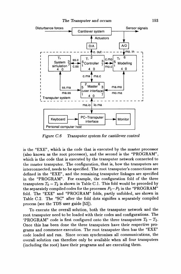
These sub-tasks can be treated as separate occam processes which interact with each other to give the overall solution. One such design can be as shown in Figure C.5. An obvious approach for solving the problem is where the three processes Po - P2 are mapped onto three transputers as shown in Figure C.6, together with a master processor which controls the overall computations and performs the user interface through a personal computer.

In programming multi-transputer systems of this kind using the TDS, there are two sections of code that need to be written. The first of these


Disturbance forces

To System 3

simulation 7 4 0

c.ss

2 6 ss.ma 5 Master 3 ma.mo ma.ss (user interface)~----'

Sensor signals

1 4 0 7 mo.ma ~ ~a~!~te_: ~s~e~ _ _ _ _ _ _ _ _ _ _ _ _______ J

ma.io io.ma

PC-Transputer interface

Figure C.6 Transputer system for cantilever control

193

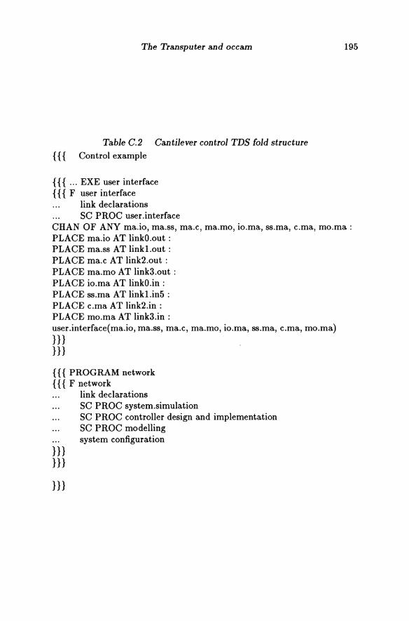
is the "EXE", which is the code that is executed by the master processor (also known as the root processor), and the second is the "PROGRAM", which is the code that is executed by the transputer network connected to the master transputer. The configuration, that is, how the transputers are interconnected, needs to be specified. The root transputer's connections are defined in the "EXE", and the remaining transputer linkages are specified in the "PROGRAM". For example, the configuration fold of the three transputers To- T2 is shown in Table C.l. This fold would be preceded by the separately compiled codes for the processes Po- P2 in the "PROGRAM" fold. The "EXE" and "PROGRAM" folds, partly unfolded, are shown in Table C.2. The "SC" after the fold dots signifies a separately compiled process (see the TDS user guide [53]).

To execute the overall solution, both the transputer network and the root transputer need to be loaded with their codes and configurations. The 'PROGRAM" code is first configured onto the three transputers To- T2. Once this has been done the three transputers have their respective programs and commence execution. The root transputer then has the "EXE" code loaded and run. Since occam synchronises all communications, the overall solution can therefore only be available when all four transputers (including the root) have their programs and are executing them.


Table C.l Transputer configuration fold { { { System Configuration VAL linkO.out IS 0: VAL linkO.in IS 4: VAL linkl.out IS 1: VAL linkl.in IS 5: VAL link2.out IS 2: VAL link2.in IS 6: VAL link3.out IS 3: VAL link3.in IS 7:

CHAN OF ANY mo.in, c.out, ss.c, c.ss, c.mo, mo.c, c.ma: CHAN OF ANY ma.c, ss.ma, ma.ss, ma.mo, mo.ma, ma.io, io.ma :

PLACED PAR PROCESSOR 0 T8

PLACE ss.ma AT linkO.out : PLACE ss.c AT link3.out : PLACE ma.ss AT linkO.in: PLACE c.ss AT link3.in: system.simulation(ss.ma, ss.c, ma.ss, c.ss)

PROCESSOR 1 T8 PLACE c.ma AT linkO.out : PLACE c.ss AT linkl.out : PLACE c.out AT link2.out: PLACE c.mo AT link3.out : PLACE ma.c AT linkO.in: PLACE ss.c AT linkl.in : PLACE mo.c AT link3.in : controller(c.ma, c.ss, c.out, c.mo, ma.c, ss.c, mo.c)

PROCESSOR 2 T8

}}}

PLACE mo.ma AT linkO.out : PLACE mo.c AT linkl.out: PLACE ma.mo AT linkO.in: PLACE c.mo AT linkl.in : PLACE mo.in AT link2.in : modelling(mo.ma, mo.c, ma.mo, c.mo, mo.in)


Table C.2 Cantilever control TDS fold structure { { { Control example

{{ { ... EXE user interface { { { F user interface

link declarations SC PROC user .interface

195

CHAN OF ANY ma.io, ma.ss, ma.c, ma.mo, io.ma, ss.ma, c.ma, mo.ma : PLACE ma.io AT linkO.out : PLACE ma.ss AT linkl.out : PLACE ma.c AT link2.out : PLACE ma.mo AT link3.out : PLACE io.ma AT linkO.in : PLACE ss.ma AT linkl.in5 : PLACE c.ma AT link2.in : PLACE mo.ma AT link3.in: user.interface(ma.io, ma.ss, ma.c, ma.mo, io.ma, ss.ma, c.ma, mo.ma) }}} }}}

{ { { PROGRAM network { { { F network

}}} }}}

}}}

link declarations SC PROC system.simulation SC PROC controller design and implementation SC PROC modelling system configuration


In this way a large complex computational problem can be broken down into smaller subproblems which can be solved on a network of transputers in an efficient manner. Kourmoulis [68] presents real-time simulation results for this cantilever control example where the system simulation, modelling, controller design and user interface sub-tasks are solved on tailormade transputer architectures. The complete network is shown in Figure C.7, and consists of 17 T800 and 2 T414 transputers.

: Sytem 1 simulation : '- --------------

Modelling

1- --- - -- - - - - - - ..,

I I I I I C I I p 1

I I ! ____________ _!

Figure C. 7 Overall transputer network system

A short description of each block is necessary to appreciate the approach; a fuller discussion can be found in Kourmoulis [68].

System Simulation

To simulate the cantilever system, the PDE in equation (C.l) can be numerically solved using finite difference approximations in time and space.


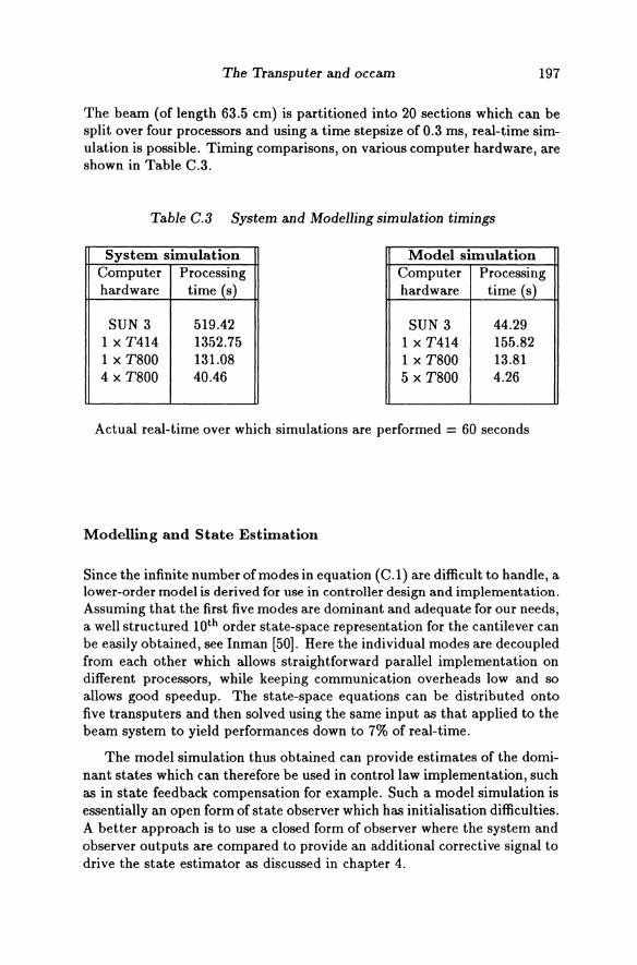
The beam (of length 63.5 em) is partitioned into 20 sections which can be split over four processors and using a time stepsize of 0.3 ms, real-time simulation is possible. Timing comparisons, on various computer hardware, are shown in Table C.3.

Table C.3 System and Modelling simulation timings

System simulation Model simulation Computer Processing Computer Processing hardware time (s) hardware time (s)

SUN 3 519.42 SUN 3 44.29 1 X T414 1352.75 1 X T414 155.82 1 x T800 131.08 1 x T800 13.81 4 X T800 40.46 5 X T800 4.26

Actual real-time over which simulations are performed = 60 seconds

Modelling and State Estimation

Since the infinite number of modes in equation (C.1) are difficult to handle, a lower-order model is derived for use in controller design and implementation. Assuming that the first five modes are dominant and adequate for our needs, a well structured lOth order state-space representation for the cantilever can be easily obtained, see Inman [50]. Here the individual modes are decoupled from each other which allows straightforward parallel implementation on different processors, while keeping communication overheads low and so allows good speedup. The state-space equations can be distributed onto five transputers and then solved using the same input as that applied to the beam system to yield performances down to 7% of real-time.

The model simulation thus obtained can provide estimates of the dominant states which can therefore be used in control law implementation, such as in state feedback compensation for example. Such a model simulation is essentially an open form of state observer which has initialisation difficulties. A better approach is to use a closed form of observer where the system and observer outputs are compared to provide an additional corrective signal to drive the state estimator as discussed in chapter 4.


Controller Design

The beam system PDE of equation (C.l) has zero damping hence any disturbance will set it into continual oscillation. This is clearly not a desirable situation and damping needs to be inserted using a suitable controller. Many methods can be used for the controller design such as pole-placement, PID, dead-beat and optimal control. The approach taken here is to use state feedback (see Kourmoulis [68]) to introduce critical damping to each of the decoupled modes considered, leaving the natural frequencies unchanged. A controller is designed for the lOth_order model and applied to both the model and the system simulation blocks on-line. Figure C.8 shows a typical response of the model and system simulation blocks under state feedback when a disturbing step force is applied. Table C.4 shows the overall timing performance of the system shown in Figure C.7 as well as timings for other hardware implementations.

~~ \ System output 2.0r

0.0 r-----+--r---r-----t---11~_.,...---;--~--tr t(s) 20

-1.0

(em) \ Model output 2.0~

0.0 ~---t----t--+---t-----i~c--lo..--t----;----+---;1 t(s) 20

-1.0

System and model outputs

(om) \ 2.0~ 0.0 ----i---+--+---+---~t--"""--+-1 --t---r--t----tr t(s)

20 -1.0

'} (em)

0.0 e I

-0.5 r Error

1 t(s) 20

Figure C.B State feedback control results of cantilever system


Table C.4 Timings of vibration control transputer system

Network Processing Time (s)

Actual time of SUN 3 1 x T414 1 X T800 17 X T800 simulation (s) 2 X T414

1.0 26.44 81.96 7.55 0.68 30.0 793.29 2538.53 214.4 18.97 60.0 1586.57 5235.68 453.31 40.82

User Interface

In most control applications, it is useful to have a graphics screen to display the performance of the system. In this respect such a display was developed and included the ability to display the deflection of any point along the beam with time, error displays and real-time animation of the beam.

Appendix D: Solutions to Problems

Chapter 2

1. (i) For u (t) = 1, t ~ 0

U (z) 1 + z- 1 + z-2 + z-3 + ... z

z-1

(ii) For u (t) = e-at, t ~ 0

z = z- e-aT

(iii) For u (t) = sin wt, t ~ 0

U (z) sinwTz- 1 +sin 2wTz-2 +sin 3wTz-3 + · · · zsinwT

z2 - 2z cos wT + 1

(iv) For u (t) = coswt, t ~ 0

U (z) = 1 + coswTz- 1 + cos2wTz-2 + cos3wTz-3 + · · ·

z2 - zcoswT z2- 2zcoswT+ 1

2. (i) y (kT) = 1.333- 1.333 ( -0.5)A:, for k = 0, 1, 2, 3, ....

(") (kT) __ -2 (0.707j)A: fork odd } r k _ O 1 2 3 11 y O r k tOr - , , , , .... tor even (iii) y(kT) = 2- 2(-1)k, fork= 0, 1,2,3, .... (iv) y (kT) = 6.62-14.65 (0.734)A: +7.5 (0.614)A:, fork= 0, 1, 2, 3, ....

3. The closed-loop transfer function is

Y(z) _ KT U (z) z- (1- KT)

200

Solutions to Problems

For/{ = 1, and unit step input

y(kT)=1-(1-Tl, fork=0,1,2,3, ...

Hence the output depends on the sampling interval T. T= 0.25 s

201

y (kT) = 1- (0.75)k, for k = 0, 1, 2, 3, ... which gives an overdamped response. This holds for T = 0.25 - 1-.

T= 1 s y (kT) = 1, for k = 1, 2, 3, ... which gives a deadbeat response. As T is further increased the system becomes underdamped.

T = 1.5 s y (kT) = 1- (-0.5)k, fork= 0, 1, 2, 3, ... , which gives an oscillatory response. As T is further increased the oscillations become larger as the damping is reduced.

T= 2 s y (kT) = 1- ( -1)k, for k = 0, 1, 2, 3, ... , which gives continual oscillations. The system is critically stable at this point. As T is further increased the system goes unstable. For example, consider:

T= 3 s y (kT) = 1- ( -2)k, for k = 0, 1, 2, 3, ... , which gives oscillations that grow in magnitude.

4. The limiting values are I< ~ 9 and T ~ 0.26 s.

5. (i) The z-transform of the output is

y (z) = 0.0049834z + 0.0049668U (z) z2 - 1.985z + 0.995

(ii) The output response is

y(0.1) y(0.2) y(0.3) y(0.4) y(0.5) y(0.6) y(0.7) y(0.8) y(0.9) y(l.O) y(1.1) y(1.2)

0.00498 0.01984 0.044 0.0783 0.1212 0.1727 0.2321 0.2988 0.3722 0.4514 0.5357 0.6242

y(l.7) y(1.8) y(1.9) = y(2.0) y(2.1) y(2.2) y(2.3) y(2.4) y(2.5) y(2.6) y(2.7) y(2.8)

1.097 1.19 1.282 1.37 1.454 1.533 1.606 1.672 1.732 1.784 1.828 1.863

202

y(1.3) y(1.4) y(1.5) y(1.6)


0.7159 0.8099 0.9054 1.001

y(2.9) y(3.0) y(3.1) y(3.2)

1.889 1.906 1.914 1.913

The maximum overshoot is ~ 91%, hence the system is very lightly damped.

(iii) The final value theorem gives the steady-state value of y (kT) as 1.

6. The modified z-transform of G (z) is given by

z2a2 + za1 + ao G (z, m) = z (z- 1) (z- 0.000977)

where

ao 0.000677m- 0.0005793 + 0.1e-6·93lm a1 0.7932- 0.694m- 0.2e-6.931m a2 0.6931m- 0.1 + 0.1e-6.931m

and so the output Y (z, m) for a unit step input is

z2a2 + za1 + ao y (z, m) z3- 1.4078z2 + 0.508z- 0.1

(i) The z-transform of the output is

y z _ 0.59344z + 0.0992 ( ) - z3- 1.4078z2 + 0.508z- 0.1

(ii) Form= 0.5, y(kT,m) is as follows

y(0.5T) = 0.2497 y(l.5T) = 0.7915 y(2.5T) = 0.9874

y(3.5T) = y(4.5T) y(5.5T)

(iii) The output response y (kT), from Y (s), equals

Chapter 3

y(O) y(T) y(2T) y(3T)

0 0.5932 0.9344 1.014

y(4T) y(5T) y(6T) y(7T)

1.013 1.004 0.9978

1.012 1.004 1.0 0.9998

1. The system is unstable, and the z-domain poles are at -0.215±jl.41.

Solutions to Problems 203

2. (i) Two unstable poles, one stable pole and none on the boundary. The z-domain poles are at 4.164, 1.228 and -0.391.

(ii) Two unstable poles, one stable pole and none on the boundary. The z-domain poles are at 1.144 ± jl.580 and -0.789.

(iii) No unstable poles, two stable poles and two poles on the boundary. The z-domain poles are at 0.5 ± j0.866, 0.5 and -0.6.

(iv) Two unstable poles, two stable poles and none on the boundary. The z-domain poles are at 0.158 ± j0.063 and -1.092 ± j0.434.

(v) One unstable pole, no stable poles and two poles on the boundary. The z-domain poles are at -0.6 ± j0.8 and -2.4.

(vi) Two unstable poles, two stable poles and two poles on the boundary. The z-domain poles are at -2, -1.5, ±j, -0.6 and 0.5.

3. The closed-loop transfer function is

Y (z) Gl(z) G2 (z) U (z) 1 + Gl(z) (G2H)(z)

When a unit step input is applied

y (kT) = 0.2956 (t- T) + 0.8116 (t- 2T) + 1.3386 (t- 3T)

+1.6826 (t- 4T) + 1.746 (t- 5T) + 1.5246 (t- 6T)

+1.1426 (t- 7T) + 0.7526 (t- 8T) + ...

which has a steady state value of unity. 4. K ~ 11.09 for stability. For K = 10 the system has a phase margin

of~ 19.5°. 5. The z-transform of the output of ZOH2 is

() () 0.19z3 +0.15z2 0 z = z4- 1.93z3 + 1.69z2- 0.9z + 0.15

Using long division

00 (z) = 0.19z- 1 + 0.52z-2 + 0.68z-3 +. · ·

and so the output equals 0 at t = 0, 0.19 at t = T, 0.52 at t = 2T, etc. Fort = oo, we use the final value theorem to give

lim()~ (t) =lim ~1 00 (z) = 0.5 t-+00 Z-+1 Z-

6. K ~ 2.02 when damping ratio is zero. When K = 1, the damping ratio~ 0.23 and the percentage overshoot~ 57.3%.

7. K = 1 is the limiting value for stability.

8. 0 ~ K ~ 378.75 for stability.


Chapter 4

1. (i) System is uncontrollable, unobservable and unstable (poles are at z = 0, -2 and 0.5).

(ii) System can be stabilised because the unstable mode is controllable. With output feedback, we need 1 ~ k ~ 3 for stability.

2. Designs can proceed along many lines. For example we can use the root-locus method in the s-plane to get D(s) and digitise this to get D(z). It is obvious that for zero steadystate error to a step input, the compensated system must be at least type 1, we therefore need to introduce an integrator into the openloop transfer function. To keep system second-order, cancel the pole at s = -1. Therefore proposed controller is

D(s) = K(s + 1) s

This gives a root-locus with second-order asymptotes along -7.5 ± ja. To satisfy the damping ratio requirements a ~ 13 which corresponds to an undamped natural frequency Wn ~ 15 rad/s. The settling time requirements (for 2.5% error band) are given by t. = 4/(wn --+ Wn = 8 radfs. Hence above Wn of 15 rad/s will be adequate. From the closedloop compensated transfer function, we can deduce that K = 225 gives the required damping ratio of 0.5. However since D (s) will be digitised, and this will introduce errors, we choose K = 100 to allow a safety margin. Therefore

D ( s) = 100 ( 8 + 1) s

This needs to be digitised after selecting a suitable sampling interval as discussed in the text. Then controlled performance can be implemented, assessed, etc.

3. The optimal solution is

u* (1) = -9.8,

u* (2) = 56.8,

x* (2) = [ -~~:~ ]

x* (3) = [ -~r:~ ] If there is no weighting on the control term, the optimisation procedure will drive x1 and x2 to zero as quickly as possible without any regard to how much control action is used.

4. The system is unstable without compensation. We will design D(s) and digitise to get D(z). The specifications are given in the time domain, so it is convenient to use the root-locus method to design D(s).


Drawing the uncompensated root-locus (see Figure D.1(a)) shows (not to scale) that we need to insert a zero near the double pole at the origin to pull the locus over to the left half plane. A P+D controller will do but this will not be realisable in digital terms, and so we will use a lead-lag controller whose pole is far to the left so that it has negligible effect upon the dominant portion of the root-locus. The ( = 0.5 specification means that the dominant closed-loop poles need to lie on this ( line. Hence the poles are required to be at a ( -1 ± jl. 73) where a is some scalar. The settling time t 8 ~ 1 s gives, from appendix B, that Wn = 8 for a 2.5% error band. The closer the compensator zero is to the double pole, the more significant its effect. We will try putting the zero at -1 and the pole at -40 (far into the left-half plane), and so the proposed controller is

D (s) = K (s + 1) (s + 40)

Design point required~·,/

·· .... s=o.s

' -30 -10 ', ' '

(a) Uncompensated system

-40 -30

(b) Compensated system

Figure D.l Magnetic suspension compensation design

•,

This gives the root-locus shown in Figure D.1(b) (not to scale), and a characteristic equation of

s4 + 70s3 + 1200s2 + 30K s + 30K = 0

We need to determine the value of K that gives the desired design point on the locus (a CAD package is useful for this). K is in fact found to be~ 13. The resulting D (s) needs to be digitised; we will use the pole-zero mapping, with a quite short sampling interval T = 0.01 s for good accuracy. D (z) has a zero at e-T = 0.99, and a pole at e-4oT = 0.67. Matching DC gains gives

13i!.±!l. l - .J{(z-0.99) l (•+40) =0 - (z-0.67) =1


Hence D( ) = 10 7(z- 0.99)

z · (z- 0.67)

This can be implemented as follows:

D (z) = mt = 10_7 (z- 0.99) et (z - 0.67)

where mt represents the signal applied to the system at the sampling instant timet, and et is the error measured by the computer at time t. Dividing the top and bottom of the right-hand side by z, cross multiplying and rearranging gives

mt = 0.61mt-T + 10.7 ( et - 0.99et-T)

as the signal that is applied to the system. 5. F = [1.7 3.2 - 0.4]. 6. Continuous state-space equation is

x (t) [ -~ -~ ] X (t) + [ -; ] U (t)

y (t) = [ 1 1 ] X (t)

When a unit input step is applied we have y(T) 0.25 y(2T) 0.188 y(3T) 0.109 y(oo) 0.

7. (i) System is controllable, observable but unstable (the z-domain poles are at z = -0.6 and -2).

(ii) Bookwork. (iii) Reduced-order observer: state-space order is 2, and there is 1

output, hence we need to estimate 1 state. ChooseR= [ g1 ] =

[ ~ ~ ] . Therefore no similarity transformation is required,

and we have

Letting

-X! (k) + 0.8X2 (k) + U (k) = y(k + 1)

0.5xt(k)- l.6x2 (k) + 2u (k)

ij y(k+1)+xt-U u 0.5Xt + 2u


gives the following reduced order state-space representation

The error dynamics between the state and its estimate is governed by this state-space's "A" and "C" matrices. That is

e (k + 1) = [-1.6- 0.8l]e (k)

The number -1.6- 0.8£ defines the error's behaviour, and its magnitude needs to less than unity for stability. For rapid convergence of the error to zero, we set it to a small number, say 0.2 giving f = -2.25. As discussed in the text we can eliminate y ( k + 1) by defining

q = x2 - Ly. Then the complete state estimate is x = [ :~ ] =

[ Lyy+ q ] . A block diagram of the reduced-order observer is

shown in Figure D.2 (using the notation in chapter 4). y(k)-------.-----.----------.,

a,

u(k)

X

A22-LA,2

Figure D.2 Reduced-order observer implementation

The state estimate x can be multiplied by a time-varying gain calculated by the optimal control method and used as the state feedback signal.

8. It is advisable to draw the uncompensated root-locus to assess the performance and how improvements can be made. A rough sketch is shown in Figure D.3(a), from which it is clear that the system is sluggish and has very low damping. It is necessary to introduce extra poles and zeros to pull the locus into the unit circle. Points to bear in mind are

• pole at z = 1 is an integrator, so system is type 1.


• settling time requirements dictate that the closed-loop poles must lie within a circle of radius e-4·6T/t. for 1% error band. Since T = 0.05 s, and t. = 0.4 s, this implies within a circle of radius 0.56.

• on z-domain root-locus we need to make the locus pass beyond the ( = 0.7 curve, and within the settling time constraint. Allowing a safety margin we will try to get the locus to pass ~ 0.4 ± j0.2 (from z-plane root-locus paper).

Where does zero and pole of compensator need to be? Try putting zero on positive real axis and pole on negative real axis to pull locus in as required.

k(z-0.6) O(Z)= ----'---C.

(Z+0.8)

(a) Uncompensated system (b) Compensated system

Figure D.3 z-plane root-locus design

Zero: needs to be approximately equal distance from the points 0.4 ± j0.2 and 0.9 (the breakaway point of the 2 system poles). By using simple trigonometry calculations, or measuring on the zplane root-locus paper, we can determine that the zero needs to be placed at ~ 0.6.

Pole: for simplicity put pole at z = -0.8 so that it cancels the system zero.

Therefore the proposed controller is

D(z) = K(z- 0.6) (z + 0.8)

which gives rise to the root-locus shown in Figure D.3(b). The compensated system has then a closed-loop transfer function of

Y (z) = K (z- 0.6) U (z) (z- l)(z- 0.8) + K (z- 0.6)


and a characteristic equation equal to

z2 - (1.8- K) z + 0.8- 0.6K = 0

Therefore the closed-loop poles are at

1.8- /{ ± V(l.8- K)2 - 4 (0.8- 0.6K)

2

When the real part of this, that is, (1.8- K)/2 = 0.4, we have/{ = 1, giving an imaginary part of ±j0.2. Hence at /{ = 1 the closed-loop poles are at 0.4 ± j0.2 which are within specifications. Therefore the required controller is

· D(z)=z-0.6 z+0.8

When a unit step is applied the output equals

Y (z) = z- 1 + 1.2z-2 + 1.16z-3 + 1.09z-4 + · · · and the final value theorem gives Yu = 1 as required.

9. (i) The continuous state-space is

[ Y1 (t) ] Y2 (t)

0 2

0 ] [ X1 (t) l 5 X2 (t)

X3 (t)

(ii) ::• .:::::::•[ce tF :~ 4 : l , 0 0 0.61

and the input matrix = [ ~:i; 0~9]. 0 0.32

(iii) For unit step inputs we have

y(0.1)= [ ~:~~], y(0.2)= [ 21_;1 ], y(0.3)= [ ;:~~] , ...

10. Clearly if a second-order transfer function is to be derived from a thirdorder state-space form, there is a pole-zero cancellation. Start from the state-space representation and convert to the transfer function form using

TF = C[zi- A]- 1 B


11. The system is observable, uncontrollable and unstable (the poles are at z = -0.5 and -2). Only one mode is controllable, therefore if the unstable mode is uncontrollable, we cannot achieve objective. We can diagonalise the system to determine the uncontrollable mode. We need the eigenvector matrix, which can be shown to equal

Performing a similarity transformation gives

M-1AM _ [ -0.5 0] - 0 -2 ' CM = [ 0.5 0.5 ]

Hence the stable pole at -0.5 is uncontrollable, and the unstable pole at -2 is controllable. We will apply state feedback to the diagonal sys-

tem. The compensated system matrix A+ BF = [ -x·5 _ 2 ~ h ] which yields a characteristic equation as

(z + 0.5) (z + 2- h) = 0

and a closed-loop transfer function as

Y(z) _ 0.5 U(z) z+2-h

When a unit input step is applied the final value theorem gives

z- 1 0.5 z Yu = lim -----:----::-

z-+1 Z Z + 2 - /2 Z - 1

For zero steady-state error Yu = 1, therefore h = 2.5, and It can be anything (let it be equal to 0). The feedback required in terms of the original state-space form is given by

fM- 1 = ~ [2.5 2.5]

If the states are inaccessible it is necessary to estimate them using an observer (full- or reduced-order). The system is observable so the whole state will be estimated. The observer dynamics are described by

x (k + 1)

error (k + 1)

(A- LC) x (k) + Ly (k) + Bu (k) (A- LC) error (k)

The characteristic equation of the error is

z2 + (2.5 + 0.5.t't) z + 1 + 0.75£1 - 0.25£2


This must have faster eigenvalues than the system eigenvalues (which are at z = 0.5). We let the observer have 2 eigenvalues at 0.1. Therefore the required characteristic equation is z2 - 0.2z + 0.01 = 0, and

. ffi . . h b . L [ - 5.4 ] comparmg coe ctents gtves t eo server matnx = _ 12_2 .

12. System is controllable and observable, therefore we can estimate the state by using a state observer and use this to apply state feedback to allocate the pole locations to be at 0.4 ± j0.3. The separation principle means that the two operations can be done independently of each other. First determine the state feedback vector I= [It /2]. Here we have

1 +h ] -2.5+212

The new system matrix has a characteristic equation equal to

z2 + (2.5- 2!2- It) z + 1- 4.5/t + h = 0

The required characteristic equation is

z2 - O.Bz + 0.25 = 0

Compering the two equations we can determine that I= (0.47 1.41]. An observer (reduced-order) can be constructed as follows: 2 states and 1 output, therefore we need to estimate 1 state. Using nota-

tion from chapter 4 we have R = [ g ] = [ ~ ~ ] . This gives

Q = R- 1 = [ ~ -~ ] = [ Q 1 Q2 ] . Performing a similarity

transformation on the system state-space, using R, gives a new state description as

i (k + 1)

y(k)

[ -2.5 -3.5

[ 1

=~:~] i(k)+ [ ~] u(k)

0] i(k)

Partitioning the state into i 1 , which does not need estimation, and i2, which does, gives

i2 ( k + 1) = -1.5i2 + u ij = 0.5i2

where u = -3.5il + 2u, and ij = y (k + 1)- 2.5y- 3u. The observer equation is

x2 (k + 1) = (-1.5 + o.5l)x2 (k) +lii + -u


y ------------.------------.-------------,

0,

u

02

L-----l 0.2 ~-___J

To apply 0.47 1.41

state feedback

Figure D.4 State feedback and reduced-observer design

It is required that the dynamics of the observer should be faster than the closed-loop system (closer to the origin in the z-plane). Letting ( -1.5 + 0.5£) = 0.2, gives f = 3.4. Then the state estimate can be generated and used in applying the state feedback design as shown in Figure D.4.

Index

Active control 191 A/D converter 8

closed-loop 9 simultaneous 9 successive-approximation 10

Aliasing 12 Approx z-transformation 26 Approx frequency analysis 66 Arithmetic Logic Unit 124 Artificial intelligence 136

AI in Control 141 Assembly language 130

Background/foreground 134 Backward rectangular rule 27, 49 Bandwidth 12, 81, 182 Bilinear transformation 28, 50 Bode plot 64 Branching 124

Central Processing Unit 125 Centralised control 3 Characteristic equation 47, 58 Closed-loop systems 45 CODAS 75 Communication overheads 163 Computer interfacing 5 Computer communications 133

conditional transfer 133 unconditional transfer 133

Continuous domain design 75 Controllability 88 Controller design methods 74

continuous domain 75 deadbeat response 104

213

in the presence of noise 112 digital domain 80 digital PID 96 digital root-locus 83 optimal control 106 state feedback 86

Controller design requirements 72 Controller implementation 128 Convolution 32 Cost function 106 Costate vector 107 Covariance 114

D /A converter 7 weighted resister 8

DDC4 algorithm structure 6 loop structure 16

Damped frequency 62 Damping ratio 178

constant loci 60 Data representation 12 Dead time 31 Deadbeat response 117

design 104 ramp input 105 step input 105

Deadlock 160 Decibel182 Delay time 180 Determinant 53 Difference equation 26 Digital computer 124

ALU 124 control unit 124

214

CPU 125 1/0 interface 125 memory unit 124

Digital domain design 80 Direct programming 86 Discrete approximations 26

numerical integration 26 pole-zero mapping 29

Double integrator system 73

Efficiency 160 Eigenvalues 87 Eigenvectors 87 Error models 132 Euler method 97 Exact z-transformation 26, 29 Expectation 114 Expert control 141 Expert systems 137

Fault tolerance 166 Feedback control 72 Feedforward control 72 Final value theorem 19 First-order hold 11 First-order system 99 Folding of frequencies 15 Forward rectangular rule 27, 49 Freqs ins, wand w' planes 67 Frequency domain 64 Frequency response curves 181 Frequency windows 15 Full-order observer 94 Functional decomposition 162 Fuzzy control 151 Fuzzy operations 144

complement 146 intersection 145 union 145

Fuzzy relations 14 7 inference rule 149

Fuzzy sets 143 membership function 143

Gain margin 70, 183

Index

Graceful degradation 166 Granularity of parallelisation 161

Hamiltonian 107 Hardware requirements 124 Historical development 3 Hold devices 11

first-order 11 zero-order 11

Impulse response 45 Inference engine 138 Infinite horizon 111 Initial value theorem 19 Integral control 90 Inter-sample values 33 Interface units 7, 127 Interrupt handling 134 Inverse z-transform 20

inverse formula 23 power series 21 partial fractions 22

Jury's method 52

Knowledge base 138 Knowledge elicitation 139 Knowledge-based control 142 Kronecker delta function 114

Lag network 76 Lead network 76 Laplace transforms table 176 Long division 21 LQP problem 108 LSB 7

Magnetic suspension example 73 Manual control142 Matrix diagonalisation 210 Memory unit 124 Mental models 139 Mesh 2D 156 MIMD 157 MISD 155

Modal control 118 Modified z-transform 31 MSB 8 Multi-rate sampling 36

all digital 38 closed-loop 39 fast-slow 37 slow-fast 37

Multi-tasking 134 MYCIN 137, 139 Multivariable system 119

Nat ural frequency Wn 178 Newton's Second Law 73 Nichols plot 64 Non-proper TF 129 Normal distribution 112 Numerical integration 26

backward rule 27, 49 forward rule 27, 49 trapezium rule 27

Nyquist plot 64

Observability 88 Observation noise 113 occam 184, 185

configuration 188 Operating system 131 Optimal control design 106 Output feedback 116 Overshoot 178

Parallel computers 136, 154 configurations 156 efficiency 160 MIMD 157 MISD 155 programming 159 SIMD 155 SISD 155 speedup 160

Parallel Processing 153 algorithms 158 in control 161

Index 215

matrix algebra 163 numerical integration 164

Parameter sensitivity 132 Partial differential equations 191 Partial fractions 22 PC-MATLAB 75 Peak overshoot 178, 179 Peak value 180 Percentage overshoot 180 Performance index 106 Peripheral equipment 124 Phase margin 70, 183

versus ( 183 PID design 96

closed-loop 99 open-loop 99

Pipeline 156, 163 Polar plot 64 Poles 20, 47

placement 92 state space 88

Pole-zero cancellation 88 Pole-zero mapping 29, 78 Pontryagin's maximal principle 107 Positive (semi-) definiteness 108 Power-series expansion 21 Predictor-corrector 164 Process noise 113 Programming languages 130

assembly language 130 compiler based 130 high level 130 interpreter based 130 machine language 130

Proper TF 129 PROSPECTOR 137, 141 Pulse T F 23

Quadratic cost function 108 Quantisation error 6, 132

R1137, 141 Raible's method 54 Random processes 113

216

Real-time clock 126 Real-time systems 122 Reduced-order observer 95 Regulator problem 90 Residue theorem 21, 32 Response specifications 178 Riccati equation 110 Rigid-body satellite 59, 67, 72 Rise-time 60, 180 Root-locus 58, 60

design example 83 Roundoff errors 11, 132 Routh's method 50 Rule-based control 143 Rules of thumb 73 Runge-Kutta 98

s-plane 47, 50, 60 Sampling a sinusoid 14 Sampling rate selection 132 Second-order systems 178

step responses 179 Separation property 95 Servo systems 90

compensated 70 with rate feedback 71

Settling time 62, 180, 182 Shannon's Theorem 13 SIMD 155 Similarity transformation 87, 95

diagonalisation 210 Simultaneous A/D 9 Singular cases 55 SISD 155 Software aspects 128 Speedup 160 Stability in z-domain 4 7 Stability of numerical methods 49 Star configuration 3 State estimator 94 State feedback 86, 89 State observers 93

poles 94 State space 86

Index

characteristic equation 93 poles 88 to transfer function 88

Steady-state value 90, 92 178 Step response 45, 180 Stochastic signals 112 Strictly proper TF 129 Simultaneous A/D 9 Successive-approximation A/D 10 Sweep method 109 Systems in cascade 43

with samplers 43 without samplers 44

Terminal cost 107 TDS 192

configuration fold 194 EXE 193 fold structure 195 folding editor 188 PROGRAM 193 sc 193

Three-term controller 96 Time domain analysis 57 Time response 19 Time out 160 TPBVP 109 Transportation delay 31 Transputer 157, 184

links 184, 185, 190 structure 184

Trapezium rule 27, 98 Tree architecture 156 Tustin's rule 29, 49 Type 0 system 101

Vibration control example 190 Von Neumann bottleneck 155

w-transformation 50 w'-transformation 66 w'-plane design 81 Weighted resister D /A 8 Weighting matrices 109

White noise 113 Word length 125, 133

z-transfer functions 23 z-transform properties 19

non-uniqueness 23 z-transformation 17

closed-form 18 definition 18 exact 29 inverse 20 open-form 18

Index

z-transforms table 176 Zeros 47 Zero-order hold 11 Ziegler-Nichols settings 99

217

bibliography and references - home - springer978-1-349-21490-7/1.pdf · bibliography and references...

Documents