Bias in Epidemiology

Wenjie Yang

ywjie@zzu.edu.cn 2007.12

“The search for subtle links between diet, lifestyle, or environmental factors and disease is an unending source of fear but often yields little certainty.”

____Epidemiology faces its limits.

Science 1995; 269: 164-169.

Residential Radon—lung cancer

Sweden Yes

Canada No

DDT metabolite in blood stream

Breast Cancer Abortion

Maybe yes,maybe no

Electromagnetic fields(EMF)Canada & France: Leukemia

America: Brain Cancer

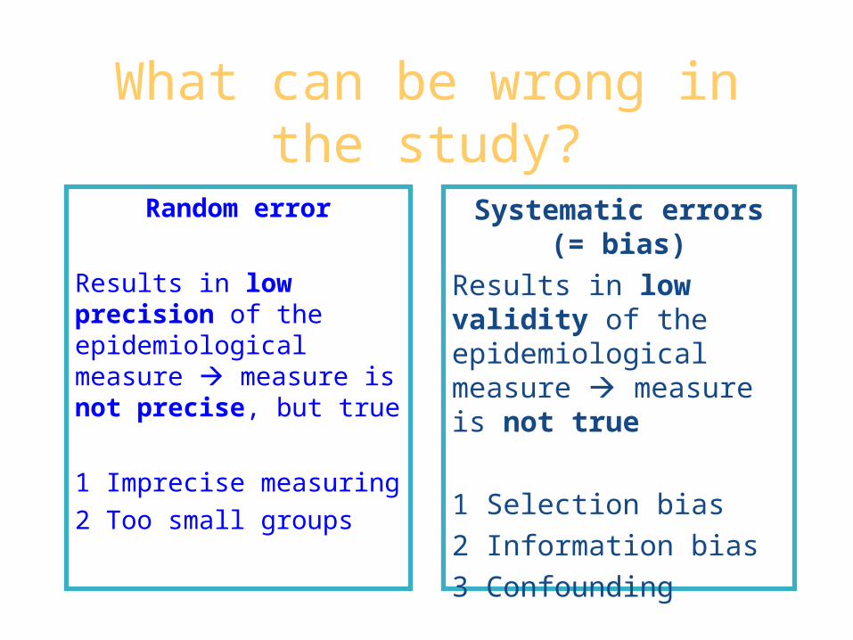
What can be wrong in the study?

Random error

Results in low precision of the epidemiological measure measure is not precise, but true

1 Imprecise measuring

2 Too small groups

Systematic errors(= bias)

Results in low validity of the epidemiological measure measure is not true

1 Selection bias

2 Information bias

3 Confounding

Random errors

Systematic errors

Errors in epidemiological studiesError

Study size

Systematic error (bias)

Random error (chance)

Random error

• Low precision because of– Imprecise measuring– Too small groups

• Decreases with increasing group size

• Can be quantified by confidence interval

Bias in epidemiology1 Concept of bias

2 Classification and controlling of bias

2.1 selective bias

2.2 information bias

2.3 confounding bias

Overestimate?

Underestimate?

Random error ：

Definition

Deviation of results and inferences

from the truth, occurring only as a

result of the operation of chance.

Definition: Systematic, non-random deviation of results and inferences from the truth.

Bias:

2 Classification and controlling of bias

Assembling subjects

collecting data

analyzing data

Selection bias

Information bias

Confounding bias

Time

VALIDITY OF EPIDEMIOLOGIC STUDIES

Reference Population

Study Population

External Validity

Exposed UnexposedInternal Validity

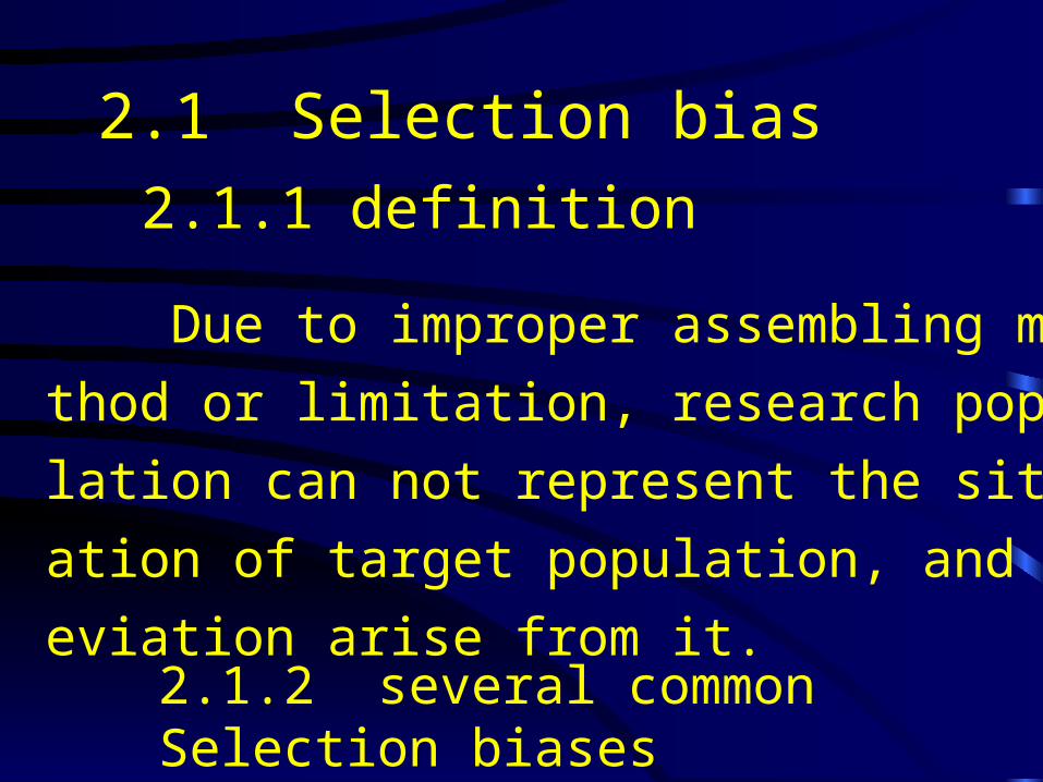
2.1 Selection bias2.1.1 definition

Due to improper assembling method or limitation, research population can not represent the situation of target population, and deviation arise from it.

2.1.2 several common Selection biases

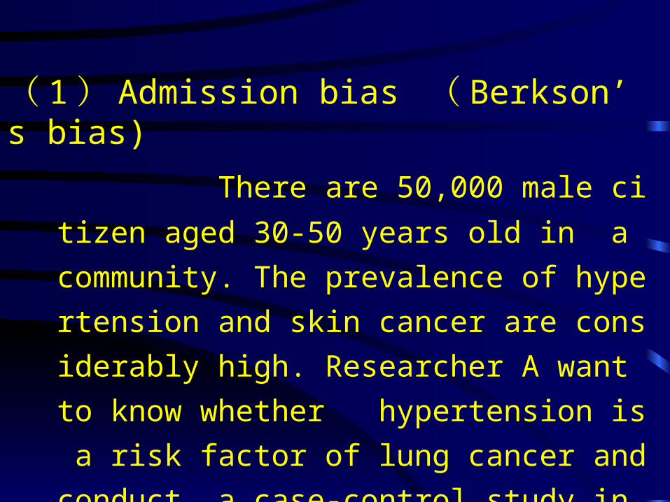
（ 1 ） Admission bias （ Berkson’s bias)

There are 50,000 male citizen aged 30-50 years old in a community. The prevalence of hypertension and skin cancer are considerably high. Researcher A want to know whether hypertension is a risk factor of lung cancer and conduct a case-control study in the community .

case control sum

Hypertension 1000 9000 10000

No hypertension 4000 36000 40000

sum 5000 45000 50000 χ2 =0

OR=(1000×36000)/(9000 ×4000)=1

Researcher B conduct another case-control study in hospital of the community.(chronic gastritis patients as control) .

No association between hypertension and chronic gastritis

admission rate

Lung cancer & hypertension 20%

Lung cancer without hypertension 20%

chronic gastritis & hypertension 20%

chronic gastritis without hypertension 20%

case control sum

hypertension 200 (1000) 200 (2000) 400

No hypertension 800 (4000) 400 (8000) 1200

sum 1000 (5000) 600 (10000) 1600

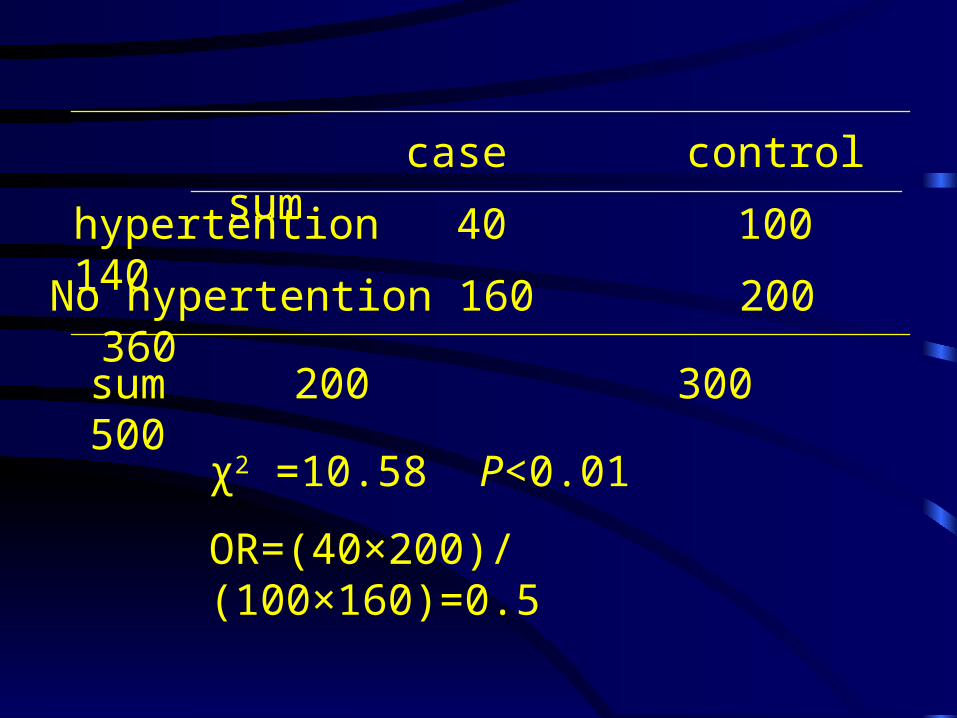
case control sum hypertention 40 100 140

No hypertention 160 200 360

sum 200 300 500

χ2 =10.58 P<0.01

OR=(40×200)/(100×160)=0.5

(2)prevalence-incidence bias （ Neyman’s bias)

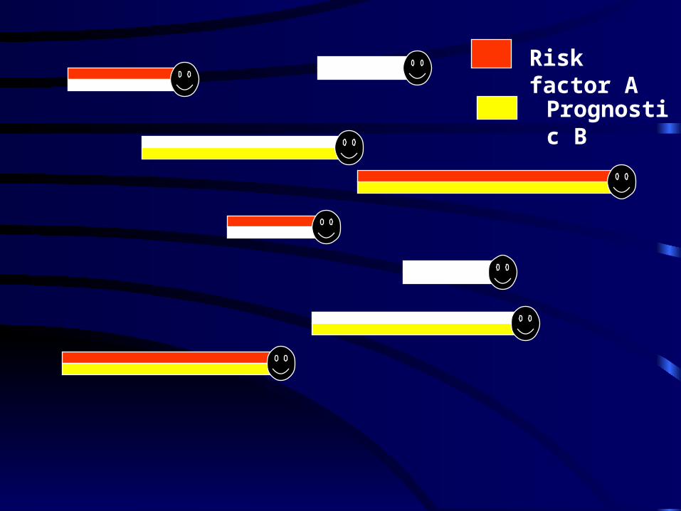
Risk factor A

Prognostic B

A case control sum

exposed 50 25 75

unexposed 50 75 125

sum 100 100 200

χ2 =13.33, P<0.01OR=3

Risk Factor A

Prognostic Factor B

Risk Factor A

Prognostic Factor B

A case control sum

exposed 50 25 75

unexposed 50 75 125

sum 100 100 200

χ2 =13.33, P<0.01OR=3

B case control sum

exposed 80 100 180

unexposed 40 100 140

sum 120 200 320

χ2 =8.47 P<0.01OR=2.0

（ 3 ） non-respondent bias

Survey skills to sensitive question

Abortion

Abortion

yes no

1 2

2 1

Abortion

Yes No

1 2

2 1

number of subjects:N

proportion of red ball:A

numbers who’s answer is “1”:K

Abortion rate: X

Abortion

Yes No

1 2

2 1

number of subjects:N=1000

proportion of red ball:A=40%

numbers who’s answer is “1”:K=540

Abortion rate: X=?

N*A *X+ N*(1-A) *(1-X)=K

（ 4 ） detection signal bias

Endometrium cancer

Intake estrogen

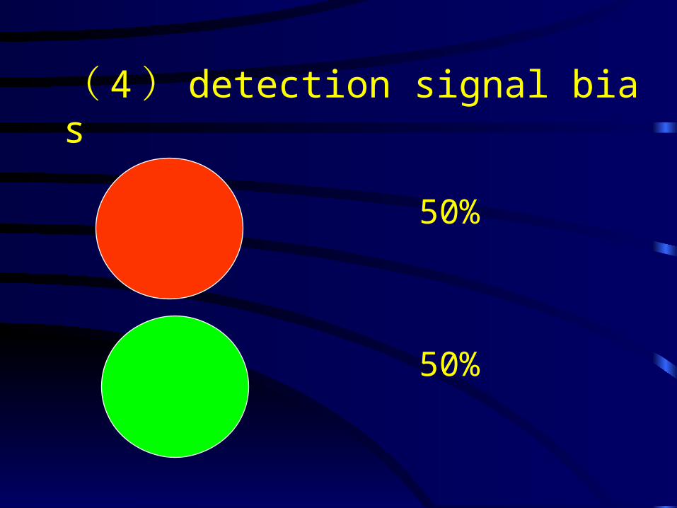
（ 4 ） detection signal bias

50%

50%

Early stage

Terminal stage

Medium stage

50%

Early stage:90%

Medium stage:30%

Terminal stage 5%

Intake estrogen Uterus bleed

Frequently check

Early findout

（ 5 ） susceptibility bias ：

Physical check

drop out

E

UE

2.2 Information Bias

（ 1 ） recalling bias

（ 2 ） report bias

（ 3 ） diagnostic/exposure suspicion bias

(4) Measurement bias

2.3 Confounding bias

Definition:

The apparent effect of the exposure of interest is distorted because the effect of an extraneous factor is mistaken for or mixed with the actual exposure effect.

Properties of a Confounder:

• A confounding factor must be a risk factor for the disease.

• The confounding factor must be associated with the exposure under study in the source population.

• A confounding factor must not be affected by the exposure or the disease.

The confounder cannot be an intermediate step in the causal path between the exposure and the disease.

2.3.2 Control of confounding bias

1 ) restriction

2) randomization

3) matching

1 In designing phase

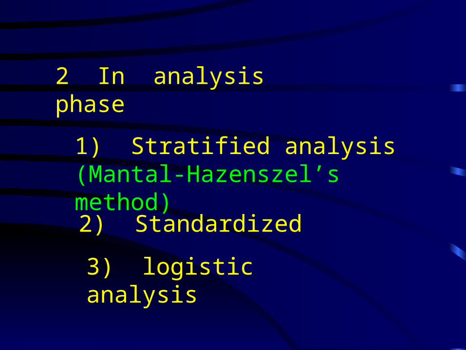
2 In analysis phase

1) Stratified analysis (Mantal-Hazenszel’s method)2) Standardized

3) logistic analysis

A case-control study of Oral contraceptive to myocardial infarction

OC MI control sum + 29 135 164

- 205 1607 1812

sum 234 1742 1976 χ2 =5.84 ,P<0.05 cOR=1.68 OR 95C.I.(1.10,2.56)

Is age a potential confounding factor?

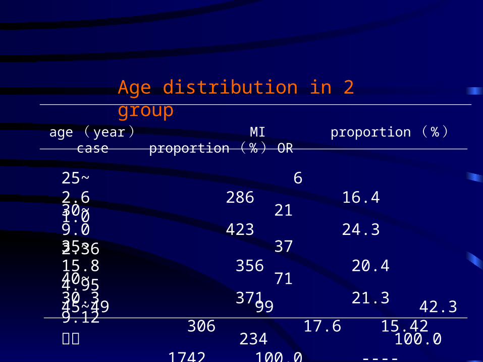
Age distribution in 2 group

age （ year ） MI proportion （ % ） case proportion （ % ） OR

25~ 6 2.6 286 16.4 1.0 30~ 21 9.0 423 24.3 2.36 35~ 37 15.8 356 20.4 4.95 40~ 71 30.3 371 21.3 9.12 45~49 99 42.3 306 17.6 15.42 合计 234 100.0 1742 100.0 ----

OC exposure proportion in different age groups（ % ）

OC exposure in MI Age

（ year ） + - sum

exposure

Proportion(%)

OC exposure in control

+ - sum exposure

Proportion(%)

25~ 4 2 6 66.7 62 224 286 21.7

30~ 9 12 21 42.9 33 390 423 7.8

35~ 4 33 37 10.8 26 330 356 7.3

40~ 6 65 71 8.5 9 362 371 2.4

45~49 6 93 99 6.1 5 301 306 1.6

sum 29 205 234 12.4 135 1607 1742 7.7

χ2 =38.99 P<0.01 χ2 =108.43 P<0.01

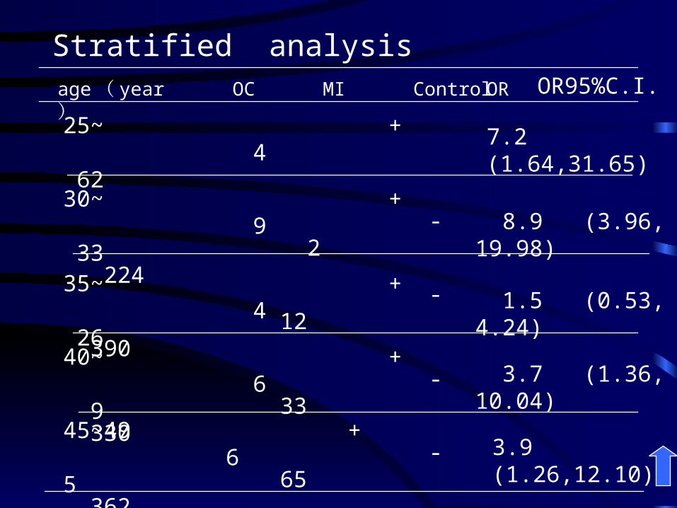
Stratified analysisage （ year ） OC MI Control OR

25~ + 4 62

- 2 224

OR95%C.I.

7.2 (1.64,31.65)

30~ + 9 33

- 12 390 8.9 (3.96,19.98)

35~ + 4 26

- 33 330 1.5 (0.53,4.24)

40~ + 6 9

- 65 362 3.7 (1.36,10.04)

45~49 + 6 5

- 93 3013.9 (1.26,12.10)

Woolf’s Chi-square test

χ2 =6.212

P<0.05,

ν=5-1=4

Incorporate OR

ORMH=3.97

%7.5597.3

97.368.1%100

)(

adjustedOR

adjustedORcrudeOR

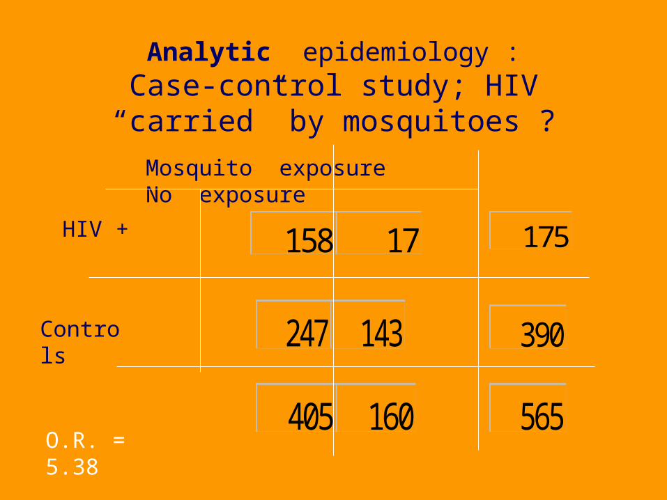
Analytic epidemiology :Case-control study; HIV “carried” by

mosquitoes ?

175HIV +

390Controls

Mosquito exposure No exposure

565

158 17

247 143

405 160O.R. = 5.38

Analytic epidemiology : stratification for confounding ; Case-control study. HIV “carried” by mosquitoes ?

No exposure

Mosquito Exposure

Females HIV + 3 2

166 133

304

Males HIV + 155 15

controls 81 10

261

Mosquito Exposure

O.R. = 1.21

O.R. = 1.27