SANDIA REPORTSAND2006-xxxxUnlimited ReleasePrinted November 2006

Beyond the Local Density Approximation:Improving Density Functional Theory forHigh Energy Density Physics Applications

Normand A. Modine, Alan F. Wright,Richard P. Muller, Mark P. Sears, Ann E. Mattsson,and Michael P. Desjarlais

Prepared bySandia National LaboratoriesAlbuquerque, New Mexico 87185 and Livermore, California 94550

Sandia is a multiprogram laboratory operated by Sandia Corporation,a Lockheed Martin Company, for the United States Department of Energy’sNational Nuclear Security Administration under Contract DE-AC04-94-AL85000.

Approved for public release; further dissemination unlimited.

SAND2006-7540

Issued by Sandia National Laboratories, operated for the United States Department of Energy by Sandia

Corporation.

NOTICE: This report was prepared as an account of work sponsored by an agency of the United States

Government. Neither the United States Government, nor any agency thereof, nor any of their employees,

nor any of their contractors, subcontractors, or their employees, make any warranty, express or implied,

or assume any legal liability or responsibility for the accuracy, completeness, or usefulness of any infor-

mation, apparatus, product, or process disclosed, or represent that its use would not infringe privately

owned rights. Reference herein to any specific commercial product, process, or service by trade name,

trademark, manufacturer, or otherwise, does not necessarily constitute or imply its endorsement, recom-

mendation, or favoring by the United States Government, any agency thereof, or any of their contractors

or subcontractors. The views and opinions expressed herein do not necessarily state or reflect those of

the United States Government, any agency thereof, or any of their contractors.

Printed in the United States of America. This report has been reproduced directly from the best available

copy.

Available to DOE and DOE contractors fromU.S. Department of Energy

Office of Scientific and Technical Information

P.O. Box 62

Oak Ridge, TN 37831

Telephone: (865) 576-8401

Facsimile: (865) 576-5728

E-Mail: reports@adonis.osti.gov

Online ordering: http://www.osti.gov/bridge

Available to the public fromU.S. Department of Commerce

National Technical Information Service

5285 Port Royal Rd

Springfield, VA 22161

Telephone: (800) 553-6847

Facsimile: (703) 605-6900

E-Mail: orders@ntis.fedworld.gov

Online ordering: http://www.ntis.gov/help/ordermethods.asp?loc=7-4-0#online

DEP

ARTMENT OF ENERGY

• • UN

ITED

STATES OF AM

ERI C

A

2

SAND2006-xxxxUnlimited Release

Printed November 2006

Beyond the Local Density Approximation: ImprovingDensity Functional Theory for High Energy Density

Physics Applications

Normand A. Modine and Alan F. WrightPhysical, Chemical, & Nano Sciences Center

Richard P. Muller, Mark P. Sears, and Ann E. MattssonComputation, Computers, Information and Mathematics Center

Michael P. DesjarlaisPulsed Power Sciences Center

Sandia National LaboratoriesP.O. Box 5800

Albuquerque, NM 87185

Abstract

A finite temperature version of ”exact-exchange” density functional theory (EXX) has been im-plemented in Sandia’s Socorro code. The method uses the optimized effective potential (OEP)formalism and an efficient gradient-based iterative minimization of the energy. The derivation ofthe gradient is based on the density matrix, simplifying the extension to finite temperatures. Astand-alone all-electron exact-exchange capability has been developed for testing exact exchangeand compatible correlation functionals on small systems. Calculations of eigenvalues for the he-lium atom, beryllium atom, and the hydrogen molecule are reported, showing excellent agreementwith highly converged quantum Monte Carlo calculations. Several approaches to the generation ofpseudopotentials for use in EXX calculations have been examined and are discussed. The difficultproblem of finding a correlation functional compatible with EXX has been studied and some initialfindings are reported.

3

Acknowledgments

We are indebted to Ross Lippert of MIT for his substantial contributions to this work, particularlywith regard to the mathematical developments discussed in Chapter 2 and published in Ref. [16].This work would not have been possible without the combined support of the High Energy DensityPhysics (HEDP) and Materials Science and Technology (MS&T) LDRD Investment Areas. Wewould also like to thank Charles Barbour, John Aidun, and Tom Mehlhorn for their early andcontinued support of this project.

4

Contents

Nomenclature . . . . . . . . . . . . . . . . . . . . . . . . . . . . . . . . . . . . . . . . . . . . . . . . . . . . . . . . . . . 10

1 Introduction and Motivation 11

2 Mathematics of the optimized effective potential (OEP) 13

Introduction . . . . . . . . . . . . . . . . . . . . . . . . . . . . . . . . . . . . . . . . . . . . . . . . . . . . . . . . . . . . . 13

The perturbation theory of matrix-analytic functions . . . . . . . . . . . . . . . . . . . . . . . . . . . . . 14

Practical application of the Jacobian . . . . . . . . . . . . . . . . . . . . . . . . . . . . . . . . . . . . . 16

Density functional theory review . . . . . . . . . . . . . . . . . . . . . . . . . . . . . . . . . . . . . . . . . . . . 18

Finite temperature OEP with density operators . . . . . . . . . . . . . . . . . . . . . . . . . . . . . . . . . 18

Finite temperature OEP with orbitals . . . . . . . . . . . . . . . . . . . . . . . . . . . . . . . . . . . . . . . . . 21

Computational results . . . . . . . . . . . . . . . . . . . . . . . . . . . . . . . . . . . . . . . . . . . . . . . . . . . . . 22

Finite Basis Set Issues . . . . . . . . . . . . . . . . . . . . . . . . . . . . . . . . . . . . . . . . . . . . . . . . . . . . . 26

A truly degenerate case . . . . . . . . . . . . . . . . . . . . . . . . . . . . . . . . . . . . . . . . . . . . . . . 27

The origin of the pathology . . . . . . . . . . . . . . . . . . . . . . . . . . . . . . . . . . . . . . . . . . . . 28

Plane-wave calculations . . . . . . . . . . . . . . . . . . . . . . . . . . . . . . . . . . . . . . . . . . . . . . . 28

Discussion . . . . . . . . . . . . . . . . . . . . . . . . . . . . . . . . . . . . . . . . . . . . . . . . . . . . . . . . . . . . . . 29

3 Implementation of the OEP in Socorro 31

Review of the OEP . . . . . . . . . . . . . . . . . . . . . . . . . . . . . . . . . . . . . . . . . . . . . . . . . . . . . . . 31

Review of the application of∆ω∆ε [·] . . . . . . . . . . . . . . . . . . . . . . . . . . . . . . . . . . . . . . . . . . . 33

Iterative Algorithms . . . . . . . . . . . . . . . . . . . . . . . . . . . . . . . . . . . . . . . . . . . . . . . . . . . . . . 34

Preconditioning the Outer Loop . . . . . . . . . . . . . . . . . . . . . . . . . . . . . . . . . . . . . . . . . . . . . 35

5

Potential cut-offs . . . . . . . . . . . . . . . . . . . . . . . . . . . . . . . . . . .. . . . . . . . . . . . . . . . . . . . . . 39

OEP Hellman-Feynman correction . . . . . . . . . . . . . . . . . . . . . . . . . . . . . . . . . . . . . . . . . . . 40

4 Tests and Applications 43

Convergence Tests . . . . . . . . . . . . . . . . . . . . . . . . . . . . . . . . . . . . . . . . . . . . . . . . . . . . . . . . 43

EXX results for H2 and bulk Si and Ge . . . . . . . . . . . . . . . . . . . . . . . . . . . . . . . . . . . . . . . 46

EXX results for the silicon interstitial . . . . . . . . . . . . . . . . . . . . . . . . . . . . . . . . . . . . . . . . . 47

5 Pseudopotentials 49

6 Small system tests of the OEP 51

Helium Atom. . . . . . . . . . . . . . . . . . . . . . . . . . . . . . . . . . . . . . . . . . . . . . . . . . . . . . . . . . . . 51

Beryllium Atom . . . . . . . . . . . . . . . . . . . . . . . . . . . . . . . . . . . . . . . . . . . . . . . . . . . . . . . . . 51

Hydrogen Molecule . . . . . . . . . . . . . . . . . . . . . . . . . . . . . . . . . . . . . . . . . . . . . . . . . . . . . . . 53

Finite Temperature EXX Simulations . . . . . . . . . . . . . . . . . . . . . . . . . . . . . . . . . . . . . . . . . 54

7 Correlation compatible with Exact Exchange 55

Appendix

A Expressions for the Exchange Energy and Exchange Derivative 61

References . . . . . . . . . . . . . . . . . . . . . . . . . . . . . . . . . . . . . . . . . . . . . . . . . . . . . . . . . . . . . . 69

6

List of Figures

2.1 A comparison of the energy change predicted from the gradient and the actualenergy change observed during a random walk in the potential. The filled circlesare the calculated values. The solid line is a guide to the eye representing perfectagreement. . . . . . . . . . . . . . . . . . . . . . . . . . . . . . . . . . . . . . . . . . . . . . . . . . . . . . . . . . 24

2.2 The error in the energy, as well as the square-norm of gradient, during the iterativeminimization on a log scale. . . . . . . . . . . . . . . . . . . . . . . . . . . . . . . . . . . . . . . . . . . . 25

4.1 A comparison of the energy change predicted from the gradient and the actualenergy change observed during a random walk in the potential. The crosses are thecalculated values. The solid line is a guide to the eye representing perfect agreement. 44

4.2 The convergence of theexact exchangeenergy, as well as the square-norm ofgradient, during the iterative minimization on a log scale. The top plot was runat room temperature (25.67 meV) and the bottom at high temperature (1 eV).g =

∂E∂V(r) from (2.25). . . . . . . . . . . . . . . . . . . . . . . . . . . . . . . . . . . . . . . . . . . . . . . . . . . . 45

4.3 Our calculated band gap of silicon as a function of temperature using EXX and theLDA. . . . . . . . . . . . . . . . . . . . . . . . . . . . . . . . . . . . . . . . . . . . . . . . . . . . . . . . . . . . . . 47

4.4 The Kohn-Sham eigenvalues obtained from a 217 atom calculation for the -2 chargestate of the silicon self-interstitial using EXX and the PBE. The eigenvalues aregiven relative to the valence band edge. . . . . . . . . . . . . . . . . . . . . . . . . . . . . . . . . . . 48

5.1 A comparison of Si pseudopotentials computed (top) using the Fritz-Haber pseu-dopotential code with the LDA XC functional, (center) using the Fritz-Haber pseu-dopotentialcode with the KLI XC functional, (bottom) using the Engels group’spseudopotential code with the EXX XC functional. . . . . . . . . . . . . . . . . . . . . . . . . . 50

6.1 A comparison of the excitation energies for different states of Helium atom, us-ing the Hartree-Fock (HF) method, and density functional theory using the LDA,BLYP, PBE, B3LYP functionals, as well as the EXX and EXX-GVB method de-velop in this LDRD project. . . . . . . . . . . . . . . . . . . . . . . . . . . . . . . . . . . . . . . . . . . . . 52

7

6.2 A comparison of the excitation energies for different states of Beryllium atom,using the Hartree-Fock (HF) method, and density functional theory using the LDA,BLYP, PBE, B3LYP functionals, as well as the EXX method develop in this LDRDproject. . . . . . . . . . . . . . . . . . . . . . . . . . . . . . . . . . . . . . . . . . . . . . . . . . . . . . . . . . . . . 52

6.3 A comparison of the dissociation behavior of different density functionals showingthat traditional gradient-corrected density functionals (BLYP), hybrid functionals(B3LYP), and even simple OEP/EXX functionals produce energies that are incor-rect for molecular hydrogen at geometries with stretched H–H bonds. In contrast, amethod from the current work (EXX/GVB) does in fact produces correct energiesfor the stretched hydrogen geometries. . . . . . . . . . . . . . . . . . . . . . . . . . . . . . . . . . . . 53

6.4 A comparison of the band gaps versus temperature using the Hartree-Fock (blue),LDA (green) and EXX (red) methods. Note that the band gap of the EXX methodapproaches the LDA method at sufficiently high temperatures. . . . . . . . . . . . . . . . . 54

7.1 Examples of two jellium surface densities with differentrs-values.rs = 2.07 cor-responds to the valence electron density in aluminum. Largerrs corresponds tolower density. . . . . . . . . . . . . . . . . . . . . . . . . . . . . . . . . . . . . . . . . . . . . . . . . . . . . . . . 55

7.2 Examples of two possible indices to interpolate between ’interior’ (LDA correla-tion, index=1) and edge region (index=0) . . . . . . . . . . . . . . . . . . . . . . . . . . . . . . . . . 58

7.3 Accumulated surface correlation energy. . . . . . . . . . . . . . . . . . . . . . . . . . . . . . . . . . . 60

8

List of Tables

7.1 Exchange surface energies, in erg/cm2, for the jellium surface model. Mean abso-lute relative errors (mare) are compared to the EXX results [28]. . . . . . . . . . . . . . . . 56

7.2 Correlation surface energies, in erg/cm2, for the jellium surface model. Meanabsolute relative errors (mare) are compared to the RPA+ results [29]. . . . . . . . . . . 57

7.3 Exchange-correlation surface energies, in erg/cm2, for the jellium surface model.Mean absolute relative errors (mare) are compared to the EXX/RPA+ results. . . . . . 57

9

Nomenclature

HEDS High Energy Density Science

DFT Density Functional Theory

OEP Optimized Effective Potential

EXX Exact Exchange

HF Hartree-Fock

LDA Local Density Approximation

PZ A parametrisation of the Ceperley-Alder [35] LDA correlation created by Perdew and Zunger [32]

PW A parametrisation of the Ceperley-Alder [35] LDA correlation created by Perdew and Wang [31]

GGA Generalized Gradient Approximation

PBE A GGA created by Perdew, Burke, and Ernzerhof [33]

PW91 A GGA created by Perdew et al. [34]

RPA+ An enhanced Random Phase Approximation [29]

h Planck’s constant= 1.05459×10−34 J ·s

me Electron mass= 9.1095×10−31 kg

e Electron charge= 1.60219×10−19 As

ε0 Vacuum permittivity= 8.85419×10−12 As/Vm

a0 Bohr radius= h2/(me(e2/(4πε0))) = 0.529177×10−10 m

n Density

10

Chapter 1

Introduction and Motivation

An integral component of the High Energy Density Science (HEDS) work done at Sandia is theuse of advanced modeling codes such as ALEGRA to simulate the complex evolution of materi-als through solid, liquid, vapor, and plasma phases in HEDS experiments. These codes requireaccurate equation-of-state (EOS), conductivity, and opacity models if high-fidelity results are tobe obtained. A particularly difficult region to characterize is the “warm dense matter” regimethat extends from near solid conditions into the vapor dome and temperatures up to several eV.This region of phase space includes the molecular-to-atomic dissociation phase for dense hydro-gen and its isotopes, and the metal-insulator transition for liquid metals. In recent years, muchprogress has been made in the understanding and accurate modeling of these regimes through theuse of quantum molecular dynamics based on finite temperature density-functional theory (FT-DFT), which enables the calculation of manifestly consistent EOS, conductivities, and low-energyopacities [1, 2, 3, 4]. Although the application of density functional methods to high energy den-sity science is rather new, DFT is a powerful and commonly used tool in Material Science andTechnology (MS&T) research. Applications include surface science, the properties of water, thestudy of defects in materials, insulators, complex materials, optical ceramics, and oxides.

The commonly used DFT codes of today employ relatively simple but efficient, explicit function-als of the density, categorized as local density or generalized gradient approximations (LDA andGGA), respectively. These functionals have proven to give quite accurate results for many prop-erties of interest. However, as numerical methods have evolved, and large systems and complexproblems have been studied with high precision, the deficiencies of these functionals have becomethe limiting factor to needed improvements in accuracy. It is well-known that LDA and GGAfunctionals typically underestimate the energy gap between occupied (valence) and unoccupied(conduction) bands by 1 to 2 eV, shifting behavior more towards a metal and underestimating met-allization densities and pressures. In HEDS applications, when the temperature is comparable to orsmaller than the gap, the conductivity and the low-energy opacities will be significantly increased.In these HEDS applications it is often the case that the temperature is high enough to thermallypopulate many of the conduction bands, and therefore corrections to the band gap have a corre-sponding effect on the pressure and energy, as well as the conductivity and optical properties. Theonly way to self-consistently improve calculations where the erroneous gap influences the resultsis to develop and use an improved functional. Improvements to the accuracy of the exchange func-tional will provide a significantly enhanced tool for MS&T research as well. For example, sincedefect formation energies and charges depend on the position of defect levels in the gap, improve-

11

ment in band gaps will help in identifying defects and predicting defect populations, kinetics, andproperties during growth and processing, and following radiation damage in materials of interestto Sandia (e.g., alumina).

Accordingly, we have developed and implemented a much more advanced treatment of the exchange-correlation functional into Sandia’s state-of-the art plane-wave DFT computational framework, So-corro. This approach centers on using the known exact expression for exchange in the functional.The exact expression is a highly non-local, implicit functional of the density (an explicit functionalof the Kohn-Sham orbitals). Doing this leaves the evaluation of the smaller correlation contributionas the only remaining approximation. Several groups have already performed small-scale investi-gations of this sort. Use of exact exchange (EXX) is found to essentially solve the band gap andmetallization problems. It remains an important and challenging problem to combine EXX-DFTwith molecular dynamics for systems of several tens to hundreds of atoms, but the potential returnis broadly important and should have enduring impact in computational material science.

12

Chapter 2

Mathematics of the optimized effectivepotential (OEP)

Introduction

The Kohn-Sham Density Functional Theory (DFT) [5] has become one of the most powerful toolsfor understanding and predicting the properties of materials. DFT has been applied to an everincreasing number of different types of systems and phenomena, and the results have frequentlybeen remarkably useful. Nevertheless, the accuracy of the results remains an important issue formany potential applications of DFT. The main source of error in DFT calculations is the use ofan approximate expression for the exchange-correlation energy,EXC. Such an approximation isnecessary for practical calculations, but improving the quality of the approximation, and hence,the accuracy of the calculations, is of great interest. Conventional variants of DFT, such as LDAand GGA, takeEXC to be an explicit functional of the electronic density. Since the noninter-acting Kohn-Sham orbitals are implicit functionals of the electronic density [6], expressions forEXC that explicitly depend on the Kohn-Sham orbitals are also consistent with the DFT frame-work. An important example of such a functional is the functional used in the exact-exchangeapproximation[7, 8, 9, 10, 11, 12, 13]. An explicit dependence on the orbitals allows approximateEXC expressions to capture physical behaviors of the exact Kohn-ShamEXC that can not be practi-cally incorporated in an expression that is an explicit function of only the electronic density. Oneexample is the absence of self-interaction in the exact Kohn-Sham energy. Another example is thecomplex, non-local behavior of the exact exchange energy.

The difficulty in using anEXC expression that is explicitly dependent on the orbitals is that it isimpossible to straightforwardly take the functional derivative ofEXC with respect to the electronicdensity. Therefore, standard self-consistent methods of minimizing the energy with respect to thedensity can not be used. The solution to this problem is provided by the Optimized EffectivePotential (OEP) formalism. Since the energy is a functional of the Kohn-Sham orbitals, and theorbitals are solutions of the Kohn-Sham equation for some local potential, the energy can be viewedas a functional of the potential. The OEP is defined to be the potential that minimizes the energy.This minimization with respect to the potential is equivalent to the usual minimization with respectto the density. Traditionally, the OEP has been calculated by solving the OEP integral equation,in which the gradient of the energy with respect to the potential is set to zero [7, 8, 9, 11], or by

13

directly evaluating and inverting a response function [10, 12, 13].

Two recent papers have proposed calculation of the OEP by means of an iterative minimization ofthe energy [14, 15]. Hyman, Stiles, and Zangwill used Lagrange multiplier methods to derive anexpression for the gradient of the energy with respect to the potential and proposed using this gra-dient to minimize the energy iteratively. Kummel and Perdew derived a nearly identical expressionand, although they did not claim that this expression gives the gradient, they noted that it providesa good update to the potential during an iterative minimization. In this paper, we present a newderivation of the gradient based on the density matrix. Our work goes beyond the previous papersin the following ways: (1) We believe that our derivation is particularly transparent, and therefore,it demonstrates that this expression is, in fact, the correct gradient. (2) The previous work assumeda negligible electronic temperature. Since our derivation is based on the density matrix, it is easilyextended to finite temperatures, where the orbitals are partially occupied.

One of the most exciting recent applications of DFT has been high energy density physics. Inthis application, electronic temperatures that are substantial compared to the band gaps of typicalsemiconductors are common. This makes the results sensitive to the band gap, which is too small inthe standard versions of DFT. Therefore, the capability of performing calculations with advancedfunctionals that have explicit dependence on the orbitals at non-zero temperature is particularlyexciting for high energy density physics applications.

As an alternative to iterative minimization of the energy using the gradient, it is possible, in prin-ciple, to find the OEP by solving the equation in which the gradient is set to zero. Therefore, ourwork provides the finite temperature equivalent of the standard OEP equation, giving the correctnecessary condition for local optimality.

In this article, we derive the OEP method in a finite temperature regime by considering the pertur-bation of the density matrix resulting from a perturbed Hamiltonian. The gradient will reduce to acombination of orbital shifts as one sees in the zero temperature limit plus some corrections whichcome from the finite temperature. In section 2, we begin with a mathematical discussion of theperturbation theory of analytic functions of Hermitian operators. After a short review of densityfunctional theory, we apply the results of Section 2 to the density matrixρ viewed as a function ofthe Kohn-Sham HamiltonianH, and thereby derive a finite temperature OEP equation in terms ofH andρ . This motivates the subsequent section, which describes the gradient expression inorbitalform. We conclude with some computational results demonstrating the accuracy of the method. Amore streamlined version of these results with alternative derivations of some of the expressionshas been published recently [16].

The perturbation theory of matrix-analytic functions

Let f (x) be an analytic function ofx and f (A) be the extension off to a matrix-analytic function(see [17], chapter 6) on some algebra of Hermitian operators with a finite (or countable) spectrum.

14

Thus,

[A, f (A)] = A f(A)− f (A)A = 0 (2.1)

fi = f (ai) (2.2)

where theai are the eigenvalues ofA and thefi are the eigenvalues off (A).

For an unconstrained variationA→ A+δA the variations of (2.1) and (2.2) are

[δA, f (A)]+ [A,δ f (A)] = 0 (2.3)

δ fi = f ′(ai)δai . (2.4)

In a basis whereA is diagonal (ai = Aii , f (ai) = [ f (A)]ii ), (2.3) and (2.4) become,

(ai−a j) [δ f (A)]i j = ( f (ai)− f (a j))δAi j (2.5)

δ [ f (A)]ii = f ′(ai)δAii . (2.6)

Thus (2.3) and (2.4) appear to be sufficient to determineδ f (A) in terms ofA,δA.

We may, somewhat informally, write the result as one equation

[δ f (A)]i j =f (ai)− f (a j)

ai−a jδAi j (2.7)

where it is understood that we treatf (ai)− f (a j )ai−a j

as adivided difference, taking the limit asai → a j .

A more rigorous proof of these results can be made in the following theorem, which also makesclear what happens in the presence of a repeated eigenvalue.

Theorem 2.0.1 The expansion of f(A+δA)− f (A) = δ f (A) to first order inδA is given by

[δ f (A)]i j = limε→0

f (ai + ε)− f (a j)

ai−a j + εδAi j

where the matrix elements are taken in an basis in which A is diagonal.

Proof: Since f is analytic, it suffices to prove this theorem forf (x) = xk and extend by linearity.

δ f (x) = ∑m+n=k−1

AmδAAn

15

in a diagonal basis,

[δ f (x)]i j = ∑m+n=k−1

ami an

j δAi j

= ∑m+n=k−1

limε→0

(ai + ε)manj δAi j

= limε→0

(ai + ε)k−akj

(ai + ε)−a jδAi j

and the summation is interchanged with the limit.

Note that one could clearly obtain higher order derivatives in terms of higher order divided differ-ences via the same approach. To simplify forthcoming derivations, we omitε ’s and limits, with theunderstanding that appropriate limits are to be taken for divided differences of the formf (x)− f (y)

x−y .

We may interpret (2.7) as the equation which specifies the action of theJacobian, ∂ f (A)∂A on an

arbitrary Hermitian operator of the mappingf .

Practical application of the Jacobian

An A-diagonalizing basis might not be a convenient means to compute the application of the Jaco-bian to an arbitrary variation. We present here a short digression on how such computations can becarried out iteratively, without diagonalizingA.

We will be interested in applications of linear operators to Hermitian (or anti-Hermitian) matrices.To avoid some of the confusion entailed inoperators of operatorsdiscussions, we introduce somenotation, which we hope is clarifying. We denote the application of a linear operator on a matrixwith brackets,L [A]. In terms of indices we may write this asL [A]i j = ∑kl Li jkl Akl. For Hermitianmatrices, we write〈X,Y〉= trXY, and it is well known that this is a non-degenerate inner producton the vector space of Hermitian matrices. For a vector subspace of Hermitian matrices,A, we letA⊥ = B : ∀X ∈ A,〈X,B〉= 0.

We denote the linear action of a commutator adX [Y] =−adY [X] = [X,Y].

Lemma 2.0.2

〈X,adY[Z]〉=−〈adY[X],Z〉 .

Proof: Applying the trace identity trAB= trBA,

trX(YZ−ZY) = trXYZ−YXZ= −tr(YX−XY)Z

16

Thecentralizerof X is the setCX = Y : [X,Y] = 0. CX is the nullspace of adX.

Lemma 2.0.3 C⊥X is the range of adX.

Proof: For anyY and someZ ∈ CX, by lemma 2.0.2,〈adX(Y),Z〉 = −〈Y,adX(Z)〉 = 0, thusRangeadX ⊂C⊥X .

From elementary dimension counting,

dimRangeadX+dimNulladX = dimCX+dimC⊥X dimRangeadX+dimCX = dimCX+dimC⊥X

dimRangeadX = dimC⊥X

where dimCX= dimCX obtains the last line.

Let Xi j =f (ai)− f (a j )

ai−a jYi j in anA-diagonalizing basis. Then according to (2.1) and (2.3),

adA[X] = adf (A)[Y]. (2.8)

The operator, adA, has a non-trivial nullspace. However,CA ⊂ Cf (A) implies Rangeadf (A) ⊂RangeadA, by lemma 2.0.3, thus equation (2.8) has a unique solution.

Since we are dealing with a linear space (albeit of matrices), with a linear operator and an innerproduct, we can use a Krylov-based iterative solver to solve (2.8) (e.g. conjugate gradient orMINRES [18, 19]) with some initial guess,X0, yielding

X = X0+c1adA[X0]+c2ad2A[X0]+ · · ·

with X−X0 ∈C⊥A .

By (2.4), we additionally requireXii = f ′(ai)Yii . For example, if we take

X0 =12

(

f ′(A)Y+Y f ′(A))

+X1,

whereX1 ∈C⊥A is arbitrary, then the iterative solution of (2.8) will be correct, i.e.X = δ f (A). Inthe remainder of this article we takeX1 = 0.

17

Density functional theory review

Let ρ be a density matrix (Hermitian),K be the kinetic energy operator,VI be the ionic (andexternal) potential, withEHXC(ρ) the Hartree, exchange, and correlation energy. WithS(P) =−trρ log(ρ)+(I −ρ) log(I −ρ) as the entropy expression, the variational energy is

E(ρ) = trρ(K +VI )+EHXC(ρ)− 1β

S(ρ). (2.9)

The unconstrained derivative is

∂E∂ρ

= K +VI +∂EHXC

∂ρ+

1β

log(ρ(I −ρ)−1). (2.10)

The Kohn-Sham Hamiltonian is given byH = K +VI +V whereV is the self-consistent potential(to be determined). In the Kohn-Sham DFT,ρ is the minimizer of trρH− 1

β S(ρ) with trρ= n,which is equivalent to the conditions,

ρ =1

1+eβ (H−µI)= fβ (H−µI) (2.11)

trρ = n (2.12)

for some chemical potentialµ. Thus, we can considerρ to be parametrized by two unknownsV and µ with two relations (2.11) and (2.12). Note: one could absorbµ into V, but we find itadvantageous to keep it distinct in its role as a Lagrange multiplier.

With ρ satisfying these relations, the energy differential simplifies

∂E∂ρ

= K +VI +∂EHXC

∂ρ+

1β

log(ρ(I −ρ)−1)

= K +VI +∂EHXC

∂ρ− (H−µI)

=∂EHXC

∂ρ− (V−µI).

Finite temperature OEP with density operators

From section 2, the density matrix is related to the Kohn-Sham Hamiltonian,H, by (2.11) and(2.12). Letεi be the eigenvalues ofH, and letωi = fβ (εi−µ) be the eigenvalues ofρ . The divided

18

differences can be stably computed with the formula

fβ (x)− fβ (y)

x−y=− eβ (x+y)/2

(1+eβx)(1+eβy)

(

sinh(β (x−y)/2)

(x−y)/2

)

where a test forx = y is required for the evaluation of the last factor. We note in particular thatfβ (x)− fβ (x)

x−x = ddx fβ (x) =−β fβ (x)(1− fβ (x)).

Let E(ρ) be a function of a density matrix,ρ . We can implicitly defineE(H) = E(ρ(H,µ(H))).Formally varyingE(H),

δE(H) = tr

∂E(ρ(H,µ))

∂ρδρ

. (2.13)

in anH-diagonalizing basis,

δρi j =ωi −ω j

εi− ε j

(

δHi j −δ µδi j)

. (2.14)

By (2.12), the trace ofδρ vanishes,

δ µ =∑i j δi j

ωi−ω jεi−ε j

δHi j

∑i j δi jωi−ω jεi−ε j

=trρ(I −ρ)δH

trρ(I −ρ) .

Thus, in anH-diagonalizing basis,

δE = ∑i j

∂E∂ρi j

ωi−ω j

εi− ε j

(

δHi j −δ µδi j)

= ∑i j

∂E∂ρi j

ωi−ω j

εi− ε j

(

δHi j −∑k ωk(1−ωk)δHkk

∑k ωk(1−ωk)δi j

)

= ∑i j

(

ωi−ω j

εi− ε j

∂E∂ρi j−δi j

ωi(1−ωi)

∑k ωk(1−ωk)∑pq

δpqωp−ωq

εp− εq

∂E∂ρpq

)

δHi j

19

and the gradient is therefore

∂E∂Hi j

=ωi−ω j

εi− ε j

∂E∂ρi j−δi j

ωi(1−ωi)

∑k ωk(1−ωk)∑pq

δpqωp−ωq

εp− εq

∂E∂ρpq

(2.15)

∂E∂H

=∆ω∆ε

[

∂E∂ρ

]

− ρ(I −ρ)

trρ(I −ρ) tr

∆ω∆ε

[

∂E∂ρ

]

(2.16)

=∆ω∆ε

∂E∂ρ−

tr

∆ω∆ε

[

∂E∂ρ

]

tr∆ω

∆ε [I ] I

(2.17)

where ∆ω∆ε [·] stands for the Jacobian,ωi−ω j

εi−ε j, in a general basis. tr

∆ω∆ε [I ]

= −β trρ(I − ρ),though we will keep it as it is in (2.17) to make the tracelessness of∂E

∂H more manifest.

The application of the Jacobian, to obtain∂E∂H = ∆ω

∆ε

[

∂E∂ρ −

tr

∆ω∆ε

[

∂E∂ρ

]

tr∆ω∆ε [I ] I

]

, can be done by iteratively

solving

[

H,∂E∂H

]

=

[

ρ,∂E∂ρ

]

(2.18)

with initial guess

(

∂E∂H

)

0= −1

2β(

ρ(I −ρ)∂E∂ρ

+∂E∂ρ

ρ(I −ρ)

)

+βtr

∆ω∆ε

[

∂E∂ρ

]

tr∆ω

∆ε [I ] ρ(I −ρ). (2.19)

Note: limβ→∞ βρ(I − ρ) ∝ δ (H − µI), a delta function on the spectrum ofH. Thus in the low

temperature limit, only the eigenvalues ofH nearµ contribute to(

∂E∂H

)

0.

To obtain an OEP gradient, we restrict the variability ofH to H = H0 +V whereH0 = K +VI isfixed andV is a local operator. The gradient is then

∂E∂V(r)

= ∑i j

φi(r)∂E

∂Hi jφ∗j (r) (2.20)

whereφi(r) is the eigenvector ofH with eigenvalueεi in the position representation.

20

Finite temperature OEP with orbitals

Instead of representing the density as an operator, it is often more practical to expressρ in termsof an incomplete basis of partially occupied orbitals. Letφ1,φ2, . . . be a complete eigenbasis ofHsorted non-decreasingly in eigenvalue. LetN be sufficiently large thatωi>N ∼ 0. Then we maywrite truncate the basis so that

ρ = φΩφ† (2.21)

whereφ =[

φ1 φ2 · · · φN]

, with Λ the diagonal matrix of eigenvalues andΩ the diagonal matrixwith entriesω1, . . . ,ωN (i.e. Ω = fβ (Λ− µI)). Note, N will usually be much smaller than thenumber of primitive basis functions, soφ will be a rectangular matrix with orthonormal columns,i.e. φ†φ = I (theN×N identity) andφφ† is the orthogonal projector onto the span of theφi (andhence commutes withH).

Let χ andζ be given by

χ = tr

∆ω∆ε

[

∂E∂ρ

]

= ∑i≥1−βωi(1−ωi)φ†

i∂E∂ρ

φi

ζ = tr

∆ω∆ε

[I ]

= ∑i≥1−βωi(1−ωi)

and letE andJ beN×N matrices given by

E = φ†∂E(φΩφ†)

∂ρφ

(

i.e. Ei j =∂E(φΩφ†)

∂ρi j

)

(2.22)

J = φ†∆ω∆ε

[

∂E∂ρ− χ

ζI

]

φ(

i.e. Ji j =ωi−ω j

εi− ε j

(

Ei j −χζ

δi j

))

. (2.23)

Note that by these definitions,[Ω, E] = [Λ, J].

Sinceωi>N ∼ 0, the expressions forχ andζ can likewise be truncated,

χ = ∑1≤i≤N

−βωi(1−ωi)Eii =−β trΩ(I −Ω)E

ζ = ∑1≤i≤N

−βωi(1−ωi) =−β trΩ(I −Ω)

and by (2.15)

(I −φφ†)∆ω∆ε

[

∂E∂ρ− χ

ζI

]

(I −φφ†) = 0,

21

thus, we may write (2.16) as

∂E∂H

=∆ω∆ε

[

∂E∂ρ− χ

ζI

]

= φψ† +ψφ†, (2.24)

whereφ†ψ = ψ†φ = 12J. This gives an orbital form of equation (2.20),

∂E∂V(r)

= ∑1≤i≤N

φi(r)ψ∗i (r)+ψi(r)φ∗i (r) (2.25)

which is similar to the equation derived in numerous sources in the OEP literature [14, 15], with amodification of theψ to accommodate the finite temperature regime.

It remains to solve forψ, which we may decompose asψ = ψ⊥+ 12φ J, whereφ†ψ⊥ = 0. We

can derive an equation forψ⊥, by multiplying equation (2.18) on the left by the projectorI −φφ†

(which commutes withH) and on the right byφ and employing (2.24),

(I −φφ†)

[

H,∂E∂H

]

φ = (I −φφ†)

[

ρ,∂E∂ρ

]

φ (2.26)

(I −φφ†)(Hψ−ψΛ) = −(I −φφ†)∂E∂ρ

ρφ (2.27)

Hψ⊥−ψ⊥Λ = −(I −φφ†)∂E∂ρ

φΩ. (2.28)

The LHS and RHS of (2.28) are orthogonal toφ , by construction. Thus we have a well-definedequation forψ⊥. An iterative method can thus be used to solve forψ⊥ without any special initial-ization beyondφ†ψ⊥ = 0.

Computational results

In order to test the above approach, it was implemented in the orbital representation within theSocorro electronic structure software using a plane wave basis set and norm-conserving pseudopo-tentials. The conjugate gradient algorithm was used to solve the linear systems involved in theevaluation of the gradient. Using this algorithm, the computational cost of solving the set of linearsystems determiningψ⊥ is comparable to the cost of solving the Kohn-Sham eigenproblem forφ .Therefore, each gradient evaluation is approximately as computationally expensive as one step ofthe self-consistency loop in a standard DFT code.

For traditional approximations to the exact DFT, such as the Local Density Approximation (LDA)and Generalized Gradient Approximation (GGA),EHXC is an explicit functional of the electronic

22

density, which is the diagonal of the density matrixρ in a position representation. In this case,∂EHXC

∂ρ has the form of a local potential operatorVHXC, and the energy minimum occurs at self-consistency, i.e., whenV = VHXC. In this case, the OEP is the self-consistent potential, and theresults of our iterative minimization approach can be compared directly to well-tested results ob-tained from conventional self-consistent methods. Therefore, we have tested our OEP approach byapplying it to LDA calculations.

Our test system consists of a two atom unit cell of silicon in the diamond structure. We used a20 Rydberg plane-wave cutoff and a 2× 2×2 Monkhorst-Pack k-point sampling. This k-pointsampling does not give a converged total energy, but this is not an issue for the purpose of testingour approach. Two electronic temperatures were used: (1) Room Temperature (kBT = 25.67 meV),and (2) High Temperature (kBT = 1.0 eV).

In order to test the correctness of the our gradient, we used the finite difference approach. Duringeach of a series of steps, the value ofV at each point on a real-space grid was varied by a small(o(10−4)) random perturbation∆V(r). During this random walk, the energy and the gradient wereevaluated at each step. A linear approximation to the change in energy during each step is givenby

∆E ≈∫ ∂E

∂V(r)∆V(r)dr. (2.29)

For the small steps taken in this test, we would expect this linear approximation to be accurate if thegradient is accurate. Therefore, we can compare this predicted energy change to the actual energychange observed during the random walk. The results of this comparison for the high temperaturecase are shown in Fig. 4.1. Since the step direction is random, this represents a very stringent testof the accuracy of the gradient, and we believe that the excellent agreement between the predictedand actual energy changes demonstrates that our approach gives an accurate gradient, even at largeelectronic temperatures.

The OEP is found by using the gradient to iteratively minimize the energy. We implemented thisminimization using Chebyshev acceleration on the fixed point equationxi+1 = xi + τ∇ f (xi) forsome fixedτ empirically chosen. The convergence of the energy of our test system during thisprocess is shown in Fig. 2.2. The errors in the energy were evaluated by comparing the energiesobtained during the iterative minimization to the result of a highly converged self-consistent cal-culation. The convergence demonstrates that the iterative OEP and self-consistent approaches givethe same result, as would be expected for the LDA energy functional. The convergence is onlyweakly dependent on the electronic temperature. The asymptotic rate of convergence obtained inthe iterative OEP approach is not as rapid as the highly optimized mixing methods typically usedin self-consistent calculations, but a reasonable accuracy for practical purposes (10−4 Ry.) can beobtained easily.

23

Figure 2.1. A comparison of the energy change predicted fromthe gradient and the actual energy change observed during a ran-dom walk in the potential. The filled circles are the calculatedvalues. The solid line is a guide to the eye representing perfectagreement.

24

−20

−18

−16

−14

−12

−10

−8

−6

−4

−2

10 20 30 40 50 60 70 80 90 100

log1

0

iteration

room temp

E−Emin||g||^2

−20

−18

−16

−14

−12

−10

−8

−6

−4

−2

10 20 30 40 50 60 70 80 90 100

log1

0

iteration

E−Emin||g||^2

high temp

Figure 2.2. The error in the energy, as well as the square-normof gradient, during the iterative minimization on a log scale.

25

Finite Basis Set Issues

It has recently been noted [20] that the exact exchange OEP optimization problem seems to sufferfrom certain pathologies which lead to either non-uniqueness of the effective potential at optimalityor the equivalence of the calculated OEP density and energy to that of the corresponding Hartree-Fock quantities.

The argument can be summarized as follows. LetP be any two-point Hermitian function (i.e.P(x1,x2) = P(x2,x1)). The total energy functional, in either the Hartree-Fock or exchange-onlyKS schemes, is

E[P] =∫

δ (x−x′)[

−12

∇2x +vext(x)+

12

vJ(x)

]

P(x,x′)dxdx′+EX

where

vJ(x) =∫

P(x′,x′)|x−x′| dx′

EX = −12

∫ |P(x,x′)|2|x−x′| dxdx′.

For the Hartree-Fock method,E[P] is minimized over allP of the formP= ∑nei=1φi(x1)φi(x2) where

⟨

φi ,φ j⟩

= δi j . The local optimality conditions for HF are[

P, HHF]

= 0, where

HHF =−12

∇2+vext +vJ + K

where

Kφ(x) =

∫

P(x′,x)|x−x′| φ(x′)dx′.

For exact exchange-only Kohn-Sham,E[P] is also optimized with the added condition that theφi

are eigenfunctions of

HKS =−12

∇2+vext +vJ +vX

for some local potentialvX, which implies[

P, HKS]

= 0. Since this merely restricts the searchspace for optimizingE[P], the exact exchange-only KS solution cannot have a lesser energy thanthe exact HF solution.

26

The paper by Staroverov et al [20] explores seemingly paradoxical results where, in certain finitebases, it is possible to construct avX such that

[

P, HKS]

= 0 (i.e. P satisfies the exact exchange-only KS constraints) whenP is the optimum of the associated Hartree-Fock problem. Thus theminimum exact exchange-only KS energy coincides with that of HF andP minimizes of bothproblems.

The essence of the argument is the observation thatHKS− HHF = vX− K, and hence[

P, HKS]

= 0if[

P, HHF]

= 0 and[P,vX] =[

P, K]

. TakingP to be the HF minimizer gives the first condition,and a the choice of basis functions provides the second. Letaµ(x) be real basis functions forthe orbitals, thusP(x1,x2) = ∑µ1,µ2

Pµ1µ2aµ1(x1)aµ2(x2), andbν(x) be real basis functions for thepotentials,vX = ∑ν vν

Xbν(x). Then the relevant products are

(vXP)(x1,x2) = ∑µ1µ2ν

vνXPµ1µ2bν(x1)aµ1(x1)aµ2(x2)

(KP)(x1,x2) = ∑µ ′µ2

Pµ ′µ2

(

∫

P(x′,x1)

|x1−x′| aµ ′(x′)dx′

)

aµ2(x2)

= ∑µ1µµ ′µ2

Pµ ′µ2

(

∫ Pµµ1aµ(x′)aµ1(x1)

|x1−x′| aµ ′(x′)dx′

)

aµ2(x2)

= ∑µ1µµ ′µ2

Pµµ1Pµ ′µ2

(

∫ aµ(x′)aµ ′(x′)

|x1−x′| dx′)

aµ1(x1)aµ2(x2).

Clearly, we can havevXP = KP by

bν(µ,µ ′)(x) =∫ aµ(x′)aµ ′(x

′)

|x−x′| dx′

vν(µ,µ ′)X =

Pµµ1Pµ ′µ2

Pµ1µ2

for some appropriate choice of index map,ν(µ,µ ′) (generically,Pµ1µ2 is non-vanishing). Staroverovet al acknowledge that this construction reveals that for a generic basis of wavefunction,aµ, thereis at least one choice of potential basis,bν such that non-local effects can besimulatedby anappropriate choice of local potential. Even forbν not so pathologically chosen, we might expectto see some ability to simulate non-local parts ofK with a sufficiently large number of local basisfunctions.

A truly degenerate case

It is certainly possible that, in a finite wavefunction basis, the optimal energies given by both theOEP and HF methods coincide. One very contrived example is a basis consisting ofne functionsa1, . . . ,ane where theai(x) are the exact orbitals of the Hartree-Fock energy. In such a basis, no

27

matter whatvX may be, theP corresponding to the eigenvectors ofHKS is the identity matrix andthe solution coincides with the Hartree-Fock solution. Without much effort one can select a basis,which ensures that the Kohn-Sham solutions are arbitrarily close to the Hartree-Fock solutions,independentof the choice of basis forvX. Our thesis is that this example is generic. If the wave-function basis is sufficiently small, and spans the HF solution, then the xOEP solution will beforced to resemble the HF solution. Staroverov et al, in contrast, have considered the wavefunctionbasis fixed and reasonably rich, while having too large a potential function basis.

The origin of the pathology

One problem in the identification of the source of these apparent pathologies is that it is easy tocarry over intuitions from previous methods for DFT that do not apply to OEP calculations. Oneof these is that the energy is variational in the wavefunction basis, i.e. as one adds more elementsto the basis, the optimalE value must decrease. This is true for traditional DFT and HF, but isnot true for xOEP. In xOEP,E[P] is variational invX and, hence, the local potential basis, butnot the wavefunction basis, which serves merely to accurately calculateE as a functional ofvX.Additional basis functions allow for more accurateHKS wavefunctions, of course, but this neednot be accompanied by a decrease inE[P], it may increase, in fact. For example, consider thecase above in which the basis initially consists of exact HF orbitals. If the wavefunction basis isextended by a generic basis function,E[P] can be expected to increase.

In summary, the origin of the apparent pathologies discussed above is that it is assumed that thebases uses to represent the potential and the wavefunctions can be varied independently, whilein fact, the optimized effective potential is properly defined in terms of the exact solution of theKohn-Sham equations for a given variational potential. Practical calculations require the use of afinite basis for the wavefunctions, which is not a problem as long as the chosen finite basis givesa sufficiently accurate representation of the exact wavefunctions. The following procedure shouldobtain the correct OEP solution using finite bases. (1) Choose abν potential basis and an initialaµ wavefunction basis, and solve the finite dimensional OEP problem. (2) Extend theaµbasis with new elements, keepingbν fixed, untilE[P] converges. One then has an upper boundon the true OEP energy, variational invX. Augmentbν and iterate beginning with step (1) untilthe energy is converged.

Plane-wave calculations

Results obtained using plane-wave bases typically converge smoothly and steadily with the plane-wave cutoff, and therefore, it may be possible to circumvent the double loop of convergence testsdescribed above. Consider the plane-wave bases,aµ(x) = eiµ x andbν(x) = eiν x where||µ||2≤ εC.Clearly, the eigenvectors ofHKS have no dependence of any potential basis elements with||ν||2 >4εC. In periodic systems, the number of basis elements for potentials can be no larger that eighttimes the number of basis elements for wavefunctions. If the wavefunctions haven degrees of

28

freedom, then the potentials should have, at most,∝ n degrees of freedom. The construction ofStaroverov requires∝ n2 basis functions for potentials and does not apply to plane wave bases.These considerations raise some doubt regarding the nature of their manipulations.

There is some reasonably physical reasoning to suspect that the dimension of potential spaceshould be proportional (if not less than or equal) to the dimension of wavefunction space. Oneinterpretation of the termlocal as applied to a finite basis representation ofvX is thatvX approxi-mately commute with the position operator. In a finite wavefunction basis, the position operatorsare matrices of order|aµ|. Hence, the space of operators which commute with the finite basisposition operators can be no more than|aµ| dimensional.

For our own plane-wave work, we take||ν||2 ≤ εC, ensuring an equal number of degrees of free-dom. This also has the effect of removing certain null-vectors of thevX minimization whichultimately arise from the ability of the wavefunction basis to represent the first-order orbital shiftsused to compute the OEP gradient.

Discussion

We have found and verified an expression for the gradient of the Kohn-Sham energy with respectto the local potential appearing in the Kohn-Sham Hamiltonian. Our derivation based on the den-sity matrix naturally provides a result that is valid at finite temperature. The cost of evaluatingthe optimized effective potential using this approach should be comparable to the cost of a tradi-tional density functional calculation using standard functionals such as the LDA or GGA, but agreatly extended family of exchange-correlation functionals that have an explicit dependence onthe Kohn-Sham orbitals can be considered. We have identified the source of an apparent pathologyin iterative OEP calculations using a finite basis, and described a systematic procedure to obtainthe correct OEP solution.

29

30

Chapter 3

Implementation of the OEP in Socorro

Our iterative approach to solving for the OEP was implemented in the Socorro electronic structuresoftware in the orbital representation using a plane wave basis set and norm-conserving pseu-dopotentials. There have been no previous implementations of the OEP which address both ourscientific goals (finite temperature simulations, calculation of variational quantities at the opti-mum) and our computational goals (production quality with pseudo-potentials, proper handling ofcutoffs, and good convergence and preconditioning). We have made substantial progress towardsour goals in both these areas. In the process, we have isolated and circumvented a number of com-putational pitfalls, which we believe have not been noted before. This section reviews our OEPimplementation and discusses the computational issues that we have identified.

Review of the OEP

We have a “bare” HamiltonianH0 = K +VI representing the sum of kinetic energy and ionic (orotherwise external) potentials. TheVI operator is theoretically local, but in practice, it is muchmore computationally effective to use a non-local pseudo-potential. We will hence considerVI tobe a general operator.

We consider two energy functions

E∗ = H0•ρ +V •ρ +1β

(ρ • logρ +(I −ρ)• log(I −ρ))

E = H0•ρ +EHXC(ρ)+1β

(ρ • logρ +(I −ρ)• log(I −ρ))

= E∗+EHXC(ρ)−V •ρ

where we adopt the conventionA•B = trAHB. In the OEP formulation, we considerρ to bea function ofV defined by the condition thatI • ρ = n and E∗(ρ) is minimized withV fixed.This is equivalent to the condition that∂E∗

∂ρ = µI , for some Lagrange multiplierµ. Thus we may

equivalently takeρ(V) = (I +eβ (H0+V−µI))−1, whereµ is selected to ensureI •ρ(V) = n.

We then minimizeE(ρ(V)) as a function ofV. In translating derivatives inρ to derivatives inV

31

we make use of achain rulefor functions of Hermitian matrices,

∂F( f (X))

∂X=

∆ f∆x

[

∂F(Y)

∂Y

∣

∣

∣

∣

Y= f (X)

]

where the action of∆ f∆x [·], in anX diagonal basis (lettingxi = xii be the eigenvalues ofX), is given

by

(

∆ f∆x

[Z]

)

i j=

f (xi)− f (x j)

xi−x jZi j

where f (xi)− f (x j)xi−x j

is a divided difference (i.e. taking derivatives whenxi = x j ).

For the application of interest, our function isω(ε) = 11+eβε . The gradient ofE as a function ofV

is

∂E∂V

=∆ω∆ε

[

∂E∂ρ

+νI

]

=∆ω∆ε

[

∂EHXC

∂ρ−V +νI

]

.

whereν (actually the derivative ofµ) is selected so thatI • ∂E∂V = 0. Thus, for OEP, whereV is

restricted to be a local operator, and the gradient is

∂E∂V

= diag

[

∆ω∆ε

[

∂EHXC

∂ρ−V +νI

]]

,

where we understand the diag above to be the diagonal piece of a Hermitian matrix taken in realspace.

At this point, we should comment that when∂EHXC∂ρ is a local operator, as in the case of LDA, then

one can motivate the so-calledself-consistentiterationV ← ∂EHXC∂ρ + νI , which should converge

nicely as long as∆ω∆ε does not change much. This is one reason why LDA calculations have never

needed to think about∆ω∆ε or a gradient formulation of LDA.

As an aside, in Hartree-Fock it is the case that∂EHXC∂ρ is non-local but that there is no restriction

on ρ , which can be thought (perversely) as there being no locality restriction onV, and thus HF iseffectively doingV← ∂EHXC

∂ρ +νI as well.

However, when doing exact exchange∂EHXC∂ρ is a non-local operator, and it is not clear how a fixed-

point scheme, similar to that of LDA could be generated. This leaves us with the gradient searchas our best available approach.

32

Review of the application of∆ω∆ε [·]

A full diagonalization ofH = H0 +V is computationally impractical for large basis sets. Wereview here how the OEP gradient can be found by solving for∆ω

∆ε [Z] (for Z a Hermitian operators)iteratively on a set of orbitalsφ =

(

φ1 · · · φN)

which are the lowestN eigenvectors ofH witheigenvaluesεi and occupationsωi (we assumingωi ∼ 0 for i > N).

We will generalize slightly, to the computation of∆ω∆ε [Z+νI ], whereν is chosen so that tr∆ω

∆ε [Z+νI ]=t (in the case where there is no trace constraint,ν = 0. Let E andJ beN×N matrices given by

E = φ†Zφ

J = φ†∆ω∆ε

[Z+νI ]φ =

[

ωi−ω j

εi− ε j

]

(E +νI) ,

where[

ωi−ω jεi−ε j

]

is theN×N matrix of divided differences, denotes elementwise multiplication

andν is chosen such that trJ= t. Let ψ⊥ satisfyφ†ψ⊥ = 0 and

Hψ⊥−ψ⊥Λ = −(I −φφ†)ZφΩ, (3.1)

whereΛ,Ω are diagonal matrices with entriesεi ,ωi respectively. Then

∆ω∆ε

[Z+νI ] = ψ⊥+12

φ J.

We see that we can compute∆ω∆ε [Z+νI ] from products of the formZφ . However, this does require

an iterative solution to (3.1). It is customary to allow fairly loose tolerances for the underlyingeigenproblem when far from convergence. Thus,φ may be substantially different from the truelowest eigenvalues ofH and[φφ†,H] may not be small. In that case, we can do additional projec-tion,

(I −φφ†)Hψ⊥−ψ⊥Λ = −(I −φφ†)ZφΩ,

to ensure that we take a principle submatrix of the[H, ·] operator on the left hand side, and thusa well-posed problem. Even so, if an iterative solution method requiring positive definiteness isused, poorly convergedφ can lead to a principle submatrix which is not positive definite.

Generally, we have found that we require our tolerances for the eigenvectors,φ , to be a bit higherthan those required for self-consistent LDA.

33

Iterative Algorithms

There are two main iterative loops involved in the iterative OEP algorithm: an inner loop thatsolves a linear system in order to evaluate the gradient at a given potential and an outer loop thatuses the resulting gradient to minimize the energy with respect to the potential.

The conjugate gradient algorithm was used to solve the linear systems in the inner loop. Standardpreconditioning techniques identical to those used in iteratively solving for the eigenvectors of theHamiltonian in a standard plane wave DFT code are effective in this case. Using the conjugate al-gorithm, the computational cost of solving the set of linear systems determiningψ⊥ is comparableto the cost of solving the Kohn-Sham eigenproblem forφ . Therefore, each gradient evaluation isapproximately as computationally expensive as one step of the self-consistency loop in a standardDFT code.

The outer loop, in which the energy is minimized, replaces the self-consistency iteration in a stan-dard DFT code. Minimization requires different algorithms than self-consistency, and therefore, aconsiderable amount of effort was spent optimizing the outer iteration. Since line minimization isexpensive and the Hessian in this case is difficult to apply, we converged on afixed stepapproachsuch as Richardson iteration.

The basic relaxation step is of the form

xi+1 = xi− γgi ,

wheregi = ∇ f (xi), which linearizes to

xi+1 = xi + γ(b−Axi).

The iteration on the errorei = xi−x∗ is given by

ei+1 = (I − γA)ei

ei = (I − γA)ie0

from which we see thatei → 0 only if −1≤ 1− γλ ≤ 1 for all eigenvaluesλ of A.

If the eigenvalues ofA occur in(0,1) then convergence occurs whenγ ≤ 2 andγ = 2 is the largestconvergent step size. In practice, we do not start with the spectrum ofA in (0,1), but we scaleall gradients by an empirically determined factor to place the eigenvalues ofA between(0,1) in amore-or-less centered fashion.

With γ = 2, if λmin = ε or λmax = 1− ε, the error in the extreme modes will be|1−2ε|i . Thusconvergence is eventually dominated by the value ofκ = 1

ε , which is approximately equal to thecondition number ofA.

34

One technique which works well when good estimates of the Hessian norm and condition numberare available isChebyshev acceleration. One considers a Chebyshev polynomial,Ti , affinely trans-lated so that(−1,1)→ (ε,1) where the eigenvalues of the Hessian occur in(ε,1). The goal is tohaveei = 1

Ti(β )Ti(β −αA)e0 whereα = 21−ε andβ = 1+ε

1−ε . The Chebyshev polynomials, given by

T0(y) = 1

T1(y) = y

Ti+1(y) = 2yTi(y)−Ti−1(y).

The error will decrease roughly as1Ti(β ) ∼

(

1−√ε1+√

ε

)−iwith a need for periodic resets to correct

non-linearities (which should be reasonable to perform after 2/√

ε steps).

The recurrences for Chebyshev polynomials can be re-arranged a bit to give

τ0 = 1

τ1 = 1

τi+1 = 2τi−βτi−1

x1 = x0−αg0

xi+1 = xi +1

τi+1(τi−1β (xi−xi−1)−2τiαgi)

and thus we need only keep around avelocityvectorxi−xi−1 and mix it with the gradient to obtainthe update.

With a good preconditioner in place (such as that discussed in the next section), it is reasonableto assume that Hessian norms and condition numbers are fairly insensitive to problem size. Wehave observed that the same pair of parameters achieve nearly the same convergence on 2 atom, 8atom, and 64 atom silicon, supporting this intuition. This also suggests that one might use smallersystems to estimate the optimal convergence parameters for larger ones.

Preconditioning the Outer Loop

Effient convergence of the outer loop in the iterative OEP algorithm requires a good preconditionerfor the minimization algorithm. We have developed a preconditioner based on the OEP gradient inthe non-interacting free metal

Since the system is non-interacting, theEHXC term vanishes andV = 0 is optimal. The gradient is

∂E∂V

= diag

(

∆ω∆ε

[0]

)

35

which can be varied byV→ 0+δV to obtain the variation of the gradient,

δ∂E∂V

= diag

(

∆ω∆ε

[−δV]

)

+diag

((

δ∆ω∆ε

)

[0]

)

= −diag

(

∆ω∆ε

[δV]

)

Thus we see that the Hessian is given by the action of the Jacobian restricted to local operatorsδV. There being no possibility of confusion, we will drop theδ and useV for a variation of the(vanishing) optimum effective potential.

Let us suppose that we have a discrete set of wave numbersK ⊂R3, which we will use to represent

the occupied orbitals of an idealized system. In this case, the density operator is

ρ(x, x′) = ∑k∈K

|k >< k|= 1N ∑

k∈K

e−ik·(x−x′).

with ρ(x, x) = ne/N wherene = |K| is the number of electrons andN is the unit volume.

We can carry out a general derivation for planewaves in finite temperature, by takingDkk′(β ) =ω(εk)−ω(εk′ )

εk−εk′and thus the localized Jacobian is given by

V(x) → ∑k,k′

Dkk′(β )|k >< k|V|k′ >< k′|

= ∑kk′

e−ik·xeik′·xDkk′(β )

∫

d3x′eik·x′e−ik′·x′V(x′)

= ∑kk′

Dkk′(β )∫

d3x′e−i(k−k′)·(x−x′)V(x′)

= ∑α

dα(β )

∫

d3x′e−iα ·(x−x′)V(x′)

= ∑α

dα(β )|α >< α|V

wheredα(β ) = ∑k−k′=α Dkk′(β ). We notes that if∫

d3xV(x) vanishes, then so does the integral ofthe RHS, thusν = 0, and the sum overα can be restricted toα 6= 0.

We may consider a more specific metallic case where the possible states are allR3 with

εk = ||k||2

ω(k) =1

1+eβ (||k||2−µ)

36

whereµ is selected by∫ 4πk2dk

1+eβ (k2−µ)= n, for some constantn.

Passing from sums to integrals we find (takingα = ||α||),

dα(β ) = ∑k

D(k+ 12α)(k− 1

2α)

=

∫ ω(k+ 12α)−ω(k− 1

2α)

2k · α d3k

dα(β ) =

∫

1

1+eβ ((x+ 12α)2+y2+z2−µ)

− 1

1+eβ ((x− 12α)2+y2+z2−µ)

2xαdxdydz

=∫

r∈R+

∫

x∈R

πr

1

1+eβ ((x+ 12α)2+r2−µ)

− 1

1+eβ ((x− 12α)2+r2−µ)

xαdxdr

=∫

x∈R

πlog 1+eβ ((x− 1

2α)2+r2−µ)

1+eβ ((x+ 12α)2+r2−µ)

∣

∣

∣

∣

∞

r=0

2βxαdx

=

∫

x∈R

πlog eβ ((x−1

2α)2−µ)

eβ ((x+12α)2−µ)

− log 1+eβ ((x− 12α)2−µ)

1+eβ ((x+ 12α)2−µ)

2βxαdx

=∫

x∈R

π2xα

1β

loge−β ((x+ 1

2α)2−µ) +1

e−β ((x− 12α)2−µ) +1

dx.

Taking the limit asβ → ∞, noting that limβ→∞1β log(eβc +1) = maxc,0 for all c,

dα(∞) =∫

x∈R

π2xα

(

max

µ− (x+12

α)2,0

−max

µ− (x− 12

α)2,0

)

dx

=

∫ 12α+

õ

x= 12α−√µ

πxα

(

(x− 12

α)2−µ)

dx

=

∫ 12α+

õ

x= 12α−√µ

π

(

xα−1+

14α2−µ

xα

)

dx

= π

(

x2

2α−x+

14α2−µ

αlog|x|

)∣

∣

∣

∣

∣

12α+

õ

x= 12α−√µ

= −π

(

√µ−

14α2−µ

αlog

12α +

√µ∣

∣

12α−√µ

∣

∣

)

.

We now note some of the features ofdα(∞). It is continuous everywhere, taking the value−π√µatα = 2

√µ . It is differentiable for allα 6= 2√µ (where it is infinite), which is associated with the

Friedel oscillations in metals.

37

For largeα,

dα(∞) = −π

(

√µ−

14α2−µ

αlog

1+2√µα

1− 2√µα

)

= −π

(

√µ−

(

14

α− µα

)

2

(

2√µα

+13

(

2√µα

)3

+ · · ·))

= −π

(

4µ3/2

α2 −(

12

α− 2µα

)

(

13

(

2√µα

)3

+ · · ·))

∼ −π8µ3/2

3α2 .

For smallα,

dα(∞) = −π

(

√µ−

14α2−µ

αlog

1+ α2√µ

1− α2√µ

)

= −π

(

√µ−

(

14

α− µα

)

2

(

α2√µ

+13

(

α2√µ

)3

+ · · ·))

∼ −π(

2√

µ− α2

6õ

)

.

A bit of empirical curve fitting and rearrangement of expressions then shows that

C√

µ ≤ dα(∞) ·(

1

1+ α2

µ+

3α2

4µ

)

≤ 2C√

µ

for some C, which implies that

1

1− ∇2

µ− 3∇2

4µor 1− 3

4µ∇2

should be a good preconditioner in the low temperature regime. This is the preconditioner that weuse in our OEP implementation, and it seems to be doing a good job even on non-metallic systemssuch as silicon and at substantial finite temperatures.

38

Potential cut-offs

Another issue that arises in the implementation of the iterative OEP algorithm is making sure thatwe do not include modes in the variational space of the potential that have an extremely weak ef-fect on the energy evaluated using a given plane wave representation of the waevefunctions. Suchmodes lead to an extremely poorly conditioned minimization problem and very poor convergence.This issue is closely related to the problem discussed above in the theory section of making surethat the Kohn-Sham equations are accurately solved for each potential occuring during the mini-mization of the potential.

Let us consider the case where we have used a planewave basis with some cutoff||k|| < kW andfully diagonalizedH = H0+V into a complete eigenbasisφ1, . . . ,φN (whereN is the dimension ofthe planewave basis). Let us also assume that we have likewise represented the local operator,V,in a planewave basis with a cutoff ofkV .

We consider the case whereV = V∗+ εeiα·x, whereV∗ is the optimal andv is small. Then thegradient atV is

∂E∂V

= diag

(

∆ω∆ε

[

∂EHXC(ρ)

∂ρ−V∗− εeiα ·x +(ν∗+vγ)I

])

=−εdiag

(

∆ω∆ε[

eiα ·x− γI]

)

whereγ is chosen to make∂E∂V traceless. In terms of the complete eigenbasis,

∆ω∆ε[

eiα·x] = −∑i j

(

ωi −ω j

εi− ε j

)

(

φ†i eiα·xφ j

)

φiφ†j , (3.2)

from which we see a vanishing gradient for||α|| > 2kW. This is to be expected, however, sincethe coupling betweenV andρ in E∗ is V •ρ andeiα·x •ρ identically vanishes when||α|| > 2kW.One way to look at this is that high frequency modes ofV have no effect onρ in the presence ofcutoffs, and thus, no effect on the energyE. If we started the minimization fromV = V∗+ εeiα ·x,we could not expect to seeε decrease.

However, this is not enough. We have observed that withV cutoff at 2kW the convergence of thegradient search is very sub-linear.

In fact, any first order perturbation toV∗ which gives a second order gradient could not be expectedto decrease rapidly (i.e. linearly) in a gradient-based minimization. Such perturbations are thennull vectors of the objective functionE(ρ(V)).

Consider that in order for a term in (3.2) to contribute significantly to the sum, at least one ofφi orφ j must haveωi ,ω j non-vanishing, i.e. bepartially occupied. In a typical calculation, the partiallyoccupied states have planewave components which become vanishingly small for||k|| > k0 withk0 independent ofkW so long askW is picked to be well enough abovek0 (an extreme case is the

39

free non-interacting metal in whichk0 is minimal and independent ofkW for kW > k0). Thus if||α|| > kW +k0 the first order contribution toρ will be likewise small and ill-conditioning of theoptimization results.

This ill-conditioning is entirely non-physical, coming from the choice ofkW. If we consider theeffect of increasingkW, k0 would change negligibly, and thuskW + k0 would increase and moreα ’s would be able to significantly contribute (3.2). In non-OEP formulations, the criterion forkW

is to provide a good representation of the partially occupied orbitals. However, the OEP gradientcouples unoccupied and partially occupied orbitals, and this coupling can only be representedfaithfully so long as the unoccupied orbitals can be represented faithfully.

We have used a more stringent cutoff forV therefore, taking it to bekW instead of the customary2kW. We have found, with experiments on silicon, that the number of correctly converged digitsin the resulting energies did not change. This is to be expected, since a tiny contribution to thegradient indicates a tiny contribution to the overall energy.

OEP Hellman-Feynman correction

Once an OEP calculation has been performed, it is important to be able to calculate variationalquantities (such as forces) at the optimum. One of the surprising results we’ve obtained is thefailure of the Hellman-Feynman theorem in general OEP problems.

The Hellman-Feynman theorem is the basis for doing perturbative analysis of LDA approximationsor Hartree-Fock to obtain variations in the ground state energy as a result of a varying Hamilto-nian. It says that if the bare Hamiltonian is a linear functonH0(s) = H0 +sH1, andEmin(s) is theminimum ofE (as a function ofV) with the givenH0(s), then

dEmin

ds= H1•ρ(V)

whereV is the minimizer ats= 0, giving a linearization of the energy which is independent of anyfirst derivatives ofV at the minimum. These first order variations of the minimum energy are thebasis for the calculation of a variety of bulk material properties, like conductivity, the dielectricconstant, as well as stress and strain. This is what one would generally expect from an arbitraryfunction of the formf (s) = minxF(s,x), a short sketch of why being,

∂∂x

F(x,s) = 0

dds

F(x(s),s) =∂∂x

F(x(s),s)dx(s)

ds+

∂∂s

F(x(s),s)

= 0+∂∂s

F(x(s),s).

40

However, our problem is analogous to

∂∂y

F(x(y,s),s) =∂∂x

F(x(y,s),s)∂x∂y

= 0

dds

F(x(y(s),s),s) =∂∂x

F(x(y,s),s)

(

∂x∂y

dy(s)ds

+∂x∂s

)

+∂∂s

F(x(y(s),s),s)

=∂∂x

F(x(y,s),s)∂x∂s

+∂∂s

F(x(y(s),s),s),

and it is this ∂∂xF(x(y,s),s)∂x

∂s term, which comes from the fact that the relation betweenx andy isdependent ons, that we must account for.

For the OEP formulation,

dds

E =∂E∂H•H1+

∂E∂s

=

(

∂EHXC

∂ρ−V + µI

)

• ∆ω∆ε

[H1]+ trρH1

=∆ω∆ε

[

∂EHXC

∂ρ−V + µI

]

•H1+ trρH1

The second term vanishes if

• H1 is local (since the local part of∆ω∆ε

[

∂EHXC∂ρ −V + µI

]

vanishes)

• LDA: ∂EHXC∂ρ is local (since∂EHXC

∂ρ −V + µI vanishes)

• Hartree-Fock:V is not restricted to be local (since∂EHXC∂ρ −V + µI vanishes)

Thus, this correction is not present in the previous methods of LDA and Hartree-Fock. Correctionsto higher order derivatives are thus also expected to appear in an OEP problem with non-local∂EHXC

∂ρ .

41

42

Chapter 4

Tests and Applications

We applied our implementation of EXX using a plane-wave basis and our iterative OEP algorithmto study small molecules, bulk semiconductors, and defects in silicon. In these calculations, weneglected correlation and takeEHXC to be the sum of the Hartree and exchange energies.

Convergence Tests

We repeated the convergence tests for our iterative OEP algorithm described above for the LDAfunctional using the EXX. This verifies that the method works correctly using aEHXC that can notbe written as an explicit functional of the electronic density. The test system consisted of a twoatom unit cell of silicon in the diamond structure. We used a 20 Rydberg plane-wave cutoff and a2×2×2 Monkhorst-Pack k-point sampling. This k-point sampling does not give a converged totalenergy, but this is not an issue for the purpose of testing our approach. Two electronic temperatureswere used: (1) Room Temperature (kBT = 25.67 meV), and (2) High Temperature (kBT = 1.0 eV).

In order to test the correctness of our gradient, we applied the finite difference approach to theEXX energy functional. During each of a series of steps, the value ofV at each point on a real-space grid was varied by a small (o(10−4)) random perturbation∆V(r). During this random walk,the energy and the gradient were evaluated at each step. A linear approximation to the change inenergy during each step is given by

∆E ≈∫ ∂E

∂V(r)∆V(r)dr. (4.1)

For the small steps taken in this test, we would expect this linear approximation to be accurate if thegradient is accurate. Therefore, we can compare this predicted energy change to the actual energychange observed during the random walk. The results of this comparison for the high temperaturecase are shown in figure 4.1. Since the step direction is random, this represents a very stringent testof the accuracy of the gradient, and we believe that the excellent agreement between the predictedand actual energy changes demonstrates that our approach gives an accurate gradient, even at largeelectronic temperatures.

43

2e−07

0

−2e−07

2e−07 0−2e−07

Act

ual E

nerg

y C

hang

e (R

y.)

Predicted Energy Change (Ry.)

finite difference comparison (high temp)

Figure 4.1. A comparison of the energy change predicted fromthe gradient and the actual energy change observed during a ran-dom walk in the potential. The crosses are the calculated values.The solid line is a guide to the eye representing perfect agreement.

44

−20

−18

−16

−14

−12

−10

−8

−6

−4

−2

100 90 80 70 60 50 40 30 20 10

log1

0

iteration

room temp (exx)

||g||^2E−Emin

−20

−18

−16

−14

−12

−10

−8

−6

−4

−2

100 90 80 70 60 50 40 30 20 10

log1

0

iteration

high temp (exx)

||g||^2E−Emin

Figure 4.2. The convergence of theexact exchangeenergy, aswell as the square-norm of gradient, during the iterative minimiza-tion on a log scale. The top plot was run at room temperature(25.67 meV) and the bottom at high temperature (1 eV).g = ∂E

∂V(r)from (2.25).

45

The convergence of the energy of our EXX test system during theapplication of the iterative OEPalgorithm is shown in Fig. 4.2. The errors in the energy were approximated by comparing to theconverged result. As in the LDA case, we found that the convergence of the EXX energy is onlyweakly dependent on the electronic temperature. The asymptotic rate of convergence obtained inthe iterative OEP approach is not as rapid as the highly optimized mixing methods typically usedin self-consistent calculations, but a reasonable accuracy for practical purposes (10−4 Ry.) can beobtained easily.

EXX results for H 2 and bulk Si and Ge

The bond length of the H2 molecule was calculated using our plane-wave implementation of EXX.Pseudopotentials were not used, so the hydrogen nucleus was represented by a Coulomb diver-gence regularized by the finite plane-wave basis set used in the calculations. Convergence withrespect to supercell size (which gives the distance between molecules) and plane-wave cutoff wasestablished. The resulting bond length was 1.40 atomic units, identical to the experimental result,and in good agreement with the EXX result of 1.39 atomic units found using a Gaussian basisset and discussed elsewhere in this report. This shows that, like conventional DFT exchange-correlation functionals such as LDA and GGA, the EXX can give good structural properties.

The band gaps of Si and Ge were also calculated. Pseudopotentials generated within the KLI ap-proximation using the FHI code were used. The results can be compared to EXX results obtainedusing a very different technique by Stadele et al [12]. In the case of Si, our calculations gave a bandgap of 1.28 eV, in good agreement with the values 1.23 eV from other EXX calculations, and 1.17eV from experiment. In the case of Ge, our calculations gave a band gap of 0.72 eV, which can ecompared to 0.94 eV from other EXX calculations, and 0.66 eV from experiment. The differencesbetween our EXX results and those of Stadele et al are within the expected uncertainties due todifferences between our pseudopotentials (KLI) and their pseudopotentials (full EXX) [12]. Asobserved before, EXX band gap values are in much better agreement with experiment than con-ventional exchange-correlation functionals such as LDA and GGA. This is particularly dramaticfor the case of Ge, where LDA predicts metallic behavior (the absence of a band gap).

Finally, we calculated the Si band gap as a function of temperature using EXX and LDA. Theresults are shown in Fig. 4.3. Note that these calculations neglect the effects of ion motion,such as thermal expansion, and therefore, they can not be straightforwardly compared to finitetemperature experimental results. As discussed above, the EXX result at low temperature is muchcloser to the experimental result than the LDA result. The curves giving the calculated resultscome in flat at zero temperature. This is the expected behavior for all semiconductors when usingenergy functionals, such as EXX and LDA, that depend only on the temperature via the electronicdensity matrix. This behavior results from the absence of a linear dependence of the density matrixof a semiconductor on the temperature at zero temperature. In contrast, GW calculations show adecrease in the band gap with temperature at small temperatures. The EXX band gap is observedto increase more with temperature than the LDA result, and there are signs of a plateau in the EXX

46

0 0.2 0.4 0.6 0.8 1Temperature (eV)

0

0.5

1

1.5

2

Ban

d G

ap (

eV)

Exact ExchangeLDA

Figure 4.3. Our calculated band gap of silicon as a function oftemperature using EXX and the LDA.

band gap at high temperature.

EXX results for the silicon interstitial

Due to the favorable scaling of our iterative OEP algorithm, we were able to perform unprecedentedEXX calculations for defects in 216 atom unit cells of silicon. Figure 4.4 shows the results for the-2 charge state of the silicon self-interstitial in the ground state ([110] split) configuration. TheEXX calculations were performed using PBE relaxed atomic positions. As mentioned before,the EXX band gap is in good agreement with experiment and much larger than the PBE bandgap. The allowable charge states of the silicon self-interstitial range from +2 to -2, and therefore,the -2 charge state should have two filled levels within the band gap. This is observed in theEXX case. However, in the PBE case, the lower level has moved down and submerged into thevalence band, while the upper level is unphysically close to the conduction band edge, which, inthe presence of defect band dispersion, can lead to partial loss of charge from the upper level to theconduction band edge. Such a loss of charge from a defect level can lead to incorrect results for theproperties of defects in conventional DFT calculations. Our results show that the EXX providesa promising approach to avoiding unphysical band overlap problems and the associated errors indefect calculations.

47

-0.5

0

0.5

1

1.5

2

Eig

enva

lue

(eV

)

PBE GGA OccupiedPBE GGA UnoccupiedEXX OccupiedEXX Unoccupied

Figure 4.4. The Kohn-Sham eigenvalues obtained from a217 atom calculation for the -2 charge state of the silicon self-interstitial using EXX and the PBE. The eigenvalues are given rel-ative to the valence band edge.

48

Chapter 5

Pseudopotentials

One challenge when using a new density functional is finding a way of generating pseudopotentialsconsistent with that functional. It is possible, of course, to use pseudopotentials developed withanother functional, for example LDA. However, such use is not advisable, as the core densityreplaced by an LDA pseudopotential will not be exactly the same as that replaced by an EXXpseudopotential. We have therefore sought to find a way to generate pseudopotentials consistentwith our EXX density functional.

We considered several options for generating EXX-consistent pseudopotentials. First, we consid-ered using one of the wide range of Hartree-Fock pseudopotentials in current use. Such an option ispotentially possible, however Hartree-Fock codes do not typically derive the separable pseudopo-tentials required by the Socorro program, and it was not known whether there were fundamentalinconsistencies with the very non-local Hartree-Fock Hamiltonian and the separability algorithms.Secondly, we considered using the FHI98PP software [21] that is in wide use in the DFT commu-nity and that contains a KLI functional. The KLI functional is an approximation to the full EXXfunctional, and might possibly produce core densities arbitrarily close to the EXX core densities.Thirdly, we considered writing our own all-electron DFT code to produce our own core densitiesand pseudopotentials. We have, in fact, put together an all-electron DFT functionality [22] that wehave used for rapid development of algorithms for EXX potential generation. Using this capabilityfor pseudopotential generation remains an option that could be pursued at some point. Finally, weconsidered obtaining existing software to generate these potentials. We obtained code from theGoerling group [23] and code from the Engel group [24]. After an initial assessment of the twoprograms, we decided that the code from the Engel Group was more mature, and have used thatprogram to generate EXX pseudopotentials.

Figure 5.1 shows a comparisons for the Si atom of LDA and KLI pseudopotentials constructed withthe FHI98PP and the EXX pseudopotential constructed with the Engel group’s program. We arecurrently in the process of testing these potentials in the Socorro program to insure they reproducemeaningful physical properties.

49

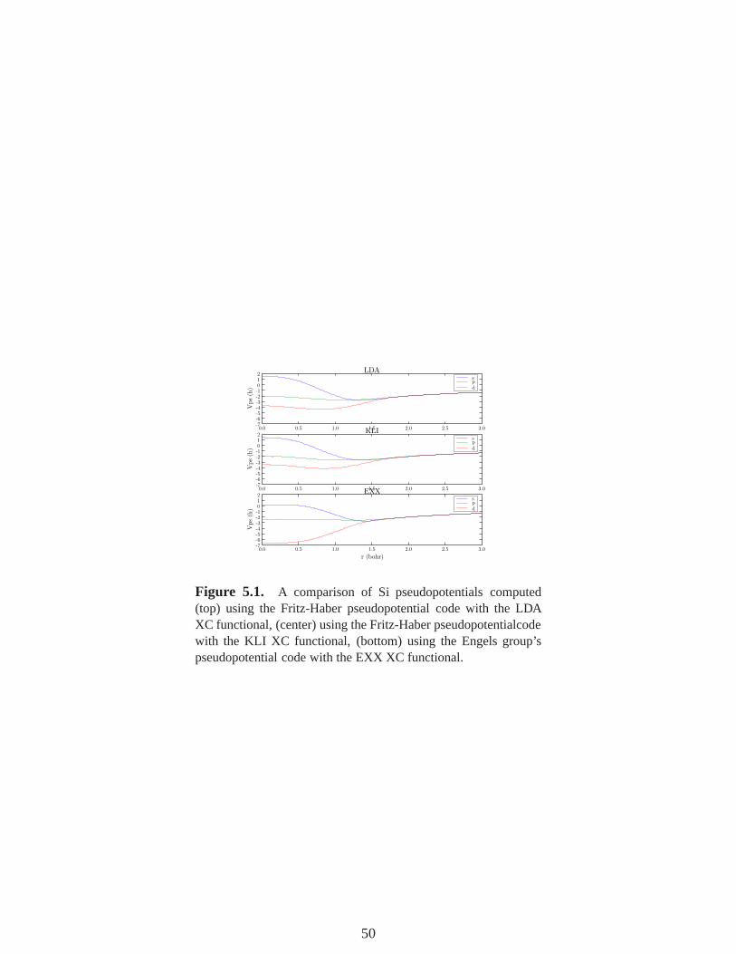
Figure 5.1. A comparison of Si pseudopotentials computed(top) using the Fritz-Haber pseudopotential code with the LDAXC functional, (center) using the Fritz-Haber pseudopotentialcodewith the KLI XC functional, (bottom) using the Engels group’spseudopotential code with the EXX XC functional.

50

Chapter 6

Small system tests of the OEP

We now report the performance of EXX methods on a variety of test systems. We report a compar-ison of a spectrum of excitation energies for Helium and Beryllium atoms, we report the accuracyof the functionals for molecular hydrogen geometries with stretched H–H bond lengths, and wereport the behavior of the band gap of Helium atom at elevated temperatures. These test problemshave been computed using an all-electron EXX method described in reference [22].

Helium Atom

Figure 6.1 shows a comparison of Helium excitation energies to the (essentially exact) QMC-derived exchange-correlation functional as well as to HF and to other LDA, GGA, and Hybridfunctionals. The two methods derived in the current LDRD project, labelledEXX andEXX-GGAin the figure, perform significantly better than the HF method and the other density functionals.The average error of the EXX (0.016 h) and the EXX-GGA (0.014 h) methods is significatly lowerthan that from HF (0.107 h), LDA (0.241 h), GGA (0.227–0.232 h) or hybrid (0.160 h) methods.Furthermore, the EXX values differ from the QMC-derived values by essentially constant valuesacross the entire spectrum, whereas the errors in the other methods fluctuate considerably. As aresult, the EXX methods are the only ones that properly predict the ordering of the excited states.

Beryllium Atom

Figure 6.2 reports a similar comparison for Beryllium atom. On the average the HF excitationenergies differ by 0.075 h, the LDA, BLYP, and PBE values differ by 0.050–0.070, and the B3LYPvalues differ by 0.038 h. In contrast, the EXX values differ by only 0.004 h, nearly a factor of tensmaller average difference than the best of the standard DFTs. Moreover, as was seen in He, theOEP excitation energies differ from the QMC values by a constant shift, whereas the LDA, GGA,and HF values fluctuate much more about their averages. The figure illustrates that not only doesthe EXX perform better on the average, but that each individual excitation value once again differsfrom the exact levels by a small, nearly constant shift.

51

Figure 6.1. A comparison of the excitation energies for differ-ent states of Helium atom, using the Hartree-Fock (HF) method,and density functional theory using the LDA, BLYP, PBE, B3LYPfunctionals, as well as the EXX and EXX-GVB method develop inthis LDRD project.

Figure 6.2. A comparison of the excitation energies for differentstates of Beryllium atom, using the Hartree-Fock (HF) method,and density functional theory using the LDA, BLYP, PBE, B3LYPfunctionals, as well as the EXX method develop in this LDRDproject.

52

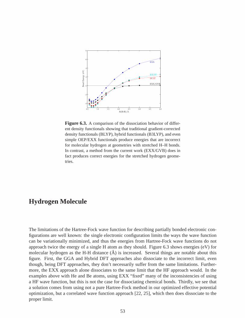
Figure 6.3. A comparison of the dissociation behavior of differ-ent density functionals showing that traditional gradient-correcteddensity functionals (BLYP), hybrid functionals (B3LYP), and evensimple OEP/EXX functionals produce energies that are incorrectfor molecular hydrogen at geometries with stretched H–H bonds.In contrast, a method from the current work (EXX/GVB) does infact produces correct energies for the stretched hydrogen geome-tries.

Hydrogen Molecule

The limitations of the Hartree-Fock wave function for describing partially bonded electronic con-figurations are well known: the single electronic configuration limits the ways the wave functioncan be variationally minimized, and thus the energies from Hartree-Fock wave functions do notapproach twice the energy of a single H atom as they should. Figure 6.3 shows energies (eV) formolecular hydrogen as the H-H distance (A) is increased. Several things are notable about thisfigure. First, the GGA and Hybrid DFT approaches also dissociate to the incorrect limit, eventhough, being DFT approaches, they don’t necessarily suffer from the same limitations. Further-more, the EXX approach alone dissociates to the same limit that the HF approach would. In theexamples above with He and Be atoms, using EXX “fixed” many of the inconsistencies of usinga HF wave function, but this is not the case for dissociating chemical bonds. Thirdly, we see thata solution comes from using not a pure Hartree-Fock method in our optimized effective potentialoptimization, but a correlated wave function approach [22, 25], which then does dissociate to theproper limit.

53

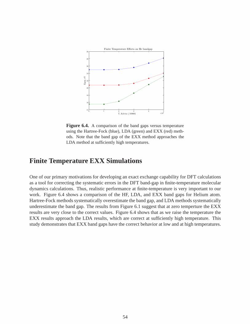
Figure 6.4. A comparison of the band gaps versus temperatureusing the Hartree-Fock (blue), LDA (green) and EXX (red) meth-ods. Note that the band gap of the EXX method approaches theLDA method at sufficiently high temperatures.

Finite Temperature EXX Simulations

One of our primary motivations for developing an exact exchange capability for DFT calculationsas a tool for correcting the systematic errors in the DFT band-gap in finite-temperature moleculardynamics calculations. Thus, realistic performance at finite-temperature is very important to ourwork. Figure 6.4 shows a comparison of the HF, LDA, and EXX band gaps for Helium atom.Hartree-Fock methods systematically overestimate the band gap, and LDA methods systematicallyunderestimate the band gap. The results from Figure 6.1 suggest that at zero temperture the EXXresults are very close to the correct values. Figure 6.4 shows that as we raise the temperature theEXX results approach the LDA results, which are correct at sufficiently high temperature. Thisstudy demonstrates that EXX band gaps have the correct behavior at low and at high temperatures.

54

Chapter 7

Correlation compatible with ExactExchange

In order to explain the necessity of adding a compatible correlation to exact exchange (EXX) wewill use the jellium surface model system in an illustrative example. This model is obtained byperforming a self-consistent LDA calculation on a system where electrons move in an externalpotential of a uniform positively charged background in halfspace. [26] The model itself can beseen as a well-defined procedure to produce densities from which all other quantities can be deter-mined using the Kohn-Sham equations [27] with the LDA exchange-correlation functional. Thenon-homogeneous densities that define the model are expressed in the dimensionless parameterrs = a0(3/(4π)n)1/3, wheren is the density of the positive background, anda0 is the bohr radius.The total system of positive background and electrons is neutral and the bulk electron density,nbulk, far inside the half space positive background is then equal to ¯n. Typical jellium surfacemodel densities are shown in Fig. 7.1.

-20 -15 -10 -5 5za0

0.2

0.4

0.6

0.8

1

nnbulk

Jelliumsurface densities for rs=2.07and5.00

Figure 7.1.Examples of two jellium surface densities with differ-entrs-values.rs = 2.07 corresponds to the valence electron densityin aluminum. Largerrs corresponds to lower density.

55

Table 7.1.Exchange surface energies, in erg/cm2, for the jelliumsurface model. Mean absolute relative errors (mare) are comparedto the EXX results [28].

rs LDA PBE EXX2.00 3036 2436 26242.07 2673 2125 22962.30 1808 1393 15212.66 1051 769 8543.00 668 464 5263.28 477 315 3644.00 222 128 1575.00 92 40 57mare 29% 13% −

For a given jellium surface, that is, density, the only part ofthe energy that changes using differentfunctionals,εxc(r ; [n]), is the exchange-correlation part, so we only examine this part of the energy.An exchange-correlation surface energy is defined by subtracting the energy an equal amount ofelectrons would have had in a uniform electron gas with the bulk density (this is equivalent to theLDA expression):

σxc =

∫

n(z)[εxc(r ; [n])− εLDAxc (nbulk)]dz. (7.1)

This expression can be divided into an exchange and a correlation part,σxc = σx+σc. This divisionis arbitrary, since only the fullσxc is a physical quantity, not the separateσx andσc. We will herefollow the standard division and defineσx as the quantity obtained by insering the EXX functionalinto Eqn. 7.1. The correlation part is defined as ’the rest’ and need to be derived with methodsoutside of DFT. Table 7.1 shows the jellium surface model surface exchange energies for the LDA,PBE, and EXX exchange functionals. The EXX results are from Ref. [28]. EXX being the correctresult, the two other functionals are compared to the EXX results by calculation of the meanabsolute relative error, mare. As is seen, LDA deviates strongly from the correct answer with 29%mare, while PBE is doing better with 13% mare. Taken out of perspective this discrepancy wouldbe sufficient to motivate the use of the much more computationally expensive EXX functional.However, as pointed out before, the physical quantity is the full exchange-correlation energy, notthe separate exchange or correlation energies.

In Tab. 7.2, the surface correlation energies for the same jellium surface model is given. Here theRPA+ is the best available approximation for the exact correlation energy [29]. As seen, also thecorrelation is far off, in particular for LDA with a 63% mare from the RPA+ results. However,combining exchange and correlation into the real physical quantity, results are given in Tab. 7.3,the errors made in exchange and correlation are cancelling to the extent that LDA only has a 2%error and actually is better than PBE, which had both the separate exchange and correlation betterthan LDA. This effect is due to the LDA correlation being ’compatible’ with LDA exchange. Boththe LDA exchange and correlation are derived from a model system, the uniform electron gas, forwhich LDA thus is the correct answer. Applying LDA to a non-uniform electron gas, such as the

56

Table 7.2. Correlation surface energies, in erg/cm2, for the jel-lium surface model. Mean absolute relative errors (mare) are com-pared to the RPA+ results [29].

rs LDA PBE RPA+2.00 317 827 7892.07 287 754 7192.30 210 567 5392.66 136 381 3603.00 95 275 2553.28 72 215 1994.00 39 124 1115.00 19 67 56mare 63% 8% −

jellium surface densities in Fig. 7.1, errors made in exchange has a tendency to cancel with errorsmade in the correlation as is seen in Tabs 7.1-7.3. PBE is not constructed from a model system andthus does not have compatible exchange and correlation, see the tables.

Table 7.3.Exchange-correlation surface energies, in erg/cm2, forthe jellium surface model. Mean absolute relative errors (mare) arecompared to the EXX/RPA+ results.

rs LDA PBE EXX/RPA+2.00 3354 3264 34132.07 2960 2879 30152.30 2019 1960 20602.66 1187 1150 12143.00 763 739 7813.28 549 530 5634.00 261 252 2685.00 111 107 113mare 2% 5% −

So, what correlation should be used for EXX? Let us examine thejellium surface model again. Ifwe use no correlation at all, thus approximating the EXX/RPA+ numbers in Tab. 7.3 with the EXXnumbers in Tab. 7.1, we would make errors between 23 and 50%, with a mare of 33%. Combiningthe EXX in Tab. 7.1 with LDA/PBE correlation in Tab. 7.2 would make errors between 14/1 and33/10%, mare 21/3%. It would thus be reasonable to use PBE correlation together with EXX.This exercise shows that the usual practice of adding no or LDA correlation to EXX results is notwell founded.

We will now proceed and use the jellium surface model system to construct a partially compatible

57

correlation for EXX by parametrizing the RPA+ correlation inTab. 7.2. We will follow approx-imately the same procedure as in [30]. We will use an index dependent on the dimensionlessdensity gradient parameters2 = |∇n|2/(4(3π2)2/3n8/3) to interpolating between ’interior’ (s= 0,LDA correlation, index=1) and edge region (s→ ∞, index=0):

XIDX(s2) = 1−cs2/(cs2+1) (7.2)

FIDX(s2) = 2/(1+exp(s2/t)) (7.3)

These two possible indices are shown in Fig. 7.2, for the values ofc and t obtained in the fitsdescribed below. TheXIDX index is used in the am05 functional[30].

0.5 1 1.5 2s2

0.2

0.4

0.6

0.8

1IDX

XIDX Hc=1.4805, blueLFIDX Ht=0.3123, redL

Figure 7.2. Examples of two possible indices to interpolate be-tween ’interior’ (LDA correlation, index=1) and edge region (in-dex=0) .

For the interior region, far from the surface, where the density is slowly varying (see Fig. 7.1),LDA correlation (LDAc) is a suitable functional. For the edge region we will use a scaled LDAcorrelation, with the scaling set by fitting. The two correlation functionals we here construct thushave the following form:

EXXc(n,s) = IDX(s2)∗LDAc(n)+(1− IDX(s2))∗ (g1+g2∗ rs(n))∗LDAc(n) , (7.4)

where IDX is eitherXIDX or FIDX from Eqn. 7.3, andg1 and g2 are fitting constants. Notealso thatrs here is calculated from the local density, not the bulk/positive background density asabove. In the construction of am05 [30] only one scaling constant,g1, was used, but to accuratelyrepresent the RPA+ data in Tab. 7.2, two fitting constants are needed. Also note that we correctlywould obtain the LDAc for a uniform electron gas system wheres2 = 0, sinceIDX(0) = 1 byconstruction.

58

The constants,(g1,g2,c) for EXXXcand(g1,g2, t) for EXXFc, are fitted by non-linear fitting tothe RPA+ data in Tab. 7.2. In this case we use the PW parametrization [31] of the LDAc. ThePZ correlation [32] would be equally suitable but would give slightly different values of the fittingparameters. Both forms of the index give equally good fits and reproduces the RPA+ results inTab. 7.2 to within error bars (±1 erg/cm2). The constants take the values

EXXXc : (g1,g2,c) = (0.02245,0.03672,1.4805) , (7.5)

EXXFc : (g1,g2, t) = (0.3060,0.04108,0.3123) . (7.6)

In order to compare the two here created correlation functionals with GGA correlations (PBEc [33]and PW91c [34]) and the PW [31] and PZ [32] parametrizations of Ceperley and Alder’s MonteCarlo derived LDA correlation [35], we examine the accumulated surface correlation energy ob-tained from the correlation part of the integrand in Eqn. 7.1 integrated from−∞ to z. This accumu-lated surface correlation energy is shown in Fig. 7.3 for the same twors values as in Fig. 7.1. It isclearly seen that scaling the LDA correlation in the edge region makesEXXXcandEXXFcbehavelike the GGA correlations even though the derivation of the here presented correlation functionalshas nothing in common with the derivation of the PBEc and PW91c. We also see that the maindifference from the GGA correlations is picked up outside of the surface. It is also interesting tonote that despite that the indices in Eqn. 7.3 are quite different (see also Fig. 7.2) the final resultsare very similar. A final, obvious, observation is that the accumulated surface correlation indeedconverge towards the RPA+ values that the full integrals were fitted to.

We have constructed two correlation functionals that reproduce the correct correlation in two modelsystems, the uniform electron gas and the jellium surface system. This correlation is thus par-tially compatible with EXX. The two correlation functionals seems to reproduce GGA results formoderate values ofs2. Full and realistic testing is needed before any final conclusions about theperformance of these two correlation functionals can be made.

59

-4 -2 2 4 6 8z

100

200

300

400

500

600

700

integrated from -¥ to z

Accumulated surface correlation energy for rs=2.07 HAlL.PW HblackL, PZ HvioletL, PBEc HgreenL,PW91c Hlight greenL, EXXXc HblueL, and EXXFc HredL.Dashed line is RPA+.

(a) rs = 2.07.

-4 -2 2 4 6 8z

10

20

30

40

50

60

integrated from -¥ to z

Accumulated surface correlation energy for rs=5.PW HblackL, PZ HvioletL, PBEc HgreenL,PW91c Hlight greenL, EXXXc HblueL, and EXXFc HredL.Dashed line is RPA+.

(b) rs = 5.00.

Figure 7.3.Accumulated surface correlation energy.

60

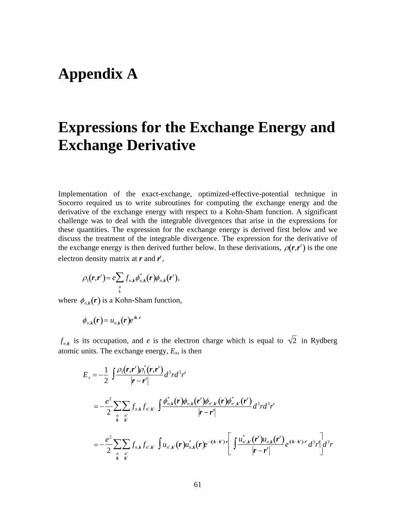
Appendix A Expressions for the Exchange Energy and Exchange Derivative Implementation of the exact-exchange, optimized-effective-potential technique in Socorro required us to write subroutines for computing the exchange energy and the derivative of the exchange energy with respect to a Kohn-Sham function. A significant challenge was to deal with the integrable divergences that arise in the expressions for these quantities. The expression for the exchange energy is derived first below and we discuss the treatment of the integrable divergence. The expression for the derivative of the exchange energy is then derived further below. In these derivations, ρ r, ′ r ( ) is the one electron density matrix at r and r′, ρ1 r, ′ r ( )= e fn,kφn,k

* r( )φn,k ′ r ( )nk

∑ ,

where φn,k r( ) is a Kohn-Sham function, φn,k r( )= un,k r( )eik ⋅r fn ,k is its occupation, and e is the electron charge which is equal to 2 in Rydberg

atomic units. The exchange energy, Ex, is then

Ex = −12

ρ1 r, ′ r ( )ρ1* r, ′ r ( )

r − ′ r d3rd3 ′ r ∫

= −e2

2fn,k f ′ n , ′ k

φn,k* r( )φn,k ′ r ( )φ ′ n , ′ k r( )φ ′ n , ′ k

* ′ r ( )r − ′ r

d3rd3 ′ r ∫′ n ′ k

∑nk

∑

= −e2

2fn,k f ′ n , ′ k u ′ n , ′ k r( )un,k

* r( )∫′ n ′ k

∑nk

∑ e− i k− ′ k ( )⋅r u ′ n , ′ k * ′ r ( )un,k ′ r ( )

r − ′ r ei k− ′ k ( )⋅ ′ r d3 ′ r ∫

⎡

⎣ ⎢

⎤

⎦ ⎥ d3r

61

= −e2

2fn,k f ′ n , ′ k h ′ n , ′ k ,n,k

* r( )∫′ n ′ k

∑nk

∑ e−i k− ′ k ( )⋅r h ′ n , ′ k ,n,k ′ r ( )r − ′ r

ei k− ′ k ( )⋅ ′ r ∫ d3 ′ r ⎡

⎣ ⎢

⎤

⎦ ⎥ d3r

= −e2

2fn,k f ′ n , ′ k h ′ n , ′ k ,n,k

* r( )∫′ n ′ k

∑nk

∑ e−i k− ′ k ( )⋅r h ′ n , ′ k ,n,k G( )G∑ ei k− ′ k +G( )⋅ ′ r

r − ′ r ∫ d3 ′ r ⎡

⎣ ⎢

⎤

⎦ ⎥ d3r

= −2πe2 fn ,k f ′ n , ′ k h ′ n , ′ k ,n,k* r( )∫

′ n ′ k

∑nk

∑ e−i k− ′ k ( )⋅r h ′ n , ′ k ,n ,k G( )k − ′ k + G 2 ei k− ′ k +G( )⋅r

G∑

⎡

⎣ ⎢ ⎢

⎤

⎦ ⎥ ⎥ d3r

= −2πe2 fn ,k f ′ n , ′ k h ′ n , ′ k ,n,k* r( )∫

′ n ′ k

∑nk

∑ h ′ n , ′ k ,n ,k G( )k − ′ k + G 2 eiG⋅r

G∑

⎡

⎣ ⎢ ⎢

⎤

⎦ ⎥ ⎥ d 3r

= −2πe2 fn,k f ′ n , ′ k h ′ n , ′ k ,n,k* r( )∫

′ n ′ k

∑nk

∑ H ′ n , ′ k ,n,k G( )eiG⋅r

G∑

⎡

⎣ ⎢

⎤

⎦ ⎥ d3r

= −2πe2 fn ,k f ′ n , ′ k h ′ n , ′ k ,n,k

* r( )∫′ n ′ k

∑nk

∑ H ′ n , ′ k ,n,k r( )d3r

We next discuss the treatment of the integrable divergence that appears in this

expression. In DFT plane wave calculations, un,k r( ) is normalized over a cell volume (Ω) and is constrained to be orthogonal to u ′ n ,k r( ) when n′ ≠ n. As such, the integrals of

and over the cell volume − h ′ n = n ,k,n ,k r( ) h ′ n ≠n ,k,n ,k r( ) h ′ n = n,k,n ,k G = 0( ) and − have the values 1 and 0, respectively. In the latter case, the terms will also be equal to 0 and the numerical problem of dividing by

h ′ n ≠n ,k,n,k G = 0( )H ′ n ≠n,k ,n,k G = 0( )

G 2 = 0 is avoided by skipping them. In the former case, the terms H ′ n = n,k ,n,k G = 0( ) are undefined and thus require special treatment. To treat these terms, I begin by separating them from the others:

fn,k f ′ n , ′ k h ′ n , ′ k ,n,k* r( )∫

′ n ′ k

∑nk

∑ H ′ n , ′ k ,n,k G( )eiG⋅r

G∑

⎡

⎣ ⎢

⎤

⎦ ⎥ d3r

62

= fn,k f ′ n , ′ k h ′ n , ′ k ,n,k* r( )∫

′ n ′ k ≠k

∑nk

∑ H ′ n , ′ k ,n,k G( )eiG⋅r

G∑

⎡

⎣ ⎢

⎤

⎦ ⎥ d3r

+ fn,k f ′ n ,k h ′ n ,k,n,k* r( )∫

′ n ∑

nk

∑ H ′ n ,k,n,k G( )eiG⋅r

G∑

⎡

⎣ ⎢

⎤

⎦ ⎥ d3r

= fn,k f ′ n , ′ k h ′ n , ′ k ,n,k* r( )∫

′ n ′ k ≠k

∑nk

∑ H ′ n , ′ k ,n,k G( )eiG⋅r

G∑

⎡

⎣ ⎢

⎤

⎦ ⎥ d3r

+ fn,k f ′ n ,k h ′ n ,k,n,k* r( )∫

′ n ≠n∑

nk

∑ H ′ n ,k,n,k G( )eiG⋅r

G∑

⎡

⎣ ⎢

⎤

⎦ ⎥ d3r

+ fn,k fn,k hn,k,n,k* r( )∫ Hn,k,n,k G( )eiG⋅r

G∑

⎡

⎣ ⎢

⎤

⎦ ⎥ d3r

nk

∑

= fn,k f ′ n , ′ k h ′ n , ′ k ,n,k* r( )∫

′ n ′ k ≠k

∑nk

∑ H ′ n , ′ k ,n,k G( )eiG⋅r

G∑

⎡

⎣ ⎢

⎤

⎦ ⎥ d3r

+ fn,k f ′ n ,k h ′ n ,k,n,k* r( )∫

′ n ≠n∑

nk

∑ H ′ n ,k,n,k G( )eiG⋅r

G≠0∑

⎡

⎣ ⎢

⎤

⎦ ⎥ d3r

+ fn,k fn,k hn,k,n,k* r( )∫ Hn,k,n,k G( )eiG⋅r

G≠0∑

⎡

⎣ ⎢

⎤

⎦ ⎥ d3r

nk

∑

+ fn,k fn,k Hn,k,n,k G = 0( )[ ] hn,k,n,k* r( )∫ d3r

nk

∑

= fn,k f ′ n , ′ k h ′ n , ′ k ,n,k* r( )∫

′ n ′ k ≠k

∑nk

∑ H ′ n , ′ k ,n,k G( )eiG⋅r

G∑

⎡

⎣ ⎢

⎤

⎦ ⎥ d3r

+ fn,k f ′ n ,k h ′ n ,k,n,k* r( )∫

′ n ∑

nk

∑ H ′ n ,k,n,k G( )eiG⋅r

G≠0∑

⎡

⎣ ⎢

⎤

⎦ ⎥ d3r

+ fn,k fn,k Hn,k,n,k G = 0( )[ ] hn,k,n,k* r( )∫ d3r

nk

∑

The divergent terms are in the final sum in the expression above. Gygi and

Baldereschi [PRB 34, 4405 (1986)] noted similar divergent terms in their expressions for the matrix elements of the Hartree-Fock exchange operator in the reciprocal space

63

representation. They noted that the divergence is integrable in that the analytic integral of over the Brillouin zone is finite. Given this, they replaced the divergent

terms as shown below: Hn,k,n,k G = 0( )

Hn,k,n,k G = 0( )= hn,k,n,k G = 0( ) F q( )dqBZ∫ − F k − ′ ′ k ( )

′ ′ k ≠k∑

⎧ ⎨ ⎩

⎫ ⎬ ⎭

= hn,k,n,k G = 0( ) F q( )dqBZ∫ − F ′ ′ k ( )

′ ′ k ≠0∑

⎧ ⎨ ⎩

⎫ ⎬

⎭ where F is a function which is periodic in reciprocal space, has the same type (i.e. q −2 ) of divergence as , and is sufficiently smooth that it can be numerically integrated using a modest number of points in the Brillouin zone. I note that the k-point mesh used to perform the (partial) numerical integration of F does not have to be the same mesh on which the wave functions are computed. As such, this replacement allows for calculations at a single k-point in the Brillouin zone. The expression given above for the exchange energy is then written as

Hn,k,n,k G = 0( )

Ex = −2πe2 fn,k f ′ n , ′ k h ′ n , ′ k ,n,k* r( )∫

′ n ′ k ≠k

∑nk

∑ H ′ n , ′ k ,n,k G( )eiG⋅r

G∑

⎡

⎣ ⎢

⎤

⎦ ⎥ d3r

⎧

⎨ ⎪

⎩ ⎪

+ fn,k f ′ n ,k h ′ n ,k,n,k* r( )∫

′ n ∑

nk

∑ H ′ n ,k,n,k G( )eiG⋅r

G≠0∑

⎡

⎣ ⎢

⎤

⎦ ⎥ d3r

+ fn,k fn,khn,k,n,k G = 0( ) F q( )dqBZ∫ − F ′ ′ k ( )

′ ′ k ≠0∑

⎡

⎣ ⎢

⎤

⎦ ⎥ hn,k,n,k

* r( )∫ d3rnk

∑⎫

⎬ ⎪

⎭ ⎪

= −2πe2 fn,k f ′ n , ′ k h ′ n , ′ k ,n,k* r( )∫ H ′ n , ′ k ,n,k r( )

′ n ′ k ≠k

∑nk

∑ d3r⎧

⎨ ⎪

⎩ ⎪

+ fn,k f ′ n ,k h ′ n ,k,n,k* r( ) ˜ H ′ n ,k,n,k r( )∫

′ n ∑

nk

∑ d3r

+ fn,k fn,k hn,k,n,k G = 0( )2

F q( )dqBZ∫ − F ′ ′ k ( )

′ ′ k ≠0∑

⎡

⎣ ⎢

⎤

⎦ ⎥

nk

∑⎫

⎬ ⎪

⎭ ⎪

64

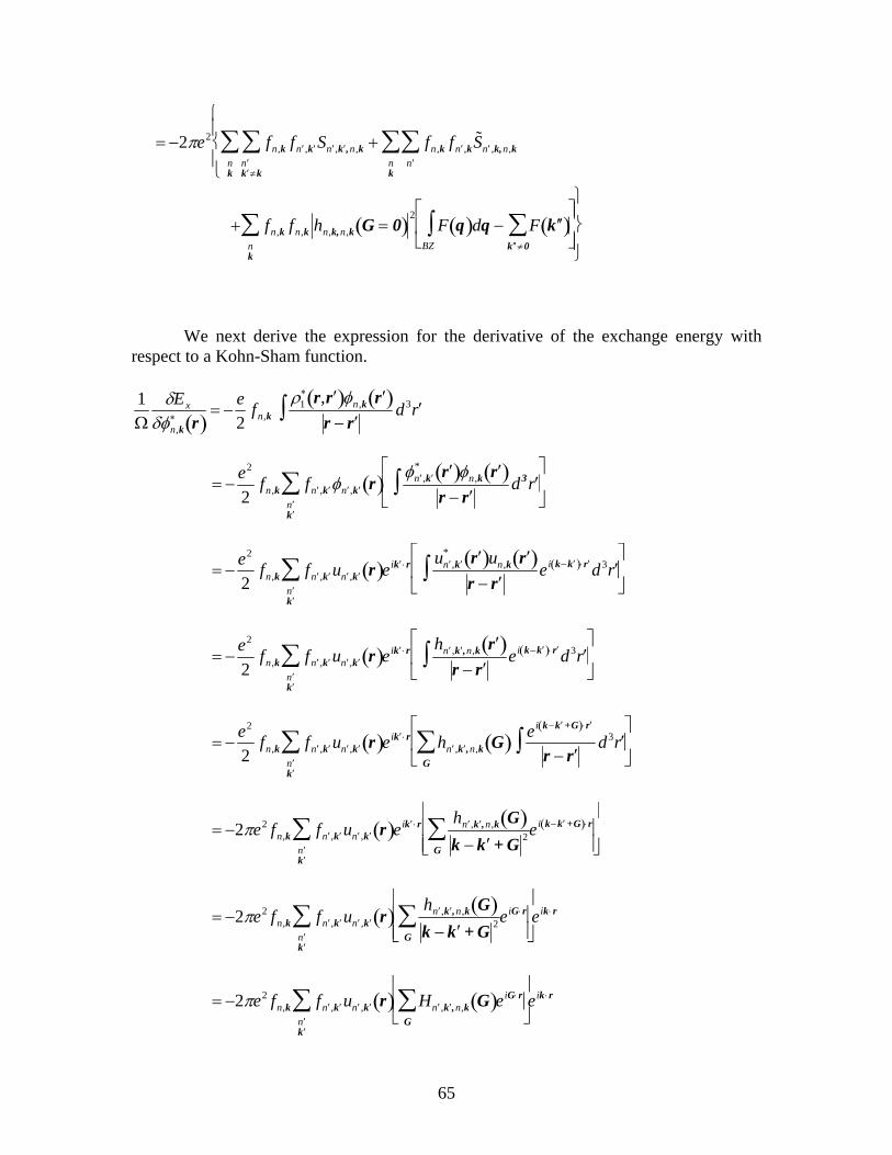
= −2πe2 fn,k f ′ n , ′ k S ′ n , ′ k ,n,k′ n ′ k ≠k

∑nk

∑ + fn,k f ′ n ,k′ n

∑nk

∑ ˜ S ′ n ,k,n,k

⎧

⎨ ⎪

⎩ ⎪

+ fn,k fn,k hn,k,n,k G = 0( )2

F q( )dqBZ∫ − F ′ ′ k ( )

′ ′ k ≠0∑

⎡

⎣ ⎢

⎤

⎦ ⎥

nk

∑⎫

⎬ ⎪

⎭ ⎪

We next derive the expression for the derivative of the exchange energy with respect to a Kohn-Sham function. 1Ω

δEx

δφn,k∗ r( )

= −e2

fn,kρ1

∗ r, ′ r ( )φn,k ′ r ( )r − ′ r

d3 ′ r ∫

= −e2

2fn,k f ′ n , ′ k φ ′ n , ′ k r( ) φ ′ n , ′ k

* ′ r ( )φn,k ′ r ( )r − ′ r

d3 ′ r ∫⎡

⎣ ⎢

⎤

⎦ ⎥

′ n ′ k

∑

= −e2

2fn,k f ′ n , ′ k u ′ n , ′ k r( )ei ′ k ⋅r u ′ n , ′ k

* ′ r ( )un,k ′ r ( )r − ′ r

ei k− ′ k ( )⋅ ′ r d3 ′ r ∫⎡

⎣ ⎢

⎤

⎦⎥

′ n ′ k

∑

= −e2

2fn,k f ′ n , ′ k u ′ n , ′ k r( )ei ′ k ⋅r h ′ n , ′ k ,n,k ′ r ( )

r − ′ r ei k− ′ k ( )⋅ ′ r d3 ′ r ∫

⎡

⎣ ⎢

⎤

⎦⎥

′ n ′ k

∑

= −e2

2fn,k f ′ n , ′ k u ′ n , ′ k r( )ei ′ k ⋅r h ′ n , ′ k ,n,k G( )

G∑ ei k− ′ k +G( )⋅ ′ r

r − ′ r d3 ′ r ∫

⎡

⎣ ⎢

⎤

⎦ ⎥

′ n ′ k

∑

= −2πe2 fn,k f ′ n , ′ k u ′ n , ′ k r( )ei ′ k ⋅r h ′ n , ′ k ,n,k G( )k − ′ k + G 2

G∑ ei k− ′ k +G( )⋅r

⎡

⎣ ⎢ ⎢

⎤

⎦ ⎥ ⎥ ′ n

′ k

∑

= −2πe2 fn,k f ′ n , ′ k u ′ n , ′ k r( ) h ′ n , ′ k ,n,k G( )k − ′ k + G 2

G∑ eiG⋅r

⎡

⎣ ⎢ ⎢

⎤

⎦ ⎥ ⎥ ′ n

′ k

∑ eik⋅r

= −2πe2 fn,k f ′ n , ′ k u ′ n , ′ k r( ) H ′ n , ′ k ,n,k G( )eiG⋅r

G∑

⎡

⎣ ⎢

⎤

⎦ ⎥

′ n ′ k

∑ eik⋅r

65

= −2πe2 fn,k f ′ n , ′ k u ′ n , ′ k r( )H ′ n , ′ k ,n,k r( )

′ n ′ k

∑ eik ⋅r

Then 1Ω

δEx

δun,k∗ r( )

= −2πe2 fn,k f ′ n , ′ k u ′ n , ′ k r( )H ′ n , ′ k ,n,k r( )′ n ′ k

∑

The treatment of the integrable divergence in this expression proceeds in the same way as noted above for the exchange energy. I begin by separating the divergent term from the others:

f ′ n , ′ k u ′ n , ′ k r( ) H ′ n , ′ k ,n,k G( )eiG⋅r

G∑

⎡

⎣ ⎢

⎤

⎦ ⎥

′ n ′ k

∑

= f ′ n , ′ k u ′ n , ′ k r( ) H ′ n , ′ k ,n,k G( )eiG⋅r

G∑

⎡

⎣ ⎢

⎤

⎦ ⎥

′ n ′ k ≠k

∑ + f ′ n ,ku ′ n ,k r( )′ n

∑ H ′ n ,k,n,k G( )eiG⋅r

G∑

⎡

⎣ ⎢

⎤

⎦ ⎥

= f ′ n , ′ k u ′ n , ′ k r( ) H ′ n , ′ k ,n ,k G( )eiG⋅r

G∑

⎡

⎣ ⎢

⎤

⎦ ⎥

′ n ′ k ≠k

∑ + f ′ n ,ku ′ n ,k r( )′ n ≠n∑ H ′ n ,k,n,k G( )eiG⋅r

G∑

⎡

⎣ ⎢

⎤

⎦ ⎥

+ fn ,kun,k r( ) Hn,k,n ,k G( )eiG⋅r

G∑

⎡

⎣ ⎢

⎤

⎦ ⎥

= f ′ n , ′ k u ′ n , ′ k r( ) H ′ n , ′ k ,n ,k G( )eiG⋅r

G∑

⎡

⎣ ⎢

⎤

⎦ ⎥

′ n ′ k ≠k

∑ + f ′ n ,ku ′ n ,k r( )′ n ≠n∑ H ′ n ,k,n,k G( )eiG⋅r

G≠0∑

⎡

⎣ ⎢

⎤

⎦ ⎥

+ fn ,kun,k r( ) Hn,k,n ,k G( )eiG⋅r

G≠0∑

⎡

⎣ ⎢

⎤

⎦ ⎥ + fn,kun ,k r( )Hn,k,n ,k G = 0( )

= f ′ n , ′ k u ′ n , ′ k r( ) H ′ n , ′ k ,n,k G( )eiG⋅r

G∑

⎡

⎣ ⎢

⎤

⎦ ⎥

′ n ′ k ≠k

∑ + f ′ n ,ku ′ n ,k r( )′ n

∑ H ′ n ,k,n,k G( )eiG⋅r

G≠0∑

⎡

⎣ ⎢

⎤

⎦ ⎥

+ fn,kun,k r( )Hn ,k,n,k G = 0( )

The divergent term is in the final sum in the expression above. As explained

above, Gygi and Baldereschi [PRB 34, 4405 (1986)] noted similar divergent terms in their expressions for the matrix elements of the Hartree-Fock exchange operator in the reciprocal space representation. They further noted that the divergence is integrable in

66

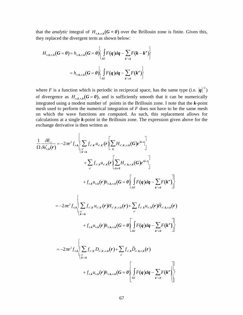
that the analytic integral of Hn,k ,n,k G = 0( ) over the Brillouin zone is finite. Given this, they replaced the divergent term as shown below:

Hn,k,n ,k G = 0( )= hn,k,n ,k G = 0( ) F q( )dqBZ∫ − F k − ′ ′ k ( )

′ ′ k ≠k∑

⎧ ⎨ ⎩

⎫ ⎬ ⎭

= hn,k,n,k G = 0( ) F q( )dqBZ∫ − F ′ ′ k ( )

′ ′ k ≠0∑

⎧ ⎨ ⎩

⎫ ⎬ ⎭

where F is a function which is periodic in reciprocal space, has the same type (i.e. q −2 ) of divergence as , and is sufficiently smooth that it can be numerically integrated using a modest number of points in the Brillouin zone. I note that the k-point mesh used to perform the numerical integration of F does not have to be the same mesh on which the wave functions are computed. As such, this replacement allows for calculations at a single k-point in the Brillouin zone. The expression given above for the exchange derivative is then written as

Hn,k ,n,k G = 0( )

1Ω

δEx

δun,k∗ r( )

= −2πe2 fn,k f ′ n , ′ k u ′ n , ′ k r( ) H ′ n , ′ k ,n,k G( )eiG⋅r

G∑

⎡

⎣ ⎢

⎤

⎦ ⎥

′ n ′ k ≠k

∑⎧

⎨ ⎪

⎩ ⎪

+ f ′ n ,ku ′ n ,k r( )′ n

∑ H ′ n ,k,n,k G( )eiG⋅r

G≠0∑

⎡

⎣ ⎢

⎤

⎦ ⎥

+ fn,kun,k r( )hn,k,n,k G = 0( ) F q( )dqBZ∫ − F ′ ′ k ( )

′ ′ k ≠0∑

⎡

⎣ ⎢

⎤

⎦ ⎥ ⎫ ⎬ ⎭

= −2πe2 fn,k f ′ n , ′ k u ′ n , ′ k r( )H ′ n , ′ k ,n,k r( )′ n ′ k ≠k

∑⎧

⎨ ⎪

⎩ ⎪

+ f ′ n ,ku ′ n ,k r( ) ˜ H ′ n ,k,n,k r( )′ n

∑

+ fn,kun,k r( )hn,k,n,k G = 0( ) F q( )dqBZ∫ − F ′ ′ k ( )

′ ′ k ≠0∑

⎡

⎣ ⎢

⎤

⎦ ⎥ ⎫ ⎬ ⎭

= −2πe2 fn,k f ′ n , ′ k D ′ n , ′ k ,n,k r( )+ f ′ n ,k˜ D ′ n ,k,n,k r( )

′ n ∑

′ n ′ k ≠k

∑⎧

⎨ ⎪

⎩ ⎪

+ fn,kun,k r( )hn,k,n,k G = 0( ) F q( )dqBZ∫ − F ′ ′ k ( )

′ ′ k ≠0∑

⎡

⎣

⎢ ⎢ ⎢

⎤

⎦

⎥ ⎥ ⎥

⎫

⎬ ⎪

⎭

⎪

67

To complete this section, we comment on the possibility of alaising errors. Note

that whereas for un,k G( )= 0 G > Gmax , h ′ n , ′ k ,n,k G( ) and H ′ n , ′ k ,n,k G( ) can be non-zero for G ≤ 2Gmax and can be non-zero for D ′ n , ′ k ,n,k G( ) G ≤ 3Gmax . Furthermore, the mesh typically used in a DFT plane wave calculation is only able to resolve functions having non-zero Fourier coefficients for G ≤ 2Gmax . As such, D ′ n , ′ k ,n,k r( ) will not be resolved and will therefore contain aliasing errors for D ′ n , ′ k ,n,k G( ) Gmax < G ≤ 2Gmax . This is not a problem in practice because only D ′ n , ′ k ,n,k G( ) for G ≤ Gmax are needed to update un,k G( ) and these coefficients do not contain aliasing errors. (The same comments apply to LDA and GGA exchange derivatives.)

68

References

[1] M. P. Desjarlais, J. D. Kress, and L. A. Collins, Phys. Rev. E66, 025401 (2002).

[2] M. P. Desjarlais, Phys. Rev. B68, 064204 (2003).

[3] S. Mazevet, M. P. Desjarlais, L. A. Collins, J. D. Kress, and N. H. Magee, Phys. Rev. E71,016409 (2005).

[4] T. R. Mattsson and M. P. Desjarlais, Phys. Rev. Lett.97, 017801 (2006).

[5] W. L. Kohn and L. J. Sham, Phys. Rev.140, A1133 (1965).

[6] P. Hohenberg and W. Kohn, Phys. Rev.136, B864 (1964).

[7] J. D. Talman and W. F. Shadwick, Phys. Rev. A14, 36 (1976).

[8] V. Sahni, J. Gruenebaum, and J. P. Perdew, Phys. Rev. B26, 4371 (1982).

[9] E. Engel and S. H. Vosko, Phys. Rev. A47, 2800 (1993); Phys. Rev. B50, 10498 (1994).

[10] A. Gorling and M. Levy, Phys. Rev. A50, 196 (1994).

[11] T. Kotani, Phys. Rev. Lett.74, 2989 (1995).

[12] M. Stadele, J. A. Majewski, P. Vogl, and A. Gorling, Phys. Rev. Lett.79, 2089 (1997); M.Stadele, M. Moukara, J. A. Majewski, P. Vogl, and A. Gorling, Phys. Rev. B59, 10031 (1999).

[13] A. Gorling, Phys. Rev. Lett.83, 5459 (1999).

[14] R. Hyman, M. Stiles, , and A. Zangwill. A gradient search method for orbital-dependentcharge-density and current density functional calculations.Phys. Rev. B, 62(23):15521–15526,2000.

[15] S. Kummel and J. P. Perdew. Simple iterative construction of the optimized effective potentialfor orbital functionals, including exact exchange.Phys. Rev. Letters, 90(4):043004, 2003.

[16] R. A. Lippert, N. A. Modine, and A. F. Wright. The optimized effective potential with finitetemperature.J. Phys.: Condens. Matter, 18(17):4295, 2006.

[17] R. A. Horn and C. R. Johnson.Topics in Matrix analysis. Cambridge University Press,Cambridge, 1991.

[18] C. C. Paige and M. A. Saunders. Solution of sparse indefinite systems of linear equations.SIAM J. Numer. Anal., 12:617–629, 1975.

69

[19] G. H. Golub and C. F. V. Loan.Matrix Computations. Johns Hopkins University Press,Baltimore, Maryland, 2d edition, 1989.

[20] V. N. Staroverov, G. E. Scuseria, and E. R. Davidson. Optimized effective potentials yieldingHartree-Fock energies and densities.J. Chem. Phys., 124(14):141103, 2006.

[21] Martin Fuchs and Matthias Scheffler. Ab initio pseudopotentials for electronic structurecalculations of poly-atomic systems using density functional theory.Comp. Phys. Comm.,119:67–98, 1999.

[22] Richard P. Muller and Michael P. Desjarlais. Optimized effective potential from a correlatedwave function: Optimized effective potential-generalized valence bond (OEP-GVB).J. Chem.Phys., 125:54101, 2006.

[23] M. Moukara, M. Stadele, J. A. Majewski, P. Vogl, and A. Goerling. Norm-conservingpseudopotentials in the exact-exchange Kohn-Sham formalism.J. Phys.: Condens. Matter,12:6783–6798, 2000.

[24] E. Engel, A. Hock, R. N. Schmid, R. M. Dreizler, and N. Chetty. Role of the core-valenceinteraction for pseudopotential calculations with exact exchange.Phys. Rev. B, 64:125111,2001.

[25] Frank W. Bobrowicz and William A. Goddard, III. The self-consistent field equations for gen-eralized valence bond and open-shell Hartree-Fock wave functions. In Henry F. Schaefer, III,editor,Methods of Electronic Structure Theory, volume 3 ofModern Theoretical Chemistry,page 79. Plenum Press, New York, 1977.

[26] N. D. Lang and W. Kohn, ”Theory of Metal Surfaces: Charge Density and Surface Energy”,Physical Review B1, 4555 (1970).

[27] W. Kohn and L. J. Sham, ”Self-Consistent Equations Including Exchange and CorrelationEffects”, Physical Review140, A1133 (1964).

[28] J. M. Pitarke and A. G. Eguiluz, ”Jellium surface energy beyond the local-density approxi-mation: Self-consistent-field calculations”, Physical Review B63, 045116 (2001).

[29] Z. Yan, J. P. Perdew, and S. Kurth, ”Density functional for short-range correlation: Accuracyof the random-phase approximation for isoelectronic energy changes”, Physical Review B61,16430 (2000).

[30] R. Armiento and A. E. Mattsson, ”Functional designed to include surface effects in self-consistent density functional theory”, Physical Review B72, 085108 (2005).

[31] J. P. Perdew and Y. Wang, ”Accurate and simple analytic representation of the electron-gascorrelation energy”, Physical Review B45, 13244 (1992).

[32] J. P. Perdew and A. Zunger, ”Self-interaction correction to density-functional approximationsfor many-electron systems”, Physical Review B23, 5048 (1981).

70

[33] J. P. Perdew, K. Burke, and M. Ernzerhof, ”Generalized Gradient Approximation MadeSimple”, Physical Review Letters77 3865 (1996).

[34] J. P. Perdew, J. A. Chevary, S. H. Vosko, K. A. Jackson, M. R. Pederson, D. J. Singhi, andC. Fiolhais, ”Atoms, molecules, solids, and surfaces: Applications of the generalized gradientapproximation for exchange and correlation”, Physical Review B46, 6671 (1992).

[35] D. M. Ceperley and B. J. Alder, ”Ground State of the Electron Gas by a Stochastic Method”,Physical Review Letters45, 566 (1980).

71

DISTRIBUTION:

1 MS 1181 Tom Mehlhorn, 1640

2 MS 1186 Mike Desjarlais, 1640

1 MS 1322 Rick Muller, 1435

1 MS 1322 Ann Mattsson, 1435

1 MS 1322 Mark Sears, 1435

1 MS 1415 Alan Wright, 1112

1 MS 1415 Normand Modine, 1132

2 MS 9018 Central Technical Files, 8944

2 MS 0899 Technical Library, 4536

1 MS 0123 D. Chavez, LDRD Office, 1011

72