best practices for implementation and analysis … · best practices for implementation and...

BEST PRACTICES FOR IMPLEMENTATION AND ANALYSIS OF PAIN SCALE PATIENT

REPORTED OUTCOMES IN CLINICAL TRIALS

Nan Shao, Ph.D.Director, Biostatistics

Premier Research Gro p LimitedPremier Research Group, Limited

and

Mark Jaros, Ph.D.Senior Director, Biostatistics

P i R h G Li it dPremier Research Group, Limited

Outline

• During this presentation we will provide some insight on the use of pain scale Patient Reported Outcomes:• Introduction• Variables Measured• Derived Variables

I t ti T h i• Imputation Techniques• Analysis Techniques• Concluding RemarksConcluding Remarks• References Cited

Introduction

• From the FDA Guidance on Patient-Reported Outcomes (PRO): A PRO is a measurement of any aspect of a patient’s health status that comes directly f h i (i i h h i i f h from the patient (i.e., without the interpretation of the patient’s response by a physician or anyone else).

• PRO variables are commonly utilized in acute and chronic pain studies.

• There is variation in the question ‘prompt’ in practice.

Common Acute (A) and Chronic (C) Pain PROs: Instruments applied for assessing PainPROs: Instruments applied for assessing Pain

• Pain Intensity (PI): VAS – (A & C)• PI: Categorical – (A & C)• PI: NPRS – (A & C)• Pain Relief (PR) – (A only)• Global Assessment of Study Medication – (A & C)• Quality of Analgesia – (A & C)• Patient Global Impression of Change (PGIC) – (A & C)• Patient Global Impression of Change (PGIC) – (A & C)• Time to Perceptible (PPR) and Meaningful Pain Relief (MPR) – (A only)• Brief Pain Inventory (BPI) – (A & C)• SF QOL Questionnaires – (C only)• WOMAC Osteoarthritis Index – (C only)• McGill Pain Questionnaire – (A & C)

Pain Intensity (PI) - Visual Analogy Scale (VAS)(VAS)

• Prompt:• How severe is your pain (either at rest or after aggravated

movement [cough])?

• Response:• Response:• Pain Intensity will be measured on a horizontal 100-mm

VAS scale labeled: No Pain (0 mm) as the left anchor and Worst Pain Imaginable (100 mm) as the right anchor. The patient will draw a vertical mark on the line to indicate his pain intensity pain intensity.

PI – Categorical


movement [cough])?

• Response:• Response:• Scored on a 4-point scale (0 = none, 1 = mild,

2 = moderate, 3 = severe)

PI - Numerical Pain Rating Scale (NPRS)


movement [cough])?

• Response:• Response:• Scored on an 11-point numerical scale (0 = no pain and

10 = worst pain)

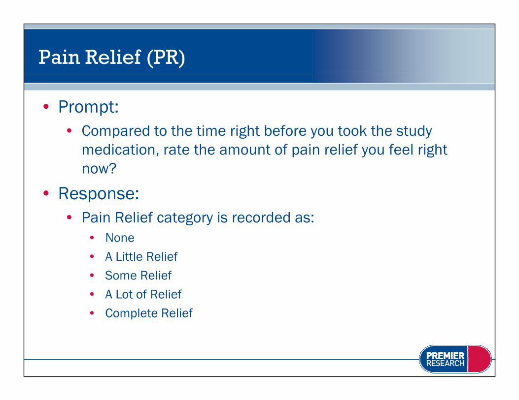
Pain Relief (PR)

• Prompt:• Compared to the time right before you took the study

medication, rate the amount of pain relief you feel right now?

• Response:• Pain Relief category is recorded as: g

• None• A Little Relief • Some Relief• Some Relief• A Lot of Relief • Complete Relief

Global Assessment of Study Medication

• Prompt:• How would you rate the study medication you received

during the past week?

• Response:• Response:• Global Assessment category is recorded as:

• Poor• Fair • Good • Very Good • Very Good • Excellent

Quality of Analgesia

• Prompt:• How would you rate the quality of your pain relief at this

time?

• Response:• Response:• Quality of Analgesia category is recorded as:

• Poor• Fair • Good • Very Good • Very Good • Excellent

Patient Global Impression of Change (PGIC)

• Prompt:• Rate your overall status since the beginning of treatment?

• Response:P i Gl b l I i i d d • Patient Global Impression category is recorded as: • Very Much Improved• Much Improved• Minimally Improved • No Change • Minimally Worse • Minimally Worse • Much Worse• Very Much Worse

Time to Perceptible (PPR) and Meaningful Pain Relief (MPR)Pain Relief (MPR)

• Prompt:• Patient does not provide a verbal assessment. Assessed

after the first dose of study medication.

• Calculated using a two stopwatch method• Calculated using a two stopwatch method• Stop first stopwatch when subject experiences first

perceptible pain relief.• Stop second stopwatch when subject experiences

meaningful pain relief.

Brief Pain Inventory (BPI) - Short Form

• Consists of 9 questions (last question has 7 parts). No overall score is usually calculated.

• The questionnaire assesses the following:• Location of pain• Severity of pain (worst, least, average, right now)• Pain medications being taken• Amount of pain relief • Impact of pain on daily functions• Impact of pain on daily functions

Short Form (SF) QOL Questionnaires

• Multipurpose surveys that measure 8 domains of health (sub-scales) and yields two summary measures:

•VitalityPh i l F ti i g

•Emotional Role functioningS i l R l F ti i g•Physical Functioning

•Bodily Pain•General Health Perceptions•Physical Role Functioning

•Social Role Functioning•Mental Health•Physical Component Summary (PCS)•Mental Component Summary (MCS)

• SF-36 and SF-12 are most common in clinical trials.

•Physical Role Functioning •Mental Component Summary (MCS)

• Standard (4-week recall) and Acute (1-week recall) formats.• Each scale transformed into 0-100 scale (higher scores

i di b h l h f i i )indicate better health or functioning).

WOMAC Osteoarthritis Index

• Designed for patients with hip and/or knee osteoarthritis.

• Questionnaire contains 24 questions that are used to create 3 subscales and an overall composite index:

• Pain• Stiffness• Stiffness• Physical Function• Total Score

• Lower scores correspond to better health or functioning.

McGill Pain Questionnaire

• Used in studies where patients are expected to experience “significant” pain.

• Questionnaire has 3 sections:• What does your pain feel like?• How does your pain change with time?• How strong is your pain?How strong is your pain?

• Total score ranges from 0 to 78 with higher scores indicating greater pain.g g p

Derived Variables for Analysis

• Analysis variables are often derived from the various instruments to assess patient reported pain.• Average Pain Intensity (mostly C) – (mostly C)

Response to Treatment (mostly C)• Response to Treatment – (mostly C)• Pain Intensity Difference (PID) – (A & C)• Summed PID (SPID) – (A only)• Summed PI (SPI) – (A only)• Pain Relief and PID (PRID) – (A only)• Summed PRID (SPRID) – (A only)( ) ( y)• Total Pain Relief (TOTPAR) – (A only)• Time to Perceptible Pain Relief (PPR) and Meaningful Pain Relief (MPR)

– (A only)(A only)• Time to Onset of Analgesia – (A only)

Average Pain Intensity

• Some studies capture Pain Intensity values daily in a diary and weekly pain scores need to be calculated.

• These weekly scores are often calculated by averaging the daily Pain Intensity scores (last 2 days of a week, last 3 days of a week, or all 7 days in a week).

Response to Treatment

• Often referred to as a responder variable (0,1)• Calculated:

• Use percent change from baseline in Pain Intensity• Use cut-off values (30%, 50%, etc.)• Often use multiple cut-off values to assess response to

t t t f iti ittreatment for sensitivity.

Pain Intensity Difference (PID)

• Differences in Pain Intensity reported:• Completed for VAS, Categorical, and NPRS instruments.• Calculated at each post-baseline time point• Post-Baseline minus Baseline: Lower is better• Baseline minus Post-Baseline: Higher is better (more

common)common)

Summed Pain Intensity Difference (SPID)

• Use Pain Intensity Difference (PID) at each time point• Completed for VAS, Categorical, and NPRS instruments.• Calculated over different time periods (e.g., SPID-6 is

calculated over first 6 hours)calculated over first 6 hours)• Can be calculated using Time Weighted or AUC – Trapezoidal

formulas.• AUC is becoming more common.• Time Weighted: SPID-6 = Σ [T(i) – T(i-1)] x PID(i),

• Where : T(0) =0 T(i) is the scheduled time and PID(i) is the PID score at time iWhere : T(0) 0, T(i) is the scheduled time, and PID(i) is the PID score at time i.

• AUC – Trapezoidal: SPID-6 = Σ [T(i) – T(i-1)] x [(PID(i-1) + PID(i))/2].

Summed Pain Intensity (SPI)

• SPI is similar to SPID: Utilizes Pain Intensity at each time point that is sampled.

• Completed for VAS, Categorical, and NPRS Instruments.

• Can be calculated using Time Weighted or AUC –Trapezoidal formulas. AUC is becoming more common.

Pain Relief and PID (PRID)

• Add Pain Relief (PR) and Pain Intensity Difference (PID: Categorical) together at each time point to derive this analysis variable.

Summed PRID (SPRID)

• Calculated like SPID: Utilize PRID at each time point sampled.

• Calculated:• Time Weighted• AUC – Trapezoidal formulas. • AUC is becoming more common.

Total Pain Relief (TOTPAR)

• Calculated like SPID: Utilize PR at each time point sampled.

• Calculated:• Time Weighted• AUC – Trapezoidal formulas. • AUC is becoming more common.

Time to Perceptible Pain Relief (PPR) and Meaningful Pain Relief (MPR) Meaningful Pain Relief (MPR)

• This derived variable is computed as a duration of time to the pain relief event.

• The censoring status of time-to-event variables needs to be assessed before analysis and clearly specified in the SAP.

• Typically, if a subject has any of the following three events prior to achieving PPR or MPR, the subject will be censored at the event timebe censored at the event time.

• Takes rescue medication• Terminates from the study early• Completes study (or dosing interval)

Time to Onset of Analgesia

• Calculated using Time to MPR and PPR.• Time to Onset of Analgesia is set to Time to PPR only

if subject also achieves MPR.• If subject achieves PPR but does not achieve MPR

then they are censored.

Missing Data: Imputation Strategies

• Patient reported pain data are often missing when sampling over a period of time.

• Reasons include:• Reasons include:• Missed visit• Diary not filled out Diary not filled out • Early termination or dropped out of study

A g l l ill i i th • As a general rule you will see an increase in the number of missing pain assessments with the longer duration of sampling (e g assessed over 10 days or 3 duration of sampling (e.g. assessed over 10 days or 3 months).

Imputation Methods

• Analyzing only observed data can introduce bias. This is typically referred to as Observed Cases.

• Imputation has been historical way of dealing with this introduced bias (there are other ways though).

Windowing

• Before applying an imputation method, a common practice is to create windows around visits.

• For instance:• 10 mins ± 2 mins• 2 weeks ± 3 days

• Values falling in windows are analyzed at the visit or • Values falling in windows are analyzed at the visit or time point. Visits or time points without data are missing. missing.

• Windows allow early termination visit values to be placed at the closest visit or time point.p p

Common Imputation Methods

• Last Observation Carried Forward (LOCF)• Baseline Observation Carried Forward (BOCF)• Worst Observation Carried Forward (WOCF)( )

• Note that each method makes strong assumptions.

Observed Cases: No Imputation

• Example – Pain Intensity (measured in 0-10 NPRS)–Observed Cases

Subject Baseline Week 2 Week 4 Week 6 Week 8 End of Study Status

1 9 8 6 5 3 Completed

2 8 9 8 . . Lack of Efficacy

3 8 3 . . . AE

4 7 5 4 2 . Lost to FU

Last Observation Carried Forward (LOCF)

• Example – Pain Intensity (measured in 0-10 NPRS)–LOCF



2 8 9 8 8 8 Lack of Efficacy

3 8 3 3 3 3 AE

4 7 5 4 2 2 Lost to FU

Baseline Observation Carried Forward (BOCF)(BOCF)

• Example – Pain Intensity (measured in 0-10 NPRS)–BOCF




3 8 3 8 8 8 AE

4 7 5 4 2 7 Lost to FU

Worst Observation Carried Forward (WOCF)

• Example – Pain Intensity (measured in 0-10 NPRS)–WOCF




3 8 3 8 8 8 AE

4 7 5 4 2 7 Lost to FU

Issue with LOCF Imputation

• Recall Subject #3 – Dropout due to an AESubject Baseline Week 2 Week 4 Week 6 Week 8 Imputation Method

3 8 3 . . . Observed Cases

3 8 3 3 3 3 LOCF

3 8 3 8 8 8 BOCF

3 8 3 8 8 8 WOCF

• Notice for LOCF that a low pain score (good response)

3 8 3 8 8 8 WOCF

Notice for LOCF that a low pain score (good response) is being carried forward for a bad event (AE).

• FDA has issues with this scenario.FDA has issues with this scenario.

Modified BOCF (mBOCF)

• Recall Subject #3 – Dropout due to an AESubject Baseline Week 2 Week 4 Week 6 Week 8 Imputation Method

3 8 3 . . . Observed Cases

3 8 3 8 8 8 mBOCF

3 8 3 8 8 8 BOCF

3 8 3 8 8 8 WOCF

• Dropout due to AE impute BOCF instead of LOCF

3 8 3 8 8 8 WOCF

Dropout due to AE impute BOCF instead of LOCF • Dropout due to other reasons, including lack of

efficacy impute LOCF efficacy impute LOCF • Note that mWOCF is a similar approach

Imputation Methods

• Intermittent missing data can be imputed via linear interpolation or previously described methods.

• Often need to impute after subject takes rescue medication, regardless of availability of subject reported values.

• WOCF for remainder of study• Use therapeutic window (e g impute up to 6 hours after dose)Use therapeutic window (e.g., impute up to 6 hours after dose)

Imputation

• No best imputation method, need to try different methods as sensitivity analyses depending upon the study.

• Other Imputation methodologies include:• meanea• regression • Multiple Imputation

• Some analysis models do not need imputation prior to analysis (MMRM)analysis (MMRM).

Analysis

• There are three basic types of PRO variables in pain studies.

• Continuous (PI-VAS, SPID)Categorical (response [yes/no] global evaluation)• Categorical (response [yes/no], global evaluation)

• Time-to-Event (PPR)

• Will look at some common analyses for these types of Patient Reported pain scores and analysis variables.p p y

Continuous Analysis Variables

• Usually begin by summarizing actual, change, and possibly percent change from baseline values descriptively over all visits or time points.

• Common descriptive statistics include: n, mean, standard deviation (SD), minimum, median, and

imaximum.• Also may see the following:

• Coefficient of variation • Coefficient of variation • Other quartiles (25th and 75th percentiles)• Interquartile range (IQR) (75th percentile – 25th percentile)• Standard error

Continuous Analysis Variables (Continued)

• Often have multiple treatments (active vs. placebo) and want to compare treatments.• Linear models (ANOVA or ANCOVA) are the most commonly

dused.• The effects included in the models (independent variables)

usually are study dependent.usually are study dependent.


• An example is an ANCOVA model for PID at Week 12. This is often referred to as a landmark analysis.

• PID at Week 12 would be the outcome variable.

• Independent variables would include treatment and baseline PI.

• Separate model usually tests for treatment-by-baseline PI interaction.


• Additional baseline/demographic variables (age, gender, etc.) and site can be added to the linear models.

• Interactions are included in some models (treatment-by-site).

• P-values, model adjusted means (LS means), standard errors (SEM), and confidence intervals are

ft t doften presented.


• An additional model becoming more popular (not a new model though) is called a Mixed Model for Repeated Measures (MMRM).

• Actually a special case of a mixed effects model that contains both fixed and random effects.

• The MMRM model includes all visits or time points in the model and accounts for the intra subject the model and accounts for the intra-subject correlation (a subject’s measurements are correlated).correlated).


• The MMRM model can yield more powerful tests and does not need to have data imputed before analysis.

• There are still strong assumptions that need to be made (missing data assumptions, etc.).

• Mallinckrodt et al (DIJ 2008) has a nice summary of this model.

Categorical Analysis Variables

• Usually begin by summarizing each variable descriptively over all visits or time points using the frequency (n) and percentage (%) of each category (l l)(level).

• Treatments can be compared using tests designed for the type of variable. Two types include:

• Nominal: binary response to treatment (yes/no)• Nominal: binary response to treatment (yes/no)• Ordinal: global assessment (Poor, Fair, Good, Very Good, Excellent)

Categorical Analysis Variables (Continued)

• For nominal variables: • Most common test is Pearson’s chi-square. • Small samples: Fisher’s exact test is recommended.

• Adjustment (or stratification) variables (e.g., site)• Cochran-Mantel-Haenszel (CMH) test is often used.

• One can adjust for more variables by using a logistic regression model. Mostly done for dichotomous (yes/no) variables This is a generalized linear model(yes/no) variables. This is a generalized linear model.


• Ordinal variables give more information than nominal variables.

• The outcome can be ordered.

• A CMH mean score test takes this ordering into account. Can be thought of as being like an ANOVA analysis.


• There are models available that model categorical variables over time by including all responses into the model (e.g. GEE model).

• These are not used as much as comparing treatments at certain time points individually.

Time to Event Analysis Variables

• The analysis of Time-to-Event (TTE) variables is unique.• It has to take into account subjects who are censored (have

t hi d th t t f th [ET not achieved the event yet for one reason or another [ET, end of study, etc.])

• TTE variables are summarized by survival curves • TTE variables are summarized by survival curves (Kaplan-Meier method is the most common).

• Usually present the survival estimates at various time Usually present the survival estimates at various time points, quantiles (25th, 50th, and 75th percentiles), and corresponding confidence intervals.

Time to Event Analysis Variables (Continued)

• Nonparametric Tests are most common way of comparing treatments:• Log rank test (compares entire survival curves)• Wilcoxon test (more weight on earlier time points)

• Semi-Parametric ModelsSe a a et c ode s• Cox proportional hazards model (used to estimate hazard

ratios or adjust for covariates)

• Parametric models are available (Weibull, Exponential, etc.), but rarely used in pain studiesExponential, etc.), but rarely used in pain studies

Concluding Remarks

• PROs are an important element for assessing efficacy in pain clinical trials.

• Hopefully this presentation has shed some light on:• Pain variables, • Imputation methods, • Analysis techniques commonly used in these trials.

Some References

• Guidance for Industry: Patient-Reported Outcome Measures: Use in Medical Product Development to Support Labeling Claims (Draft). February 2006. h // fd / d / id /5460df dfhttp://www.fda.gov/cder/guidance/5460dft.pdf

• Mallinckrodt CH, Lane PW, Schnell D, Peng Y, Mancuso JP. Recommendations for the Primary Analysis of Continuous Endpoints in Longitudinal Analysis of Continuous Endpoints in Longitudinal Clinical Trials. DIJ 2008(42): 303-319.

Questions

best practices for implementation and analysis … · best practices for implementation and...

Documents