Best Order Sort: A New Algorithm toNon-dominated Sorting for Evolutionary

Multi-objective Optimization

Proteek Chandan Roy∗1, Md. Monirul Islam2, and Kalyanmoy Deb3

1Department of Computer Science and Engineering, Michigan State University3Department of Electrical and Computer Engineering, Michigan State University

2Department of Computer Science and Engineering, Bangladesh University of Engineering andTechnology

COIN Report Number 2016009

Finding the non-dominated ranking of a given set vectors has applicationsin Pareto based evolutionary multi-objective optimization (EMO), findingconvex hull, linear optimization, nearest neighbor, skyline queries in databaseand many others. Among these, EMOs use this method for survival selec-tion. Until now, the worst case complexity of this problem found to beO(N logM−1N) where the number of objectives M is constant and the sizeof solutions N is varying. But this bound becomes too large when M de-pends on N . In this paper we have proposed an algorithm with averagecase complexity O(MN logN +MN2). This algorithm can make use of thefaster implementation of sorting algorithms. This approach removes unnec-essary comparisons among solutions and their objectives which improves theruntime. The proposed algorithm is compared with four other competingalgorithms on three different datasets. Experimental results show that ourapproach, namely, best order sort (BOS) is computationally more efficientthan all other compared algorithms with respect to number of comparisonsand runtime.

1 Introduction

In many fields of study such as evolutionary multi-objective optimization, computationalgeometry, economics, game theory and databases, the concept of non-dominated ranking

∗royprote@msu.edu

1

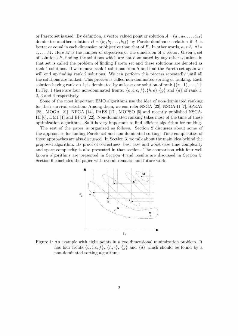
or Pareto set is used. By definition, a vector valued point or solution A = (a1, a2, . . . , aM)dominates another solution B = (b1, b2, . . . , bM) by Pareto-dominance relation if A isbetter or equal in each dimension or objective than that of B. In other words, ai ⪰ bi ∀i =1, . . . ,M . Here M is the number of objectives or the dimension of a vector. Given a setof solutions P , finding the solutions which are not dominated by any other solutions inthat set is called the problem of finding Pareto set and these solutions are denoted asrank 1 solutions. If we remove rank 1 solutions from S and find the Pareto set again wewill end up finding rank 2 solutions. We can perform this process repeatedly until allthe solutions are ranked. This process is called non-dominated sorting or ranking. Eachsolution having rank r > 1, is dominated by at least one solution of rank {(r−1), . . . ,1}.In Fig. 1 there are four non-dominated fronts: {a, b, c, f},{h, e},{g} and {d} of rank 1,2, 3 and 4 respectively.

Some of the most important EMO algorithms use the idea of non-dominated rankingfor their survival selection. Among them, we can refer NSGA [23], NSGA-II [7], SPEA2[28], MOGA [21], NPGA [14], PAES [17], MOPSO [5] and recently published NSGA-III [6], DM1 [1] and EPCS [22]. Non-dominated ranking takes most of the time of theseoptimization algorithms. So it is very important to find efficient algorithm for ranking.

The rest of the paper is organized as follows. Section 2 discusses about some ofthe approaches for finding Pareto set and non-dominated sorting. Time complexities ofthose approaches are also discussed. In Section 3, we talk about the main idea behind theproposed algorithm. Its proof of correctness, best case and worst case time complexityand space complexity is also presented in that section. The comparison with four wellknown algorithms are presented in Section 4 and results are discussed in Section 5.Section 6 concludes the paper with overall remarks and future work.

f1

a

b

h

e

f2

g

d

c

f

Figure 1: An example with eight points in a two dimensional minimization problem. Ithas four fronts {a, b, c, f}, {h, e}, {g} and {d} which should be found by anon-dominated sorting algorithm.

2

2 RELATED WORK

The methods for finding Pareto set and non-dominated sorting can be divided into twocategories– sequential and divide-and-conquer approach. Given a set of vectors, sequen-tial brute force method for finding the Pareto set is to compare each solution to everyother solution to check whether they dominate each other. If either of them is domi-nated, then that is removed from current set. It can be used to find the non-dominatedranking by repeating the process and removing the ranked solutions or points from theset [23]. The algorithm has O(MN3) complexity because of repeated comparisons. Dueto high computational complexity of [23], Deb et al. [7] described a computationallyfaster version, termed fast non-dominated sort, whose complexity is O(MN2). It usesthe fact that pairwise comparisons can be saved and used later to find the rank of solu-tions other than the Pareto set. However, space complexity is O(N2) because it savespairwise comparisons.

McClymont and Keedwell [19] described a set of algorithms which improves spacecomplexity to O(N) and has time complexity Ø(MN2). Among them deductive sort isreported to work best. The algorithm consists of multiple passes and one pass is com-pleted by removing dominated solutions with an arbitrary unranked solution. Cornersort [25] is a new approach for finding non-dominated ranking of vectors which workssimilar to deductive sort. But instead of choosing an arbitrary vector for checking dom-inance, it always chooses a vector which is guaranteed to be in current rank. So itworks better than deductive sort in some cases but has the same worst case complex-ity. Recently, an efficient approach of non-dominated ranking called ENS [27] has beendescribed. This method uses the idea of sorting the solutions by the values of first objec-tive with in-place heap sort. In case of tie, the authors use lexicographic ordering. Thisalgorithm can achieve best case complexity O(MN logN) although it has O(MN2) inworst cases. Other methods e.g. dominance tree based non-dominated sorting [10], non-dominated rank sort or omni-optimizer [9] and arena’s principle [24] can also be usedto improve the best case time complexity upto O(MN

√N). However, the worst case

time complexity remains the same as O(MN2). Recently, parallel GPU based NSGA-IIalgorithm [13] has been proposed to speed up the non-dominated sorting and other stepsof the evolutionary algorithm.

Unlike the sequential algorithms, the set of divide-and-conquer algorithms work byrepeatedly dividing the data using objective values. These methods are asymptoticallyfaster than sequential ones in the worst case for fixed number of objectives. The firstdivide-and-conquer method was proposed by Kung et al. [18] for finding the Paretoset. This method is later analyzed by Bentley [2]. This algorithm divides the dataand reduces dimensions recursively. At first, it divides input set into two halves by themedian of their first objective values. If size of the set is still more than one and if thereis unused dimension left, then the set is divided again with unused dimension. Thedivision goes on until data can no longer be divided or unused dimensions are reducedto two. When the dimension becomes less than 3, special-case algorithm is appliedfor ranking which has complexity O(N logN). If the dimension is not fixed then itscomplexity is bounded by O(MN2) [4,20]. These algorithms exhibit many unnecessary

3

comparisons which increases with the number of objectives [12]. The space complexityis said to be O(N) for Kung’s algorithm. Bentley [3] improved the average case of thisdivide-and-conquer algorithm. It assumes the fact that size of Pareto set of vectors isequal to O(logM−1N) on average. One can find the non-dominated ranking by repeatingKung’s algorithm the number of times equal to number of ranks which gives complexityO(N2 logM−2N). By removing the repeated comparisons, Jensen [16] and Yukish [26]both extended Kung’s algorithm to find the Pareto set of vectors and perform non-dominated ranking in time O(N logM−1N). Jensen’s algorithm assumes that, for anyobjective, no two vectors have the same objective value [10]. Because of this assumptionit generates different Pareto ranking from the baseline algorithm of NSGA-II [7]. It wascorrected later in [4, 11]. Buzdalov et al. proved the time complexity of non-dominatedranking to be O(N logM−1N) for fixed dimension. Our aim is to find better algorithmsin terms of N and M both.

3 PROPOSED METHOD

3.1 Basic Idea

In this section we propose an algorithm named best order sort (BOS) which reduces thenumber of comparisons in the worst case. The main idea of the algorithm is described inFig. 2. For each solution s, we can get a set for each objective that denotes the solutionswhich are not worse than s in that objective. So there will be M sets as there are Mobjectives. To find the rank of s, only one set T is sufficient to be considered. Somemembers t ∈ T of the set dominate s while others are non-dominated with s. Supposehighest rank of T is r. The rank of s will then be (r + 1). Although any of the M setscan be considered to find rank of s, our method finds the smallest set by sorting thepopulation with their objective values.

s1

m=1 m=2 m=M

s2

sN

Figure 2: The basic idea of the proposed method is that there are M sets for eachsolution which denote the ‘not-worse’ solutions in corresponding objective.The algorithm finds the smallest set to compare and finds their ranks.

4

3.2 The Algorithm

The algorithm starts with initializing N ×M empty sets denoted by Lji (see Algorithm

1). Here N is the size of population and M is the number of objectives. Lrj denotes the

set of solutions which has rank r and they are found in j-th objective. The algorithmsaves sorted population in Qj which denotes that j-th objective value is used for sorting.It maintains a objective list Cu = {1,2, . . . ,M} for each solution u. It signifies that, ifwe want to check whether a solution s is dominated by u then only the objectives in Cu

needs to be compared. The variable isRanked(s) = false denotes that solution s is notranked yet. We initialize number of solutions done SC to zero, ranks of solutions R(s)equal to zero for all s ∈ P and fronts found so far RC = 1.

At first, we sort the solutions according to each objective j and put those into sortedlist Qj (see line 8 of Algorithm 1). We use lexicographic order if two objective valuesare same. In that case, if the first objective values are same then sorting will be basedon the second objective value. Note that we just need to perform single lexicographicordering for the first objective. We can then use the information of first objective to findlexicographic order of other objectives.

Algorithm 1: Initialization

Data: Population P of size N and objective MResult: Sorted set of solutions in Qj

1 Lij ← ∅, ∀ j = 1,2, . . . ,M, ∀ i = 1,2, . . . ,N// global variable

2 Ci ← {1,2, . . . ,M} ∀ i = 1,2, . . . ,N// comparison set, global variable

3 isRanked(P )← false// solutions ranked or not, global variable

4 SC ← 0// number of solutions already ranked, global variable

5 RC ← 1// number of fronts discovered so far, global variable

6 R(P )← 0// Rank of solutions, global variable

7 for j = 1 to M do8 Qj ← Sort P by j-th objective value, use lexicographic order in case of tie;

// lexicographic sort

9 end

Algorithm 2 describes the main procedure for finding the non-dominated ranking. Ittakes the lexicographically sorted population Qj for each objective j. The algorithmstarts taking the first element s from the sorted list Q1 of first objective, which can bedenoted by Q1(1). Then it excludes objective {1} from the list Cs. This is because, ifother solution t is compared with s later, t is already dominated in objective 1. Next,the algorithm checks whether s is already ranked or not. If it is ranked then it will be

included to the corresponding list LR(s)1 . For instance, if s has to be included in L5

2,then s’s rank is 5 and it is found in second objective. Lj is the set of all solutions that isneeded to find rank of s (see Algorithm 3) because they are not worse than s in objectivej. At the end of this algorithm, each solution should appear in every objective set Lj

only once, if line 14 of Algorithm 2 is not executed.

5

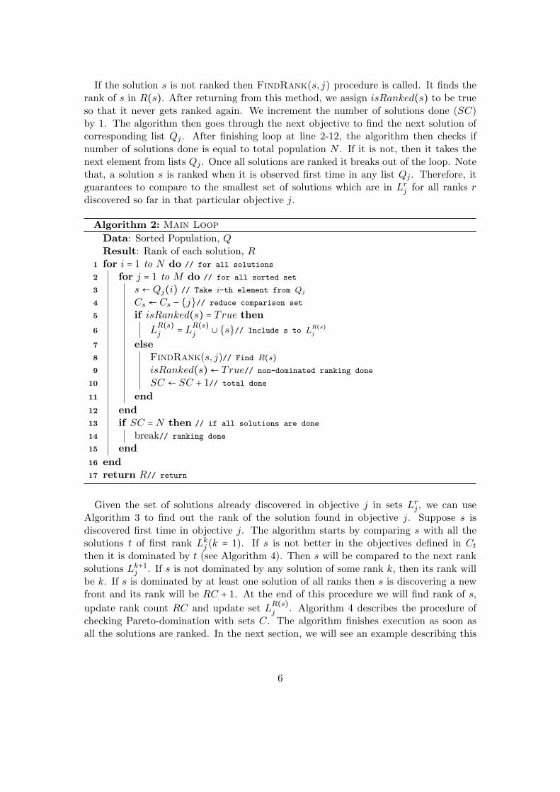
If the solution s is not ranked then FindRank(s, j) procedure is called. It finds therank of s in R(s). After returning from this method, we assign isRanked(s) to be trueso that it never gets ranked again. We increment the number of solutions done (SC)by 1. The algorithm then goes through the next objective to find the next solution ofcorresponding list Qj . After finishing loop at line 2-12, the algorithm then checks ifnumber of solutions done is equal to total population N . If it is not, then it takes thenext element from lists Qj . Once all solutions are ranked it breaks out of the loop. Notethat, a solution s is ranked when it is observed first time in any list Qj . Therefore, itguarantees to compare to the smallest set of solutions which are in Lr

j for all ranks rdiscovered so far in that particular objective j.

Algorithm 2: Main Loop

Data: Sorted Population, QResult: Rank of each solution, R

1 for i = 1 to N do // for all solutions

2 for j = 1 to M do // for all sorted set

3 s← Qj(i) // Take i-th element from Qj

4 Cs ← Cs − {j}// reduce comparison set

5 if isRanked(s) = True then

6 LR(s)j = L

R(s)j ∪ {s}// Include s to L

R(s)j

7 else8 FindRank(s, j)// Find R(s)9 isRanked(s)← True// non-dominated ranking done

10 SC ← SC + 1// total done

11 end

12 end13 if SC = N then // if all solutions are done

14 break// ranking done

15 end

16 end17 return R// return

Given the set of solutions already discovered in objective j in sets Lrj , we can use

Algorithm 3 to find out the rank of the solution found in objective j. Suppose s isdiscovered first time in objective j. The algorithm starts by comparing s with all thesolutions t of first rank Lk

j (k = 1). If s is not better in the objectives defined in Ct

then it is dominated by t (see Algorithm 4). Then s will be compared to the next ranksolutions Lk+1

j . If s is not dominated by any solution of some rank k, then its rank willbe k. If s is dominated by at least one solution of all ranks then s is discovering a newfront and its rank will be RC + 1. At the end of this procedure we will find rank of s,

update rank count RC and update set LR(s)j . Algorithm 4 describes the procedure of

checking Pareto-domination with sets C. The algorithm finishes execution as soon asall the solutions are ranked. In the next section, we will see an example describing this

6

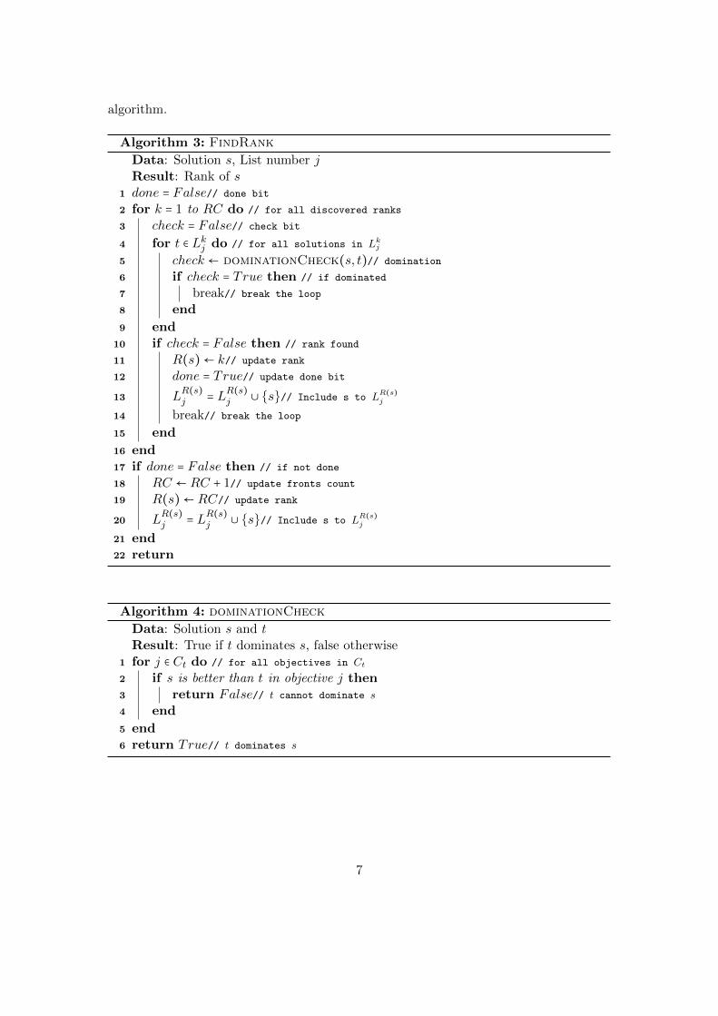
algorithm.

Algorithm 3: FindRank

Data: Solution s, List number jResult: Rank of s

1 done = False// done bit

2 for k = 1 to RC do // for all discovered ranks

3 check = False// check bit

4 for t ∈ Lkj do // for all solutions in Lk

j

5 check ← dominationCheck(s, t)// domination

6 if check = True then // if dominated

7 break// break the loop

8 end

9 end10 if check = False then // rank found

11 R(s)← k// update rank

12 done = True// update done bit

13 LR(s)j = L

R(s)j ∪ {s}// Include s to L

R(s)j

14 break// break the loop

15 end

16 end17 if done = False then // if not done

18 RC ← RC + 1// update fronts count

19 R(s)← RC// update rank

20 LR(s)j = L

R(s)j ∪ {s}// Include s to L

R(s)j

21 end22 return

Algorithm 4: dominationCheck

Data: Solution s and tResult: True if t dominates s, false otherwise

1 for j ∈ Ct do // for all objectives in Ct

2 if s is better than t in objective j then3 return False// t cannot dominate s

4 end

5 end6 return True// t dominates s

7

3.3 Illustrative Example

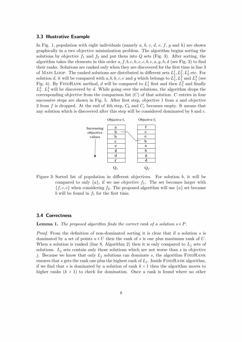
In Fig. 1, population with eight individuals (namely a, b, c, d, e, f , g and h) are showngraphically in a two objective minimization problem. The algorithm begins sorting thesolutions by objective f1 and f2 and put them into Q sets (Fig. 3). After sorting, thealgorithm takes the elements in this order a, f, b, c, h, e, c, b, e, a, g, h, d (see Fig. 3) to findtheir ranks. Solutions are ranked only when they are discovered for the first time in line 3of Main Loop. The ranked solutions are distributed in different sets L1

1, L21, L

12 etc. For

solution d, it will be compared with a, b, h, c, e and g which belongs to L11, L

21 and L3

1 (seeFig. 4). By FindRank method, d will be compared to L1

1 first and then L21 and finally

L31. L4

1 will be discovered by d. While going over the solutions, the algorithm drops thecorresponding objective from the comparison list (C) of that solution. C entries in foursuccessive steps are shown in Fig. 5. After first step, objective 1 from a and objective2 from f is dropped. At the end of 4th step, Cb and Cc becomes empty. It means thatany solution which is discovered after this step will be considered dominated by b and c.

Q1

a

b

h

c

e

g

d

d

f

c

e

ba

h

g

Increasing

objective

values

Objective f1

f

Objective f2

Q2

Figure 3: Sorted list of population in different objectives. For solution b, it will becompared to only {a}, if we use objective f1. The set becomes larger with{f, c, e} when considering f2. The proposed algorithm will use {a} set becauseb will be found in f1 for the first time.

3.4 Correctness

Lemma 1. The proposed algorithm finds the correct rank of a solution s ∈ P .

Proof. From the definition of non-dominated sorting it is clear that if a solution s isdominated by a set of points u ∈ U then the rank of s is one plus maximum rank of U .When a solution is ranked (line 8, Algorithm 2) then it is only compared to Lj sets ofsolutions. Lj sets contain only those solutions which are not worse than s in objectivej. Because we know that only Lj solutions can dominate s, the algorithm FindRankensures that s gets the rank one plus the highest rank of Lj . Inside FindRank algorithm,if we find that s is dominated by a solution of rank k = 1 then the algorithm moves tohigher ranks (k > 1) to check for domination. Once a rank is found where no other

8

Obj f1: L1 sets a, b, c g

Front 1 Front 2 Front 3

Obj f2: L2 sets f, c, b, a

h, e

e, h

3 4

4

d

g

Figure 4: Four different fronts are discovered by the algorithm which are again dis-tributed in four different fronts. Rank 1 solutions are given by union of L1

1

and L12 sets etc. The algorithm exits as soon as all the solutions are ranked,

otherwise it would have been true that L11 = L1

2, L21 = L2

2 and so on.

{1, 2}Ca:

Cb:

Cc:

Cd:

Ce:

Cf:

Cg:

Ch:

{1, 2}

{1, 2}

{1, 2}

{1, 2}

{1, 2}

{1, 2}

{1, 2}

{2}Ca:

Cb:

Cc:

Cd:

Ce:

Cf:

Cg:

Ch:

{1, 2}

{1,2}

{1, 2}

{1, 2}

{1}

{1, 2}

{1, 2}

{2}Ca:

Cb:

Cc:

Cd:

Ce:

Cf:

Cg:

Ch:

{2}

{1}

{1, 2}

{1, 2}

{1}

{1, 2}

{1, 2}

{2}Ca:

Cb:

Cc:

Cd:

Ce:

Cf:

Cg:

Ch:

{2}

{1}

{1, 2}

{1}

{1}

{1, 2}

{2}

{2}Ca:

Cb:

Cc:

Cd:

Ce:

Cf:

Cg:

Ch:

{}

{}

{1, 2}

{1}

{1}

{1, 2}

{2}

Figure 5: Four steps execution of the loop at line 1 in Algorithm 2 is shown. Droppingsome objectives from the list indicates that a solution discovered later is alreadydominated on those objectives.

solution of that rank dominates s, the correct rank of s is identified as the same rankas of those. If s is found to be dominated by at least one solution of each rank foundso far, a new rank (RC + 1) is introduced with the solution s. In each case, comparingsolutions of s have smaller set of objectives to compare. The objectives in which s isalready dominated, are dropped from the objective list. Therefore each comparison iscorrect. Thus each solution finds its rank correctly.

3.5 Best Case Complexity

Best case for this algorithm happens when the population has N fronts, each front havingonly one solution. In this case, we will get the similar order in all Qj after sorting byAlgorithm 1. While executing line 2 of Algorithm 2 with j = 1 up to j = M , all theobjectives will be deleted (see line 4) from the objective list Cs. So there will be noobjective value comparison. Total execution time for line 1 and 2 of Algorithm 2 isO(MN). Therefore we get the best case time complexity O(MN logN).

9

3.6 Average Case Time and Space Complexity

Theorem 1. Under independence assumption, in average case, best order sort has timecomplexity is O(MN logN +MN2) . Its space complexity is O(MN).

First we assume that solutions are independently distributed along the objectives.The assumption is given below.

Definition 3.1 (Independence Assumption). Distribution of one objective values of thepopulation is statistically independent of the distribution of other objective values.

Proof. Average case complexity depends on number of solutions to compare and totalnumber of objectives in objective lists C. We will do amortized analysis here. A solutionis ranked when it is found first time in Algorithm 2 (line 3). In one row (row is found byline 2, for same i and all j = {1,2, . . . ,M}), only unique solutions, those previously notfound, are ranked by Algorithm 3. Suppose, on average, p unique solutions are foundin one row. As the size of M grows, there will be increase of unique solutions accordingto independence assumption. So p is a function of M i.e. p = F (M). In each row, Mobjectives will be deleted. Deletion is done in O(1) time with the help of M ×N directaccess pointers to the members of the lists. Suppose r denotes the row number (value ofi) when Algorithm 2 terminates first loop (line 1) and breaks out of the loop at line 14.It means that, all the solutions are already discovered (appears first time) by row r fromthe sorted lists Qj , j ∈ {1,2, . . . ,M}. In this case, pr = N is a constraint that needs tobe maintained. As we have seen from the algorithm, solution s is only compared to allthe solutions found in that objective previously, s will be compared to (r − 1) solutionsif it is found in row r. Total remaining objectives for p solutions will be (Mp−M) afterexecuting one row. So number of objective value comparisons is ((Mp−M)/p)× (r−1).It should be multiplied by p as we will compare p solutions in a row. Total number ofcomparisons can be found if we execute the algorithm up to r row where r = N/p.

T (M,N) = (Mp −M)r=N/p

∑r=1

(r − 1)

= O(Mp) ×O (N2

p2) = O(MN2/p)

The equation holds for 2 ≤ p ≤ M and p is an integer. This is because if p = 1, thenall the objectives in the list will be deleted per each row and best case of the algorithmis achieved. For p =

√M we get the complexity O(N2

√M). Worst case is achieved

when p = 2. Then only two solutions are found in each row (Fig. 6) and r = N/2. Thecomplexity becomes O(MN2) where independence assumption is violated. When p is alinear function of M then we achieve complexity O(N2) for ranking. If the Algorithm2 finds unique solution each time line 3 is executed, then p = M and r = N/M . Thecomplexity becomes O(N2). Lexicographical sort (Algorithm 1) takes O(MN logN)time. So the time complexity of this algorithm is O (MN logN +MN2) under inde-pendence assumption. If M number of processors are used for lexicographic sort, then

10

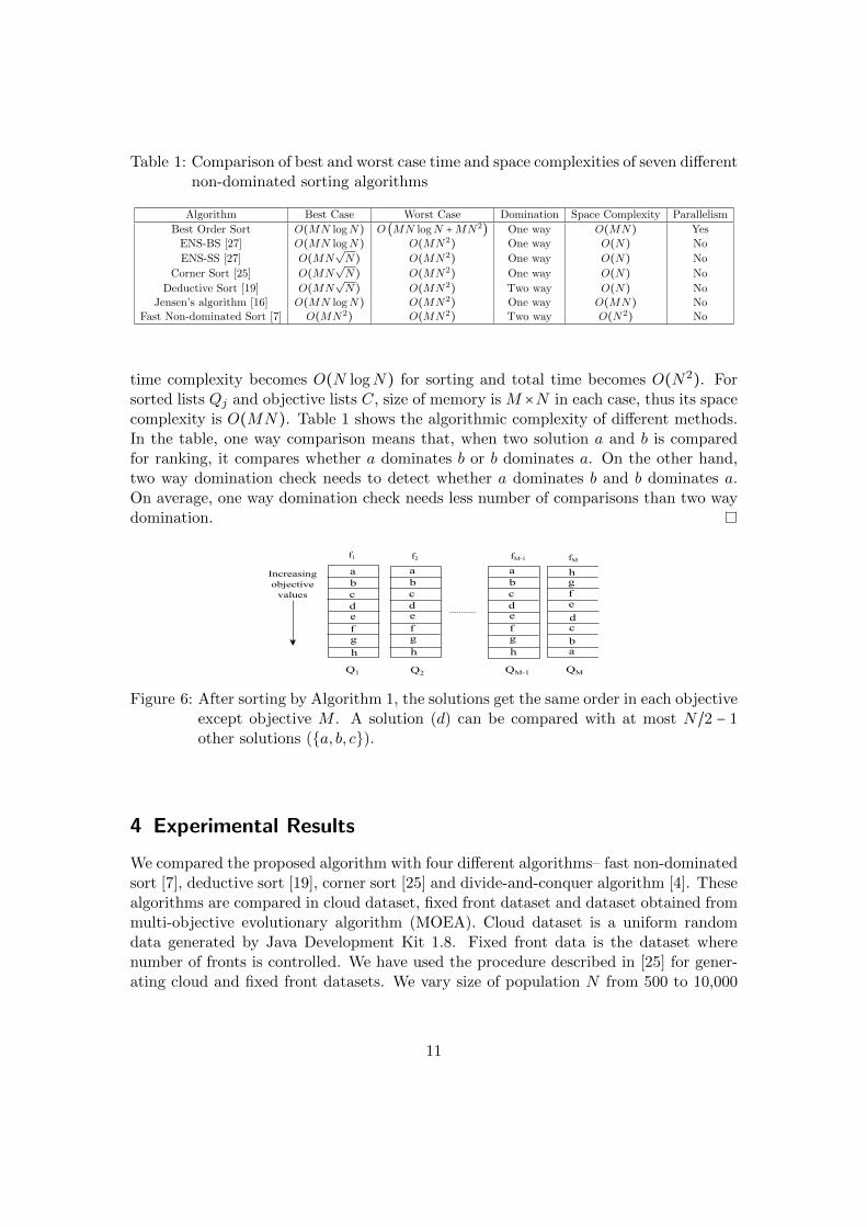
Table 1: Comparison of best and worst case time and space complexities of seven differentnon-dominated sorting algorithms

Algorithm Best Case Worst Case Domination Space Complexity Parallelism

Best Order Sort O(MN logN) O (MN logN +MN2) One way O(MN) Yes

ENS-BS [27] O(MN logN) O(MN2) One way O(N) No

ENS-SS [27] O(MN√N) O(MN2) One way O(N) No

Corner Sort [25] O(MN√N) O(MN2) One way O(N) No

Deductive Sort [19] O(MN√N) O(MN2) Two way O(N) No

Jensen’s algorithm [16] O(MN logN) O(MN2) One way O(MN) NoFast Non-dominated Sort [7] O(MN2) O(MN2) Two way O(N2) No

time complexity becomes O(N logN) for sorting and total time becomes O(N2). Forsorted lists Qj and objective lists C, size of memory is M ×N in each case, thus its spacecomplexity is O(MN). Table 1 shows the algorithmic complexity of different methods.In the table, one way comparison means that, when two solution a and b is comparedfor ranking, it compares whether a dominates b or b dominates a. On the other hand,two way domination check needs to detect whether a dominates b and b dominates a.On average, one way domination check needs less number of comparisons than two waydomination.

Q1

a

d

f

c

e

b

h

g

Increasing

objective

values

f1

Q2

a

d

f

c

e

b

h

g

a

d

f

c

e

b

h

g

hg

fe

dc

ba

QM-1 QM

f2 fM-1 fM

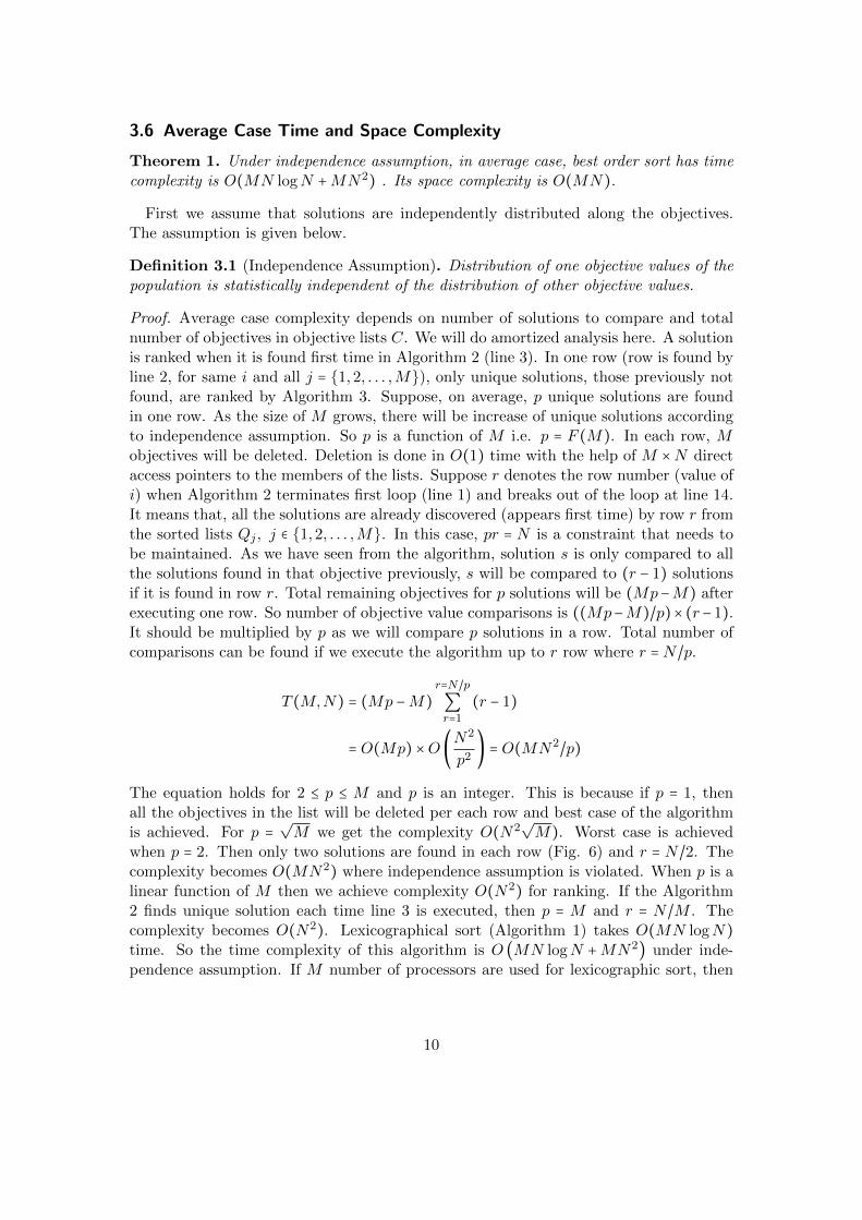
Figure 6: After sorting by Algorithm 1, the solutions get the same order in each objectiveexcept objective M . A solution (d) can be compared with at most N/2 − 1other solutions ({a, b, c}).

4 Experimental Results

We compared the proposed algorithm with four different algorithms– fast non-dominatedsort [7], deductive sort [19], corner sort [25] and divide-and-conquer algorithm [4]. Thesealgorithms are compared in cloud dataset, fixed front dataset and dataset obtained frommulti-objective evolutionary algorithm (MOEA). Cloud dataset is a uniform randomdata generated by Java Development Kit 1.8. Fixed front data is the dataset wherenumber of fronts is controlled. We have used the procedure described in [25] for gener-ating cloud and fixed front datasets. We vary size of population N from 500 to 10,000

11

0 5 10 15 200

5

10

15x 10

9

Number of Objectives

Num

ber

of C

ompa

rison

s

fnsdscorddcbos

(a) Comparison

0 5 10 15 200

2

4

6

8

10x 10

4

Number of Objectives

Tot

al R

untim

e (m

s)

fnsdscorddcbos

(b) Time

Figure 7: Number of comparisons and runtime (in milliseconds) for cloud dataset of size10,000 for increasing number of objectives. Results for fast non-dominatedsort (fns), deductive sort (ds), corner sort (cor), divide-and-corner sort (ddc)and best order sort (bos) is shown.

with an increment of 500 in cloud dataset. In another test (Fig. 6), number of objectivesare varied from 2 to 20 to evaluate performance with population size 10,000. For fixedfront dataset, number of front is varied from 1 to 10 where number of solution is kept10,000 with objectives 5, 10, 15 and 20. MOEA dataset is obtained by running 200generations of NSGA-II algorithm in DTLZ1 and DTLZ2 [8], WFG1 and WFG2 [15]problems with 5, 10, 15 and 20 objectives. In these cases, all the parameter valuesare kept as standard ones. For example, simulated binary crossover with polynomialmutation are employed with probabilities 0.80 and (1/number of variables) respectively.Each algorithm is repeated 30 times in 30 different datasets to get the averages. All thealgorithms are optimized and implemented in Java Development Kit 1.8 update 65 andrun in Dell computer with 3.2 GHz Intel core i7 and 64 bit Windows 7 machine.

5 Discussion

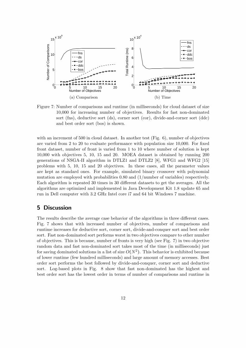
The results describe the average case behavior of the algorithms in three different cases.Fig. 7 shows that with increased number of objectives, number of comparisons andruntime increases for deductive sort, corner sort, divide-and-conquer sort and best ordersort. Fast non-dominated sort performs worst in two objectives compare to other numberof objectives. This is because, number of fronts is very high (see Fig. 7) in two objectiverandom data and fast non-dominated sort takes most of the time (in milliseconds) justfor saving dominated solutions in a list of size O(N2). This behavior is exhibited becauseof lower runtime (few hundred milliseconds) and large amount of memory accesses. Bestorder sort performs the best followed by divide-and-conquer, corner sort and deductivesort. Log-based plots in Fig. 8 show that fast non-dominated has the highest andbest order sort has the lowest order in terms of number of comparisons and runtime in

12

103

104

105

1010

Number of Soutions

Num

ber

of C

ompa

rison

s

fnsdscorddcbos

(a) M = 5

103

104

105

1010

Number of Soutions

Num

ber

of C

ompa

rison

s

fnsdscorddcbos

(b) M = 10

103

104

105

1010

Number of Soutions

Num

ber

of C

ompa

rison

s

fnsdscorddcbos

(c) M = 15

103

104

105

1010

Number of Soutions

Num

ber

of C

ompa

rison

s

fnsdscorddcbos

(d) M = 20

103

104

102

104

Number of Soutions

Tot

al R

untim

e (m

s)

fnsdscorddcbos

(e) M = 5

103

104

101

102

103

104

105

Number of Soutions

Tot

al R

untim

e (m

s)

fnsdscorddcbos

(f) M = 10

103

104

102

104

Number of Soutions

Tot

al R

untim

e (m

s)

fnsdscorddcbos

(g) M = 15

103

104

102

104

Number of Soutions

Tot

al R

untim

e (m

s)

fnsdscorddcbos

(h) M = 20

Figure 8: Figure describes number of comparisons and runtime (in milliseconds) withincreasing population size for cloud dataset in objectives 5, 10, 15 and 20.Results for fast non-dominated sort (fns), deductive sort (ds), corner sort (cor),divide-and-conquer sort (ddc) and best order sort (bos) is shown.

0 2 4 6 8 100

5

10

15x 10

9

Number of Fronts

Num

ber

of C

ompa

rison

s

fnsdscorddcbos

(a) M = 5

0 2 4 6 8 100

0.5

1

1.5

2x 10

10

Number of Fronts

Num

ber

of C

ompa

rison

s

fnsdscorddcbos

(b) M = 10

0 2 4 6 8 100

0.5

1

1.5

2x 10

10

Number of Fronts

Num

ber

of C

ompa

rison

s

fnsdscorddcbos

(c) M = 15

0 2 4 6 8 100

0.5

1

1.5

2

2.5x 10

10

Number of Fronts

Num

ber

of C

ompa

rison

s

fnsdscorddcbos

(d) M = 20

0 2 4 6 8 100

1

2

3

4

5x 10

4

Number of Fronts

Tot

al R

untim

e (m

s)

fnsdscorddcbos

(e) M = 5

0 2 4 6 8 100

1

2

3

4

5x 10

4

Number of Fronts

Tot

al R

untim

e (m

s)

fnsdscorddcbos

(f) M = 10

0 2 4 6 8 100

1

2

3

4

5x 10

4

Number of Fronts

Tot

al R

untim

e (m

s)

fnsdscorddcbos

(g) M = 15

0 2 4 6 8 100

1

2

3

4

5x 10

4

Number of Fronts

Tot

al R

untim

e (m

s)

fnsdscorddcbos

(h) M = 20

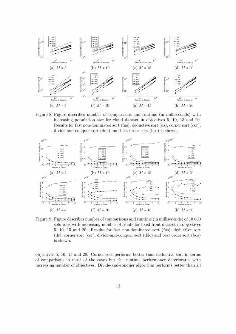
Figure 9: Figure describes number of comparisons and runtime (in milliseconds) of 10,000solutions with increasing number of fronts for fixed front dataset in objectives5, 10, 15 and 20. Results for fast non-dominated sort (fns), deductive sort(ds), corner sort (cor), divide-and-conquer sort (ddc) and best order sort (bos)is shown.

objectives 5, 10, 15 and 20. Corner sort performs better than deductive sort in termsof comparisons in most of the cases but the runtime performance deteriorates withincreasing number of objectives. Divide-and-conquer algorithm performs better than all

13

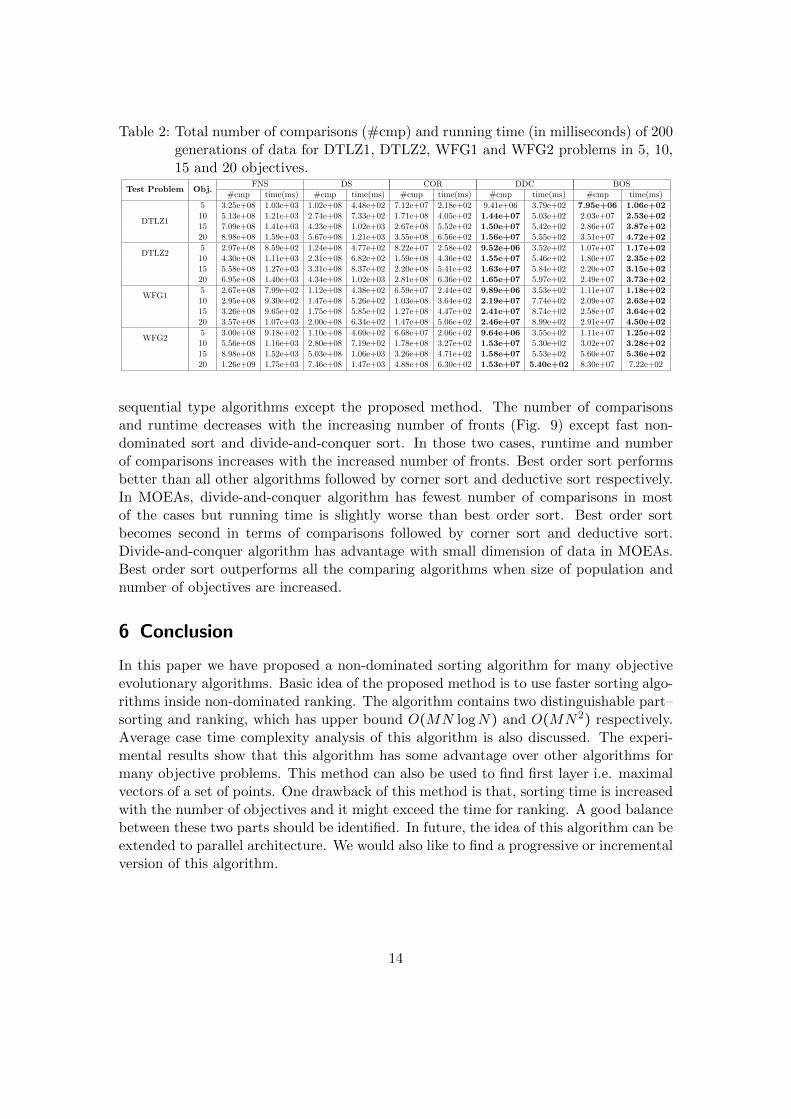
Table 2: Total number of comparisons (#cmp) and running time (in milliseconds) of 200generations of data for DTLZ1, DTLZ2, WFG1 and WFG2 problems in 5, 10,15 and 20 objectives.

Test Problem Obj.FNS DS COR DDC BOS

#cmp time(ms) #cmp time(ms) #cmp time(ms) #cmp time(ms) #cmp time(ms)

DTLZ1

5 3.25e+08 1.03e+03 1.02e+08 4.48e+02 7.12e+07 2.18e+02 9.41e+06 3.79e+02 7.95e+06 1.06e+0210 5.13e+08 1.21e+03 2.74e+08 7.33e+02 1.71e+08 4.05e+02 1.44e+07 5.03e+02 2.03e+07 2.53e+0215 7.09e+08 1.41e+03 4.23e+08 1.02e+03 2.67e+08 5.52e+02 1.50e+07 5.42e+02 2.86e+07 3.87e+0220 8.98e+08 1.59e+03 5.67e+08 1.21e+03 3.55e+08 6.56e+02 1.56e+07 5.55e+02 3.51e+07 4.72e+02

DTLZ25 2.97e+08 8.59e+02 1.24e+08 4.77e+02 8.22e+07 2.58e+02 9.52e+06 3.52e+02 1.07e+07 1.17e+0210 4.30e+08 1.11e+03 2.31e+08 6.82e+02 1.59e+08 4.36e+02 1.55e+07 5.46e+02 1.80e+07 2.35e+0215 5.58e+08 1.27e+03 3.31e+08 8.37e+02 2.20e+08 5.41e+02 1.63e+07 5.84e+02 2.20e+07 3.15e+0220 6.95e+08 1.40e+03 4.34e+08 1.02e+03 2.81e+08 6.36e+02 1.65e+07 5.97e+02 2.49e+07 3.73e+02

WFG15 2.67e+08 7.99e+02 1.12e+08 4.38e+02 6.59e+07 2.44e+02 9.89e+06 3.53e+02 1.11e+07 1.18e+0210 2.95e+08 9.30e+02 1.47e+08 5.26e+02 1.03e+08 3.64e+02 2.19e+07 7.74e+02 2.09e+07 2.63e+0215 3.26e+08 9.65e+02 1.75e+08 5.85e+02 1.27e+08 4.47e+02 2.41e+07 8.74e+02 2.58e+07 3.64e+0220 3.57e+08 1.07e+03 2.00e+08 6.34e+02 1.47e+08 5.06e+02 2.46e+07 8.99e+02 2.91e+07 4.50e+02

WFG25 3.00e+08 9.18e+02 1.10e+08 4.69e+02 6.68e+07 2.06e+02 9.64e+06 3.55e+02 1.11e+07 1.25e+0210 5.56e+08 1.16e+03 2.80e+08 7.19e+02 1.78e+08 3.27e+02 1.53e+07 5.30e+02 3.02e+07 3.28e+0215 8.98e+08 1.52e+03 5.03e+08 1.06e+03 3.26e+08 4.71e+02 1.58e+07 5.53e+02 5.60e+07 5.36e+0220 1.26e+09 1.75e+03 7.46e+08 1.47e+03 4.88e+08 6.30e+02 1.53e+07 5.40e+02 8.30e+07 7.22e+02

sequential type algorithms except the proposed method. The number of comparisonsand runtime decreases with the increasing number of fronts (Fig. 9) except fast non-dominated sort and divide-and-conquer sort. In those two cases, runtime and numberof comparisons increases with the increased number of fronts. Best order sort performsbetter than all other algorithms followed by corner sort and deductive sort respectively.In MOEAs, divide-and-conquer algorithm has fewest number of comparisons in mostof the cases but running time is slightly worse than best order sort. Best order sortbecomes second in terms of comparisons followed by corner sort and deductive sort.Divide-and-conquer algorithm has advantage with small dimension of data in MOEAs.Best order sort outperforms all the comparing algorithms when size of population andnumber of objectives are increased.

6 Conclusion

In this paper we have proposed a non-dominated sorting algorithm for many objectiveevolutionary algorithms. Basic idea of the proposed method is to use faster sorting algo-rithms inside non-dominated ranking. The algorithm contains two distinguishable part–sorting and ranking, which has upper bound O(MN logN) and O(MN2) respectively.Average case time complexity analysis of this algorithm is also discussed. The experi-mental results show that this algorithm has some advantage over other algorithms formany objective problems. This method can also be used to find first layer i.e. maximalvectors of a set of points. One drawback of this method is that, sorting time is increasedwith the number of objectives and it might exceed the time for ranking. A good balancebetween these two parts should be identified. In future, the idea of this algorithm can beextended to parallel architecture. We would also like to find a progressive or incrementalversion of this algorithm.

14

Acknowledgment

This material is based in part upon work supported by the National Science Foundationunder Cooperative Agreement No. DBI-0939454. Any opinions, findings, and conclu-sions or recommendations expressed in this material are those of the author(s) and donot necessarily reflect the views of the National Science Foundation.

References

[1] S. Adra and P. Fleming. Diversity management in evolutionary many-objectiveoptimization. Evolutionary Computation, IEEE Transactions on, 15(2):183–195,April 2011.

[2] J. L. Bentley. Multidimensional divide-and-conquer. Commun. ACM, 23(4):214–229, Apr. 1980.

[3] J. L. Bentley, H. T. Kung, M. Schkolnick, and C. D. Thompson. On the averagenumber of maxima in a set of vectors and applications. J. ACM, 25(4):536–543,Oct. 1978.

[4] M. Buzdalov and A. Shalyto. A provably asymptotically fast version of the general-ized Jensen algorithm for non-dominated sorting. In T. Bartz-Beielstein, J. Branke,B. Filipic, and J. Smith, editors, Parallel Problem Solving from Nature - PPSNXIII, volume 8672 of Lecture Notes in Computer Science, pages 528–537. SpringerInternational Publishing, 2014.

[5] C. A. Coello Coello and M. Lechuga. MOPSO: a proposal for multiple objectiveparticle swarm optimization. In Evolutionary Computation, 2002. CEC ’02. Pro-ceedings of the 2002 Congress on, volume 2, pages 1051–1056, 2002.

[6] K. Deb and H. Jain. An evolutionary many-objective optimization algorithm usingreference-point-based nondominated sorting approach, part I: Solving problems withbox constraints. Evolutionary Computation, IEEE Transactions on, 18(4):577–601,Aug 2014.

[7] K. Deb, A. Pratap, S. Agarwal, and T. Meyarivan. A fast and elitist multiobjectivegenetic algorithm: Nsga-II. Evolutionary Computation, IEEE Transactions on,6(2):182–197, Apr 2002.

[8] K. Deb, L. Thiele, M. Laumanns, and E. Zitzler. Scalable multi-objective optimiza-tion test problems. In Evolutionary Computation, 2002. CEC ’02. Proceedings ofthe 2002 Congress on, volume 1, pages 825–830, May 2002.

[9] K. Deb and S. Tiwari. Omni-optimizer: A procedure for single and multi-objectiveoptimization. In Proceedings of the Third International Conference on Evolution-ary Multi-Criterion Optimization, EMO’05, pages 47–61, Berlin, Heidelberg, 2005.Springer-Verlag.

15

[10] H. Fang, Q. Wang, Y.-C. Tu, and M. F. Horstemeyer. An efficient non-dominatedsorting method for evolutionary algorithms. Evol. Comput., 16(3):355–384, Sept.2008.

[11] F.-A. Fortin, S. Grenier, and M. Parizeau. Generalizing the improved run-timecomplexity algorithm for non-dominated sorting. In Proceedings of the 15th AnnualConference on Genetic and Evolutionary Computation, GECCO ’13, pages 615–622,New York, NY, USA, 2013. ACM.

[12] P. Godfrey, R. Shipley, and J. Gryz. Maximal vector computation in large datasets. In Proceedings of the 31st International Conference on Very Large Data Bases,VLDB ’05, pages 229–240. VLDB Endowment, 2005.

[13] S. Gupta and G. Tan. A scalable parallel implementation of evolutionary algorithmsfor multi-objective optimization on gpus. In Evolutionary Computation (CEC),2015 IEEE Congress on, pages 1567–1574, May 2015.

[14] J. Horn, N. Nafpliotis, and D. Goldberg. A niched Pareto genetic algorithm formultiobjective optimization. In Evolutionary Computation, 1994. IEEE WorldCongress on Computational Intelligence., Proceedings of the First IEEE Confer-ence on, pages 82–87 vol.1, Jun 1994.

[15] S. Huband, P. Hingston, L. Barone, and L. While. A review of multiobjective testproblems and a scalable test problem toolkit. Evolutionary Computation, IEEETransactions on, 10(5):477–506, Oct 2006.

[16] M. Jensen. Reducing the run-time complexity of multiobjective EAs: The NSGA-IIand other algorithms. Evolutionary Computation, IEEE Transactions on, 7(5):503–515, Oct 2003.

[17] J. Knowles and D. Corne. The Pareto archived evolution strategy: a new baselinealgorithm for Pareto multiobjective optimisation. In Evolutionary Computation,1999. CEC 99. Proceedings of the 1999 Congress on, volume 1, page 105 Vol. 1,1999.

[18] H. T. Kung, F. Luccio, and F. P. Preparata. On finding the maxima of a set ofvectors. J. ACM, 22(4):469–476, Oct. 1975.

[19] K. McClymont and E. Keedwell. Deductive sort and climbing sort: New methodsfor non-dominated sorting. Evol. Comput., 20(1):1–26, Mar. 2012.

[20] L. Monier. Combinatorial solutions of multidimensional divide-and-conquer recur-rences. J. Algorithms, 1(1):60–74, 1980.

[21] T. Murata and H. Ishibuchi. MOGA: multi-objective genetic algorithms. In Evo-lutionary Computation, 1995., IEEE International Conference on, volume 1, pages289–, Nov 1995.

16

[22] P. Roy, M. Islam, K. Murase, and X. Yao. Evolutionary path control strategy forsolving many-objective optimization problem. Cybernetics, IEEE Transactions on,45(4):702–715, April 2015.

[23] N. Srinivas and K. Deb. Muiltiobjective optimization using nondominated sortingin genetic algorithms. Evol. Comput., 2(3):221–248, Sept. 1994.

[24] S. Tang, Z. Cai, and J. Zheng. A fast method of constructing the non-dominatedset: Arena’s principle. In Proceedings of the 2008 Fourth International Conferenceon Natural Computation - Volume 01, ICNC ’08, pages 391–395, Washington, DC,USA, 2008. IEEE Computer Society.

[25] H. Wang and X. Yao. Corner sort for pareto-based many-objective optimization.Cybernetics, IEEE Transactions on, 44(1):92–102, Jan 2014.

[26] M. A. Yukish. Algorithms to Identify Pareto Points in Multi-dimensional Data Sets.PhD thesis, Pennsylvania State University, 2004. AAI3148694.

[27] X. Zhang, Y. Tian, R. Cheng, and Y. Jin. An efficient approach to nondominatedsorting for evolutionary multiobjective optimization. Evolutionary Computation,IEEE Transactions on, 19(2):201–213, April 2015.

[28] E. Zitzler, M. Laumanns, and L. Thiele. SPEA2: Improving the Strength ParetoEvolutionary Algorithm for Multiobjective Optimization. In K. Giannakoglou et al.,editors, Evolutionary Methods for Design, Optimisation and Control with Applica-tion to Industrial Problems (EUROGEN 2001), pages 95–100. International Centerfor Numerical Methods in Engineering (CIMNE), 2002.

17