benedek prágai lossless representation of …
TRANSCRIPT

LUT University
School of Engineering Science
Computational Engineering and Technical Physics
Technomatemathics
Examiners: Pasi Luukka
Jan Stoklasa
Supervisors: Pasi Luukka
Benedek Prágai
LOSSLESS REPRESENTATION OF QUESTIONNAIRE
DATA
Master’s Thesis

1
ABSTRACT
Lappeenranta University of Technology
School of Engineering Science
Computational Engineering and Technical Physics
Benedek Prágai
Lossless representation of questionnaire data
Master’s Thesis
2021
48 pages
Examiners: Pasi Luukka
Jan Stoklasa
Keywords: questionnaire data, histograms, decision making, Likert-scales, linear algebra
Data collected with questionnaires is oftentimes Likert-type. Many research are based on
handling and representing this type of data. This thesis introduces a new method to represent
Likert-type data, providing a representation that is less prone to information loss. The
introduced method is shown to be versatile in case of different types of weights and
evaluations. The mathematical base of the method is introduced and it is used on an artificial
example to present its behavior. Then it is demonstrated on a real dataset, to show its
potential in research. The results are analyzed in relation to the original dataset. Limitations
and further development possibilities of the method are discussed.

2
PREFACE
Joensuu, 29.05.2021.
I want to thank my supervisor, Jan Stoklasa for giving me the opportunity to work in this
interesting topic and helped me with his advice and patience during my work on the thesis.
I want to thank for the LUT University and the department for the wonderful years of my
studies.
I also want to thank my family for supporting my studies in Finland and mocking me to
finish my thesis.
I specifically want to thank my wife for standing by me all this time and making my days
happier.
Last but not least I want to thank for the Oompa Loompas for cheering me up at the
University and outside of it.
Benedek Prágai
Table of contents
1. Introduction .................................................................................................................... 1
1.1. Background ............................................................................................................. 1
1.2. Likert-scales ........................................................................................................ 1
1.2.1. Histograms ....................................................................................................... 2
1.2.2. Objectives and delimitations ........................................................................... 3
1.2.3. Structure of the Thesis ..................................................................................... 4
1.2.4. Related work .................................................................................................... 4
2. Proposed methods for calculations with histograms ...................................................... 6
2.1. Formulas and algorithms ........................................................................................ 6
2.2. Mathematical operations used in the thesis ......................................................... 6
2.2.1. Representing histograms with vectors ............................................................. 6
2.2.2. Operations on one-dimensional histograms .................................................... 7
2.2.3. Operations on two-dimensional histograms .................................................... 9
2.2.4. Weights ............................................................................................................ 9
2.2.5. Normalization of histograms ......................................................................... 10
2.2.6. Ideal evaluation and its histogram representation ......................................... 10
2.2.7. Distance between histograms ........................................................................ 11
3. Examples and visual description .................................................................................. 14
3.1. Simple numerical examples .................................................................................. 14
3.2. Description ............................................................................................................ 27
3.3. Results ................................................................................................................... 28
3.4. Analysis using one-dimensional weights .......................................................... 28
3.4.1. Analysis using two-dimensional weights ...................................................... 30
3.4.2. Correlation of the exam results and the evaluations ...................................... 33
4. Discussion .................................................................................................................... 39
4.1. Current Study ........................................................................................................ 39
4.1.1. Limitations of the study ................................................................................. 39
4.2. Future Work .......................................................................................................... 40
4.2.1. Generalization of the proposed methods ....................................................... 40
5. Conclusion.................................................................................................................... 42

LIST OF ABBREVIATIONS
ℎ one-dimensional histogram
ℎ𝑖 the i-th element of the histogram
𝐻 two-dimensional histogram
𝐻𝑚,𝑛 the (m,n) element of a two-dimensional histogram
Σ(ℎ) sum of the elements of the histogram
𝑋𝑖 upper right index is used to distinguish same-dimensional elements with
the same dimension
𝑑(ℎ1, ℎ2) distance of two histograms
𝛿𝑖,𝑗 Kronecker-delta function, 𝛿𝑖,𝑗 = {1, 𝑖𝑓 𝑖 = 𝑗
0, 𝑜𝑡ℎ𝑒𝑟𝑤𝑖𝑠𝑒
𝑯 capital and bold letters mean evaluation
∗ product of two scalars
∙ inner product of two vectors
∘ outer product of two vectors 𝑣
𝑠 elementwise division of vector v and a scalar s
𝑣𝑇 capital T in upper right index means transpose of a vector
w.r.t. with respect to
i.e. that is
e.g. for example

1
1. Introduction
Questionnaires are a usual way of collecting data in many cases. They can be used to ask
almost anything the creator of it wants, making it a versatile way of gathering information
for research in social sciences, marketing research, business, and other fields. Comparing to
complicated, lengthy, or costly measurements, questionnaires are easy to design and
administer, on the other hand they are less precise. The latter is not a problem, if the variables
that are examined are less tangible. Questionnaires frequently include questions with
possible answers on a Likert scale, however the correct processing of this kind of data is not
obvious. So far, several methods were suggested for aggregation of Likert-type data,
including fuzzification. In many cases when Likert-type data is used it is misprocessed,
causing unnecessary high information loss, or biased, thus making the end result a less
precise description of the original data or phenomenon. Possible misuses of Likert-type data
were discussed in [1].
1.1. Background
1.2. Likert-scales
Likert-scales, introduced by Rensis Likert in the 1930s [2], are an easy tool for measurement
and assessment of attitudes [3]. It is usually used in research based on questionnaires, where
respondents need to choose from a certain set of answers for each question. In most of the
cases, respondents define their level of agreement on a scale, that is supposed to be
symmetrical and equidistant. The former indicates that the given possible answers are
symmetrical around a middle point and the two ends of the scale are opposite of each other
(bipolarity). However, it is important to note that there are cases when the middle point is
not part of the Likert-scale. An example for that is a 4-point symmetrical Likert-scale, where
the middle point falls between the second and third point of the scale. The latter means that
between the possible choices the distances are equal. A typical set of choices on a Likert
scale is:
1. Strongly disagree
2. Disagree
3. Neither agree nor disagree (or “Not interested”, “Do not have an opinion”, etc)
4. Agree
5. Strongly agree
The middle point here is the third element, while choices one and five, and two and four are
clearly opposite of each other. An example application of this Likert-scale in [4] shows result
of surveying professional satisfaction of physicians. Equidistant attribute is not always
straightforward, as linguistic labels can be interpreted differently by respondents, however a

2
good construction of the scale (appropriately formulated linguistic labels) can help reaching
this condition.
When obtaining Likert-type data (e.g. from a questionnaire) refer to the respondents as
“evaluators”, and their answer as “evaluation”. Since this work is focusing on representing
data of such type, we used these denominations in the thesis. “Experts” are the people who
give their opinions on the criteria, therefore providing weights, or importance values for
them. The use of evaluations and weights are described in detail in the thesis.
1.2.1. Histograms
Histograms, introduced by Karl Pearson, are graphical display of data using bars of different
heights. The number of bars shows the number of categories the histogram divides the data,
the height of the bins shows how much of the data falls into that category. Categories, or the
values of the bins can be various different objects, depending on the data the histogram
represents. They can be single numbers, intervals or sets of numbers, or colors, etc.
They were first proposed to deal with continuous variables in statistics, providing a relatively
easy, though not fully exact representation for them. Section 1.2.4 provides more detail of
the nature of the approximation, information loss and possible cases where histograms are a
lossless way of representation of Likert-type data.
Histograms can be used for representation of Likert-type data. They are using bins to
represent the data points in each value of the Likert scale, in a way that the bin sizes are
proportional to the number of datapoints falling into one category of the Likert-scale. With
ℎ𝑖 meaning the height of the i-th bin of the histogram, N is the number of datapoints and 𝑐𝑗
is the j-th datapoint:
ℎ𝑖 = ∑δ𝑖,𝑗
𝑁
𝑗=1
(1)
where δ𝑖,𝑗 = {1, 𝑖𝑓 𝑖 = 𝑐𝑗
0, 𝑜𝑡ℎ𝑒𝑟𝑤𝑖𝑠𝑒 is the Kronecker delta function. For data on a discrete scale
(which is the case when dealing with Likert-scales), histograms can provide a lossless
representation of the collected information, given that each bin represents exactly one
possible value of the Likert-scale.
In the case the data is from a continuous scale, or from a discrete scale but a bin value does
not represent just one value from a discrete scale, but an interval or a set of discrete values,
(1) cannot define the bin-heights, so a separate, more general formula to define the bin height
is needed:
hi = ∑α𝑖,𝑗
N
j=1

3
where α𝑖,𝑗 = {1, if jth datapoint falls into the ith bin's interval/set
0, otherwise.
This can also be applied to the previous discrete case, with the i-th bin set containing exactly
one possible value from the dataset.
Instances of Likert-type data can have assigned importance values. These values can
represent the relative emphasis or relevance of them compared to other instances. For
example, questions in questionnaires can have importance values, either given by experts or
the evaluators answering the questions, expressing how relevant they consider the certain
question in the scope of the questionnaire. 2-dimensional, or stacked histograms can be used
to summarize Likert-type data with importance values. They are described in section 2.1.
One way of further lossless representation of a set of evaluation is using vectors and matrices.
p-dimensional vectors are equivalent of histograms with p-bin, obtained from p-point type
Likert-scales. Each element of the vector represents the height of a bin in the histogram.
Matrices with sizes 𝑝 × 𝑚 can represent data from p-point type Likert scale with m different
levels of importance, with the (𝑖, 𝑗) element of the matrix being the same as the height of the
stack with importance category j in bin i.
With histograms being represented in that way, it is possible to use the tools of linear algebra
to further process them.
1.2.2. Objectives and delimitations
Existing and widely used methods of processing Likert-type data can have the benefit of
being simple, but cause information loss, meaning different sets of data can lead to the same
results after aggregation, and the original set of data cannot be reproduced from the final
aggregation. One usual way of aggregating is averaging of the elements/values of the Likert-
scale with weights equal to the value of the bin corresponding to the certain element/value.
With a histogram consisting of 𝑝 bins ℎ = [ℎ1, ℎ2, … , ℎ𝑝], and a discrete data from scale s
with a set of possible values 𝑠𝑖, the value of bin 𝑖 is 𝑠𝑖, this aggregation results in final
evaluation of
𝑬 = ∑(𝑠𝑖 ∗ ℎ𝑖)
𝑝
𝑖=1
An example of the information loss with this method of aggregation is taking histograms
ℎ1 = [50, 0, 0, 0, 50] and ℎ2 = [0, 0, 100, 0, 0], meaning in the first case 50% of the
evaluators (responders) gave the answer 1 (i.e. worst) on the Likert-scale, and the other 50%
evaluated the question as 5 (best), while in the second case all the responders answered 3
(medium). Using the scale of 𝑠 = (1,2,3,4,5) for the bins and the aggregation method
described in the above paragraph, both sets will result in a final evaluation of 3 (medium),

4
although the datasets are clearly very different. Since we cannot reconstruct the original
dataset from the aggregated values, we cannot differentiate them, causing information loss
with the aggregation process.
The objective of this thesis is to provide a representation for Likert-type data that is less
prone to information loss. Completely avoiding loss of information is not possible, due to
the necessary aggregation of the information. However, reducing it as much as possible can
lead to much improved data processing and usage of information gathered from
questionnaires, leading to i.e. more efficient marketing research and better understanding of
phenomena in social sciences.
1.2.3. Structure of the Thesis
Chapter 2 shows previous works in the subject, demonstrating that there is interest in the
topic. Chapter 3 introduces the proposed novel method for processing questionnaire data. It
includes mathematical description and visual representation. In chapter 4 there are examples
showing that the proposed method is indeed valid, and it is an improvement over the methods
currently in use. Chapter 5 discusses and summarizes the thesis and outlines possible future
works and improvements in the topic. Chapter 6 discusses the results with regards for the
initial goals of the study. Chapter 7 contains the references and literature used.
1.2.4. Related work
Likert-scales and histograms have been under investigation for data representation and
visualization. In [5] the authors present a novel way of assessment of questionnaire and
marketing data. The use of linguistic labels and the possible distortion they cause is discussed
in [3]. Fuzzy approach for Likert-scales and the use of it multiple-criteria multi-expert
evaluation is suggested in [6].
The use of them in sociology [7], psychology [8] and marketing [9] [10] is well known. A
less usual field to use Likert scales is medical sciences, e.g. in MRI evaluation in cancer
research [11] or dyspnea assessment for adverse heart failure evaluation [12]. Their use in
multiple-criteria decision making is not as established, but suggestions for this were made
in [3] and [6].
Histograms can be representations of numerical, linguistic, or other type of data. In some
cases, they are summarizations, but they can also be exact representations. The condition for
being exact is also discussed in this section. For histogram representation, the set of the
values first needs to be divided to ‘bins’, then for every bin the corresponding bin height will
be the number of datapoints that falls into that bin of the histogram. Histograms with 𝑝
number of bins are referred as p-bin histograms in the thesis. For numerical values, the bins’
values can be numbers, or set of numbers for discrete sets, or intervals for continuous data.
However not only numerical values can be represented by histograms. Bins also can

5
represent colors, or any linguistic labels. For example, the height of a bin can mean the
number of cars with the same color, or the number of the same answer for a question of a
survey. However, some of the calculations proposed in the thesis only works with histograms
that have numerical values. One way to overcome this is assigning numbers to non-
numerical values of the histogram, but in many cases the result will be meaningless regarding
the original labels. In cases where the values can be ordered (e.g. the linguistic labels
described later in this section), we can assign meaningful numbers to the bin values, but with
non-cardinal values, e.g. colors, the result will cannot be interpreted in a meaningful way.
Representing discrete type data with histograms can be lossless if each bin represents one
and only one of the possible values of the original dataset. However, there are many possible
causes for information loss. For example, data taken from infinite scale causes certain bins
covering infinite intervals/ranges, thus not differentiating data that falls in a certain interval.
Continuous scale data also causes bins to not differentiate between originally different
datapoints, as the resolution of the bins are always discrete, and two datapoints from such a
scale can be arbitrarily close to each other. Generally, every case where the resolution of the
bins is too low, will cause information loss due to datapoints with different values falling
into the same bin.
Histograms oftentimes are used as presenting the data in a summarized way. However, their
role can be more than that if they are viewed as mathematical objects instead. The problem
with summarization is that it leads to loss of information about the dataset, as discrete
histograms are used to represent continuous type data in statistics. When representing certain
data in simpler ways, the aggregation, or summarization of the information is inevitable.
However, the amount of information loss can be reduced, and how much information can be
retained and regained during the representation process can be increased.
Histograms are already covered in early mathematical education for some extent. For
discrete variables (e.g. Likert-scale) the histogram is a bar-plot with an even simpler
representation, so they are a relatively simple tool to understand and use. Deeper
understanding of their mathematical background can lead to powerful tools in data
representation in social sciences, psychology, and marketing, among others, if an effective
method is provided to handle them.
Different kinds of representation try to deal with this problem, e.g. fuzzification of
histograms is a widely known approach, that has been suggested many times before in [6]
and [13].

6
2. Proposed methods for calculations with histograms
For the purpose of this method, we assume evaluations from a discrete and finite set. For
simplicity, we first assume cardinality of the evaluations. Possible generalizations, and the
use of the method on less restricted dataset (e.g. non-equidistant values) is discussed in the
Discussion section of the thesis. The goal is to define a method that keeps the loss of
information as low as possible, and gives intuitive results, that can also be quantified, and
therefore used for different purposes, i.e. decision making. In chapter 2.1 the used formulas
are provided, with simple numerical examples in chapter 3.1 to show that they fulfill the
goals of being intuitive, quantifiable and restore original information. Then a real-life dataset
is described, and the proposed method is used for it in chapter 3.2 and 3.3.
This thesis proposes a novel method for questionnaire data representation using histograms.
Representing the histograms as objects used in linear algebra (i.e. vectors and matrices)
makes many tools and methods of linear algebra available for histograms. The steps of the
methods used do not cause any loss of information, as the original histograms and therefore
the original information can be completely retained from the linear algebra objects that are
used to represent them.
2.1. Formulas and algorithms
2.2. Mathematical operations used in the thesis
In this section we introduce the mathematical operations used in the thesis. Operations on
multiple histograms require the histograms to have the same number of bins and the same
bin values.
Inner product of two vectors: let 𝑣 = [𝑣1, 𝑣2, … , 𝑣𝑛] and 𝑤 = [𝑤1, 𝑤2, … , 𝑤𝑛], 𝑛 being the
number of elements in row vectors 𝑣 and 𝑤. Then the result of inner product of the two
vectors results in a scalar 𝑣 ∙ 𝑤𝑇 = ∑ (𝑣𝑖 ∗ 𝑤𝑖)𝑛𝑖=1 where ∗ means the multiplication of two
scalars. The notation 𝑣𝑇 is the transpose of vector v, that has the same elements, but is a
column-vector.
Outer product of two vectors: : let 𝑣 = [𝑣1, 𝑣2, … , 𝑣𝑛] and 𝑤 = [𝑤1, 𝑤2, … , 𝑤𝑛], 𝑛 being the
number of elements in vector 𝑣 and 𝑤. Then the outer product of the two vectors will result
in a matrix: 𝑣𝑇 ∘ 𝑤 = [
𝑣1 ∗ 𝑤1 ⋯ 𝑣1 ∗ 𝑤𝑛
⋮ ⋱ ⋮𝑣𝑛 ∗ 𝑤1 ⋯ 𝑣𝑛 ∗ 𝑤𝑛
]. Or writing it in a more condensed formula
(𝑣𝑇 ∘ 𝑤)𝑖,𝑗 = 𝑣𝑖 ∗ 𝑤𝑗.
2.2.1. Representing histograms with vectors
We represent one-dimensional histograms with vectors, with the same number of elements
as the number of bins of the histogram, and the elements of the vector have the same value

7
as the heights of the bins of the histogram. Therefore, we can write for a histogram h with p
number of bins, and ℎ𝑖 bin heights (𝑖 = 1…𝑝):
ℎ = [ℎ1, ℎ2, … , ℎ𝑝]
(2)
Two-dimensional (or stacked) histograms are represented by matrices in a similar way. One
row of the matrix represents one bin of the histogram, with the elements in a row (the
columns of the matrix) representing the stacks of the histogram. This way, every element of
the matrix has the same value as the height of the corresponding stack in the bin of the
histogram. With a two-dimensional histogram H, with p number of bins and q number of
(possible) stacks in each of the bins:
𝐻 = [
𝐻1,1 ⋯ 𝐻1,𝑞
⋮ ⋱ ⋮𝐻𝑝,1 ⋯ 𝐻𝑝,𝑞
]
(3)
2.2.2. Operations on one-dimensional histograms
As we are using vectors to represent histograms, we can also distinguish between row and
column histograms. Transition between them also comes directly from linear algebra. We
can define the transpose of a histogram the same way as a transpose of a vector. The result
histogram will be represented with the transpose vector of the original histogram’s
representative vector. If not notated with transpose, we always think of row histograms that
are represented with row vectors.
ℎ = [ℎ1, ℎ2, … , ℎ𝑝]
(4)
The sum of the vector ℎ elements is denoted by Σ(ℎ), using the usual sum notation without
subscripts.
Multiplication of a histogram by scalar s is calculated by multiplying all the elements of the
histogram by s:
𝑠 ∗ ℎ = [𝑠 ∗ ℎ1, 𝑠 ∗ ℎ2, … , 𝑠 ∗ ℎ𝑝]
Sum of two histograms is calculated with elementwise addition. It is also referred to as total
bin heights, as this is the sum of the heights of all the bins of a histogram:
ℎ𝑠𝑢𝑚 = ℎ1 + ℎ2 = [ℎ11 + ℎ1
2, ℎ21 + ℎ2
2, … , ℎ𝑝1 + ℎ𝑝
2]
(5)
For normalizing a histogram, we use vector 1-norm, i.e. dividing all bin-heights with the
sum of the elements of the histogram:

8
ℎ𝑛𝑜𝑟𝑚 = [ℎ1
Σ(ℎ),
ℎ2
Σ(ℎ), … ,
ℎ𝑝
Σ(ℎ)]
(6)
The average of two histograms is calculated with elementwise averaging:
ℎ𝑎𝑣𝑔 =ℎ1 + ℎ2
2= [
ℎ11 + ℎ1
2
2,ℎ2
1 + ℎ22
2,… ,
ℎ𝑝1 + ℎ𝑝
2
2]
(7)
The weighted average of two histograms if there is no external weight defined is calculated
using the total bin heights of the histograms in an elementwise averaging:
ℎ𝑤𝑎𝑣𝑔 =ℎ1 ∗ Σ(h1) + ℎ2 ∗ Σ(ℎ2)
Σ(ℎ1 + ℎ2)=
= [ℎ1
1 ∗ Σ(h1) + ℎ12 ∗ Σ(ℎ2)
Σ(ℎ1 + ℎ2),ℎ2
1 ∗ Σ(h1) + ℎ22 ∗ Σ(ℎ2)
Σ(ℎ1 + ℎ2), … ,
ℎ𝑝1 ∗ Σ(h1) + ℎ𝑝
2 ∗ Σ(ℎ2)
Σ(ℎ1 + ℎ2)]
(8)
Inner product of two histogram is defined as the inner product of the vectors representing
them:
ℎ1 ∙ ℎ2 = ℎ11 ∗ ℎ1
2 + ℎ21 ∗ ℎ2
2 + ⋯+ ℎ𝑝1 ∗ ℎ𝑝
2 (9)
Therefore, for the inner product of any two histograms ℎ1 ∙ ℎ2 ∈ ℝ
Stacking two histograms is calculated using the outer product of the two vectors, in the case
of evaluation and weight histograms, the column vector being the evaluation, and the row
vector being the weights (this does not constrain the generality of the method). With the
sizes of the two histograms ℎ1 and ℎ2 being 𝑝 and 𝑞, respectively:
𝐻 = ℎ1𝑇 ∘ ℎ2 = [
ℎ11 ∗ ℎ1
2 ⋯ ℎ11 ∗ ℎ𝑞
2
⋮ ⋱ ⋮ℎ𝑝
1 ∗ ℎ12 ⋯ ℎ𝑝
1 ∗ ℎ𝑞2]
(10)
Or, assuming that ℎ = ℎ1 is the evaluation histogram, and 𝑤 = ℎ2 is the weight histogram:
𝐻 = ℎ𝑇 ∘ 𝑤 = [
ℎ1 ∗ 𝑤1 ⋯ ℎ1 ∗ 𝑤𝑞
⋮ ⋱ ⋮ℎ𝑝 ∗ 𝑤1 ⋯ ℎ𝑝 ∗ 𝑤𝑞
]
(11)

9
2.2.3. Operations on two-dimensional histograms
Multiplication of a histogram H with scalar s and histogram with size 𝑝 ∗ 𝑞:
𝑠 ∗ 𝐻 = [
𝑠 ∗ 𝐻1,1 ⋯ 𝑠 ∗ 𝐻1,𝑞
⋮ ⋱ ⋮𝑠 ∗ 𝐻𝑝,1 ⋯ 𝑠 ∗ 𝐻𝑝,𝑞
]
Adding histograms is calculated as elementwise addition. Assuming histograms with size
𝑝 ∗ 𝑞:
𝐻𝑠𝑢𝑚 = 𝐻1 + 𝐻2 = [
𝐻1,11 + 𝐻1,1
2 ⋯ 𝐻1,𝑞1 +𝐻1,𝑞
2
⋮ ⋱ ⋮𝐻𝑝,1
1 + 𝐻𝑝,12 ⋯ 𝐻𝑝,𝑞
1 +𝐻𝑝,𝑞2
]
(12)
Average of two histograms is calculated as elementwise averaging:
𝐻𝑎𝑣𝑔 =(𝐻1 + 𝐻2)
2=
[ 𝐻1,1
1 + 𝐻1,12
2⋯
𝐻1,𝑞1 + 𝐻1,𝑞
2
2⋮ ⋱ ⋮
𝐻𝑝,11 + 𝐻𝑝,1
2
2⋯
𝐻𝑝,𝑞1 + 𝐻𝑝,𝑞
2
2 ]
(13)
For unstacking stacked histograms, we can define row and column wise sum. In the case of
stacked histogram 𝐻, with size of (𝑝, 𝑞), originally stacked from evaluations and weights,
row wise sum results evaluation-type and column wise gives weight-like one dimensional
histogram.
Σ(𝐻, 1) = [𝐻1,1 + 𝐻1,2 + ⋯+ 𝐻1,𝑞 , … , 𝐻𝑝,1 + 𝐻𝑝,2 + ⋯+ 𝐻𝑝,𝑞]𝑇 for row-
wise sum and
(14)
Σ(𝐻, 2) = [𝐻1,1 + 𝐻2,1 + ⋯+ 𝐻𝑝,1, … , 𝐻1,𝑝 + 𝐻2,𝑞 + ⋯+ 𝐻𝑝,𝑞] for column-
wise sum.
(15)
2.2.4. Weights
During the aggregation of the data, weights are usually assigned to the instances of the data.
Weights can have several different meanings in different situations. In questionnaire data,
the importance of each question (criteria) can be represented by their weights, i.e. the more
important criteria have higher weight, the less important has lower weight. Several ways of
obtaining weights can be used. They can be simply assigned to the criteria by the creator of
the questionnaire, experts can assign importance for every criterion, or even the evaluators
10
can answer how important is a certain criteria/question for the given purpose from their
perspective.
In many cases, for example when they are assigned to the criteria by the composer of the
questionnaire, weights are scalar numbers. However, multiple experts can be asked to assign
weights for each criterion, meaning every criterion will have multiple weights. To handle
this and to not lose information provided by the experts assigning the weight, the weight
itself can be represented as a histogram, with p bins, where p is the number of different
values of the weight that an expert can assign to a criterion (the number of the values of the
underlying discrete scale). In this case the weight will be non-normalized, as it will also give
information of the number of experts who assigned the weights.
Using histogram weights when the data is represented by one-dimensional histograms leads
also to stacked histograms. Using the tools of linear algebra and the vector representation of
the histograms, the outer product of the two vectors leads to a matrix. This matrix can be
interpreted as a stacked histogram in the same way as it was described before.
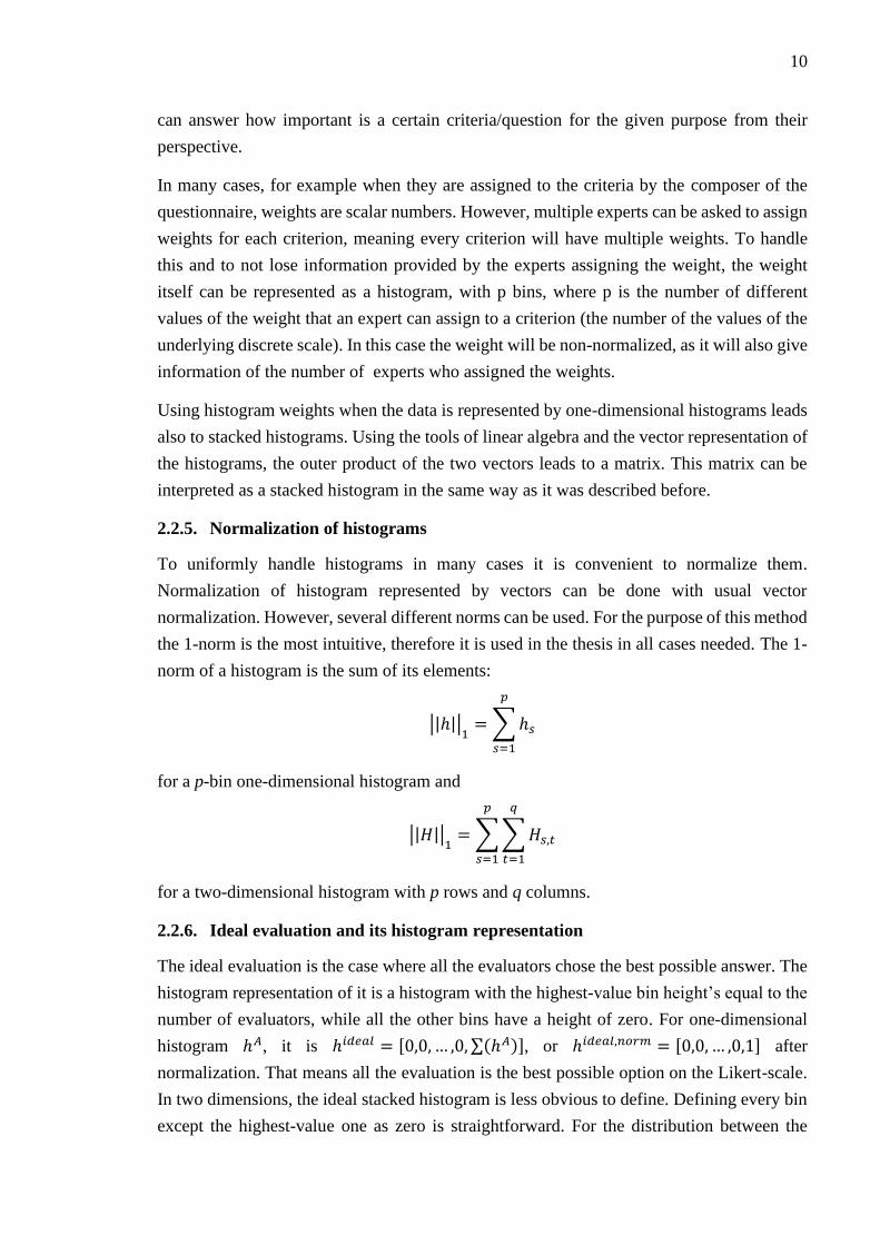
2.2.5. Normalization of histograms
To uniformly handle histograms in many cases it is convenient to normalize them.
Normalization of histogram represented by vectors can be done with usual vector
normalization. However, several different norms can be used. For the purpose of this method
the 1-norm is the most intuitive, therefore it is used in the thesis in all cases needed. The 1-
norm of a histogram is the sum of its elements:
||ℎ||1
= ∑ℎ𝑠
𝑝
𝑠=1
for a p-bin one-dimensional histogram and
||𝐻||1
= ∑∑𝐻𝑠,𝑡
𝑞
𝑡=1
𝑝
𝑠=1
for a two-dimensional histogram with p rows and q columns.
2.2.6. Ideal evaluation and its histogram representation
The ideal evaluation is the case where all the evaluators chose the best possible answer. The
histogram representation of it is a histogram with the highest-value bin height’s equal to the
number of evaluators, while all the other bins have a height of zero. For one-dimensional
histogram ℎ𝐴, it is ℎ𝑖𝑑𝑒𝑎𝑙 = [0,0, … ,0, ∑(ℎ𝐴)], or ℎ𝑖𝑑𝑒𝑎𝑙,𝑛𝑜𝑟𝑚 = [0,0, … ,0,1] after
normalization. That means all the evaluation is the best possible option on the Likert-scale.
In two dimensions, the ideal stacked histogram is less obvious to define. Defining every bin
except the highest-value one as zero is straightforward. For the distribution between the

11
importance levels, defining it as the same as the distribution of the evaluation histogram has,
i.e. using the same importance levels provided by the evaluators or experts for the criteria is
the most straightforward option. The reason for this is to allow the evaluations to be identical
to the ideal one. As all the evaluations have the same distribution between the importance
levels, if one evaluation’s histogram has only non-zero height in the last bin, it has to be the
histogram defined as the ideal. However, it is worth noting that the last bin (and only that
one) does not contribute to the Earthmover’s distance, as the distance-coefficient between
the bins (𝑝 − 𝑠) equals zero in the case of the highest-value bin.
Similarly, we can define the worst possible evaluation for both one- and two-dimensional
histograms. For one-dimensional histogram ℎ𝐴, it is ℎ𝑖𝑑𝑒𝑎𝑙 = [∑(ℎ𝐴) , 0, … ,0,0], or
ℎ𝑖𝑑𝑒𝑎𝑙,𝑛𝑜𝑟𝑚 = [1,0, … ,0,0] after normalization. That means all the evaluation is the best
possible option on the Likert-scale. For two-dimensional histograms, all rows except the first
(lowest-value bin) all of the elements are zeros. In the first rows the sum of the elements is
the same as the number of evaluators, and the distribution of them is same as the importance
levels. In that way, the first row of this stacked histogram will be the same as the last row of
the ideal evaluation histogram. The worst possible evaluation is really useful when the
distance from the ideal needed to be scaled between two numbers (0 and 1, in most cases, or
0 and 100 if one prefers using percentages), so it is easily understandable and comparable,
and independent of the number of evaluators or the weight histogram.
2.2.7. Distance between histograms
Measuring the distance between an arbitrary (ℎ𝐴) and the ideal (ℎ𝑖𝑑𝑒𝑎𝑙) histogram is very
important in the aggregation of the data, so the method of calculating it can make a big
difference. In this thesis we used the Earth-mover’s distance suggested in [5], introduced in
[14]. It is defined as the minimum number of steps to transform one histogram to the ideal
one, where one step means decreasing the height of a bin by one and increasing one of its
neighbor’s height by one.
For one-dimensional histograms:
𝑑(ℎ, ℎ𝑖𝑑𝑒𝑎𝑙) = ∑(𝑝 − 𝑠)(ℎ𝑠 − ℎ𝑠
𝑖𝑑𝑒𝑎𝑙)
𝑝
𝑠=1
(16)
For two-dimensional or stacked histograms:
𝑑(𝐻,𝐻𝑖𝑑𝑒𝑎𝑙) = ∑(𝑝 − 𝑠)[(𝐻𝑠,𝑖 − 𝐻𝑠,𝑖
𝑖𝑑𝑒𝑎𝑙) ∙ 𝑤]
𝑝
𝑠=1
(17)

12
with 𝑤 vector containing the importance levels or weights of the stacks and the ‘ ∙ ‘ operator
meaning the inner product of two vectors. The index 𝑖 is the running index, 𝐻𝑠,𝑖𝐴 meaning the
s-th bin of the histogram, that is in this case becomes a vector (i.e. the s-th row of 𝐻𝐴).
Using the above equations, it is possible to also define the distance between an arbitrary and
the worst possible histogram. The final evaluation value for a histogram is defined as its
distance from the ideal (calculated with the Earth-mover’s distance), divided by the
maximum possible distance, i.e. the Earth-mover’s distance between the ideal and the worst
possible evaluation, and the value subtracted from one. The last operation is for having
higher final evaluation score for better evaluations.
For one-dimensional case it is
𝑬 = 1 −
𝑑(ℎ, ℎ𝑖𝑑𝑒𝑎𝑙)
𝑑(ℎ𝑤𝑜𝑟𝑠𝑡, ℎ𝑖𝑑𝑒𝑎𝑙)
(18)
and for two-dimensional case
𝑬 = 1 −
𝑑(𝐻,𝐻𝑖𝑑𝑒𝑎𝑙)
𝑑(𝐻𝑤𝑜𝑟𝑠𝑡, 𝐻𝑖𝑑𝑒𝑎𝑙)
(19)
This provides final evaluation in the interval [0,1], with a higher value meaning a better
evaluation.
One might argue that the Earth-mover’s distance formula can be easily simplified for both
the one- and the two-dimensional cases. As the ideal histogram only has non-zero elements
in the last bin, but for that part of the summation (𝑝 − 𝑠) = 0, therefor it does not contribute
to the whole distance, we can simply leave the ideal histogram out from the formula. Also,
the last element in the summation can be (𝑝 − 1)th element for the same reason.
The simplified formulas for the Earth-mover’s distance for the one- and two-dimensional
cases, respectively:
𝑑(ℎ, ℎ𝑖𝑑𝑒𝑎𝑙) = ∑(𝑝 − 𝑠)
𝑝−1
𝑠=1
∗ ℎ𝑠
(20)
and

13
𝑑(𝐻,𝐻𝑖𝑑𝑒𝑎𝑙) = ∑(𝑝 − 𝑠)[𝐻𝑠,𝑖 ∙ 𝑤]
𝑝−1
𝑠=1
(21)
with 𝑤 vector containing the importance levels or weights of the stacks and the ‘ ∙ ‘ operator
meaning the inner product of two vectors. The index 𝑖 is the running index, 𝐻𝑠,𝑖 meaning the
s-th bin of the histogram, that is in this case becomes a vector.
Practically this means that we do not need to move any height from the last bin of the
evaluation histogram. However, it is better to define it the way as it was defined in (18) and
(19) for two reasons. One is that to emphasize that it is defined between an arbitrary and the
ideal histogram. The other is to keep it more general, in the case that another kind of ideal
need to be defined. In the scripts used for this thesis, the simplified versions of the formulas
were used, for computational efficiency purposes.
It is possible to define one-dimensional histograms as a special case of two-dimensional
ones, only having one importance value. This would mean that only the two-dimensional
case has to be defined and investigated for all formulas and methods. However, we think
that handling the one-dimensional case separately leads to easier understanding of the
methods and formulas used in the thesis.

14
3. Examples and visual description
3.1. Simple numerical examples
To provide numerical examples of the methods and formulas described, consider the
following problem.
𝑁 = 40 evaluators give answers to a question (e.g. in a questionnaire), with possible answers
being on a Likert-scale of (1, 2, 3, 4, 5). The histogram representing the Likert-type
evaluation data is ℎ = [16, 13, 8, 1, 2], meaning 16 evaluations of value 1, 13 of value 2, and
so on. The histogram is shown in Figure 1.
Now consider 15 experts providing importance levels for the question (criteria), with
possible values “not important”, “slightly important” or “important”. 4 experts said the
criterion is not important, 3 said it is slightly important, and 8 said it is important. This results
in a histogram weight 𝑤 = [4, 3, 8] for the question.
Now we can create a stacked histogram with 𝑤 and ℎ. It will result in a 2-dimensional
histogram, that we can represent with a matrix, calculating 𝐻 = ℎ𝑇 ∘ 𝑤𝑛𝑜𝑟𝑚, where
𝑤𝑛𝑜𝑟𝑚 =𝑤
||𝑤||1
= [4
15,
3
15,
8
15] is the normalized form of 𝑤, so it shows the ratio between the
number of evaluations in different categories. This way, we get
𝐻 = ℎ𝑇 ∘ 𝑤𝑛𝑜𝑟𝑚 = [16, 13, 8, 1, 2]𝑇 ∘ [4
15,
3
15,
8
15] =
[ 4.27 3.20 8.533.47 2.60 6.932.13 1.60 4.270.27 0.20 0.530.53 0.40 1.07]
.
Visualizing the one-dimensional evaluation histogram:

15
Figure 1 Example 1 dimensional histogram ℎ = [16, 13, 8, 1, 2]
For the purpose of visualization, the stacked histogram is rotated, so the bin values will be
on the 𝑥-axis, and the bin heights on the 𝑦-axis.

16
Figure 2 Example stacked histogram 𝐻 =
[ 4.27 3.20 8.533.47 2.60 6.932.13 1.60 4.270.27 0.20 0.530.53 0.40 1.07]
𝑇
Now we will show that destacking the histogram works in a way that it gives back the two
original histograms that were used to create it. First, let us consider the row-wise sum of 𝐻.
Σ(𝐻, 1) = [𝐻1,1 + 𝐻1,2 + 𝐻1,3, … , 𝐻5,1 + 𝐻5,2 + 𝐻5,3]𝑇
= [16, 13, 8, 1, 2]𝑇 = ℎ𝑇, so we
successfully recreated the original one-dimensional evaluation histogram. Now with the
column-wise sum Σ(𝐻, 2) = [𝐻1,1 + 𝐻2,1 + ⋯+ 𝐻5,1, … , 𝐻1,3 + 𝐻2,3 + ⋯+ 𝐻5,3] =
[32
3,24
3,64
3] = 𝑤2. This is not the original weight histogram, however after normalizing it,
we get 𝑤2,𝑛𝑜𝑟𝑚 = [32
120,
24
120,
64
120] = [
4
15,
3
15,
8
15] = 𝑤𝑛𝑜𝑟𝑚, so the ratios between the weight
bins (or importance levels) are the same as in the original weight histogram. If the number
of experts, i.e. the sum of the original weight histogram is known, then the non-normalized
original weight histogram can be calculated.
For a more compound example, first consider another criterion, and then a second alternative
that has the same two criteria evaluated by the same group of people.
Suppose that we have two travel agencies A and B, that are evaluated by the same 40 people,
by the same two criteria. Let the first criterion be “Customer service availability” and the
second is “Simplicity of booking”, both evaluated on Likert-scale with values of 1,2,3,4 and

17
5, 1 being the worst and 5 being the best. The evaluation given by the 40 people are below,
𝑒𝐴𝑖 meaning the evaluation of travel agencies A w.r.t. to the i-th criterion and 𝑒𝐵𝑖 meaning
the evaluation of travel agencies B w.r.t. to the i-th criterion.
𝑒𝐴1 = [16, 13, 8, 1, 2]𝑇
𝑒𝐴2 = [2, 1, 8, 15, 14]𝑇
𝑒𝐵1 = [3, 4, 7, 12, 14]𝑇
𝑒𝐵2 = [4, 5, 10, 9, 12]𝑇.
The evaluation histograms are visualized in Figure 3.
The importance levels (on the scale of (1,2,3)) provided by 15 experts for the two criteria
are
𝑤1 = [4, 3, 8]
𝑤2 = [6, 6, 3].
The weight histograms are visualized in Figure 4. The y-axis, “Number of experts”, shows
how many experts gave a certain weight value for the specific criterion.
Figure 3 Evaluation histograms of both travel agencies w.r.t. both criteria

18
Figure 4 Weight histograms for both criteria
First, we need to have evaluation for both alternatives. That is achieved by the weighted
average of the two evaluations for the different criteria. This results in two 2-dimensional
histograms, one for each alternative:
𝑒𝐴 =(𝑒𝐴1 ∘ w1, 𝑛𝑜𝑟𝑚 + 𝑒𝐴2 ∘ w2, 𝑛𝑜𝑟𝑚)
2
=[16, 13, 8, 1, 2]𝑇 ∘ [
415
, 315
, 815
] + [2, 1, 8, 15, 14]𝑇 ∘ [615
, 615
, 315
]
2
=
[ 2.53 2.00 4.471.93 1.50 3.572.67 2.40 2.933.13 3.10 1.773.07 3.00 1.93]

19
𝑒𝐵 =(𝑒B1 ∘ w1,𝑛𝑜𝑟𝑚 + 𝑒B2 ∘ w2,𝑛𝑜𝑟𝑚)
2
=[3, 4, 7, 12, 14]𝑇 ∘ [
415
, 315
, 815
] + [4, 5, 10, 9, 12]𝑇 ∘ [615
, 615
, 315
]
2
==
[ 1.20 1.10 1.201.53 1.40 1.572.93 2.70 2.873.40 3.00 4.104.27 3.80 4.93]
The stacked histograms representing 𝑒𝐴 and 𝑒𝐵 are shown in Figure 5.
Figure 5 Stacked histograms of the two alternatives in the example
The heights of the bins are not necessarily integers, because of the averaging. However, since
we have normalized the weight histograms before calculating the weighted average, the sum
of the height of the bins gives the total number of evaluators (40) for both stacked
histograms.
We define the ideal and the worst histogram according to section 2.1. With this, the ideal
becomes:
𝐻𝑖𝑑𝑒𝑎𝑙 =
[
0 0 00 0 00 0 00 0 0
15.35 15.0 9.65]

20
and the worst histogram:
𝐻𝑤𝑜𝑟𝑠𝑡 =
[ 15.35 15.0 9.65
0 0 00 0 00 0 00 0 0 ]
Now, with the ideal and the worst stacked histogram being defined, we can continue the
example with calculating the distances from the ideal histogram for the two alternatives with
equation (16). For alternative A, the distance from the ideal is
𝑑𝐴 = 1101.1
while for alternative B,
𝑑𝐵 = 736.4
That means, as alternative B is closer to the ideal alternative, it is better than alternative A,
considering these criteria and weight set. However, these numbers are not really intuitive,
and do not give any idea of the differences and magnitude of the distances. Dividing the
calculated distances by the maximum possible distance
𝑑𝑚ax = d(𝐻𝑖𝑑𝑒𝑎𝑙 , 𝐻𝑤𝑜𝑟𝑠𝑡) = 2147.6
we get the final evaluations with equation (18) for both alternatives (rounded to two
decimals):
𝑬𝑨 = 1 −𝑑𝐵
𝑑𝑚𝑎𝑥= 0.49
𝑬𝑩 = 1 −𝑑𝐵
𝑑𝑚𝑎𝑥= 0.68
Comparing these values to the histograms in Figure 5, alternative A being middle evaluated
(final evaluation score close to 0.5) seems fitting for the distribution of the values between
the bins. For alternative B it is clear that is better than A, and their final evaluation scores
shows the difference between them.
Thinking about the acquisition of the weight histograms, two possible ways were mentioned
in 2.1, Weights. However, one seemingly more complex case can be when weight (or in this
case, more intuitively, importance) histograms come from both experts and evaluators.
Applying the method for stacking shown in section 2.1, one could create a three-dimensional
matrix, similarly for the two-dimensional case. The proportion of the values in the three
dimensions would represent the distribution of the total evaluation, the importances from the
first source, and the importances from the second source. The size of this matrix would be
21
𝑝 × 𝑞 × 𝑟, where p, q, r are the sizes of the Liker-scales for the evaluation, the first, and the
second source of importance histograms, respectively.
However, the handling of these matrices would be more complex than of the two-
dimensional ones. Without any constraint for generality, we can assume that the two sources
of importances are using the same Likert-scales, i.e. 𝑞 = 𝑟. From these two histograms we
can create an overall weight histogram by averaging those two histograms. With the overall
weight histogram, now we can create the two-dimensional histograms the same way as
before. It is easy to see that this aggregation of weight histograms can be generalized to an
arbitrary number of weight histograms, keeping the same assumption of their Likert-scales.
However, the drawback of this method is the loss off information when averaging the weight
histograms. To keep the algorithm lossless, we need to keep one of the original histograms,
so we can restore the other one with the average weight. In the general case of multiple
weight histograms, we need to keep all except one to be able to restore all the original
histogram.
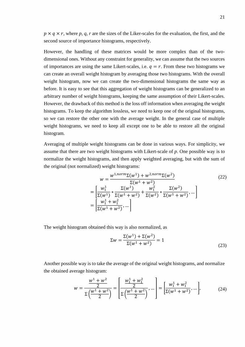
Averaging of multiple weight histograms can be done in various ways. For simplicity, we
assume that there are two weight histograms with Likert-scale of p. One possible way is to
normalize the weight histograms, and then apply weighted averaging, but with the sum of
the original (not normalized) weight histograms:
𝑤 =𝑤1,𝑛𝑜𝑟𝑚Σ(𝑤1) + 𝑤2,𝑛𝑜𝑟𝑚Σ(𝑤2)
Σ(𝑤1 + 𝑤2)
= [𝑤1
1
Σ(𝑤1)∗
Σ(𝑤1)
Σ(𝑤1 + 𝑤2)+
𝑤12
Σ(𝑤2)∗
Σ(𝑤2)
Σ(𝑤1 + 𝑤2), … ]
= [𝑤1
1 + 𝑤12
Σ(𝑤1 + 𝑤2), … ]
(22)
The weight histogram obtained this way is also normalized, as
Σ𝑤 =Σ(𝑤1) + Σ(𝑤2)
Σ(𝑤1 + 𝑤2)= 1
(23)
Another possible way is to take the average of the original weight histograms, and normalize
the obtained average histogram:
𝑤 =
𝑤1 + 𝑤2
2
Σ (𝑤1 + 𝑤2
2)
= [
𝑤11 + 𝑤1
2
2
Σ (𝑤1 + 𝑤2
2)
, … ] = [𝑤1
1 + 𝑤12
Σ(𝑤1 + 𝑤2), … ],
(24)

22
using that the division by 2 can be applied outside of the summation. It is clear that these
two methods provide the same, normalized result. It is easy to see that also adding the two
histograms and normalizing it will lead to the same formula.
For an example of weight aggregation, let us start from two 3-bin weight histograms, 𝑤1 =
[4, 3, 8] and 𝑤2 = [4, 6, 5], with possible weight values (1,2,3). They are plotted in Figure
6. Then, calculating the aggregated weight with the previous equation (since the two methods
lead to the same result, it doesn’t matter which one we are using) the overall weight
histogram is 𝑤𝑜𝑣𝑒𝑟𝑎𝑙𝑙 = [8
30,
9
30,13
30] ≅ [0.267, 0.3, 0.433] (see on Figure 7).
Figure 6 Example weight histograms

23
Figure 7 Example overall weight histogram
Comparing the original and the aggregated histograms, it is easy to see that both of the
originals represent higher weighted criteria than average, and it also shows in the aggregated
weight. The result might be easier to interpret if we do not normalize, but just calculate the
average of the two not normalized original histogram (or rescale the result to the same
summed height of the bins). That way we get 𝑤𝑎𝑣𝑒𝑟𝑎𝑔𝑒 = [4, 4.5, 7.5]. This might be easier
to compare to the original weights, and useful if one needs not-normalized weight
histograms.
It is also possible to come up with the case where we have a stacked evaluation histogram,
and we have weight histogram for that criterion. This can happen in the case when all the
evaluators also rated the importance of the criterion, while experts gave importance levels,
too. Simply applying the weight is not straightforward (if we do not want to use three-
dimensional histograms) but creating weight histogram (or histograms) from the stacked one
is a way to have multiple histogram weights and aggregate them just as before. The problem
in this case is that the stacked histogram was not created from separate weight and
evaluation, therefore the destacking method described above does not work. That means that
the bins of the histogram have different distribution on the Likert-scale of the weights, or
different ratio between the important values).
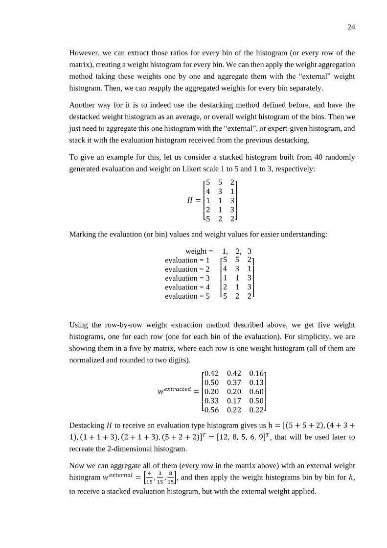
24
However, we can extract those ratios for every bin of the histogram (or every row of the
matrix), creating a weight histogram for every bin. We can then apply the weight aggregation
method taking these weights one by one and aggregate them with the “external” weight
histogram. Then, we can reapply the aggregated weights for every bin separately.
Another way for it is to indeed use the destacking method defined before, and have the
destacked weight histogram as an average, or overall weight histogram of the bins. Then we
just need to aggregate this one histogram with the “external”, or expert-given histogram, and
stack it with the evaluation histogram received from the previous destacking.
To give an example for this, let us consider a stacked histogram built from 40 randomly
generated evaluation and weight on Likert scale 1 to 5 and 1 to 3, respectively:
𝐻 =
[ 5 5 24 3 11 1 32 1 35 2 2]
Marking the evaluation (or bin) values and weight values for easier understanding:
weight = 1, 2, 3
evaluation = 1
evaluation = 2
evaluation = 3
evaluation = 4
evaluation = 5 [ 5 5 24 3 11 1 32 1 35 2 2]
Using the row-by-row weight extraction method described above, we get five weight
histograms, one for each row (one for each bin of the evaluation). For simplicity, we are
showing them in a five by matrix, where each row is one weight histogram (all of them are
normalized and rounded to two digits).
𝑤𝑒𝑥𝑡𝑟𝑎𝑐𝑡𝑒𝑑 =
[ 0.42 0.42 0.160.50 0.37 0.130.20 0.20 0.600.33 0.17 0.500.56 0.22 0.22]
Destacking 𝐻 to receive an evaluation type histogram gives us h = [(5 + 5 + 2), (4 + 3 +
1), (1 + 1 + 3), (2 + 1 + 3), (5 + 2 + 2)]𝑇 = [12, 8, 5, 6, 9]𝑇, that will be used later to
recreate the 2-dimensional histogram.
Now we can aggregate all of them (every row in the matrix above) with an external weight
histogram 𝑤𝑒𝑥𝑡𝑒𝑟𝑛𝑎𝑙 = [4
15,
3
15,
8
15], and then apply the weight histograms bin by bin for ℎ,
to receive a stacked evaluation histogram, but with the external weight applied.

25
Destacking 𝐻 according to (15) provides and average weight histogram 𝑤𝑎𝑣𝑔 =
[0.43, 0.3, 0.27]. We can aggregate it with the external weight used above, and then restack
it with ℎ as evaluation. The two restacked histograms are shown below in Figure 8.
Figure 8 Restacked histograms using the average and row-by-row weighting method (left) and external
weight histogram (right)
Though they are clearly different, it is probably easier to see the difference between the two
methods, if we just restack the extracted weights with ℎ, without applying an external weight
histogram. The result from both methods, along with the original 𝐻 stacked histogram is
shown below.
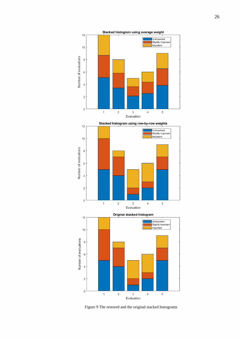
26
Figure 9 The restored and the original stacked histograms

27
The row-by-row weighting method gives back the original 2-dimensional histogram, while
using the average weight of the bins distorts it. Thus, we can claim the row-by-row
destacking method is lossless (as long as we do not apply aggregation with an external
weight).
3.2. Description
The dataset from [15] that is used to demonstrate the method is from Palacký University
Olomouc in Czech Republic and contains anonymous information from tests and a survey
among students. The table consist of the following fields:
• ID of the student (integers between 1 and 140)
• Form of study (standard or combined/remote)
• University entrance exam score (maximum score is 100)
• High school graduation exam grade average (1 is best, 5 is worst)
• Age
• Sex
• Survey of 30 self-assessment scores (described below)
Both the University entrance exam score and the High school graduation grade average are
missing for some students. The survey consisted of 30 questions, that were grouped into 5
different groups:
• Reading and writing (denoted by “A”, 5 questions)
• Research and structure (denoted by “B”, 5 questions)
• Future practice (denoted by “C”, 5 questions)
• Theory (denoted by “D”, 9 questions)
• Critical thinking and curiosity (denoted by “E”, 6 questions)
We refer to these groups of questions (from A to E) as ‘criteria’, while to the questions as
‘subcriteria’. Each student answered each question, on a 4-point Likert-scale coded wit
0=”completely not fitting”, 1=”somehow not fitting”, 2=”somehow fitting” and
3=”completely fitting”.
The work of Stoklasa et al. [15] uses fuzzy methods and coverage measures in the processing
of the same dataset. In this conference paper the authors are aiming for success and failure
prediction in academic fields and optimizing university assessment methods and exams.

28
After converting the dataset so it is easy to read with MATLAB®, we have analyzed it with
the methods described before. Our goal was to rank the students, and compare the results to
other ranking methods, then conclude differences and similarities of the rankings.
3.3. Results
3.4. Analysis using one-dimensional weights
First, we created the histograms for every student, with respect to all criteria. These
histograms have a total bin height of the number of subcriteria in the corresponding criteria.
For the first analysis we were using scalar weights, each criterion having the weight equal
to the number of subcriteria it contains. Then we calculated the average histogram for every
student. Since we have not yet normalized the histograms, we could just simply add them
and divide by 5 (the number of criteria). This way every student has one histogram assigned,
that has a total bin height of 6, since this is the average number of subcriteria in one criterion.
An example is shown on Figure 10.
Figure 10 Example evaluation histogram for a student

29
For evaluating the students, we needed the distance from the ideal histogram for all of them.
This is defined as
ℎ𝑖𝑑𝑒𝑎𝑙 = [0,0,0,0,6]
and we also defined the worst possible evaluation, that was needed to scale the distances as
ℎ𝑤𝑜𝑟𝑠𝑡 = [6,0,0,0,0]
according to 2.1. Then we could calculate the distance from the ideal for every student using
the Earth-mover’s distance (16). Using the formula (18), we calculated the final evaluation
score for all students. The final evaluation scores are visualized (in ascending order) on
Figure 11.
Figure 11 Scaled distances for all students (in ascending order)
We compared the final evaluation scores to the entrance exam scores, with transforming the
entrance exam scores to the same scale. For that we divided the entrance exam scores with
100 (the maximum possible score). The comparison is show in Figure 12. The students are
ordered by their scores of evaluation/entrance exam as in the previous figure, so the value
on x-axis does not identify one certain student.
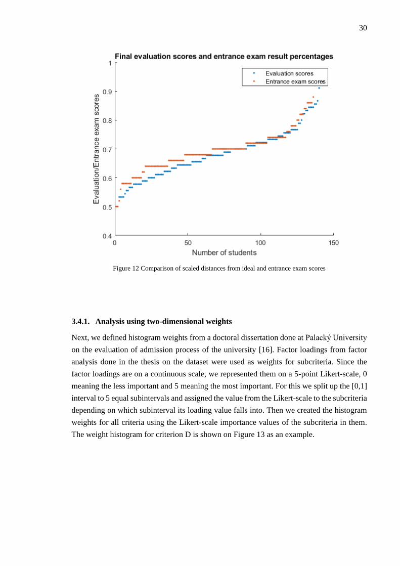
30
Figure 12 Comparison of scaled distances from ideal and entrance exam scores
3.4.1. Analysis using two-dimensional weights
Next, we defined histogram weights from a doctoral dissertation done at Palacký University
on the evaluation of admission process of the university [16]. Factor loadings from factor
analysis done in the thesis on the dataset were used as weights for subcriteria. Since the
factor loadings are on a continuous scale, we represented them on a 5-point Likert-scale, 0
meaning the less important and 5 meaning the most important. For this we split up the [0,1]
interval to 5 equal subintervals and assigned the value from the Likert-scale to the subcriteria
depending on which subinterval its loading value falls into. Then we created the histogram
weights for all criteria using the Likert-scale importance values of the subcriteria in them.
The weight histogram for criterion D is shown on Figure 13 as an example.

31
Figure 13 Weight histogram for criterion D
Stacked histograms were created for every student, stacking the evaluation histogram
obtained from the self-evaluation scores and the weight histogram. This resulted in 5
histograms for every student, one for each criterion. Therefore, we averaged the histograms
student-by-student, to have one evaluation for every one of them. For that we simply added
the histograms and divided by five, since the histograms were not yet normalized. An
example is visualized in Figure 14.

32
Figure 14 Stacked histogram for student with ID of 69, w.r.t criterion E
Then we created the ideal and worst histograms:
ℎ𝑖𝑑𝑒𝑎𝑙 =
[ 0 0 0 0 00 0 0 0 00 0 0 0 00 0 0 0 00 4.8 17.8 13.8 2.0]
ℎ𝑤𝑜𝑟𝑠𝑡 =
[ 0 4.8 17.8 13.8 2.00 0 0 0 00 0 0 0 00 0 0 0 00 0 0 0 0 ]
Then similarly as before, we calculated the distance from the ideal for all student’s
evaluation histogram, as well as for the worst possible evaluation, this time using the two-
dimensional Earth-mover’s distance (17), and from that the final evaluations using (19). A
comparison to the evaluation scores calculated in the previous section is shown in Figure 15.
The students are ordered by their scores of evaluation/entrance exam, so the value on x-axis
does not identify one certain student.

33
Figure 15 Final evaluation scores using the two proposed methods (in ascending order)
3.4.2. Correlation of the exam results and the evaluations
We can define the ranking of the students based on four grading, or evaluation: the university
entrance exam score, the high school graduation exam average grade and the final evaluation
score of the two methods used in the thesis. We could calculate the rank correlation between
rankings based on different measures, however this does not lead to useful results because
of the high number of repeating values in each column. The students only have 18 different
graduation exam average scores and 20 different entrance exam scores. Students with the
same score can be ranked arbitrarily, which makes the ranking useless. (Not counting
missing data.)
However, examining the values of final evaluations provided by the method proposed in this
thesis, the method using scalar weights gives 40 different values, while the evaluation using
histogram weights gives 19 different final evaluation values. This shows the differentiating
feature of the methods: the more different the values assigned to the students, the easier to
rank them.
For the abovementioned reason, we divided the students into groups based on their rankings
in the following way: students who had the highest score with respect to a certain criterion
(all ranked as first) were assigned to group one, those who had the second highest score were

34
assigned to group and so on. Then we calculated how many students fall into the first n group
(groups from 1 to n), i.e. into the first group alone, then into the first and second group and
so on, until all 140 of the student were covered (excluding students with missing scores).
We did this grouping with respect to the graduation exam average grade and the entrance
exam scores. The number of students falling into the first n group are shown in Figure 16.
he maximum of the number of students are different due to the different number of missing
scores on the two rankings.
Figure 16 Cumulative number of students in the groups
In the next step we calculated overlapping of the rankings with the help of these groups.
First, we calculated the overlapping between the students in the first group with respect to
the graduation exam and the same number of students who were ranked highest with respect
to our methods (one by one). Then we did the same with the first two groups, and so on. We
excluded students with missing scores in the graduation exams from the evaluation ranking,
too. We calculated the overlapping percentage between the graduation exam rankings and
both evaluation methods, one by one. The percentage of the overlapping students are show
in Figure 17.
35
Figure 17 Overlap percentage between graduation exam ranking and the evaluation methods
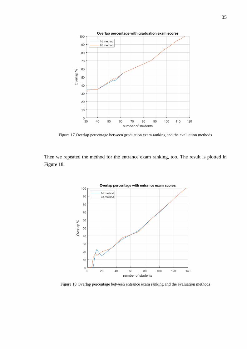
Then we repeated the method for the entrance exam ranking, too. The result is plotted in
Figure 18.
Figure 18 Overlap percentage between entrance exam ranking and the evaluation methods

36
The overlap percentage for the entrance exam ranking starts at a very low value, because the
first few groups contain very low number of students (few students getting high scores),
while in the graduation a much larger number of students had high average grade.
In these examinations an important point is the overlap percentage at 60 students, because
the university accepts the top 60 students based on the entrance exam. Overlap percentage
of slightly above forty (about 25 students) is lower that one could expect. This means that
based on the evaluation methods, it can be estimated that only 25 of the accepted 60 students
are actually among the best 60. The interpolation between the exact number of students in
the groups (there is no overlap percentage calculation exactly at 60 students) leads to a little
inaccuracy.
We also calculated the overlap percentage of students between the two analysis, using 1-
dimensional and 2-dimensional weights. The result is plotted in Figure 19.
Figure 19 Overlap percentage between the evaluation methods
The overlap percentage between the two methods (using one-dimensional and two-
dimensional) weights are close to 100%, regardless of how many groups we are considering.
The higher values than the previous comparisons are somewhat expected, as the two analysis
were based on the same dataset. The small differences in the ranking shows that the assigned
weights play an important role in the analysis methods, and can have a some effects in the
final ranking.

37
An important note is that the final evaluation ranking also has some inaccuracy due to
students scoring the same scores and therefore ranked same. This leads to occasionally
“cutting” groups when taking a certain number of students from the beginning of the ranking.
However, the groups containing much less students in these rankings than the ordering based
on the exams (due to a higher number of different scores), therefore it is not causing a
noticeable flaw in the results. Given that the 1d method has 38 different scores, it has average
3.7 students in a group, which leads to an average of less than 2 students, when randomly
cutting it, producing about 3% error in the case of 60 students. In the case of the 2d method,
the 138 different final evaluation score can be approximated that all the students have
different scores, causing an error of close to 0 in the overlap analysis.
Other possible inaccuracies of the analysis are discussed in more detail in chapter 4.1.
The score correlations between the different rankings are shown in Table 1. We used
Spearman’s correlation method, due to the self-assessment scores being on ordinal scale.
Evaluation
method
Scalar weight Histogram
weight
Graduation
exam
Entrance exam
Scalar weight 1 0.998 0.060 0.147
Histogram
weight
0.998 1 0.041 0.141
Graduation exam 0.060 0.041 1 0.152
Entrance exam 0.145 0.141 0.152 1 Table 1 Correlation between the evaluation methods
The table is trivially symmetric to its diagonal, since the correlation does not depend on the
order of the two inputs that it calculates the correlation for.
The diagonal elements are trivially one, but the correlation between the two variant of the
method we introduced and used in the thesis being close to one means that the final
evaluation of the two methods produce similar ranking for the students.
The correlation between the proposed methods and the two exams the students took, are the
most interesting and important ones. The proposed methods’ correlation with the university
entrance exam scores is almost twice as high as the correlation with the high school
graduation exam averages. There is also a slight difference between using histogram weights
and scalar weights, the method with histogram weights producing higher correlation to both
exams’ results.

38
The final value not yet examined, the correlation between the scores between the high school
graduation and the university entrance exams is in the same range as the self-assessment
evaluation’s correlation to the university entrance exam.

39
4. Discussion
4.1. Current Study
The outcomes show that the methods provide meaningful results when analyzing Likert-
scale data. It was also shown that the methods provide a reduce in information loss, as until
the final aggregation the original dataset was reproducible given the number of evaluators
and experts (i.e. the total bin heights of the original histograms).
Comparison between the methods using one- and two-dimensional weights showed the
effect of choosing weights for the analysis, as it can alter the final results. However, the two
methods were still consequent to each other, but comparing them to the exam results showed
low correlation.
4.1.1. Limitations of the study
It is important to discuss the limitations of the work to see why the results are needed to be
interpreted with caution.
The data used in the analysis comes from a self-evaluation questionnaire, and as such the
given answers can easily be biased. However, the direction of the bias cannot be determined,
as every student are evaluating themselves differently, either in a more strict or lenient way
compared to others. On the other hand, for the purpose of the thesis it was sufficient, as one
of the intended results of the analysis was to examine the effectiveness of the earlier rankings
based on exams. Using another exam to compare might have been less sensible in this case.
Another source of error comes from the construction of the original data. Why one should
handle the original data thoughtfully has several reasons:
• the filling of the questionnaire was voluntary,
• only students that were accepted by the entrance exams (and studied at the university
for some time) were asked,
• not all of the students are from the same grade, so they have written different
graduation and entrance exams.
What bias can these reasons cause exactly are out of the scope of this thesis, but we thought
it is beneficial to mention of some possibilities. The voluntariness of the returning of the
questionnaire might cause that only the better performing students are in the study, as one
with lower performance might not willingly discuss their performance (even anonymously).
Asking only the accepted students obviously excludes the students with low score on the
entrance exam, distorting the result of the analysis of how predictive the entrance exam score
on the future success of a student is. Finally, having students with different graduation year

40
means that one who finished highly ranked in their year can ranked lower overall, if they
had to do a harder than average exam, leading to lower scores than students doing the exams
in a different year.
4.2. Future Work
4.2.1. Generalization of the proposed methods
If we do not assume that the Likert-scale used to acquire the histograms are equidistant, the
Earth-mover’s distance (formulas (16) and (17)) defined in section 2.1 cannot give any
sensible results. However, if we assume that we know exactly the distance between the bins,
we can modify it by including them in the formula:
𝑑(ℎ, ℎ𝑖𝑑𝑒𝑎𝑙) = ∑ 𝑑𝑠 ∗ (ℎ𝑠 − ℎ𝑠
𝑖𝑑𝑒𝑎𝑙)
𝑝
𝑠=1
(25)
for one-dimensional and
𝑑(𝐻,𝐻𝑖𝑑𝑒𝑎𝑙) = ∑𝑑𝑠 ∗ [(𝐻𝑠,𝑖 − 𝐻𝑠,𝑖
𝑖𝑑𝑒𝑎𝑙) ∙ 𝑤]
𝑝
𝑠=1
(26)
for two-dimensional histograms.
where 𝑑𝑠 is the distance of the s-th bin from the highest-value bin. This simply means we
need to move this bin’s value not with (𝑝 − 𝑠) steps to reach the highest-value bin, but with
the distance between them. In other words, instead of weighting the values of the bins (or
more exactly, the differences between the values of the bins) with 1, we weight it with some
predefined distance between them.
On the other hand, in many cases it cannot be assumed that we know the exact distances
between the bins. For example, with using linguistic labels for the Likert-scale, we cannot
be sure the labels mean the same for different evaluators. However, the assumption that the
scale is symmetrical, i.e. the distance between the first and second, and the distance between
the last and second to last bins are equal, we can simplify the histogram. The method for it
is to create a 3-bin histogram, where the height of the first bin is the sum of the heights of
all bins below the middle one, and the height of the last (third) bin is the sum of the heights
of all the bins above the middle one. (For histograms with even number bins on can create a
two-bin histogram with the similar method.) This can be assumed as equidistance because
of the symmetry of the original histogram.
The 3-bin equidistant histogram can be handled by the method introduced in the thesis;
however, the question of information loss arises. As some bins were aggregated, and just
from the summed value of them they cannot be restored, we lost some information during

41
this method, namely the distribution of the evaluations below and above average. However,
if we know nothing about the distances between those bins, we actually do not know the
distribution of their values originally, so it is more sensible to talk about data loss, rather
than information loss in this case.

42
5. Conclusion
We have shown that the proposed method is a practical way for representing data on Likert-
scale. The method can be used to handle various type of data, including scalar and histogram
weights, and one- and two-dimensional histograms, making it a widely usable tool for data
representation and evaluation. We proposed further possible way of generalization, that can
make the method even more flexible to varying datasets.
Though the method does not provide a fully lossless representation as the final aggregation
of the data needs to lead to a simple and easily interpretable result, in major part of the
method we were able to keep the amount of lost information at a very low level.
The demonstration using the dataset provided by Palacký University showed the method is
worth using on real datasets in the future.

43
References
[1] P. A. Bishop és R. L. Herron, „Use and Misuse of the Likert Item Responses and Other
Ordinal Measures,” International Journal of Exercise Science, p. 297–302., 2015.
[2] R. Likert, „A technique for the measurement of attitudes,” Archives of Psychology,
1932.
[3] J. Stoklasa, T. Talášek, J. Kubátová and K. Seitlová, "Likert Scales in Group Multiple-
criteria Evaluation," Journal of Mult.-Valued Logic & Soft Computing, p. 425, 2017.
[4] T. D. e. a. Shanafelt, „Impact of Organizational Leadership on Physician,” Journal of
Services Marketing, 2009.
[5] G. Hoang, J. Stoklasa and T. Talášek, "First steps towards lossless representation of
questionnaire data and its aggregation in social science and marketing research," p.
112, 2018.
[6] J. Stoklasa, T. Talášek and P. Luukka, "Fuzzified Likert Scales in Group Multiple-
Criteria Evaluation," p. 165, 2018.
[7] J. T. Croasmun és L. Ostrom, „Using Likert-Type Scales in the Social Sciences,”
Journal of Adult Education, 2011.
[8] L. Hall, C. Hume és S. Tazziman, „Five Degrees of Happiness: Effective Smiley Face
Likert,” 2016.
[9] K. Kurtulus, S. Kurtulus és Z. Bozbay, „Research Methodology in Marketing
Publications: Review and Evaluation,” in 6th International Multi-Conference on
Society, Cybernetics and Informatics, Orlando, Florida USA, 2012.
[10] A. K. M. K. e. a. Pervez, „Fuzzy-Likert scale based assessment of marketing risk faced
by the hybrid rice growers of Bangladesh,” Economics of Agriculture, 2019.
[11] T. e. a. Harada, „Five-point Likert scaling on MRI predicts clinically significant
prostate carcinoma,” BioMed Central, 2015.
[12] C. K. e. a. Weber, „The five-point Likert scale for dyspnea can properly assess the
degree of pulmonary congestion and predict adverse events in heart failure
outpatients,” Clinics, 2014.

44
[13] Q. Li, "A novel Likert scale based on fuzzy sets theory," Expert Systems with
Applications, p. 1609, 2013.
[14] Y. Rubner, C. Tomasi and L. J. Guibas, "A Metric for Distributions with Applications
to Image Databases," 1998.
[15] J. Stoklasa, T. Talášek and L. Viktorová, "Do we have crystal balls? A case study of
the possibility of predicting academic," Palacký University Olomouc, 2020.
[16] L. Viktorová, Evaluation of the admission process for Psychology at the Faculty of
Arts, Palacký University, from the perspective of academic success, 2018.