bending vibrational data accuracy … computation speed of the program is less than that required...

b J

BENDING VIBRATIONAL DATA ACCURACY STUDY

TECHNICAL REPORT NO. 70-1066

SEPTEMBER 1970

BY

J. H. WIGGINS COMPANY

Palos Verdes Estates,

California 90274

Prepared For

GEORGE C. MARSHALL SPACE FLIGHT CENTER

NATIONAL AERONAUTICS AND SPACE ADM l N ISTRATION MARSHALL SPACE FLIGHT CENTER

Alabama 3581 2

Under Contract NAS8-25458

* h

https://ntrs.nasa.gov/search.jsp?R=19710005720 2018-08-31T02:13:35+00:00Z

BEND I NG V I B R A T I O N A L

DATA ACCURACY STUDY

Jon D . C o l l i n s Bruce Kennedy Gary C . Har t

prepared by

J . H. Wiggins Co. Palos Verdes E s t a t e s

C a l i f o r n i a

f o r

George C . Marshal l Space F l i g h t Center

September 9970

FOREWORD

This project was sponsored by the George C. Marshall Space Flight Center under NASA Contract NAS8-25458. The work was performed under the technical direction of Larry A. Kiefling, MSFC Code S & E-Aero-DDS.

We wish to express our appreciation to Mr. Kiefling for his thoughtful contributions to the partial derivative development.

TABLE OF CONTENTS

1.0 INTRODUCTION AND SUMMARY 1-1

2.0 PROCEDURE 2-1

2.1 Statistical Background 2-1 2.2 Considerations in the Dynamic

Model 2-2 2.3 Statistical Development 2-4 2.4 Implementation of the Statistical

Model 2-9

3.0 EIGENVALUE AND EIGENVECTOR PARTIAL DERIVATIVES 3-1

3.1 Eigenvalue Partial Derivatives 3-1 3.2 Eigenvector Partial Derivatives 3-3

4.0 ELEMENT PROPERTY SENSITIVITY MATRICES 4-1

4.1 Beam Element 4.2 Plate Element 4.3 General Stiffness Matrix

5.0 PROPERTY COVARIANCE MATRICES 5-1

5.1 Introduction 5-1 5.2 Development of a Property Covariance

Matrix for a Tubular Beam Element 5-2 5.3 Development of a Property Covariance

Matrix for a Sandwich Plate Element 5-5

6.0 SYNTHESIS 6-1

6.1 Construction of the Mass and Stiffness Matrices 6-1

6.2 Compatibility 6-3 6.3 The Solution of Eigenvector

Partial Derivatives 6-14 6.4 Program Operation 6-17

7.0 EXAMPLES AND VERIFICATION 7-1

7.1 Methodology 7-1 7-2 Four Degree-of-Freedom Longitudinal

Vibrations 7-1 7 - 3 S I1 Longitudinal Vibration 7-11

8.0 CONCLUSIONS AND RECOWENDATTONS 8 - 1

REFERENCES

APPENDIX A - Nomenclature APPENDIX B - User's Manual

1.0 I NTRODUCT I ON AND SUMMARY

This report presents the theory and describes the operation of a computer program designed to predict uncertainty in structural modal characteristics based on uncertainty in structural physical properties. The program, entitled VIDAP (Vibrational Data Accuracy Program), can handle both stiffness and mass uncertainty and can work with an arbitrary stiffness matrix or one which involves beam or plate elements. The program and the supporting theory have the following features:

a linear statistical model which can accurately predict uncertainties of selected frequencies and modes based on the uncertainty in properties of individual elements.

the program never handles matrices of dimension larger than the total degrees of freedom of the system. The program can handle problems of up to 300 degrees of freedom.

the computation speed of the program is less than that required for computation of eigenvectors and eigenvalues.

tl:e program stands alone from any structural dynamics program, requiring only the eigenvalues and eigenvectors, the mass and stiffness matrices, and certain element properties as input.

the input procedure is cP such a form that the user need not have any knowledge of statistics in order to get an acceptable answer.

Included with the description of the program and theory are two examples which demonstrate the operation. The results from the two examples, a four degree-of-freedom longitudinal rod and an S I1 longitudinal vibration model, are compared with Monte Carlo or other independent solutions to confirm the accuracy of the VIDAP solution. Conclusions from these examples are :

The VIDAP theory is substantiated by excellent correlation of results from the four degree-of-freedom system.

a The VIDAP program can compute eigenvalue statistics very accurately in any size model but has difficulty with the accurate prediction of the eigenvector statistics in large models. The difficulties apparently lie with

roundoff or nonlinearity of the eigenvector components used in the development sf the partial derivatives, The difficulties may be attributable to the particular test problem but may exist in many other untried problems as well, One of the recornendations of the study is to perform further work on the influence of ill conditioning and roundoff upon the eigenvector statistics.

A user's manual is included in Appendix B. This appendix, sup- ported by the theoretical development should make the report self-contained in providing adequate information for the operation of VIDAP.

2'0 PROCEDURE

2 . 1 S t a t i s t i c a l Background

Before developing t h e model f o r computing t h e frequency and modal s t a t i s t i c s , it i s adv i sab le t o review t h e s t a t i s t i c a l concepts which are used throughout. A simple l i n e a r r e l a t i o n - s h i p between t h e v e c t o r {x) and v e c t o r { y ) i s presen ted i n Equation ( 2 - 1 ) .

I f t h e components of {y) a r e random, then x , , x , , and x 3 are random a s w e l l . To compute t h e va r i ances of x , ! x, and x 3 it i s necessary t o perform a ma t r ix manipulat ion wl th [ A ] and a covar iance ma t r ix of {y) which i s desc r ibed i n Equation (2 -2 ) .

y covar iance mat r ix = [zy] =

The d iagona l e lements of t h e y covar iance ma t r ix , [ ~ y ] , a r e t h e s t anda rd d e v i a t i o n s squared ( t h e v a r i a n c e s ) of each of t h e components of {y). The of f -d iagona l elements of t h e covar iance mat r ix show how y , and y , , f o r i n s t a n c e , a r e s t a t i s t i c a l l y c o r r e l a t e d . I f we assume t h a t each of t h e components of {y) a r e s t a t i s t i c a l l y independent, then [Cy ] becomes a d iagona l mat r ix wi th of f -d iagona l elements equa l t o ze ro . However,

s t a t i s t i c a l independence of t h e e l e m e n t s of { y ) does no t n e c e s s a r i l y mean s t a t i s t i c a l independence s f t h e e l ements of { X I .

The c o v a r i a n c e m a t r i x f o r t h e components of { x ) i s now w r i t t e n a s a f u n c t i o n o f [ A ] and [ C ] a s shown i n Equa t ion ( 2 - 3 ) .

Y

The x c o v a r i a n c e m a t r i x [ z x ] now h a s v a r i a n c e s o f t h e compon- e n t s of {x) a l o n g t h e d i a g o n a l and c o v a r i a n c e s o f t h e compon- e n t s o f f t h e d i a g o n a l . To compute t h e c o r r e l a t i o n c o e f f i c i e n t s u s e t h e formula

The p r e s e n t a t i o n above i s , i n e s s e n c e , most of t h e s t a t i s t i c a l background n e c e s s a r y f o r t h e development of t h e c o v a r i a n c e m a t r i x f o r f r e q u e n c i e s and modes.

2 . 2 C o n s i d e r a t i o n s i n t h e Dynamic Model

Before deve lop ing t h e s t a t i s t i c a l model, l e t us review t h e g e n e r a l s t e p s * i n v o l v e d i n deve lop ing sys tem s t i f f n e s s and mass m a t r i c e s . Consider a s an example t h e t r u s s on t h e n e x t page *

* These s t e p s a r e shown t o c l a r i f y s t e p s whish w i l l be used i n t h e s t a t i s t i c a l development and need n o t r e p r e s e n t any p a r t i c u l a r s t r u c t u r a l dynamics program,

Beam Element i

Figure 1. Truss Example

The t r u s s i s made up of seven e lements . W e w i l l u se Beam Element i a s our example. When e n t e r i n g d a t a i n t o t h e program t h e u s e r w i l l i d e n t i f y t h a t p o i n t s 1 and 2 of t h e s t r u c - t u r e a r e connected by a beam wi th a p o s s i b l e twelve degrees of freedom ( s i x a t each e n d ) . The program has b u i l t i n t o it a s t i f f n e s s mat r ix format f o r a beam, s o t h a t when p h y s i c a l p r o p e r t i e s ( E , I , A , L , e t c . ) a r e provided, t h e program w i l l develop a s t i f f n e s s ma t r ix and a mass ma t r ix f o r t h e beam i n i t s own l o c a l coo rd ina t e system. To make t h e s e two ma t r i ce s compatible wi th t h e g l o b a l coo rd ina t e system, they a r e p r e and pos t -mu l t i p l i ed by a r o t a t i o n ma t r ix whose e lements a r e based on t h e o r i e n t a t i o n of Beam Element i r e l a - t i v e t o t h e g l o b a l coo rd ina t e s . The equa t ion i s shown below where [ ( i ) K ] * i s t h t i f f n e s s m a t r i x f o r beam element i i n l o c a l c o o r d i n a t e s , [ g i g R l i s t h e r o t a t i o n m a t r i x , and [ ( l ) ~ , ]

i s t h e s t i f f n e s s ma t r ix i n g l o b a l coo rd ina t e s .

A t t h i s p o i n t , t h e procedure used f o r Beam Element i i s a p p l i e d t o every o t h e r element of t h e t r u s s u n t i l seven independent p a i r s of s t i f f n e s s and mass m a t r i c e s have been cons t ruc t ed .

The s t i f f n e s s mat r ix [ ( i ) ~ r ] i s a s s o c i a t e d wi th two nodes (1 and 2 ) i n t h e g l o b a l coo rd ina t e system. This i s demonstrated on t h e nex t page,

* The p r e - s u p e r s c r i p t ( i ) denotes a s s o c i a t i o n w i t h t h e i t h component in the structure, This nomenclature will is used throughout the repar t ,

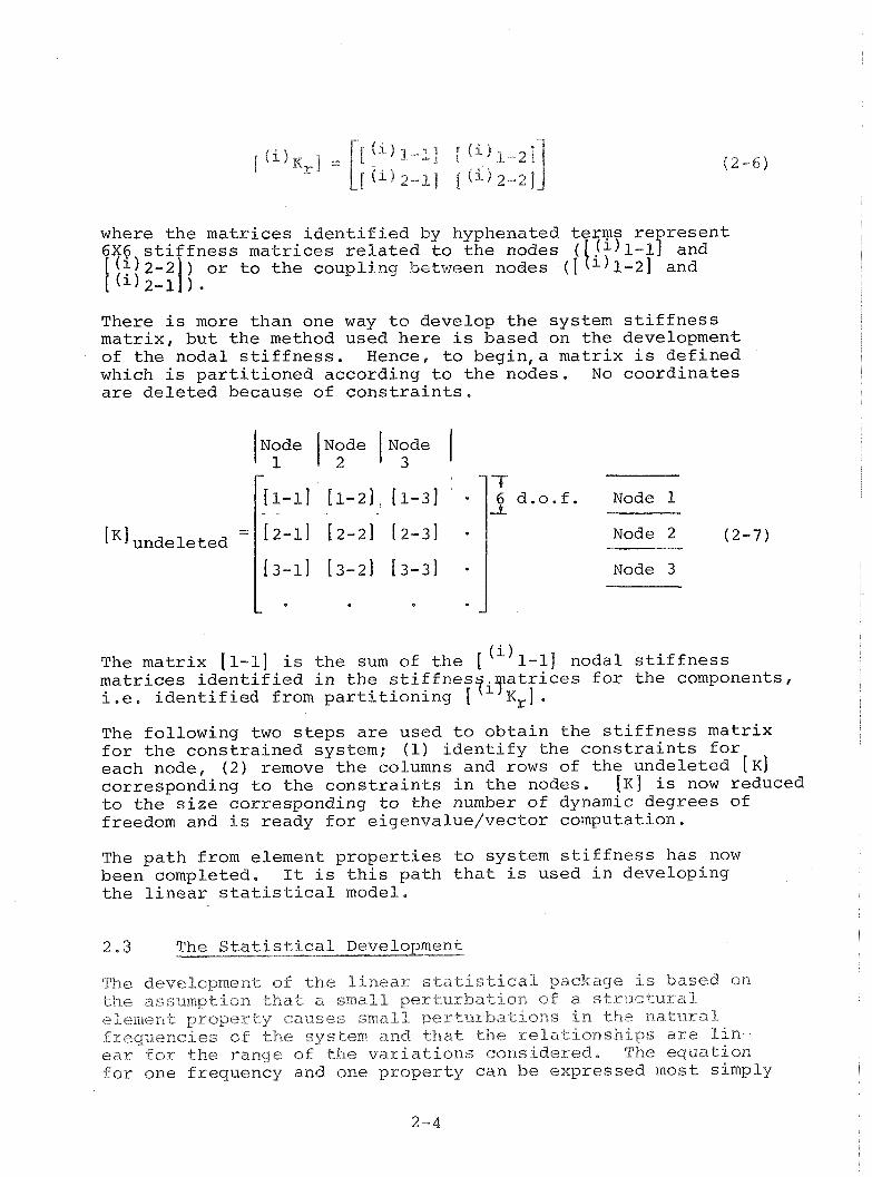
where t h e m a t r i c e s i d e n t i f i e d by hyphenated terms r e r e s e n t 6x6 s t i f f n e s s ma t r i ce s r e l a t e d t o t h e nodes ( ( i ) l - l P and [ ( $ ) 2 - 2 ) ) o r t o t h e coupl ing between nodes ( [ I i ) l - L ] and [ (") 2-11 1 . There i s more than one way t o develop t h e system s t i f f n e s s mat r ix , b u t t h e method used he re i s based on t h e development of t h e nodal s t i f f n e s s . Hence, t o b e g i n , a ma t r ix i s de f ined which i s p a r t i t i o n e d according t o t h e nodes. No coord ina t e s a r e d e l e t e d because of c o n s t r a i n t s .

Node Node Node l l 1 2 1 3 1 l{l-l] [ l - 2 1 , 11-31 - I d . 0 . f . Node 1

Node 2 (2-7)

Node 3

The ma t r ix [l-l] i s t h e sum of t h e [ ( i ) l - l~ nodal s t i f f n e s s ma t r i ce s i d e n t i f i e d i n t h e s t i f f n e s f o r t h e components, i . e . i d e n t i f i e d from p a r t i t i o n i n g [

The fol lowing two s t e p s a r e used t o o b t a i n t h e s t i f f n e s s ma t r ix f o r t h e cons t r a ined system; (1) i d e n t i f y t h e c o n s t r a i n t s f o r each node, ( 2 ) remove t h e columns and rows of t h e unde le ted [ K ] corresponding t o t h e c o n s t r a i n t s i n t h e nodes. [ K ] i s now reduced t o t h e s i z e corresponding t o t h e number of dynamic degrees of freedom and i s ready f o r e igenva lue /vec tor computation.

The p a t h from element p r o p e r t i e s t o system s t i f f n e s s has now been completed. I t i s t h i s pa th t h a t i s used i n developing t h e l i n e a r s t a t i s t i c a l model.

2 - 3 The S t a t i s t i c a l Development

The development s f t h e linear statistical package is based an the assumption that a small perturbation sf a structural element proper ty cause s small perturbations in the n a t u r a l frequencies of the system and that the relationships are linear for the range of t h e variations cons idered , The equa t ion f o r one frequency and one p rope r ty can be expressed most simply

2 - 3 - The S"ca4-isticd -------- ~ l ) c v e l o p m e n t ( ~ o n t ' d )

where w is a single frequency and p is some property of some element in the system. The term, aw/ap, is composed of all of the modifications to p which take place when tracing through the system from the property, through the elemental stiffness matrix, through a rotation, through a compatibility matrix and finally through the eigenvalue computation. We can show this symbolically in a series of partial derivatives

The dependence of an eigenvalue upon the variation of an element in the stiffness

matrix

The first two partial derivatives were developed in Reference (1). They are

and

where k is the pqth element in the system stiffness matrix, I?q and X p i and x q i are the pth and yth elements in the ith eigen- vec to r ,

Similar expressions were derived for 2Xi , ax.^, and axji 3 -- - '"~4 a k ~ q

a m Pq

although the expressions concerning the eigenvector components a r e r ede r ived i n a more convenient form i n Sec t ion 3 of t h i s r e p o r t .

Of t h e p a r t i a l d e r i v a t i v e exp res s ions shown i n (2 -9 ) , a l l b u t t h e f i r s t a r e ma t r i ce s o r v e c t o r s r a t h e r t han s c a l a r s ; and i f t h e number of f r equenc ie s and e lementa l p r o p e r t i e s a r e in - c r eased and i f modes a r e cons idered , a l l become nonsca la r ( i . e . ma t r ix ) express ions . A t t h i s p o i n t , we w i l l a t t empt t o d e f i n e each of t h e s e exp res s ions more e x a c t l y s t a r t i n g wi th t h e p h y s i c a l p r o p e r t i e s and working t o t h e system s t i f f n e s s mat r ix .

Using a beam element such a s t h a t d i s cus sed i n Sec t ion 2 .2 , develop a v e c t o r of t h e p h y s i c a l p r o p e r t i e s . These p r o p e r t i e s would normally be inc luded i n t h e program i n p u t d a t a .

By p e r t u r b i n g each of t h e p r o p e r t i e s , l i n e a r express ions can be w r i t t e n f o r r e l a t i n g t h e components of t h e e lementa l s t i f f - ness m a t r i x t o t h e p r o p e r t i e s . The exp res s ions can be p u t i n t o t h e fol lowing ma t r ix form:

It is, however, more convenient to keep the p a r t i a l derivatives, akij -- , in a matrix form until the stiffness elements have been ~ P R rotated into system or global coordinates, Hence the stiffness matrix is differentiated n times, once for each property which can vary, There are now n matrices of partial derivatives as shown

below con ta in ing a l l t he sensitivities sf the stiffness elements to the properties

i, a ( k ) . a *

i, a (k )

ap2 i f a ~ n

To p u t t h e s e p a r t i a l d e r i v a t i v e s i n t o sys tem c o o r d i n a t e s p r e and p o s t m u l t i p l y t h e s e m a t r i c e s by t h e r o t a t i o n m a t r i x

[ ( i ) ~ ] f o r e lement i .

- - r i ) R ] Ii) 3 ( k ) ] F i ) R ] '

a p 1

I ~ ) R ] L") a ( k ) ] [ ( ~ ) R ] I

ap2

The e lements of e tc . can now be removed and

p l a c e d i n t o columns w i t h e a c h column r e p r e s e n t i n g a dependency upon a d i f f e r e n t p r o p e r t y , p .

a m -

- - *

N o t e that a (k) --- i s a matrix of n columns representing the

I a c p ~ J n properties and rn raws representing the rn elements in

This matrix (Equation (2-15)) encom partial derivatives shown in Equation ( 2 - 9 ) ,

The components of the matrix with-

1 a P J in the computer program because they are based on the same fixed expressions used to develop the stiffness matrix.

This generally covers the development of partial derivatives re- lating changes in physical properties to changes in modal characteristics. One additional point is worth mentioning, however. In developing the partial derivatives ahi and axji, note that not

- a k ~ q a k ~ q

all of the partial derivatives are required; only those with respect to system stiffness elements krs which correspond to elements (i 1 k,, in the rotated elemental stiffness matrix. Hence, logic

13

must be introduced into the program to compute only chose partial derivatives which relate to structural element i. We can denote this consideration for element i by introducing the presuperscript (i) into the matrix expression

The expression in Equation (2 . 9 ) can be written as a product of a series of matrices (it is convenient to work with dX rather than dw; results can be put in terms of w in the final operation).

and

* The development here is for stiffness uncertainty alone, The method is the same for mass,and mass uncertainty is included in the VIDAP program, See Sections 4 and 5 for further details.

2-8

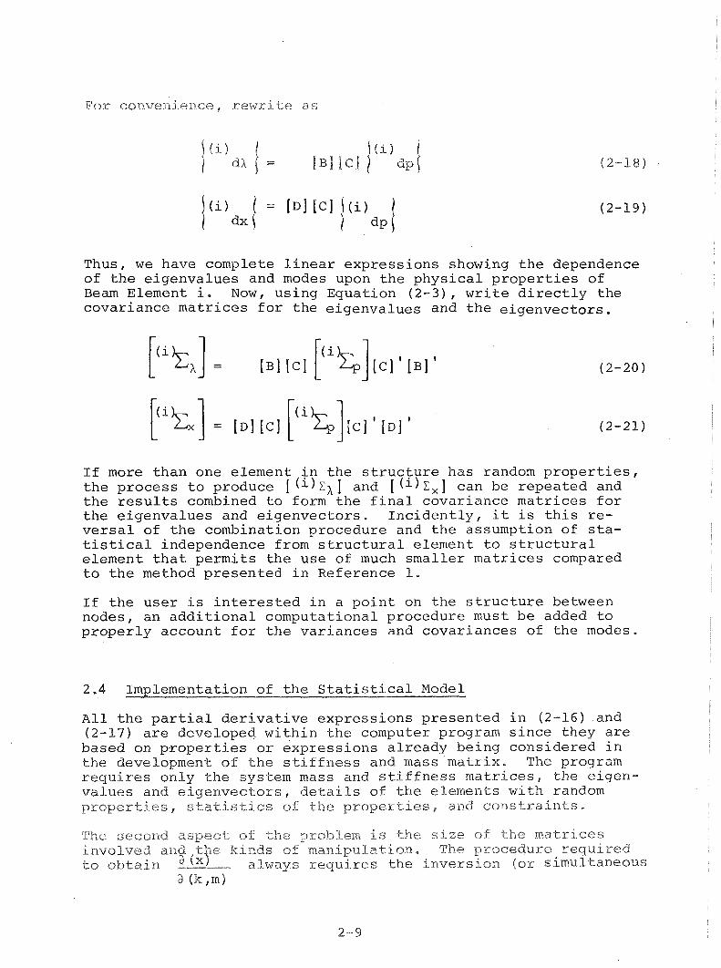
For convenience, rewrite as

Thus, we have complete linear expressions showing the dependence of the eigenvalues and modes upon the physical properties of Beam Element i. Now, using Equation (2-3), write directly the covariance matrices for the eigenvalues and the eigenvectors.

If more than one element jn the structure has random properties, the process to produce [ (l) 1, ] and [ (l) I,] can be repeated and the results combined to form the final covariance matrices for the eigenvalues and eigenvectors. Incidently, it is this re- versal of the combination procedure and the assumption of statistical independence from structural element to structural element that permits the use of much smaller matrices compared to the method presented in Reference 1.

If the user is interested in a point on the structure between nodes, an additional computational procedure must be added to properly account for the variances and covariances of the modes.

All the partial derivative expressions presented in (2-16) and (2-17) are developed within the computer program since they are based on properties or expressions already being considered in the development of the stiffness and mass matrix. The program requires only the system mass and stiffness matrices, the eigenvalues and eigenvectors, details of the elements with random properties, statistics of the properties, and constraints,

The second aspect of t h e problem i s the s i z e of the matrices involved and t e kinds of manipulation, The procedure required to obtain a (xf - always requires the inversion (or simultaneous

a (k,m)

equation solution) of (n-1) x (n-1) matrices making this the most expensive part sf the statistical computations, The other processes are primarily the development of elements by simple formulae or the multiplication of matrices, both of which are considerably cheaper t h a n inversion. Every effort has been made to minimize the matrix storage requirements by using only half of the symmetric matrices and storing in a new matrix having the number of columns corresponding to the semi-bandwidth and the number of rows corresponding to the degrees of freedom. The simultaneous equation solution for axji (to be shown in Section 3)

a k ~ q is accomplished, in part, by triangular decomposition of the matrix expression [K-X~M]. This is the fastest and most accurate method available and requires the least storage.

The output of the statistical data can be quite voluminous. For instance, in displaying the statistical parameters for all 100 eigenvectors of a 100 degree-of-freedom system, the covariance matrix has the dimensions of 10,000 x 10,000. Since the user will never have need for all of this data, he can confine the output to the specific eigenvectors and sections of the eigenvectors which are of interest.

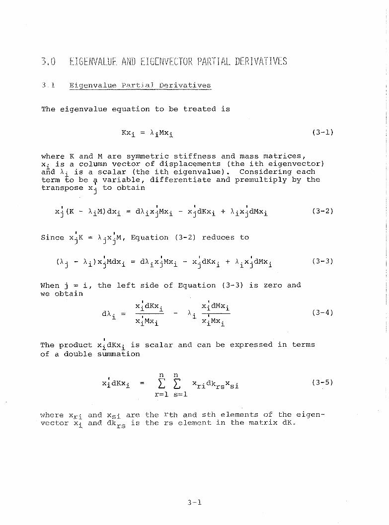
3 , 0 ElGENVALUE AND EIGENVECTOK PARTIAL DERIVATIVES

3 - 1 Eigenvalue Partial Derivatives

The e igenva lue equa t ion t o be t r e a t e d i s

where K and M a r e symmetric s t i f f n e s s and mass m a t r i c e s , xi i s a column v e c t o r of d isplacements ( t h e i t h e igenvec to r ) and A i i s a s c a l a r ( t h e i t h e igenva lue ) . Consider ing each term t o be 9 v a r i a b l e , d i f f e r e n t i a t e and premul t ip ly by t h e t ranspose x t o o b t a i n

j

t

Since x .K = X X ~ M , Equation (3 -2 ) reduces t o I 3 3

When j = i , t h e l e f t s i d e of Equation (3-3) i s zero and w e o b t a i n

I

The produc t xidKxi is s c a l a r and can be expressed i n terms of a double summation

where x,i and X s i a r e the rth and sth elements of the eigenvector xi and dk,, is the rs element i n the mat r ix d K .

1

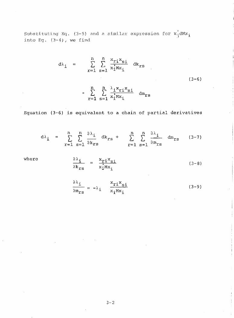
Substituting E q , ( 3 - 5 ) and a similar expression f o r x . m x i J

into Eq, (3-43 , we find

Equation (3-6) i s e q u i v a l e n t t o a cha in of p a r t i a l d e r i v a t i v e s

where

3 , 2 Eigenveetor Partial Derivatives ---

Differentiate Eg, (3-1) ,

and s u b s t i t u t e E q . (3-4) f o r dXi

Choose f o r example a dependence upon s t i f f n e s s element krs. Then

where t h e exp res s ion xSi{bjr} i s equ iva l en t t o a ze ro v e c t o r w i th a non-zero e lement , x s i , i n t h e r t h row. 6 j r i s a Kronecker d e l t a de f ined by

j r e p r e s e n t s t h e number of t h e row o r element i n t h e v e c t o r i n t h i s ca se .

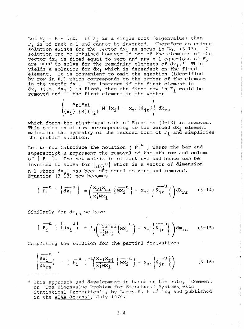
L e t Fi =I K - XiM, I f Ai is a s i n g l e roo t (e igenva lue) t h e n F i i s of rank n-1 and cannot be i n v e r t e d , Therefore no unique s o l u t i o n e x i s t s f o r t h e v e c t o r dxi as shown i n E q . (3-13) . A s o l u t i o n can be ob ta ined however i f one of t h e elements s f t h e v e c t o r dxi i s f i x e d equa l t o ze ro and any n-1 equa t ions of F i a r e used t o s o l v e f o r t h e remaining e lements of dxi.* This y i e l d s a s o l u t i o n f o r dxi which i s dependent on t h e f i x e d e lement . I t i s convenient t o omit t h e equa t ion ( i d e n t i f i e d by row i n Fi) which corresponds t o t h e number of t h e element i n t h e v e c t o r dxi. For i n s t a n c e i f t h e f i r s t element i n dxi ( i . e . dxli) 1s f i x e d , t hen t h e f i r s t row i n Fi would be removed and t h e f i r s t element i n t h e v e c t o r

which forms t h e r ight-hand s i d e of Equation (3-13) i s removed. This omission o f row corresponding t o t h e zeroed dx. element main ta ins t h e symmetry of t h e reduced form of F i an& s i m p l i f i e s t h e problem s o l u t i o n .

-u Let us now in t roduce t h e n o t a t i o n f F i ] where t h e b a r and s u p e r s c r i p t u r e p r e s e n t t h e removal of t h e u th row and column of [ Fi 1 . The new ma t r ix i s of rank n-1 and hence can be i n v e r t e d t o s o l v e f o r ldFiu) which i s a vec to r of dimension n-1 where dxui has been s e t equa l t o ze ro and removed. Equation (3-13) now becomes

S i m i l a r l y f o r dmrs we have

Completing t h e s o l u t i o n f o r t h e p a r t i a l d e r i v a t i v e s

* This approach and development is based on t h e n o t e , ""Coment on "The Eigenvalue Problem fo r Structural Systems with S t a t i s t i c a l P r o p e r t i e s i ' \ by L a r r y A , ~ i e f l i n g and published i n t h e AIAA J o u r n a l , J u l y 1 9 7 0 .

- U - -U. axi axi

and =z -hi am,, a k r s

Numerically it i s n o t necessary t o i n v e r t qU] since Equation (3-16) can be so lved a s a s e t of simultaneous a l g e b r a i c equa t ions .

A d i s cus s ion of t h e ma t r ix decomposition procedure s e l e c t e d t o

The e igenvec tor p a r t i a l d e r i v a t i v e s i n Equation (3-16) a r e n o t t r u l y r e p r e s e n t a t i v e of any system un le s s a r e s t r i c t i o n has been placed upon t h e e igenvec to r s t h a t t h e element xui of each e igenvec to r xi be he ld c o n s t a n t . I n i n s t a n c e s where t h e e igenvec to r s a r e normalized such t h a t t h e f i r s t element i s always one, Equa- t i o n (3-16) would be v a l i d f o r t h e s u p e r s c r i p t u equa l t o one.

axli = 0 and x = c o n s t a n t . I f , however, That i s t o s ay , - li a k r s

t h e e igenvec tor s o l u t i o n r e q u i r e s a c o n s t a n t gene ra l i zed mass (xiMxi = cons t . ) , Equation (3-16) i s no t s a t i s f a c t o r y and a f u r t h e r o p e r a t i o n i s necessary t o o b t a i n t h e f u l l vec to r of

p a r t i a l d e r i v a t i v e s ,

Define (,<\ a s t h e v e c t o r of p a r t i a l d e r i v a t i v e s

I! akrs developed from (3-16) b u t wi th a zero i n s e r t e d i n t h e u t h element r a t h e r than having t h e u t h element omi t ted . That i s

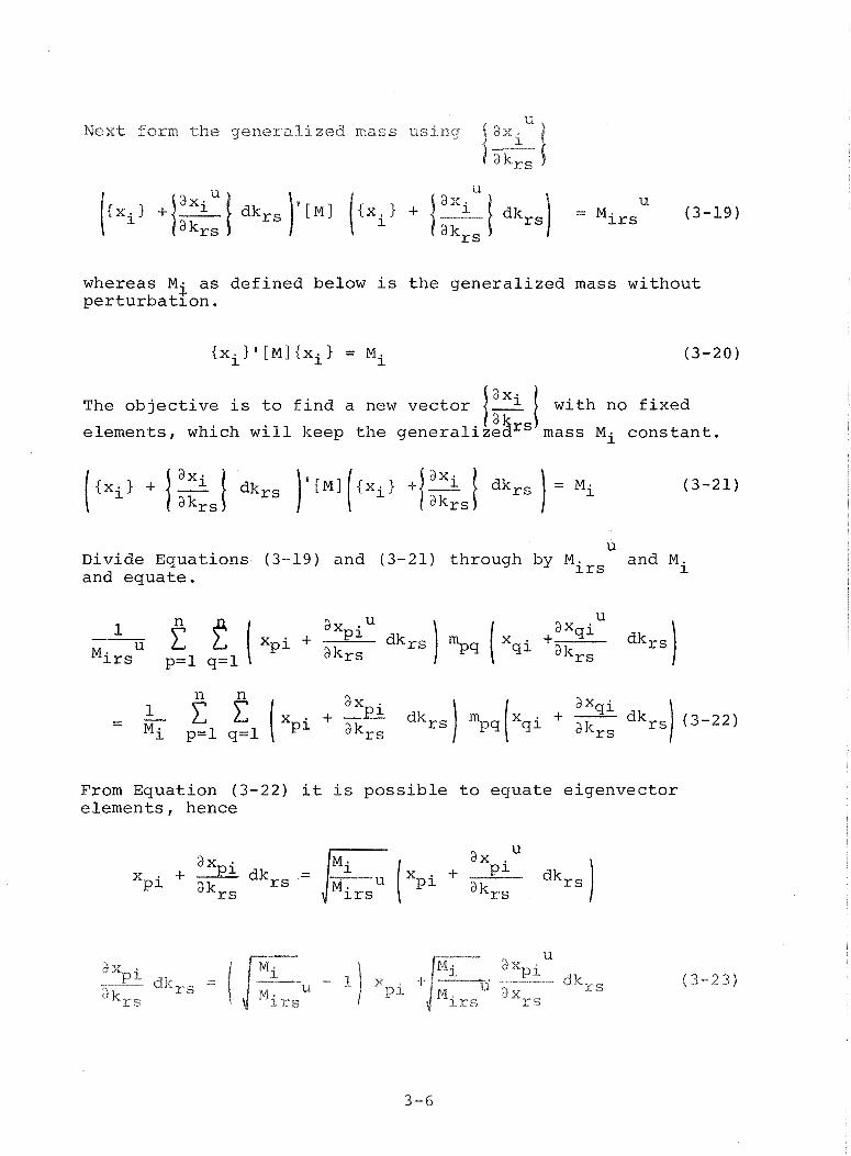
Next form the generalized mass using

u - u

dkr s - (3-19)

whereas M i a s d e f i n e d below i s t h e g e n e r a l i z e d mass w i thou t p e r t u r b a t i o n .

The o b j e c t i v e i s t o f i n d a new v e c t o r 1 w i th no f i x e d

e lements , which w i l l keep t h e gene ra l i z ed rS mass Mi c o n s t a n t .

u Divide Equat ions (3-19) and (3-21) through by Mirs and Mi and equa t e .

From Equat ion (3-22) it i s p o s s i b l e t o equa t e e igenvec to r e l emen t s , hence

The r a t i o contains t h e derivative dkr,, Multiplying

U o u t Mi,, from Equa t ion ( 3 - 1 9 1 , we have

2 Note t h a t [ M I is symmet r i ca l and (dk,,) << dk,,. E q u a t i o n (3-24) becomes

Then

1 u 1

1 + M i i " " - j M ~ { ~ ~ i d k ~ ~ a k r s

which expands i n t o

+ - 'a (2 1 % ( I [ M I ixi}dkrs 2.4 Mi ak,,

2 Again assume (dk,,) << dkrs, c a u s i n g the higher o r d e r terms af ( 3 - 2 7 ) t o v a n i s h ,

Next, s u b s t i t u t e this l i n e a r i z e d f o r m of (3-27) i n t o ( 3 - 2 3 ) t o get

and

Note i n Equa t ion ( 3 - 2 9 ) t h a t axpi i s n o t symmet r i ca l , i . e .

a x p i ax a k r s - *A* a k r s a k s r T h i s means t h a t t h e p r o p e r t y of symmetry which i s s o c o n v e n i e n t i n t h e h a n d l i n g o f t h e mass and s t i f f n e s s m a t r i c e s i s l o s t and t h e p a r t i a l d e r i v a t i v e s o f x p i must be computed w i t h r e s p e c t t o e v e r y e lement o f t h e s t i f f n e s s m a t r i x . However, s i n c e t h e s t i f f n e s s m a t r i x w i l l a lways be symmet r i ca l , t h e r e i s no r e a s o n t o t r e a t t h e p a r t i a l d e r i v a t i v e s f o r symmet r i ca l e l ements s e p a r - a t e l y . Thus add t h e two and t r e a t t h e sum. Using Equa t ion ( 3 - 1 6 ) ,

Equation ( 3 - 3 0 ) is very similar to (3 -16) except for the factor of 2 and the additional element,

ELEMENT PROPERTY SENSITIVITY MATRX CES

The s t r u c t u r a l makeup of a g r e a t many s t r u c t u r e s can be descr ibed by a s e r i e s of beam and p l a t e f i n i t e e lements . I n t h i s s tudy , a s t anda rd beam element (12 degrees of freedom) and a t r i a n g u l a r p l a t e element (15 degrees of freedom) w e r e used i n developing t h e r e l a t i o n s h i p between p h y s i c a l pro- p e r t i e s of t h e s t r u c t u r e and t h e e igenva lues and e igenvec to r s of t h e dynamic system. I n a d d i t i o n , procedures a r e descr ibed and al lowances a r e made f o r t h e i n c l u s i o n of s t i f f n e s s ma t r i ce s f o r o t h e r element-types.

The procedure used f o r t h e development of t h e s t i f f n e s s ma t r ix p a r t i a l d e r i v a t i v e s i s summarized a s fo l lows:

(1) t h e s t i f f n e s s mat r ix i s i d e n t i f i e d f o r t h e s t r u c t u r a l element of i n t e r e s t i n l o c a l (element) coo rd ina t e s

( 2 ) v a r i a b l e s i n t h e s t i f f n e s s ma t r ix which can be random v a r i a b l e s a r e i d e n t i f i e d (no te s t r u c t u r a l geometry such a s l o c a t i o n s of nodes a r e n o t considered t o be random).

( 3 ) t h e s t i f f n e s s ma t r ix i s d i f f e r e n t i a t e d wi th r e s p e c t t o each of t h e p r o p e r t i e s which can be random. Each s e t of p a r t i a l d e r i v a t i v e s (wi th r e s p e c t t o a p rope r ty ) i s s t o r e d i n a s e p a r a t e mat r ix .

( 4 ) r o t a t i o n ma t r i ce s a r e developed from t h e coor- d i n a t e s of t h e nodes.

( 5 ) t h e ma t r i ce s of p a r t i a l d e r i v a t i v e s i n l o c a l (e lement) coo rd ina t e s a r e transformed i n t o

ma t r i ce s of p a r t i a l d e r i v a t i v e s i n system ( g l o b a l ) coo rd ina t e s .

( 6 ) t h e p a r t i a l d e r i v a t i v e s from each of t h e ma t r i ce s a r e removed and p u t i n columnar form i n a new mat r ix . Each column r e p r e s e n t s s e n s i t i v i t i e s of s t i f f n e s s elements t o a d i f f e r e n t p h y s i c a l p rope r ty .

The procedure a s desc r ibed i s used on both t h e beam and p l a t e e lements i n t h e s e c t i o n s t h a t fol low.

4-1 B e a m Element

4,1,1 In t roduc t ion

The beam element s t i f f n e s s p rope r ty s e n s i t i v i t y m a t r i c e s wi th r e s p e c t t o a g l o b a l coo rd ina t e system a r e developed i n t h i s s e c t i o n . The end r e s u l t i s a p roper ty s e n s i t i v i t y ma t r ix which r e l a t e s t h e p a r t i a l d e r i v a t i v e s of member geometr ic and m a t e r i a l p r o p e r t i e s t o t h e p a r t i a l d e r i v a t i v e s of each element i n t h e beam s t i f f n e s s mat r ix .

The beam element i s assumed t o be s t r a i g h t and have a un i - form c r o s s s e c t i o n . M a t e r i a l p r o p e r t i e s a r e i n v a r i a n t a long t h e e l emen t ' s l e n g t h and bo th i n t e r n a l shea r and bending deformat ions a r e cons idered . Each c ros s - sec t ion i s capable of r e s i s t i n g a x i a l and shear ing f o r c e s , bending moments about t h e two p r i n c i p a l axes i n t h e p lane of t h e c r o s s - s e c t i o n , and a t w i s t i n g moment about t h e c e n t r o i d a l a x i s . F igure 4 - 1 shows a t y p i c a l beam element wi th axes Ym and Zm corresponding t o t h e p r i n c i p a l axes of t h e c ros s - s e c t i o n and t h e c e n t r o i d a l a x i s , Xm. The s i x independent displacements a t each end of t h e element a r e shown i n t h i s f i g u r e and noted a s type ( u ) d isplacements .

I t i s impor tan t t o emphasize two p o i n t s . F i r s t , t h e member c e n t r o i d a l a x i s , Xm, i s always d i r e c t e d along t h e l eng th of t h e element and corresponds t o t h e bending n e u t r a l a x i s of t h e beam. Second, t h e Ym and Zm axes a r e i d e n t i c a l wi th t h e two p r i n c i p a l axes of t h e beam c ros s - sec t ion . The importance of t h i s i s t h e uncoupling of t h e induced s t r e s s e s caused by t h e bending moments corresponding t o Us, U g , U 1 1 and U 1 2 ( s e e Reference 3 , Page 7 0 ) .

4 . 1 . 2 Beam S t i f f n e s s Proper ty S e n s i t i v i t y Matrix

The d e r i v a t i o n of t h e beam s t i f f n e s s mat r ix f o r t h e g e n e r a l beam element shown i n F igure 4 - 1 can be r e a d i l y a v a i l a b l e i n a number of r e f e r e n c e s ( e . g . , s e e Ref. 3 , pgs. 7 0 - 8 2 ) . Table 4 - 1 g i v e s t h e r e s u l t i n g member s t i f f n e s s ma t r ix which was de r ived inc lud ing shea r and bending deformat ions . The beam p r o p e r t i e s t h a t a r e p r e s e n t i n t h i s ma t r ix , and t h e ones t h a t may be considered a s random v a r i a b l e s a r e :

F i g u r e 4 - 1 Genera l Beam F i n i t e Element

E - Young" modulus of e l a s t i c i t y

v - Poisson" Ratio

A - Beam c r o s s - s e c t i o n a l a r e a

12, I3 - Beam c r o s s - s e c t i o n a l moment of i n e r t i a a b o u t Ym and Zm a x e s , r e s p e c t i v e l y .

J - Beam c r o s s - s e c t i o n a l p o l a r moment o f i n e r t i a abou t X , a x i s .

SF3, SF2 - Beam c r o s s - s e c t i o n a l s h e a r f a c t o r s a b o u t t h e Ym and Zm a x e s , r e s p e c t i v e l y .

I t i s no ted t h a t t h e p r o p e r t i e s which i n v o l v e t h e g e o m e t r i c d imensions of t h e c r o s s s e c t i o n a r e n o t independen t random v a r i a b l e s . I n g e n e r a l , t h e c o v a r i a n c e s between t h e s e p ro - p e r t i e s are non-zero and f o r e a c h d i s t i n c t c r o s s - s e c t i o n ( e . g , c i r c u l a r , s q u a r e , t u b u l a r , e t c . ) t h e r e e x i s t s a unique r e l a t i o n s h i p between t h e c r o s s - s e c t i o n d imens iona l s t a t i s t i c s and t h e above mentioned p r o p e r t y s t a t i s t i c s . T h i s t o p i c i s d i s c u s s e d i n d e t a i l i n S e c t i o n 5 .

C e n t r a l t o t h e f o r m u l a t i o n of t h e n a t u r a l f r equency and modal s t a t i s t i c s of a s t r u c t u r e i s t h e p r o p e r t y s e n s i t i v i t y m a t r i x . T h i s m a t r i x m a t h e m a t i c a l l y r e l a t e s l i n e a r v a r i a t i o n s i n t h e beam random p r o p e r t i e s t o t h e fo rce -d i sp lacement r e l a - t i o n s h i p ( i .e . s t i f f n e s s m a t r i x ) . Corresponding t o e a c h beam p r o p e r t y t h e r e i s a unique p r o p e r t y s e n s i t i v i t y m a t r i x , n o t e d

where

E K ~ ~ ~ ~ ] = beam s t i f f n e s s m a t r i x i n t h e Xm, Y,, Zm c o o r d i n a t e sys tem

These e i g h t s e n s i t i v i t y m a t r i c e s a r e a l l of o r d e r 1 2 x 12 and e a c h r e s u l t s from t a k i n g t h e p a r t i a l d e r i v a t i v e of each e lement i n t h e s t i f f n e s s m a t r i x w i t h r e s p e c t t o a p r e s c r i b e d p r o p e r t y . For example,

a LKbearn]

is a 12 x 12 property s e n s i t i v i t y ma t r ix c a l c u l a t e d by taking

the partial derivative of each element in [ K ~ ~ ~ ~ ] with respect to J= Since only the elements in the f o u r t h rows and co lmns contain J (Table 4 - P ) all other elements in the sensitivity matrix are zero. Therefore, the property sensitivity matrix corresponding to the torsional constant has only four non-zero e lements - (4,4), (4,10), (E0,4) and (PO, 10). The o t h e r seven s e n s i t i v i t y ma t r i ce s a r e , i n g e n e r a l , more complicated, b u t t h e method of development i s t h e same.

C e r t a i n c h a r a c t e r i s t i c s of t h e s e p rope r ty s e n s i t i v i t y ma t r i ce s a r e worth no t ing . F i r s t , t hey a r e symmetric m a t r i c e s because they a r e ob ta ined by p a r t i a l d i f f e r e n t i a t i o n of t h e symmetric s t i f f n e s s ma t r ix . Second, they a r e n o t n e c e s s a r i l y p o s i t i v e d e f i n i t e . This fo l lows from observ ing t h a t t h e t e r m s on t h e d iagona l of t h e p rope r ty s e n s i t i v i t y ma t r i ce s may be ze ro o r nega t ive .

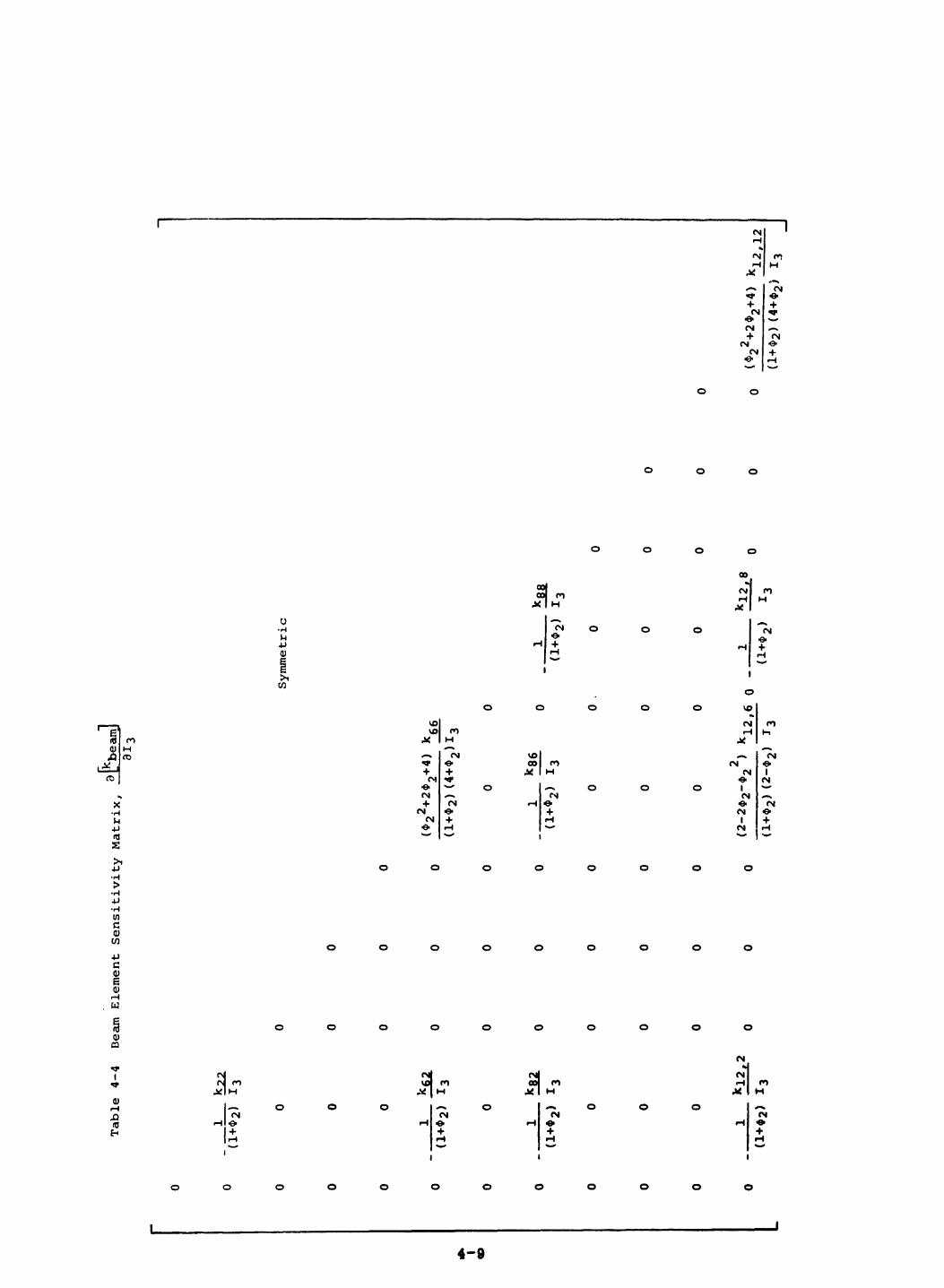
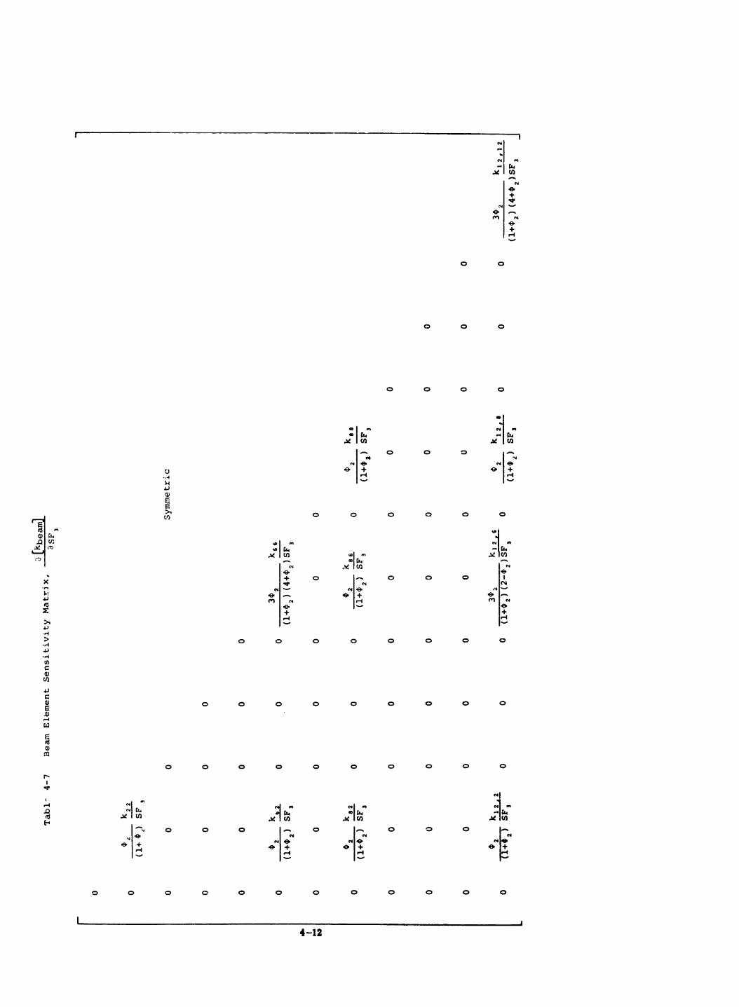
Seven of t h e e i g h t s e n s i t i v i t y m a t r i c e s a r e shown i n t h e fol lowing t a b l e s (Table 4-2 t o 4 - 8 ) . The e lements a r e shown a s a f a c t o r t i m e s t h e o r i g i n a l s t i f f n e s s e lement , e .g.

The t a b l e f o r a[Kbeam] i s omi t ted because it i s e q u i v a l e n t a E

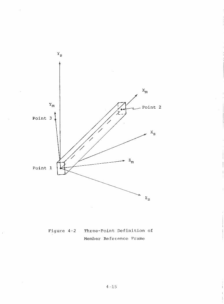
*woTqaas-ssoxa mGaq ayq $0 saxp xediauy~d ayq so auo pue srxe weaq ayq Aq pamxaz auegd e u~ sag A~~eu~sw qvrod

"s~xc ayq 07 anTqeTax ws~qaas-ssox~ ayq quaTxo aq. pasn ST

pue srxe laquarn ay7 uoxg APAP pauyzap aq qsnu qu~od pqyq ay& "JaW3m aq7 go pua ysea %e pa3eao-I *s~xe qeproxquaa weaq

ayq uo axe squ~od ayq $0 OM& (z-$ axnbrd) uoTqeqox sly3 aur3ap oq papaau axe a~eds u~ squ~od 7surqsTp aaxya 'amex3

"A "x ayq 03 amexj m~ "x ayq moxj uoyqemxojsuexq aqPUTPx003 ayq bu~quasaxdax xyxqgm E x E e s~ [hi axayM

[~1[01[01[01

(1-v) [~1[01[01 [A1[01

= [XI

[ A1

un03 ayq spy [a] '[a] 'xrxqem uoyqeqox e u? pauyequoa xayqo ayq oq

amex3 aauaxa3ax auo moxj suorqeqox qauyqsyp aaxyq 30 aauanbas e Aq paysy~dmoaae ST srya *amex3 aauaxa~ax maqsAs ayq

oq qaadsax yqy~ paysTTqeqsa sy amex3 aauaxa3ax xaqmam ayq 30 uoyqequarlo ayq 'qsxy~ *xyxqem ssauggyqs buypuodsaxxoa ayq 30

uoyqeqox ayq s~a11exed amex3 aauaxajax ~eqo1b e 07 xaqmam e mox3 xyxqem Aqr~~qysuas Aqxadoxd xaqmam ayq 30 uoyqeqox ayz

'uoyqaas syyq ur paquasaxd axe yseq s~yq oq queaaTax sda7.s TPuoTqTPPe ayq ATUO "(TE - 87: sabed ' paauaxa3aa

aas *bWa) axayMas1a pun03 aq uea saayxqem quamaae~dsyp pup aax03 30 uoyqeqox ayq 203 suoyqenba 30 uoyqeAyxap paTyeqaa

'aurexj aauaragax '~eqo1b xo ImaqsAs ayq oquy uoyqeqox sq? ssnasyp am uoyqaas syyq UI * ("z lWx) amex3 aauaxajax

xaqmam ayq oq qaadsax yqyM pado~anap sy xyxqem Aqynyqysuas Aqzadoxd ureaq ayq 'uoyqaas snoynaxd ayq uy paqyxasap se 'qsx-rd

'saayxqem Aqynyqysuas Aqxadoxd xaqmam ayq 30 quamdo~anap ayq uy paMoTTo3 sy axnpaaoxd uoyqeqox e yans *(S~ 1s~ 'Sx)

amex3 aauaxagax axnqanxqs ayq uy suoyssaxdxa bu-rpuodsaxxoa oq sayqxadoxd ayq aqeqox A~~ea~qemaqsAs oq uayq pup ("2 lux)

awl3 aauaxagax xaqmam ayq 30 smxaq uy xaqmam xe-payqxed e 203 sayqxadoxd ssau33yqs pue Tepqxauy 11-e auygap qsxyc 07

sma~qoxd axnqanxqs xyxqem uy quayua~uoa sy 71 Oxaqmam ayq 30 saxe pdyauyxd 1euoyqaas-ssoxs o~q ayq pue syxe Tepyoxquaa

ayq 07 puodsaxxoa "z puue "A dsaxe asayq maxqoxd xno u? pue (1-p axn6yd aas *boa) xaqmam Texnqanxqs xe1nayqxed ayq

oq wadsax yqyM paurzap ST amex3 syyq 30 saxe ayq 30 uoyq -equayxo ayg *amex3 aauaxasax xaqmam ayq sy adAq puoaas ay&

-aaeds pyq.xauT u~ paxrs aq 02 pamsse sr ya~y~ amex2 aaua --xagax maqsAs xo ~eqo%h ayq sy qsz~j aya ~rna~qazd s~ymeuAp

Xexnqanxqs e ur pssn Apaensn axxi? sauxexj aarraxagax so sadAq OM&

saayxqeM dqsn~qrsua~ Wq~adaxd mesa ayq so uof%-eqox caa"$

P o i n t

P o i n t

F i g u r e 4-2 T h r e e - P o i n t D e f i n i t i o n o f

Member R e f e r e n c e Frame

The coordinate n m b e r i n g of t h e beam stiffness m a t r i x (node 1: 3 transl= 3 rot, ; node 2: 3 transl, , 3 rot, ) and t h e straight cen t ro ida l axis s f the beam permit the r e p e a t e d use of [ y ] consecutiveby down the diagonal of [I?],

The m a t r i x e q u a t i o n d e f i n i n g t h e n e c e s s a r y r o t a t i o n o p e r a t i o n s i s

Once a l l o f t h e e lements of [3'::j beam have been computed, t h e y a r e s t o r e d i n a s i n g l e column i n a new m a t r i x of t h e form shown i n Equat ion ( 2 - 1 6 ) .

The form o f ( 4 - 3 ) .

t h i s m a t r i x , f o r t h e beam, i s shown i n Equa t ion

is syrmetrieal, o n l y elements on the

e side of the diaqona l need to be s tored

in forming

4-16

4 , 1 , 4 Beam Mass P r o p e r t y S e n s i t i v i t y Mat r ix

The mass i n t h i s a n a l y s i s i s c o n c e n t r a t e d a t t h e nodes . Hence t h e sys tem mass m a t r i x i s d i a g o n a l and each e lement a long t h e d i a g o n a l r e p r e s e n t s t h e mass o r i n e r t i a c o r r e s p o n d i n g t o a dynamic d e g r e e of freedom. The masses and i n e r t i a s a r e i n p u t i n sys tem c o o r d i n a t e s and t h e r e f o r e t h e component mass m a t r i x i s n o t r o t a t e d a s i s t h e component s t i f f n e s s m a t r i x .

The mass a t t h e node i s treated a s t h e random v a r i a b l e . S i n c e t h e mass i n t h e t h r e e t r a n s l a t i o n a l d i r e c t i o n s i s by d e f i n i t i o n t h e same, t h e t r a n s f o r m a t i o n i s u n i t y . For t h e t h r e e r o t a t i o n a l d e g r e e s of freedom t h e mass i s a f a c t o r i n t h e moment of i n e r t i a a b o u t e a c h of t h e t h r e e a x e s , t h u s

Looking a t t h e beam e lement w e have two nodes w i t h t h e mass d i s t r i b u t e d e q u a l l y a t b o t h ends . The u n c o n s t r a i n e d mass m a t r i x f o r s t r u c t u r a l e l ement (i) i n sys tem c o o r d i n a t e s i s

Elements m , , , m2,, m , , , m , , , m , , , and m , , a r e a l l e q u a l and e a c h e q u a l h a l f t h e t o t a l beam mass. Elements m 1 4 , m S 5 , m , , , , , ,

m 1 1 , 1 1 a r e e q u a l and e q u i v a l e n t t o some s p e c i f i e d moment of i n e r t i a a b o u t t h e X,, Y, axes a t e a c h end of t h e beam, Elements

m,, and m 1 2 , 1 2 a r e e q u a l and e q u i v a l e n t t o a s p e c i f i e d moment of i n e r t i a a b o u t t h e Z, a x e s a t e a c h end , These i n e r t i a s generally con t r ibu te v e r y l i t t l e to 'the dynamic cilarae:"r.el-is-lzies of the system and i n many s t r u c t u r a l dynamic programs are set

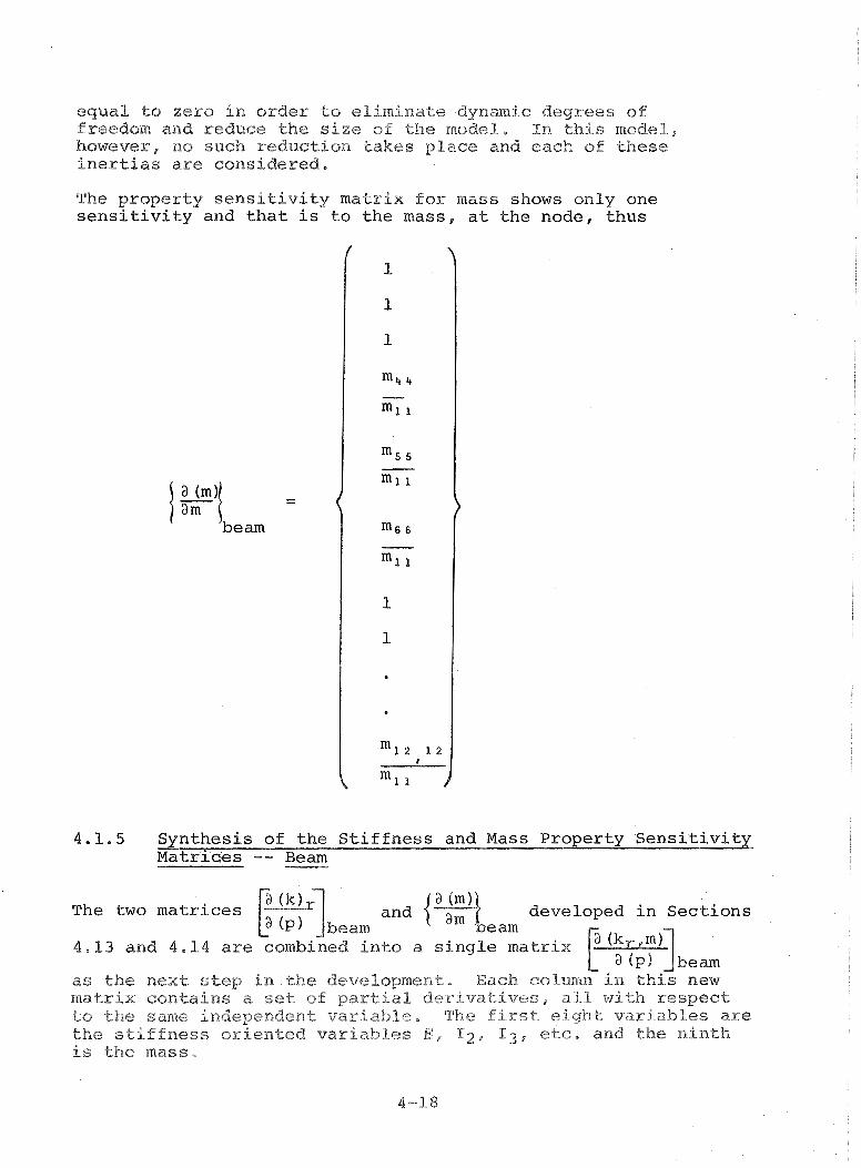
equal t o z e r o i n order t o eliminate dynmic degrees of freedom and reduce t h e s i z e s f the model, In this model, however, no such reduct ion takes place and each sf these i n e r t i a s are cons idered ,

The p rope r ty s e n s i t i v i t y ma t r ix f o r m a s s shows only one s e n s i t i v i t y and t h a t i s t o t h e mass, a t t h e node, t hus

1 ) beam

4.1.5 Matr ices -- Beam

The two m a t r i c e s and developed i n Sec t ions e a m

4 - 1 3 and 4 - 1 4 a r e n t o a s i n g l e mat r ix

as the next s t ep in the development, Each colvnlrr i n t h i s n e w matrix contains a set s f partial derivatives, a11 w i t h respect to the same independent variable, The f i r s t e ight variables are t h e stiffness oriented var iab les E , 1 2 , 1 3 , e t c , and t h e n i n t h i s the m a s s ,

The matrix is p a r t i t i o n e d as shown below,

78 rows

t up t o 1 2 rows v -

The ma t r ix w i l l always have n i n e columns b u t t h e number of rows w i l l depend upon t h e c o n s t r a i n t s upon t h e beam element. I f t h e r e a r e no c o n s t r a i n t s t h e number of rows i n each column of s t i f f n e s s p a r t i a l s w i l l be 1 /2(n2 + n) = 78 where n , t h e number of uncons t ra ined degrees of freedom i n t h i s c a s e , i s equa l t o 12. I n a d d i t i o n t h e r e w i l l be 1 2 mass p a r t i a l d e r i - v a t i v e s (one f o r each uncons t ra ined degree of freedom) making t h e t o t a l of t h e number of rows reach 90. This 90 x 9 m a t r i x i s e q u i v a l e n t t o t h e ma t r ix , LC], i n Equations (2-20) and (2-21). The number of columns must be conformable t o t h e p rope r ty covar iance mat r ix t o be developed i n Sec t ion 5 and t h e number of rows must be conformable t o t h e e igenvec tor and e igenva lue p a r t i a l d e r i v a t i v e ma t r ix which w i l l be d i scus sed f u r t h e r i n Sec t ion 6 .

The o r d e r of t h e p r o p e r t i e s a c t i n g a s independent v a r i a b l e s i n t h e p a r t i a l d e r i v a t i v e s i n each of t h e columns, moving from l e f t t o r i g h t is : E , A f 1 2 , 1 3 , V , SFZ, SF3, J, and

4 - 2 Pla te E l e m e n t

4,2,1 In t roduc t ion

The p l a t e element used i n t h i s program i s a combination of a sandwich element developed by H.C. Mart in i n 1967 (Ref. 5 ) and a t r i a n g u l a r element which r e s i s t s in-plane f o r c e s (Ref. 3 ) . The sandwich c o n s t r u c t i o n r e s i s t s both bending and shea r . This p a r t i c u l a r p l a t e was s e l e c t e d because of i t s o p e r a t i o n a l s t a t u s i n t h e STARDYNE s t r u c t u r a l dynamics program. (VIDAP was designed t o be d i r e c t l y com- p a t i b l e w i th STARDYNE.)

The procedure f o r developing t h e p l a t e p rope r ty s e n s i t i v i t y ma t r ix i s s i m i l a r t o t h a t f o r t h e beam excep t f o r t h e a d d i t i o n a l degrees of freedom and t h e form of t h e s t i f f n e s s ma t r ix e lements . The s t e p s a r e a s fo l lows: t h e s t i f f n e s s ma t r ix i s de f ined a s t h e sum of s i x ma t r i ce s of geometr ic c o n s t a n t s which a r e m u l t i p l i e d by c o n s t a n t s con ta in ing t h e p h y s i c a l p r o p e r t i e s ; t h e p rope r ty s e n s i t i v i t y ma t r i ce s a r e developed by d i f f e r e n t i a t i n g t h e exp res s ion f o r t h e s t i f f n e s s ma t r ix ; t h e d i f f e r e n t i a t e d mat r ix i s p r e and p o s t m u l t i p l i e d by a r o t a t i o n ma t r ix t o p u t t h e p a r t i a l d e r i v a t i v e s i n system coord ina t e s ; and t h e r e s u l t i n g p a r t i a l d e r i v a t i v e s a r e s t o r e d i n columns, each column r e p r e s e n t i n g a s e p a r a t e p h y s i c a l p rope r ty .

The p l a t e element used i n t h i s development i s only one of many a v a i l a b l e today. I t i s , however, q u i t e g e n e r a l and can be used i n a v a r i e t y of s i t u a t i o n s . I f ano ther p l a t e element model i s p r e f e r r e d , t h e method used f o r p a r t i a l d e r i v a t i v e development desc r ibed on t h e fol lowing pages can be used wi th proper mod i f i ca t ions and be e n t e r e d i n t o t h e VIDAP program a s a g e n e r a l element a s desc r ibed i n Sec t ion 4.3.

4.2.2 P l a t e Element S t i f f n e s s Matr ix

A d e t a i l e d p h y s i c a l and mathematical d e s c r i p t i o n of t h e Mart in t r i a n g u l a r p l a t e element i s p re sen ted i n Ref. 5. I n t h i s s e c t i o n we s h a l l d i s c u s s t h e phys ics of t h e e lement , i t s range of a p p l i c a t i o n , and mathemat ical ly d e f i n e i t s s t i f f n e s s ma t r ix .

F igure 4-3 shows a schemat ic drawing of t h e sandwich p l a t e element; it i s composed of f i v e b a s i c s t r u c t u r a l components: two cover s h e e t s and t h r e e shea r webs. The coord ina te i d e n t i - f i c a t i o n i s shown i n Figure 4-4. Note t h e omission of t h e

coordinate sf rotation about the Z, axis at each of the nodes, This means t h a t each node has only f i v e degrees sf freedom and i n t h e development of a stiffness matrix which allows s i x degrees of freedom a t each node t h i s will be equ iva l en t to having zero p l a t e s t i f f n e s s i n r o t a t i o n about Z, a t each p l a t e node,

The t r i a n g u l a r t o p and bottom cover s h e e t s , o r f l a n g e s , are two dimensional p l ane stress f i n i t e e lements . Each component s h e e t has two in-plane nodal degrees of freedom a t i t s co rne r s . The s t i f f n e s s ma t r ix corresponding t o each cover s h e e t i s g iven i n ~ q u a t i o n ( 4 - 4 ) (see Ref. 6 , Turner , Clough, Mart in , Topp).

Note t h a t i n a l l t h e succeeding ma t r i ce s exp res s ions such a s x12 and ya3 a r e ob ta ined from t h e fol lowing i d e n t i t i e s

where xa, X~ ' y,, y e a r e coo rd ina t e s of nodes a and B i n t h e

member coo rd ina t e system.

2 I 1, j lLV r-i

[I) - C 0 CO [I)

Caves Sheet

F igure 4-3 Schematic Drawing of a Martin

F i n i t e Element

&- Node 1

Figure 4-4 Coordinate Identification of

the T r i a n g u l a r Plate Element

The cover sheet displacements and the sandwich element displacements ( ro t a t i ons ) are re la ted as shown i n F i g u r e 4-5

Figure 4-5 Relation Between Cover Sheet Displacements (u,, v,) and Corresponding Sandwich Element Displacements , Oy,)

These relations can be put in matrix form for the three nodes as follows

The bending stiffness f o r the p l a t e is c o n s t r u c t e d from [ T ] and [ x , ] . The derivation i s g i v e n in R e f . 5, pp 2-6. The s t i f f n e s s in bendiiig oxparided to all fifteen degrees o f freedom i s shown i r r Equation ( 4 - 6 ) on the next page*

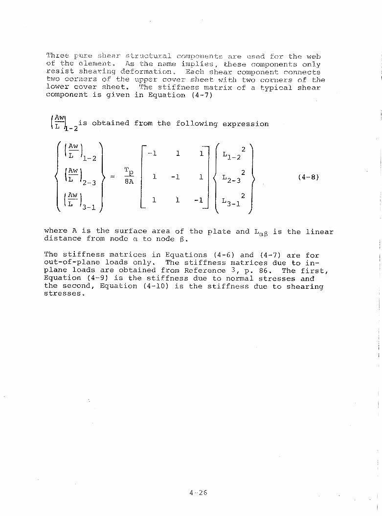
* sassaxqs hu?xeays oq anp ssauj3rqs ayq sr (OT-p) uo~qenbg ipuo~as ayq

pue sassaxqs Temxou 03 anp ssaujjrqs ayq ST (6-v) uopqenbz '7sx~z ay& "98 'd 'c aauaxaja8 mox3 paureqqo axe speo~ auqd

-ur oq anp sasrxqew ssaujjrqs ay& *Axuo speo~ aue~d-30-qno 203 arx? (L-v) pue (9-v) suoq.enb3 ur sasrxqem ssau33-y~ aya

*$ apou oq o apou moxj aDueqsrp xeaur-c ayq s? ~OT pup aqexd ayq jo eaxe asejzns ayq ST y aXayM

(6-$) uo-genb3 u~ uaapb s? quauodmoa zeays ~ea~dAq e 20 xrzqPm ssaussrqs ayL *qaays xaAoa xaMop

ayq. $0 sxauzoa OM? yg~~ gaays xsnoa zsddn ayq go sxauxe@ s~q sqaauuss qwawodwo~ nays yaez 'uoTqemxogap buyxeays qsTsaz Kxus s7uauadmoa asayq 'ss~~dm~ ameu ayq sy "quamala syq 2s q4~ ayq 202 pasn ~JP S~~U~UQ~UO~ TQxnqDnxqs reays axnd aaxyL

Yc '& -4 m 9) c e a m a -4 0 k m c a J

C N C u I a J k - 9 ) 7

- - 3 w u - a; & .Q 0

Yc 4J a a A

-4 S a0 & I O & W m a - P 0)

c 2 % 0 -4

al e, 0 5 -d 2

+' tr @ O W k al

w al $ w e vI aJ

O O O O O O O C

(I) cd

a &'

a d

t. .d i l -

The complete stiffness matrix i s cons t ruc t ed from the bending, t h e normal, t h e in-plane shear, and the ont-af-plane shear stiffness matrices, The s a t i o n is shown i n Equat ion ( 4 - % I ) ,

Equa t ion (4-11) produces a 15 x 15 s t i f f n e s s m a t r i x i n t h e member r e f e r e n c e f rame, where t h e o r i g i n i s a t node 1, t h e l i n e between nodes 1 and 2 forms t h e Xm a x i s and t h e p l a t e l ies i n t h e XmYm p l a n e .

4.2.3 P l a t e S t i f f n e s s P r o p e r t y S e n s i t i v i t y Mat r ix

F i v e p r o p e r t i e s of t h e p l a t e s t i f f n e s s may be c o n s i d e r e d as random v a r i a b l e s

G - modulus o f r i g i d i t y of t h e c o r e m a t e r i a l

Tc - t h i c k n e s s of t h e c o r e

T - t o t a l t h i c k n e s s o f t h e p l a t e P

E - modulus of e l a s t i c i t y of t h e f a c e s h e e t s

v - P o i s s o n ' s r a t i o

A s i n t h e c a s e o f t h e beam, noda l d imensions a r e n o t c o n s i d e r e d random.

The d e r i v a t i o n of t h e p l a t e e l ement s t i f f n e s s s e n s i t i v i t y m a t r i x f o l l o w s t h e same p r i n c i p l e a s t h a t used f o r t h e beam b u t t h e p rocedure i s s l i g h t l y d i f f e r e n t . A q u i c k g l a n c e a t Equa t ions (4-6, 7 , 9 and 10) w i l l r e v e a l t h a t most of t h e t i m e t h e p r o p e r t i e s l i s t e d above a r e found i n t h e c o n s t a n t s m u l t i p l y i n g t h e e n t i r e m a t r i x r a t h e r t h a n w i t h i n t h e m a t r i x e l ements themse lves . Only P o i s s o n ' s r a t i o l ies w i t h i n t h e s e c o n s t i t u e n t matrices.

L e t

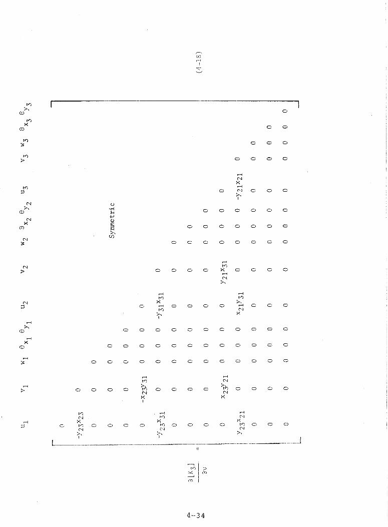
[K4] con ta ins only geometr ic terms and i s t h e mat r ix express ion i n Equation (4-10). [K1] i s a composite of t h e ma t r ix express ion f o r t h e t h r e e s h e a r webs and i s shown i n Equation (4-16). [K1] con ta ins only geometr ic terms t o o and thus w i l l n o t change i n form when [Kplafe] i s d i f f e r e n t i a t e d . The ma t r i ce s [ K ~ ] and [K3] both contasn t h e s i n g l e p h y s i c a l c o n s t a n t v and thus w i l l change form only when d i f f e r e n t i a t e d wi th r e s p e c t t o v. The

ma t r i ce s a [K21 and a [K31 a r e shown i n Equations (4-17) a v av

and (4-18).

ri " M rl rl xM

"2 0 0 0 +w (\I d X

dl" ,- ri?? I dl& I

C C C O O G C O

M O O G O 5 c c c c

M 4 rl

x" M X

C M O O O G x"

M G O 0 G M O 0 0 N c-4 N X X

!I

T h e s t i f f n e s s m a t r i x can now be w r i t t e n i n the fallswing form

The differentiation of (4-19) with respect to each of the five physical variables leads to the following five expressions

4,2,4 Rotatien of the P l a t e Pro..,erty S e n s i t F v i ty MztrFc~s 1 ----- - - -- -

The 3 w 3 matrixp [T I , describing the t r a r ~ s I o r m a t i o n from t h e Xm, Ym, Zm frame t o t h e X Y s , Zs frame i s developed i n t h e same manner a s t h a t used !?hr t h e beam w i t h t h e t h r e e node p o i n t s of t h e p l a t e corresponding t o t h e 3 r e f e rence points f o r t h e beam ( s e e F igure 4 - 2 ) . However, wi th t h e p l a t e element t h e r e i s no r o t a t i o n about t h e Zm a x i s even though t h e system pe rmi t s such a r o t a t i o n . Thus i n t ransforming from member t o system coord ina t e s t h e s t i f f n e s s ma t r ix e n l a r g e s from 1 5 x 15 t o 18 x 18. The r o t a t i o n ma t r ix , used t o t ransform Xm, Ym, Z m , Ox,, and O i n t o X s , Y s , Z s , OXs , O y s , and O Z s i s t h e r e f o r e

Ym

where t h e 3 x 3 [ y ] i s i d e n t i c a l t o t h a t developed f o r t h e beam.

The complete r o t a t i o n mat r ix f o r t h e p l a t e i s

[ R ~ ~ ~ ~ ~ ] i s a 15 x 18 mat r ix . The r e s u l t i n g s t i f f n e s s m a t r i x i n system coord ina t e s i s

A s in the case o f the beam, the r o t a t i o n procedure appl ied to the p l a t e stiffness matrlces carries over in the transformation of the partial derivatives into the system coordinates,

The equa t ion i s

- - lat

Once a l l of t h e e lements of have been completed,

they a r e s t o r e d i n a s i n g l e c a t r i x of t h e form shown i n Equation (2-16) and ( 4 - 3 ) . Since

a p i '"' 3 p l a t e i s symmetrical only t h e elements on t h e d iagona l and on one s i d e of t h e d i agona l a r e s t o r e d i n t h e format ion of

4 . 2 . 5 P l a t e Mass Proper ty S e n s i t i v i t y Matrix

A s i n t h e case of t h e beam, t h e mass of t h e p l a t e i s concent ra ted a t t h e nodes. The p l a t e element mass ma t r ix i s s e t up i n system coord ina t e s r a t h e r than t h e member r e f e r e n c e frame t o permi t t h e u t i l i z a t i o n of a d i agona l mass mat r ix . The unconstra ined mass mat r ix i s 18 x 18 t o accomodate s i x dynamic degrees of freedom a t each node.

The mass a t t h e node i s t r e a t e d a s t h e random v a r i a b l e and t h e p a r t i a l d e r i v a t i v e s of t h e mass elements a r e a l l taken wi th r e s p e c t t o t h e a c t u a l mass a t t h e node. The p rope r ty s e n s i t i v i t y mat r ix i s a column wi th up t o 18 elements a s shown. I t i s formed i n t h e same way a s t he beam except f o r t h r e e nodes r a t h e r than two. I t i s assumed t h a t t h e mass of t h e p l a t e i s e q u a l l y d iv ided between t h e t h r e e nodes.

(over )

a (m) - - ' a m ' p l a t e

4.2 .6 S y n t h e s i s of t h e S t i f f n e s s and Mass P r o p e r t y S e n s i t i v i t y M a t r i c e s -- P l a t e

S e c t i o n 4.1.5 d e s c r i b e s t h e s y n t h e s i s of t h e mass and s t i f f n e s s p r o p e r t y s e n s i t i v i t y m a t r i c e s f o r t h e beam. The p rocedure f o r t h e p l a t e i s i d e n t i c a l e x c e p t f o r t h e d imensioning. The e i g h - t e e n p o s s i b l e d e g r e e s of freedom of a p l a t e r e q u i r e s a n i n c r e a s e i n t h e number of rows r e q u i r e d t o hand le t h e p a r t i a l d e r i v a t i v e s f o r a l l t h e mass and s t i f f n e s s e l ements . Thus t h e t o t a l number of rows can i n c r e a s e t o 154 f o r t h e s t i f f n e s s e l ements and 18 f o r t h e mass e l e m e n t s .

For convenience i n t h e development of t h e VIDAP program it was d e c i d e d t o m a i n t a i n t h e p r o p e r t y c o v a r i a n c e m a t r i x a s a 9 x 9 m a t r i x . T h e r e f o r e i n t h e development of t h e p l a t e p r o p e r t y s e n s i t i v i t y m a t r i x where t h e r e a r e o n l y f i v e p r o p e r t i e s which can a f f e c t s t i f f n e s s and one which can a f f e c t mass, t h r e e columns w i l l c o n t a i n a l l z e r o s . The ar rangement of t h e columns i s shown below.

- - p l a t e

f up t o 1 7 1 rows

1 8 rows $.

The o r d e r of p h y s i c a l p r o p e r t i e s a c t i n g a s independen t v a r i a b l e s i n e a c h of t h e f i r s t f i v e columns moving from l e f t t o r i g h t i s G . T c r Tp: E , and v. The independent v a r i a b l e i n t h e n i n t h column 1s m ,

4 , 3 General S t i f f n e s s Matrix P

4 , 3 , $ General Discussion

A particular structure may, or may not, be composed of only beam and plate elements. For this reason we shall outline the procedure required to formulate the sensitivity matrix of a general structure.

In formulating the stiffness matrix of any structure we visualize a sequence of unit generalized displacements being applied successively at generalized coordinates creating corresponding generalized forces (stiffness coefficients). Therefore, the different component parts of the structure can be imagined to overlay in the stiffness matrix. In order to demonstrate this and clarify further discussion, consider the example structure shown in Fig. 4-6. The stiffness matrix for the structure (neglecting shear deformations) is

Symmetric

Therefore, any statistical uncertainty in member A would affect rows and columns l through 3 while any uncertainty in member B affects rows and columns 2 through 4 . If, for example, only the modulus of elasticity of member A was random the structure sensitivity matrix would be zero everywhere except rows and columns l through 3, i.e.

Figure 4-6 Example Structure

F i g u r e 4-9 Example S t r u c t u r e with

A d d i t i o n a l S t i f f n e s s Element

W e can conclude using this exampLe that only t h e rows and coleunns sf the stiffness matrix associated with the generalized displacements which define the shape characteristics sf the member whose parameter(s) are random are nonzero, By altering this physical system only slightly we can demonstrate the procedure used for a non-beam or plate random member.

Consider the structure shown in Figure 4-7. A vertical wire supplies additional stiffness to the beam at the midpoint. The structure (beam) stiffness matrix will now take the form

01

Inspection of this stiffness matrix reveals that uncertainty in the wire properties will only affect element (2 ,2 ) . Therefore, T o 0 0 0 7

This example demonstrates that if a general structural component which contributes stiffness to the structure has a random property, then only the row (s) and column (s) associated with generalized coordinates which prescribe its deformed shape are nonzero. And, a partial derivative of the elements in these rows and columns with respect to the random parameter result in the stiffness property sensitivity matrix.

; p = random wire property

0 0 ap

0 0 0 0

=L uoTqaaS u~ mayqoxd aydmes ayq uy pado~anap axe pue g uoyqaas ur pauye~dxa axe saoyxqem asaya

'saayxqem [sx] PUP [&J aqq 30 uorqexedaxd pueq dq paxnsse aq qsnm sxoqaanuabra PUP sanyenuahya ayq 30 sanrqenpap

~e?qx~d ayrl. yq~m 8 [[3l Ldz (TI ] [q qonpoxd ayq uy squamaTa ayq 30 dqyy~q?qedmoa ayq 'ppasn sr xyxqem ssauggrqs Axexqyqxe ue 21

=L uorqaas UT ma~qoxd a~dmes ayq ur u~oys ST qanpoxd syyq 30 quawrdo~anap ayq 30

a~dmexa uy *xTrqem aq.ljurs e se paxaqua sy (PZ-2) pu~ (02-2) suo?q~nbz uy , [a] [dz ] 133 qanpoxd aqq ley? sueam axnpaooxd

syy~ *mexhoxd ayq oquy xrxqewr aybuys e se paxaqua aq pue Q~aqaboq pa~ydrq~nm aq Bwexljozd ayq aprsqno padoaanap aq qsnm xrxqem aoueTxenoo Wqxadoxd ayq pue xyxqem Aqynyqysuas dq~adoxd aw 'ssaumopuex pa~3raads amos qqrM xTxqem ssauggyqs Xxexq~qxe

ue asn 03 sy uoyqdo ayq 31 's3uamaq.a ~exauafi 203 sasrxqem ssausgg-s Xxexq~qze pue squamaTa aqe~d pup meaq go sarqsrzaqae -3w3 ~e3~7sy3e3s ay3 sxpuey 03 paufi~sap ST ~e~xbozd ~V~IA aqL

5,8 PROPERTY COVARIANCE MATRICES

5 , 1 In t roduc t ion

I n Sec t ion 4 methods were presen ted which developed t h e p a r t i a l d e r i v a t i v e s r e l a t i n g m a s s and s t i f f n e s s ma t r ix elements t o s p e c i f i c beam o r p l a t e p r o p e r t i e s . This completed t h e p a r t i a l d e r i v a t i v e development necessary f o r r e l a t i n g p h y s i c a l pro- p e r t i e s t o modal p r o p e r t i e s by means of Equations (2-17) and (2-18) i n Sec t ion 2. The remaining s t e p t h e r e f o r e i s t h e c o n s t r u c t i o n of t h e covar iance mat r ix f o r t h e p h y s i c a l p r o p e r t i e s t o be incorpora ted i n t o Equations ( 2 - 2 1 ) and ( 2 - 2 2 ) . The g e n e r a l form f o r t h e p rope r ty covar iance mat r ix i s shown below.

I f p r o p e r t i e s such a s E , v , I , t , A , e t c . a r e s t a t i s t i c a l l y independent, t h e c o r r e l a t i o n c o e f f i c i e n t s , p i , , van ish and t h e ma t r ix i s d iagona l . However, i n most ca ses c o r r e l a t i o n does e x i s t because, f o r example, A , 12, 13: and J depend upon t . This covar iance v a r i e s wi th t h e cross-sectional conf igu ra t ion of t h e element and s i n c e t h e v a r i e t y of con f igu ra t ions i s l imit less t h i s p a r t of t h e s t a t i s t i c a l o p e r a t i o n i s computed o u t s i d e t h e VIDAP program and provided a s an i n p u t i n mat r ix form. The remainder of t h i s s e c t i o n i s devoted t o t u t o r i n g t h e u s e r i n t h e development of t h e s e covar iance ma t r i ce s .

5 - 2 Development s f a Prope r ty Covariance Matrix for a Tubular - ------ B e a m Element

The p h y s i c a l p r o p e r t i e s used t o d e s c r i b e the s t i f f n e s s m a t r i x f o r a beam a r e E , A , 1 2 , 13, v, SF2, SF3, and J. I n t h e ca se of a tube t h e p r o p e r t i e s A, 1 2 , 13 , and J a r e a l l dependent upon t h e t h i ckness , t , and t h e i n s i d e r a d i u s , r , of t h e tube .

For t << r

m = p2nrt Lo 1/2 (beam mass i s s p l i t between t h e two nodes, t h i s m i s f o r a s i n g l e node)

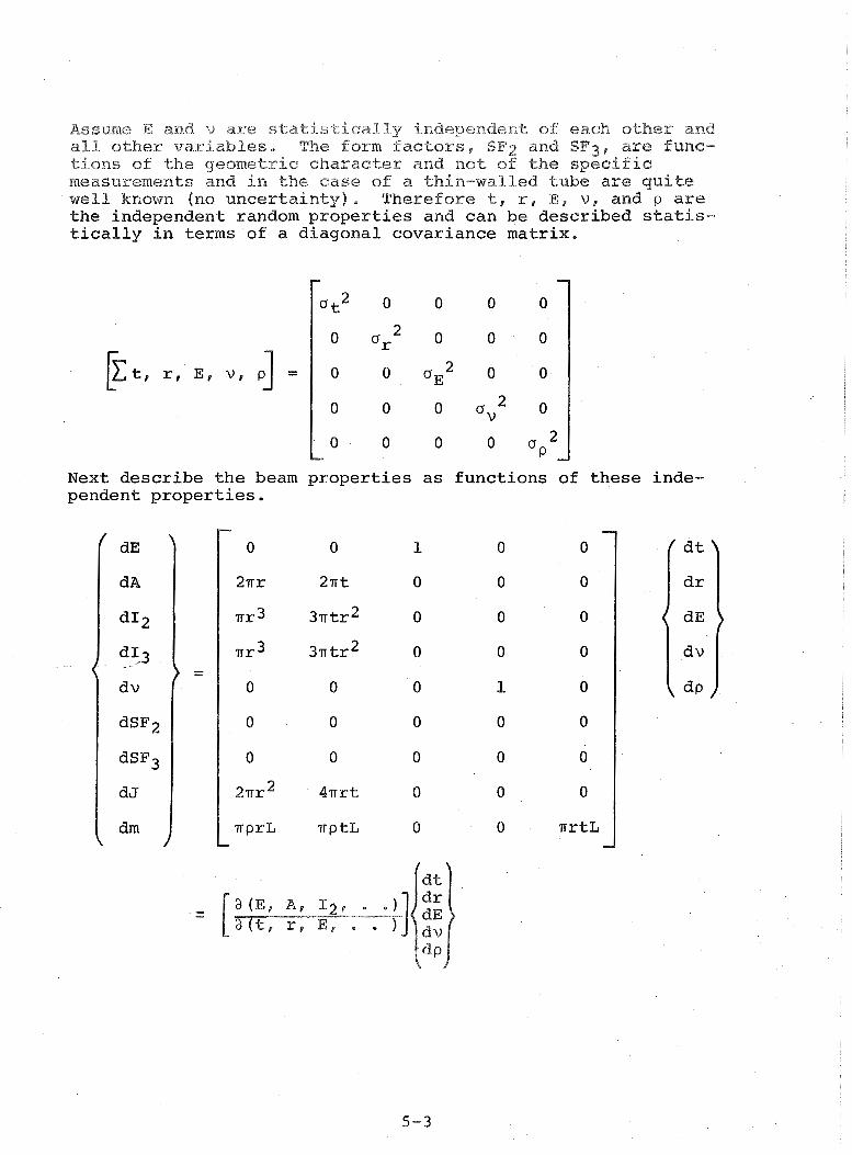
A s s m e E and v are statistically independent o f each other and all other variables, The form factors , SF2 and SF3, are functions of the geometric character and not sf the specific measurements and in the ease sf a thin-walled tube are quite well known (no uncertainty), Therefore t, r, E , v, and p are the independent random properties and can be described statistically in terms of a diagonal covariance matrix.

Next describe the beam properties as functions of pendent properties.

these inde-

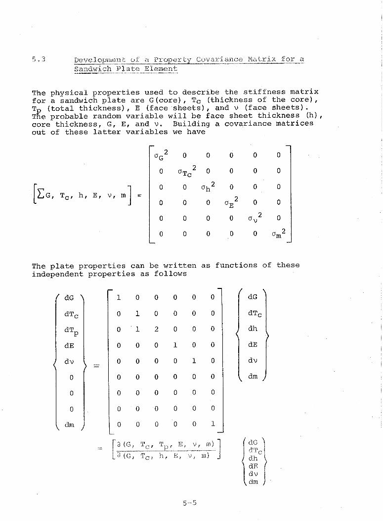
5 , s Sandwich Plate Element

The physical properties used to describe the stiffness matrix for a sandwich plate are G(core), Tc (thickness of the core), T (total thickness) , E (face sheets) , and v (face sheets) . TRe probable random variable will be face sheet thickness (h), core thickness, G, E, and v. Building a covariance matrices out of these latter variables we have

The plate properties can be written as functions of these independent properties as follows

Recall that the proper ty covariance matrix is always 9 x 9 and therefore the properties affecting the plate stiffness are in the first five rows in the above matrix, whereas the mass is in the ninth rew. The resulting covariance matrix w i l l have a13 zeros i n the 6 t h , 7 t h , and 8th rows and columns b u t t h i s w i l l be conformable w i th

a s developed i n Sec t ion 4 . 2 . 6 . p l a t e

Thus

uGt 'pr ej[xGr Tc, h , --I[ a ( ~ r ~ , r T p r e [''I = [ a ( G f Tcf h r * - 1 a ( G , Tc, h r * 0 ) "I' A s mentioned i n Sec t ion 4 , t h e mass of t h e p l a t e i s d iv ided equa l ly between t h e t h r e e nodes. The va r i ance of t h e mass included i n t h e covar iance mat r ix above i s f o r one node on ly and hence i n p repar ing t h e d a t a use one- th i rd t h e s tandard d e v i a t i o n of t h e mass of t h e t o t a l p l a t e .

6 , l Cons t ruc t ion of t h e Mass and S t i f f n e s s Matr ices

I n Sec t ion 2 . 2 . 1 a t r u s s example was used t o d e s c r i b e t h e development of t h e s t i f f n e s s mat r ix . I t was noted t h a t t h e f i r s t s t e p i n t h e s t i f f n e s s mat r ix development was t h e con- s t r u c t i o n of t h e unde le ted s t i f f n e s s ma t r ix shown i n Equation (2 -8 ) and repea ted i n Equation (6-1) below,

- - - - ,---- L - - - - . - . - -

[K] undele ted = 1 [2-11 I bm21 I [2-31 ,

where t h e submatr ices [i- j] a r e t h e nodal s t i f f n e s s m a t r i c e s . * The undeleted mass mat r ix i s a d iagona l ma t r ix a s shown

The dimension of t h e undele ted mass o r s t i f f n e s s ma t r ix i s 6 x no. of nodes. The dimension of t h e dynamic mass o r s t i f f - ness ma t r ix i s t h e dimension of t h e undele ted mat r ix l e s s t h e number of r e s t r a i n t s upon t h e system. To reduce t h e unde le ted ma t r ix , t he rows and columns corresponding t o each cons t r a ined degree of freedom a r e removed and t h e remaining columns and rows a r e s h i f t e d t o f i l l i n t h e vo ids t o form t h e sma l l e r ma t r ix , This method only permi t s c o n s t r a i n t s t h a t a r e a l i g n e d wi th t h e coo rd ina t e s , Fu r the r s o p h i s t i c a t i o n of t h e c o n s t r a i n t s i s p o s s i b l e b u t w a s n o t considered necessary i n t h i s a n a l y s i s .

[MI undeleted =

The mass and stiffness matrices of large dynamic models r e q u i r e a la rge amount of csmputer storage and as a r e s u l t methods have been dev ised t o manipulate t h e form and reduce the storage requirement , VIDAP h a s been designed to handle 300 degree-of freedom systems, The d iagona l mass ma t r ix i s s t o r e d a s a colurnn

I I I

6 1-1 J I C03 I 101 I . - - - - I - - - - - , - - - - - ' - - - [oI I r 2-2 3 1 r01 I .

"Node numbers must be consecut ive and s t a r t wi th 9.

6 - 1

and the symetr ie and banded stiffness matrix i s stored vert- i c a l l y as a semi-band i n a r e c t a n g u l a r format, These formats are shown p i c t o r i a l l y in Figure 6-1,

System Mass Matrix VIDAP Form

System Stiffness Matrix VIDAP Form

Figure 6-1 Storage of the System Mass and Stiffness Matrices in VIDAP

6,2 Compatibility

The purpose of VIDAP, as discussed earlier, is to produce statistical characteristics of eigenvalues and eigenvectors of large systems based upon the statistical characteristics of properties of individual structural components. This is accomplished by the development of partial derivatives used in a matrix chain as shown below

syst I where the presuperscript [(i) ] represents perturbations in the system due to perturbations in the properties of structural member, i.

The two large matrices in Equation (6-3)

submatrices as shown. The two matrices

were developed in Section 4 and synthesized into

[a (F;py) ] in Subsections 4.1.5 and 4.2.6. The mass and stiffness

elements are all oriented into system coordinates although the matrix element numbering is oriented to the local coordinate sys tern.

The components of the matrices and ["'"'"' ] a (m) sys t ,

are derived according to the methods developed in Section 3. These matrix components are developed, however, according to addresses in the system mass and stiffness matrices and it is here where a procedure must be developed to make compatible the partial derivatives in the two successive matrices of Equation (6-3).

Before continuing with the compatibility development, consider first the input and dimensional requirements, The vector fdX - \ represents derivatives sf all the eigenvahues and eigen-

a dx B vector components sf i n t e r e s t to t h e program u s e r , The use r of VSDAP c a n select up to 100 eigenvalues and/or eigenvector

components in several combinations to be evaluated statistisal%y, The only restriction is that the selected components of any eigenvector must be in either one or two groups. For example if statistical characteristics of components of the jth eigenvector are desired, they must be obtained using one of the following options.

Eigenvector Option 1

statistical characteristics of all (x.1

3

Option 2

statistical characteristics of one section of {x-1, i.e. consesutive elements

x(i+~) jr . . . (i+2) j r

Option 3

statistical characteristics of two sections of {xj} i.e. consecutive ele-

ments Xij' (i+I) j (i+2) j r . . .

and

Xkjr X(k+l)jr

x(k+2)jr " * "

The number of rows and the notation of the rows in the matrix

correspond to the eigenvalue and eigenvector statistical data requested by the user. Hence the matrix will not exceed 100 rows (although the number of degrees of freedom of the system can far exceed this). The output of VIDAP will group together the data from the same eigenvalue and eigenvector. That is

the successive rows of (i) will have Xi, xli, x2i, . . Aj, XI,, x2jf etc.

Each column of has a single independent variable st

in all the partial derivatives whereas each row has a single dependent variable, This is shown below,

where the subscripts ( )rs are in system coordinates.

The dependent variables in (i) a (kr .m) I must correspond to the independent variables in (l)a x) 1 the problem is rip: 1*:m1 sysf that the coordinates of the structural element may be found in a number of different locations in the structural coordinates. For example consider a beam element with end points at node 3 and node 5 of a six-node system. Let each node have three restraints. The symmetrical element and system matrices will be as shown in Figure 6-2.

The stiffnesses of the particular beam are not the only stiffnesses located in the addresses shown in Figure 6-2. However, if this beam joining nodes 3 and 5 is allowed to vary while all of the rest of the system remains constant, then the derivatives associated with these addresses will be exclusively those of this particular beam element.

If the address of a stiffness element is known in the system stiffness matrix, the appropriate partial derivatives can be developed according to the methods of Section 3, To do this an accounting procedure must be used to find the locations of the beam stiffness elements in t h e system stiffness matrix.

The procedure is as follows:

(1) The t w o nodes of the beam are treated i n ascending order, i ,e, 3 comes before 5,

System Stiffness Matrix

Structural Member Stiffness Matrix (6 constraints)

- - "1 beam

Node 3

"r Node 5

Figure 6-2 B e a m Element Stiffness Locations

( 2 ) The n m b e r of uncons t ra ined coordinates are counted i n ,319 the nodes p r i o r to the l o w e s t node of t h e b e m , En t h i s case there are 6 unconstra ined cosr- d i a a t e s before node 3 , The sum s f t h e s e coo rd ina t e s g ives t h e number used t o determine t h e f i r s t row i n t h e system s t i f f n e s s mat r ix .

( 3 ) The number of unconstra ined coord ina tes i n t h e f i r s t beam node a r e counted and t h i s number i s used t o e s t a b l i s h t h e number of consecut ive rows i n t h e s t i f f n e s s mat r ix which a r e occupied by t h e s t i f f n e s s of t h i s f i r s t node.

( 4 ) The number of unconstra ined coo rd ina t e s between t h e two beam nodes a r e counted t o e s t a b l i s h t h e row number i n t h e system ma t r ix corresponding t o t h e s t i f f n e s s e s of t h e second node of t h e beam.

(5 ) The number of unconstra ined coo rd ina t e s i n t h e second beam node a r e counted and t h i s number e s t a b l i s h e s t h e consecut ive rows i n t h e s t i f f n e s s mat r ix occupied by t h e s t i f f n e s s e s of t h e second beam node.

To implement t h i s procedure two new ma t r i ce s a r e in t roduced t o t h e a n a l y s i s . These a r e c a l l e d [KR] and [KS] and a r e s t r i c t l y i n t e r n a l t o t h e program.

[KR] and [KS] a r e square ma t r i ce s having t h e same number of rows and columns a s t h e r e a r e unconstra ined coord ina tes i n t h e member ( i n t h i s c a s e , t h e beam) . Each row of [KRJ has only a s i n g l e number corresponding t o a row i n t h e system s t i f f n e s s mat r ix . Each column of [KSJ has on ly a s i n g l e number and t h e s e correspond t o s i n g l e columns i n t h e system s t i f f n e s s mat r ix . The development and implementation of t h e s e two ma t r i ce s i s a s fo l lows:

( a ) From s t e p s ( 3 ) and ( 5 ) above, count t h e number of unconstra ined coo rd ina t e s i n t h e beam and s i z e [KR] accord ing ly

I number of

[KR] = unconstra ined coo rd ina t e s

91 P

number of unconstrained

-coordinates +-

(b) From step (2) find the number of the row containing the first member stiffness in the sys t em matrix and e n t e r this mmber in the first asow of Fg,

r r r r r r

[ K R ] =

(c) From step (3) take the number of unconstrained coordinates in the node and number the same number of rows in [KRJ consecutively.

r r r r r

r+l r+l r+l r+l r+l

[ K R ] = r+2 r+2 r+2 r+2 r+2 1 (d) From steps (2), ( 3 ) , and (4) count the total number

of rows in the system stiffness matrix preceeding the stiffness of the second node of the member. Let s be the row number corresponding to the first row in the stiffness matrix of this second node.

r r r

r+l r+l r+l *

[ K R ] = r+2 r+2 r+2 * = 1 S S S

(e) Complete [ K R ] by numbering the remaining rows consecutively, s+l, s4-2, etc.

r r r

r+l r+l r+l

r+2 r-t-2 r i -2 *

S S S

s+% s-4-P s f 1 - s+2 sa-2 s+2 *

~ook now at [K,] beam in F i g u r e 6 - 3 , I f we move across t h e f i r s t row, then s t a r t again at the diagonal and corfiplete t h e second row and s o on w e can form a c s l m n s f s t i f f n e s s elements wi thout d u p l i c a t i o n because of symmetry,

-l

The p a r t i a l d e r i v a t i v e s i n t h e mat r ix J , Equation (4 -3 ) ,

a r e o rdered v e r t i c a l l y i n t h i s way. Thus i f w e form a column of i n d i c e s from [KR] and [KS] by going a c r o s s t h e rows of [KR] and [KS] i n t h e same way, we w i l l have a set of i n d i c e s f o r t h e system coord ina t e s which a r e i n a column compatible wi th t h e p a r t i a l d e r i v a t i v e s of t h e member s t i f f n e s s e s . The column of i n d i c e s is shown below.

Samples d i scussed on t h e previous pages

The v e c t o r , { i n d . ) , p rov ides t h e i n d i c e s a s s o c i a t e d wi th krs and m,, i n computing t h e p a r t i a l d e r i v a t i v e s f o r e igenva lues and e igenvec to r s i n Equations (3-8) , (3-9) , (3-29) , and (3-30) . This e n t i r e procedure i s p i c t u r e d i n t h e Slow diagram i n F igure 6-4 .

Because only t h e d i agona l and one t r i a n g u l a r h a l f of t h e ma t r ix a -[K] ( see Equations (4-2,3) ) a r e used i n developing a p j some compensation must be made f o r t h e omi t ted d e r i v a t h e f i n a l mat r ix m u l t i p l i c a t i o n t akes p l a c e , This i s accomplished by p u t t i n g i n t ~ the spaces occupied by t h e p a r t i a l d e r i v a t i v e s having r = s , the s m a f ) - + a x i a x i

a ( Irs + - a x ; a k r ~ akssr;

of t

he

mem

ber

st

iffn

ess

mat

rix

Co

nst

rain

t ta

ble

fo

r e

ac

h n

od

e in

th

e s

tru

ctu

ral

mo

del

. *

Use

r re

qu

est

s th

e

sta

tist

ics

of

"The

p

rog

ram

ass

um

es

6 de

crre

es o

f fr

eed

om

a

t e

ac

h n

od

e b

efo

re

co

nst

rain

ts a

re a

pp

lie

d

eig

en

va

lue

s an

d

eig

en

ve

cto

rs

Fig

ure

6-4

C

om

pat

ibil

ity

Pro

ced

ure

fo

r th

e D

evel

op

men

t of

Eig

en

va

lue

ne

cto

r P

arti

al D

eriv

ativ

es

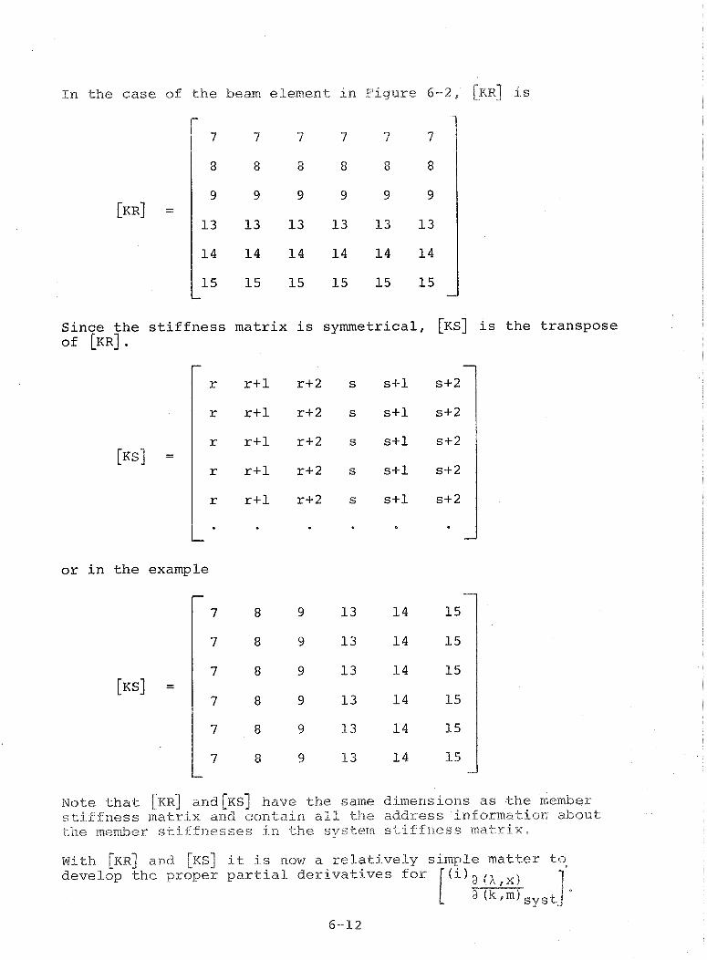
I n the case of the beam element in Figure 6-2, [ b l C ~ ] is

Since the stiffness matrix is symmetrical, [KS] is the transpose of [KR] .

or in the example

Note that [KR] and[^^] have the same dimensions as the member stiffness matrix and contain a l l the address information about the member stiffnesses in the system stiffness m a t r i x ,

With [KR] and [KS] it is now a relatively simple mat te r to develop the proper partial derivatives for

Thus the subscripts in the vgctor {in$,) are used i n both

orders. A typical r o w in ' (i' a " would t h e n apQear as shown be low, [ a (krrs, 1

a x i The expression is symmetrical and thus akrs

ax i a x i a x i axji + - = 2 - is not symmetrical

akrs aksr akrs akrs

however, but the sum has been derived as shown in Equation ( 3 - 3 0 ) .

6 - 3 tar P a r d i a l Derivatives ---- - .

The previous section described how compatibility relations were used for selecting the proper indices for eigenvalue/veetor partial derivatives. It was pointed out how these indices were used with certain equations in Section 3 to compute and order the partial derivatives. The purpose of this section is to describe breifly the operations involved in the development of partial derivatives for the eigenvectors. Whereas the expressions for the eigenvalue partial derivatives, Equations (3-8) and (3-9), are quite straightforward, those for the eigenvectors are more complex and involve considerable computation. In fact, the eigenvector partial derivative computation involves the largest single operation in the VIDAP program.

The eigenvector partial derivatives are developed in two steps:

(1) One element of the eigenvector is held fixed while partial derivatives are developed for the other elements relative to the fixed element. The equations for partials with respect to diagonal and off-diagonal elements in the stiffness matrix are (from Section 3):

(2) The partial derivatives developed in Step (1) are modified to maintain constant generalized mass and in so doing the fixed element is permitted to take on a non-zero value. The expression is:

* I s U } represents omission of the uth element, [-U] represents omission of the u t h row and column, In VPDAP u = 0, but. can be extended to operate for any value, **I "1 represents represents replacement of the u t h e l e m e n t by a zero, Hence a vector { "1 has n elements whereas !-U1 has n-L elements.

In the i n t e res t o f minimizing the computer s torage, the matrix '--u2 w h i c h i s s p m e t r i c a l , i s formed f r o m [K] , EM],

L'i and hi and s t o r e d i n a semi-band, The ope ra t ion i s shown i n

Figure 6-5. , which i n i t s symmetrical form i s ( n - l ) x (n-1) , i s a l s o of o r d e r n-1 and t h u s capable of i nve r s ion .

The number of o p e r a t i o n s i n t h e s o l u t i o n of Equation (6-5) o r

(6-6) can be minimized by r e t u r n i n g [ G ~ ] t o t h e le f t -hand s i d e of t h e equa t ion and by s o l v i n g t h e column of equa t ions s imul taneous ly - - r a t h e r than by i n v e r t i n g A decomposit ion procedure involv ing banded ma t r i ce s was s e l e c t e d f o r t h e s o l u t i o n of (6-5) and (6-6) . The decomposit ion method (Ref. 7 ) breaks rFiul i n t o t h e produc t of t h r e e ma t r i ce s . L -1

where S] i s an upper t r i a n g u l a r mat r ix wi th u n i t d iagona l and [D f i s a d i agona l b u t no t u n i t a r y ma t r ix .

The decomposition procedure a s o u t l i n e d i n Reference 7 pe rmi t s t h e ma t r ix [FYU! t o have nega t ive numbers on t h e d iagona l . Qther decomposit ion m e t ods (Ref. 4 ) which use only t h e produce Ls] ' IS] (with t h e d i agona l non-unitary) , i n c o r p o r a t e a square- r o o t o p e r a t i o n i n t h e s o l u t i o n which w i l l n o t work wi th t h e nega t ive d i agona l e lements .

The second s t e p of t h e p a r t i a l d e r i v a t i v e development involves no s p e c i a l o p e r a t i o n s and t h e r e f o r e does no t r e q u i r e f u r t h e r e l a b o r a t i o n .

[K], and Xi

Form [Fi]

-u Form [Fi ]

Figure 6-5 Formation of Banded [F;~]

6-16

6 - 4 Program Operation

The operation of V I D A P i s summarized i n t h e f lowchar t in P i g , 6-6. The fol lowing exp lana t ion summarizes t h e ope ra t ions i n each s t e p and r e f e r s t h e r e a d e r t o o t h e r s e c t i o n s of t h e r e p o r t f o r e l a b o r a t i o n where necessary.

A s i n p u t t o t h e program, t h e u s e r provides t h e s t r u c t u r a l s t i f f n e s s ma t r ix , t h e mass m a t r i x , e igenva lues and e igen- v e c t o r s of t h e modes of i n t e r e s t , t h e number of nodes i n t h e s t r u c t u r e , t h e p h y s i c a l l o c a t i o n s of t h e nodes, and a l i s t of coo rd ina t e c o n s t r a i n t s f o r each node.

S tep 2

The u s e r r e q u e s t s s t a t i s t i c s of t h e f requenc ies and modes of i n t e r e s t . The t o t a l number of e igenvalue and e igen- v e c t o r components can range upwards t o 1 0 0 .

S tep 3

B e a m and p l a t e p roper ty d a t a a r e e n t e r e d f o r t h e development of t h e p a r t i a l d e r i v a t i v e s . Proper ty covar iance m a t r i c e s a r e i n p u t a s 9 x 9 m a t r i c e s . The node numbers must be provided f o r each random member.

S t ep 4

I f an a r b i t r a r y s t i f f n e s s ma t r ix i s used, a covar iance ma t r ix f o r s t i f f n e s s and mass p r o p e r t i e s must be developed o u t s i d e t h e proqram. The e x t e r n a l development of t h i s - - -

[ ] removes t h e need f o r t h e p rope r ty covar iance kr,m

m a t r i x and t h e development of 8 k r , m ] . [KR] and

[KS] must be computed case and provided a s i n p u t d a t a .

S tep 5

Program o p e r a t i o n begins when t h e ques t ion i s asked about t h e type of e lement . I f i t i s a beam o r p l a t e , t h e program

a t a i n S tep 3 and proceeds t o compute

i n Step 6 , I f it i s an a r b i t r a r y s t i f f n e s s

matrix, the program bypasses S t e p s 6 and 7 and uses the d a t a provided i n S t ep 4 ,

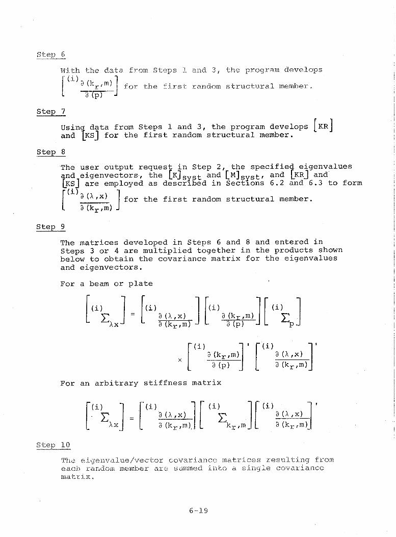
Step 6

With the data from Steps E and 3, the program develops -

fo r the first random structural member.

Usin data from Steps 1 and 3, the program develops [KR] and TKSJ for the first random structural member.

Step 8

The user output request in Step 2, the specified eigenvalues and eigenvectors, the [KJ,~,~ and L M ] ~ ~ ~ ~ ~ and LKRJ and LKSJ are employed as descrrbed in Sectlons 6.2 and 6.3 to form [ a for the first random structural member.

a (kr ,m) 1 Step 9

The matrices developed in Steps 6 and 8 and entered in Steps 3 or 4 are multiplied together in the products shown below to obtain the covariance matrix for the eigenvalues and eigenvectors.

For a beam or plate

For an arbitrary stiffness matrix

Step 10

The eigenvalue/vector covariance matrices resulting from each random member are s ed into a single covariance matrix,

T h e covariance matrix computed i n Step 9 i s stored, and t h e p r ~ e e d u r e s t a r t i n g i n Step 5 is repeated for each random structural member.

The covariance matrix resulting from Step 11 is used to compute the standard deviations and the correlation matrix of all the requested output data. Equation (2-10) is used to transform standard deviations of eigenvalues into standard deviations of frequencies. The final output contains mean values and standard deviations of eigenvalues, frequencies, and eigenvector components.

EXAMPLES AND VERIFICATION

7.1 Me thodology

Verification of the linear statistical model can be made in two ways which are quite independent of each other. The first method involves developing partial derivatives numerically by perturbing a sample problem and comparing these partial derivatives with those computed within the program. The second method is to use the Monte Carlo method to generate the statistics of a sample system and to compare the results with the statistical characteristics generated by VIDAP.

The above methods were used in evaluating two sample problems: a simple longitudinal rod and an SII longitudinal vibration analysis provided by the George C. Marshall Space Flight Center."

The selection of the four degree-of-freedom longitudinal rod was convenient because this problem had been thoroughly checked earlier in the development of the J. H. Wiggins Company PASS I (Probabilis- tic Analysis of Structural Systems) Program. Thus, the partial derivatives developed by a proven program could be compared with those developed by VIDAP. The SII longitudinal vibration problem gave the opportunity to demonstrate VIDAP on a larger system and in an area of interest to NASA.

7.2 Four Degree-of-Freedom Longitudinal Vibrations

The longitudinal rod studied in this example is shown below in Fig. 7-1.

Figure 7-1 Four Degree-of-Freedom Longitudinal Fixed-Fixed Rod

The mass arid stiffness matrices are as follows. (Note that the mass matrix is non-diagonal and is based upon the consistent mass matrix approach described in Reference 8.)

-- - either of a z F ~ b ~ e m s contain the plate or beam elements discussed in Section 4 since the checkout of this section of VIDAP was n o t successfully completed at the writing of this report .

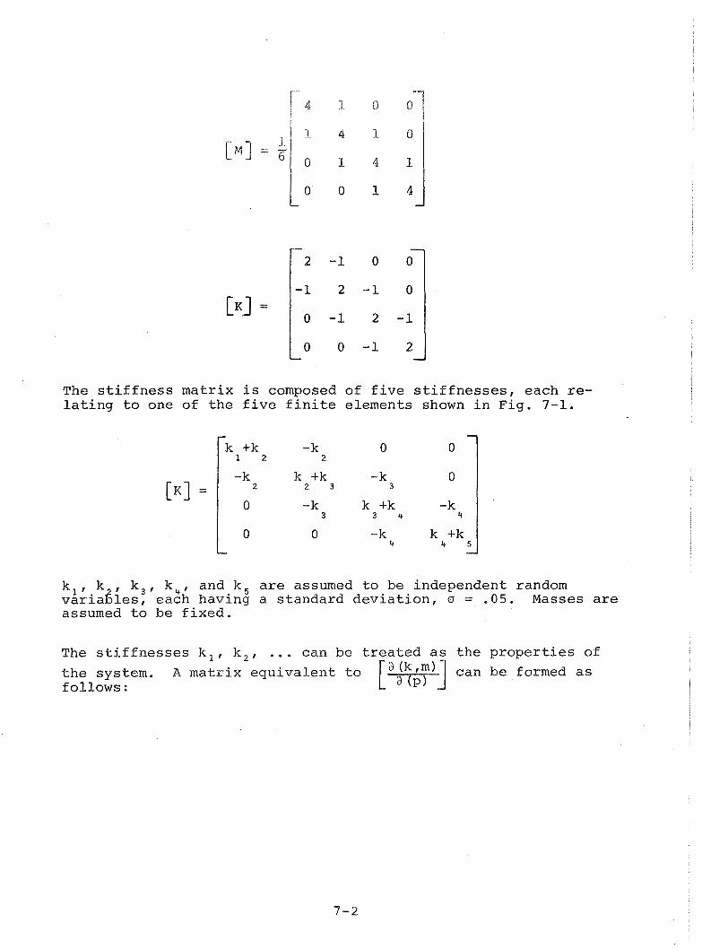
The stiffness matrix is composed of five stiffnesses, each re- lating to one of the five finite elements shown in Fig. 7-1.

k,, k , k 3 , k and k, are assumed to be independent random varia%les, each having a standard deviation, a = .05. Masses are assumed to be fixed.

The stiffnesses k , , k,, ... can be treated as the properties of the system. A matrix equivalent to C can be formed as follows:

h a s n i n e columns which make it compat ib le w i t h a (kg)

VIDAP.* Note t h a t a l l t h e s t i f f n e s s e l ements on and above t h e d i a g o n a l a r e c o n s i d e r e d . However, o n l y t h e d i a g o n a l mass e lements a r e c o n s i d e r e d because i n t h e d e s i g n of t h e program it was a n t i c i - p a t e d t h a t most mass matrices would be d i a g o n a l , and t h e p a r t i a l d e r i v a t i v e m a t r i c e s cou ld have s m a l l d imensions i f mass p a r t i a l d e r i v a t i v e s were r e s t r i c t e d t o t h e d i a g o n a l ,

*VPDAP p e r m i t s t h e inpblt of n i n e random p r o p e r t i e s . The A ( 1 , J )

matrix (equivalent to ) i n s t e p 1 8 of Appendix B

mus t a lways have n i n e columns even though, as i n t h i s c a s e , a l l n i n e a r e n o t n e c e s s a r y ,

The covariance matrix far t h i s system o f f i v e independent random variables has t h e va r i ances of the f i v e success ive kits down t h e d iagonal , The remaining four zeros on the diagonal account for t h e remaining f o u r random v a r i a b l e s which a r e a v a i l a b l e i n VPDRP b u t n o t used in t h i s problem.

I 9 columns *I The [KR] ma t r ix i s ( s e e Sec t ion 6 .2)

[KS] i s t h e t r anspose of [KR] . The r e s u l t s of t h e VIDAP run a r e shown i n Tables 7-1 and 7-2. The s t a t i s t i c s of t h e e igenva lues compare e x a c t l y wi th t hose of PASS I , and t h e r a t i o of t h e s t anda rd d e v i a t i o n of t h e frequency t o t h e frequency i s a c o n s t a n t a s would be expected by a cha in of uncorre- l a t e d s t i f f n e s s e s (Reference 9 ) . The s t a t i s t i c s of t h e e igen- v e c t o r s do n o t ag ree wi th t h e PASS I ou tpu t because PASS I f i x e s t h e f i r s t element i n each e igenvec to r , thus making t h e s t a n d a r d d e v i a t i o n of t h i s element zero and changing t h e o t h e r e lements i n a manner d i s c u s s e d i n Sec t ion 3.

The e igenvec to r p a r t i a l d e r i v a t i v e development i n VIDAP i s i n two steps, t h e first of which holds the first element of the eigen- v e c t o r constant in a manner analogous to PASS I,

The e q u a t i o n s leading to the partial derivatives in PASS I are d i f f e r e n t (see Reference I ) , but t h e r e s u l t s should be t h e same, The f i r s t - s t a g e p a r t i a l d e r i v a t i v e s developed by VIBAP were corn- pared wi th t hose developed by PASS I , and t h e two programs d i d

*qua3 ;cad 02 oq 01 30 "3 UT sabueys 303 aTqeuosea2 s? Aq7.xeauy-r 30 uorqdurns -se ayq 8qsea-r q~ uraqsAs s~yq lo3 'qeyq 3uapy.a ST 21 *ITy quaura-ra

ssaugj~qs ayq u? sabueya quaa lad 'sn sauamaxa xoqaanuab~a a-c3?3 -ads ur sabuey~ quas lad ~oys 5 pue p'cF"~-~ saxnbyd *saArqenT.xap

~~rqxed ay2 go A~TIP~UTT $0 35~~1 ayq. auTuexaqap oq xTzqem ssau3zTqs ayq ur squamaaa so appw axaM suor~eqxnqxad quapusdapu~ go qas y

"qndans dva~~ aqq qq~~ paaz5-e sxafisue ayq pu@ Appaqndwsa pupy uayq SQA quamdo~anap anTqPnyxap ~e~qx~d ayq 30 a6eqs puaaas ayL -saznby~ que3~g~uG~s xnoz oq. aax5~ paapuT

ojo in P- alm cz m

crpn a13) 4- u3

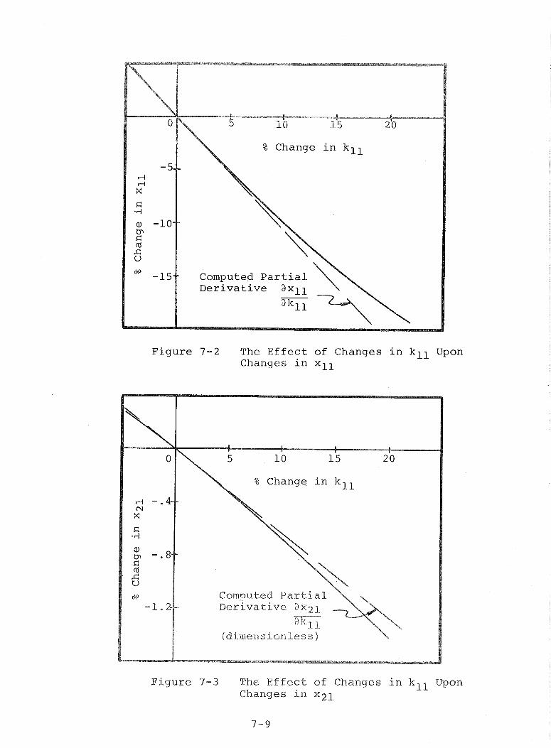
Figure 7-2 The Effect of Changes in kll Upon Changes in xl l

% Change in kll

Computed Parti Derivative axZl

(dimensionless)

Figure 7 - 3 The Effect of Changes in k E k Upon Changes in x 2 1

9-9

Figure 7-4 The Effect of Changes in k l l Upon Changes in x31

Figure 7-5 The Effect of Changes in kll Upon Changes in x p l

7-10

7 - 3 ---- S $1 Longitudinal -- Vibration -

7 , 3 , % The Problem and VEBAP Solution

The mass and stiffness matrix data for the 26 degree-of-freedom S I1 Longitudinal Vibration Analysis are presented in Table 7-3. In this particular problem a section of the stiffness matrix is considered uncertain. This section is located in the upper left- hand corner and the relationships between the stiffnesses are shown more specifically by the matrix below. kl and k2 are considered to be random variables.

The VIDAP program can take any combination of rows and columns in the stiffness and provide eigenvalue/vector statistics based on the property statistics. In this problem the first three rows and columns forming the 3 x 3 section is to be treated by VIDAP. Looking at the stiffness matrix, the following matrix,

L- , can be developed.

TABLE

7-3

5 II L

ON

GIT

UD

INA

L

VIB

RA

TIO

N

AN

AL

YS

IS

RE

VIS

ION

T

= 3

40

SEC

MA

SS

M

AT

RIX

CO

LU

MN

( 1

1

CO

LJ

MN

~ 2

)

CO

LU

YN

I 3)

CO

LU

MN

( 4)

CO

LU

MN

( 5

1

CO

LU

MN

( 6

) C

OL

UM

N(

7)

CO

LU

MN

[ 8) C

OL

UM

N1

9

)

CO

LUM

""IN

(10)

1

a0

64

0+

61

@

,80

00

0

.GO

00

0 e

OO

G0

0.0

00

0

0.O

OO

G

0.0

00

0

0.0

00

0

0.0

00

0

01 0

0630

O

a0

00

0

BoOQ98+02

0.0

00

0

Oe

OO

OO

0

.00

00

0

.00

00

0

.00

00

0

.00

00

0

.00

00

0

, DO00

Om

OQ

00

OeO

OO

C1

2.0

70

0*0

0

0.0

00

0

0.

OO

CO

0

eO

O00

O.O

OC

0 O

w0

00

0

0.0

00

0

Ow

00

00

O

e0

00

0

De D

@O

O

0.0

00

0

5.7

83

0+

01

0

.00

00

0

.00

00

0

.00

00

0

.00

00

0*0

OE

%O

0,0

000

OeO

UO

O

Om

OD

CiO

0

e0

00

0

0 w

OC

OO

4

e3

9S

O+

C1

0

.00

00

0

.00

00

0

.00

00

0

.00C

Da

0.0

00

0

om 00

00

o,

oooo

om

000

0

o.oo

oo

0,o

oo

o

2.

72

70

+0

1

O.O

OO

O

0,0

00

0

o.oo

ao

0,0

009i;

0.0

00

0

ei.O

B1O

El

0,0

00

0

0 .@

OO

O

0.

GO

O0

O.G

O00

1

e4

09

1+

02

O

.OO

C0

0 .a

01

]l0

Om

00

00

0

,00

00

Bm

Cah

300

0.0

00

0

Ow

CO

O0

Om

00

00

0

.00

00

0

.00

00

1

.92

90

+0

1

OsO

OO

O

o*a

6600

OeD

D00

Dm O

OD

O

8.0

00

0

O.O

OO

P

O.C

'OO

O

0.0

00

0

Oe

OO

OC

1

.30

00

*01

O

mO

OO

O

O.O

U'f3

0 0,

0

0C

0

0e

30

QO

0

e0

00

0

0.0

00

0

0eO

OO

O

Oe

OO

OO

0

.00

00

0

moo00

Oe

00

00

5

m2

40

0*Q

O

am

no

00

%

1,00

630

0.0

00

0

O.@

OO

O

Ow

OO

OO

0

.00

00

0

.00

00

0

, O

OC

O

0 .0

CC

60

0108300

0,0

06

0

0,00%10

0,

00

00

0

.00

ilO

Ow

00

00

0

.00

00

0

.00

00

o.

oooc

1 o

mO

Oa

O

oeoo

oo

OsO

@O

O

C,G

06

0

@,0

00

0

Oe

@0

O0

0

, D

OC

0 0

.00

00

0

e0

0Q

Q

Om

OW

O

0.0

00

0

0.0

0C

O

0,0

00

0

0, D

CP

O

0,0

00

0

0.0

00

0

0.0

00

0

o.oo

oo

O.O

RO

O

o.oo

oo

0.

ooao

o,

oooo

0

,0c

00

O, C

DC

O

0 ,a

ooo

O

.QO

OC

O

.CO

OO

o.

oooo

o.

oooo

0

.00

00

o

.ooa

e;l

~I

E~

OQ

~O

0

.00

60

0,

OO

OC

d 0

,00

00

0

.00

00

O

sO

OO

O

Ow

00

00

0

.00

00

a

.ooo

o O

.OO

CBO

0

,00

00

0

m0

00

[3

O,O

@%

?C

8 .O

OO

U

0 *

CO

O0

0.0

00

0

0.0

00

0

0.

00r0

0

0,0

00

0

0 w

0CO

O

01

008

30

00 0

00

0

Bl, O

CO

C

0.0

00

0

0.0

00

0

0.0

00

0

0.0

00

0

0.0

00

0

Oe

OO

OO

0.0000

Oa

00

00

a

B0

~0

0

C,O

CC

S

0.0

0fl

C

Oe

00

00

0

.00

00

0

.00

00

0

.00

00

0

w0

00

0

oeoo

all

01

00

00

0

.00

00

G,

OC

OO

0

*00

0O

0

.00

00

0

.00

00

0

.00

00

0

.00

00

O

eO

OO

O

Om

03

00

0

,00

00

0

.0

~0

0

o, c

oeo

0,0

00

0

o.uc

oo

O.O

OO

O

O.O

CO

O

0.

OO

OC

0

e0

00

0

0.0

00

6

O OCQO

0.0

00

0

0, DCOC

Oe

OO

OO

0

.00

00

O

aG

00

0

Oe

00

00

0

.00

00

0

.00

00

0.

016Q

D

0,6

00

0

OeG

SO

G

0, O

CC

U

Ci.0

000

0.0

00

C

C.

OO

CO

O

e0

00

0

0.0

00

0

0.0

CO

O

0 *O

OEB

O

O*O

CB

O

0.0

00

0

0, D

CO

E

Om

00

00

0

.00

00

0

.00

00

0

.00

00

O

aO

OO

O

0.0

00

0

0 e

0160

0 0

,00

00

0eflO

OO

Q,O@@O

U.0

00

0

U .O

OC

0 Ci

. C

r100

0eC

iCO

0

Oe

OO

OO

0

.00

00

0.

0011

10

Oe

OD

OO

O

e0

00

0

0, t100CI

0-0

00

0

0.0

00

0

0.0

00

0

0.0

00

0

0.0

00

0

0.0

00

0

0e

00

00

0

, Of

BCBO

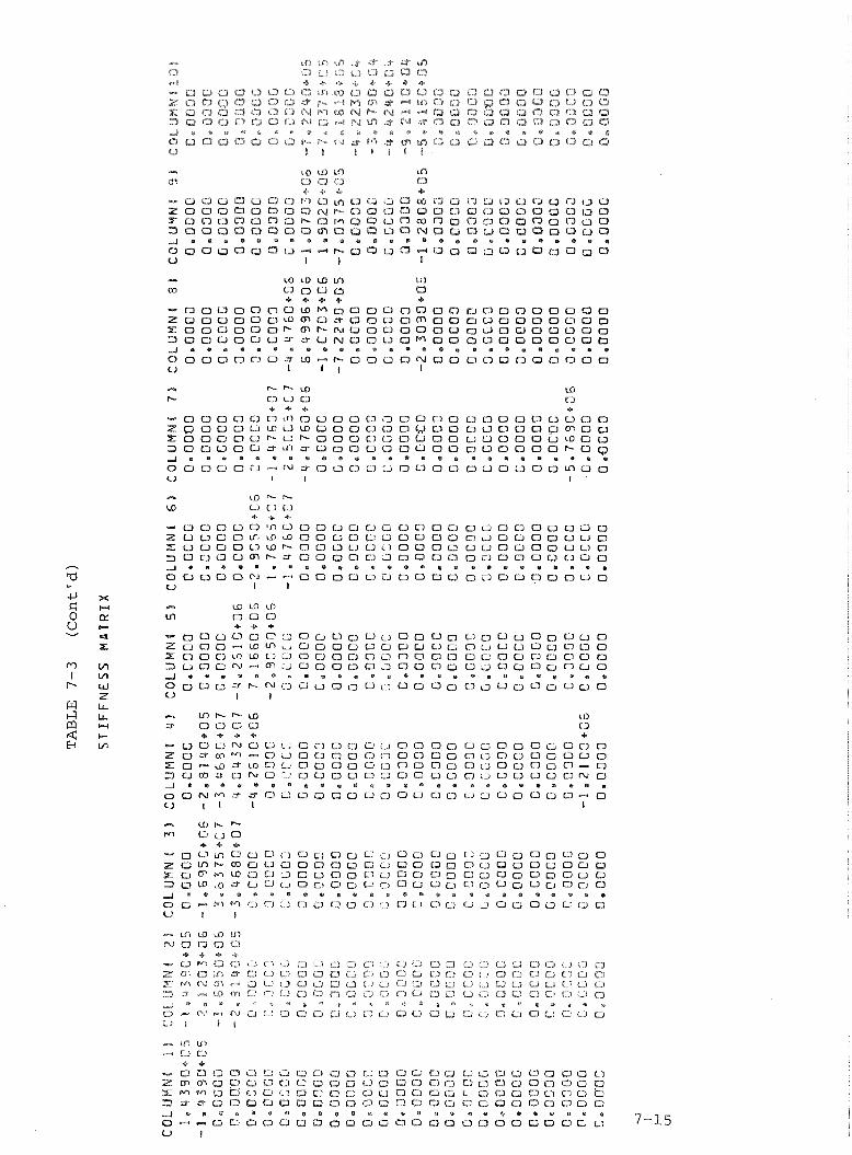
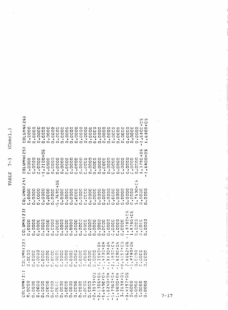
This procedure is exactly the same as that discussed in the four degree-of-freedom system discussed in the previous section.

(:t:;)mii) 3 is equivalent to the A (1,J) matrix discribed in

Appendix 3 (Step 18) and must have nine columns.

The stiffnesses kl and k2 are assumed to have the following mean values and standard deviations.

- kl = 143,900 in-lb.

Okl = .lOkl = 14,390 in-lb. - k2 = 1,695,000 in-lb.

0k2 = .10k2 = 169,500 in-lb.

kl and k2 are also assumed to be statistically independent, The 9 x 9 covariance matrix is as follows:

9 columns -1

The [KR] and [KS] matrix give the row indices and column indices respectively of the rows and columns of the stiffness matrix under consideration. Thus

and

Statistical data were requested for eigenvalues and eigenvectors 2-12 (the first eigenvalue is zero, a rigid body mode) . The statistics of the first four (1-4) and the last four (23- 26) elements of these eigenvectors were requested for computation and printout. The statistical results of the VIDAP run are presented in Tables 7-4, 5, and 6.

Several observations can be made from these results which are significant in the analysis of the statistical characteristics of a system.

The modes which have the greatest uncertainty in the eigenvalue or frequency also have the greatest uncertainty in the eigenvector components, This is substantiated also by an examination of the partial derivatives. Note in Equation (3-30) that the partial. derivative of an eigenvectsr component with respect to a stiffness element contains the expression for the partial derivative of the eigenvalue w i t h respect

t o t h e stiffness. The dependency i s n o t one t o one,

b u t genera l l y an increasc in ahi will lead to an increase i n akrs

(2) Large statistical correlations exist between a11 combinations of eigenvalues and eigenvector components. This indicates that in using the statistical characteristics of the modes and frequencies one must consider covariance.

(3) Percentage variations in modal characteristics are generally smaller than the percentage variations in the stiffnesses. This is not a fixed rule because the uncertainty in the system will grow as more stiffness elements are allowed to become random. However previous observations of various dynamic systems along with the two in this report generally support the trend of modal uncertainty being smaller than stiffness uncertainty.

TABLE 7 -5 Eigenvector Statistics s f the S I1

Longitudinal V i b r a t i o n Model(VIDAB)

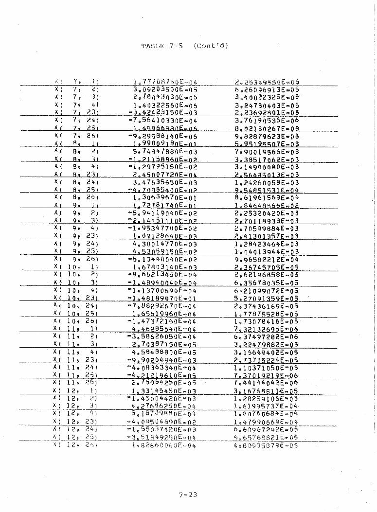
TABLE 7-5 (Cantgd)

LP *P n LCI a m (4 a& 0 o m m Ob)

e .. CPI @ O F

0 00

w or- @ O'P- Q) m m d rnm

0 QC

m Ec- (\I 4- d m (E ( P C

* e c

7 , 3 , 2 Checkout sf VIBAP P a r t i a l Derivatives

W n m b e r sf per tu rba t ion r u n s were made on the S 11 Long i tud ina l V i b r a t i o n model. In each case k l l P kll. k ~ 1 . and k22 in various combinations were perturbed and par t i a derivatives were numerically developed to compare with those computed by VIDAP. Several typical partial derivatives are plotted in Figures 7-6 through 7-15. The partial derivative checks for eigenvalues were excellent, but those for eigenvector components were not altogether satis- factory. It appears that numerical roundoff of the eigenvectors coupled with peculiarities of the problem caused the perturbed model to produce partial derivatives which frequently varied significantly from the VIDAP computed partial derivatives. Basic observations are:

(1) The larger partial derivatives (those which are of the greatest significance) can be computed the most accurately. The smaller partials wander and may even have reversals of sign.

(2) Eigenvectors which have only a few dominant components, such as mode 9, produce reasonably accurate partial derivatives for those components.

The S I1 Longitudinal Vibrational Model appeared to have some peculiarities when perturbed which were difficult to explain. Occasionally adjoining eigenvectors would alter characteristics significantly when the roots became close. The partial derivatives of the first several eigenvectors did not agree at all with the computed partial derivatives. However the small value of these partial derivatives (regardless of accuracy) resulted in small uncertainties for the components and the resulting statistics are of the same small magnitude shown in the Monte Carlo check to be discussed in the next section.

3 -4

P-4 N

X 3 + 4

N F-i

X

d -4

a, tn

0 r= Id C U

4-J d (U U

0 k Ti a, I Pi

0 N I

b

X &) at C U

$ . pl 4-J

s .4 k a, a F-i cd

-rl 4-J k cd Pi

cn I

I-

a, k 3 tr . pl lir

f-i a -4 4J k a, rd 3 PI .ri

c, a a a, 3 4 -4 s k

[" U

+ N N f-i rl

2 I2

0 N

f-i CV

0 X rl

r

N rl

X

C . ri

a, 0 0

C rd c: U

c, C a

0 U f - i k

I a, PC

C3 nJ

I

f-i rl I P

% ry A

4 e, e\d

0 'x

i-i r E -ti

CV 4J i-i ;d

X 3 . fi G k -4 a,

cl a,

0 tr i-i G rd rd . fi s -lJ U k

Id c, PI C

0 CV

i-i CV

X 0 4 4

CV i-i

X

G -ti

at 0 '3

c= rd s U

c, F: at

8 U 4 k

1 Q @4

0 CU

I

m N rl i-i

2 I5 L

'auo oq. ~ewba suoTqepnap pzepueqs PUP SUP~U oxaz Y~TM saIqPTxeA mspuez paqnqTzqsyp K~~ernzow qwapwadapwy ale Zz pwe Iz azayfi

"zy pue Iy sassau33rqs uopuex ayq oq squamaxa xrxqeu ssau33-rqs aqeTax

07 pado~aaap seM uoTqeTax xTxqem bur~o~~o3 ayq '~T-L axnfi-cd ur paqyxasap axnpaaoxd ayq bursn "T*E-L uoTqaaS 30 buruurbaq ayq qe

u~oys sr Zy pue Iy uodn Aauapuadap sq? yqr~ xrxqem ssau33rqs ayL

"1~~3 07 A~ay-g qsom axe suoTqeraap pxepueqs pue sueam anxq ayq y3-r~~ UqqrM sabuex ayq ysrTqeqsa oq papnTauT axe spunoq xo sqyury~ aauapTpoa aauag *saaue?xen pue sueau anxq 30 saqem-gsa

uy sqxnsax A~uo a~dmes aqrurg e 6ursn srsA-pue Tearqsrqeqs Auy

'9 Aq A~exnaae ayq paseaxau? aney ppon S-$SAT~UP unx-09 e aauag =Y/T 30 a282 ayq qe abxanuoa sysA~eue oIxe3 aquom e 30

uo~qe~nap pxepueqs pue ueam paqemrqsa ayq yqoa "samrq OE paqeadax SQM axnpaaoxd ayq s~sd-pue ayq UI "gr-~ axnbsd us mexbe-cp

MOTS ayq u? paqyxasap sy s~sK~eue syyq u~ pasn axnpaaoxd ayL *Tapam TeaTqsTqeqs XesuVC ayq go yaay3 XesTqsTgeqs quapusdspuf

Axa3a%duoa e ZaJJa 03 ST s~sA~eue oaxPa aqwoM s~yq 2s asodxnd ay&

Statistical distribution for each random stiffness: kl and k2

Stiffness matrix a(kllt k12t with vacancies for random a(klr k2, .... )

and compute remaining values in stiffness

Mass matrix and eigenvectors of the system

Output : Summarize and printout mean values and variances of eigenvalues and eigenvectors

Figu re 9-16 S u m a r y of Monte C a r 1 0

Procedure

The r e s u l t s sf the check are s u m a r i z e d in Tables 7-7 and 7-8, Note t h a t the frequency table shaws very excellent correlation between the VIDAP linear statistical mode% and the Monte Carlo, This should be expected since the eigenvalues are relatively well-behaved and the partial derivatives for eigenvabues are simple and are not as easily influenced by accumulative roundoff.

Although Monte Carlo results are not shown for eigenveetor components of modes 2, 3, 4, 6, LO, 11, and 12 it was confirmed that these modes, which have small deviations in the frequencies, also have small deviations in the eigenvector components.

The mean values in Table 7-8 show excellent agreement, but the standard deviations show only fair agreement. However, except in the case of x(5,2), the standard deviations predicted by VIDAP are of the same magnitude. The lack of finer accuracy can be due to the following factors:

(1) nonlinearity in the eigenvector derivatives (2) roundoff error (3) possible unusual behavior of the eigenvectors (4) the limited size of the Monte Carlo.

This project ended before the above areas could be investigated, but the influences of these effects should be thoroughly evaluated before VIDAP is put into general'operation.

Wm

O~

db

mM

OW

Nm

OM

bd

ma

dO

(V

W~

d

~w

Nd

00

4W

00

dd

00

em

bm

~h

lO

OO

m

d0

00

00

0d

w0

00

00

0d

d0

00

OO

O0

.

. I

II

I

I I

II

I

I

nh

hh

h

hC

Ih

.

rl

(4

P9

A

n-

n-

mW

mW

-n

-n

MW

mW

nn

--

MW

mW

d

Nm

WN

NN

Nd

NO

gN

NN

Nd

NM

bl

'N

NN

W

..

..

..

..

..

..

..

..

..

..

..

..

m

mm

mm

mm

mm

mm

aa

wa

aa

mm

Cr

pm

am

a

Vu

VY

Vw

YV

VV

wY

VV

VV

u-

V~

-w

-W

XX

XX

XX

XX

XX

XX

XX

XX

XX

XX

XX

XX

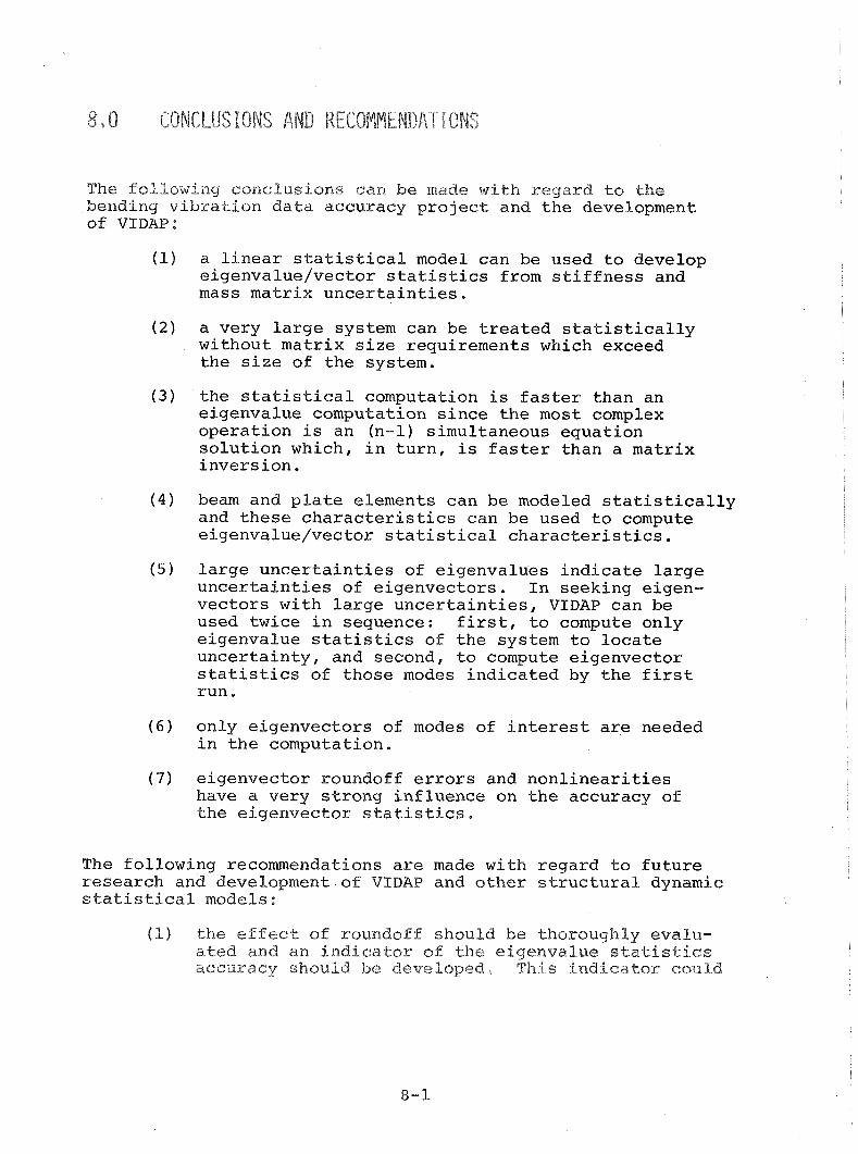
CONCLUS IONS AND REGOMMENBAT1 ONS

The following conclusions can be made with regard to the bending vibration data accuracy project and the development of VIDAP:

(1) a linear statistical model can be used to develop eigenvalue/vector statistics from stiffness and mass matrix uncertainties.

(2) a very large system can be treated statistically without matrix size requirements which exceed the size of the system.

(3) the statistical computation is faster than an eigenvalue computation since the most complex operation is an (n-1) simultaneous equation solution which, in turn, is faster than a matrix inversion.

(4) beam and plate elements can be modeled statistically and these characteristics can be used to compute eigenvalue/vector statistical characteristics.

(5) large uncertainties of eigenvalu'es indicate large uncertainties of eigenvectors. In seeking eigenvectors with large uncertainties, VIDAP can be used twice in sequence: first, to compute only eigenvalue statistics of the system to locate uncertainty, and second, to compute eigenvector statistics of those modes indicated by the first run.

(6) only eigenvectors of modes of interest are needed in the computation.

(7) eigenvector roundoff errors and nonlinearities have a very strong influence on the accuracy of the eigenvector statistics.

The following recommendations are made with regard to future research and development of VIDAP and other structural dynamic statistical models:

(1) the effect of roundoff should be thoroughly evaluated and an indicator sf the eigenvalue statistics accuracy should be developed, T h i s indicator could

OsquamaTa 6uyuroCpe 30 sayqxadoxd ayq uaaMqaq uoyqeTaxxoa Tearqsrqeqs qrmxad 07 pado~aaap aq

pTnoys Tapom y 'pr~ea SA~MTP qou qnq quaruanuoa sy squawaTa aqqd bupqoCpe pue squamaTa meaq 6u~urocpe

30 aauapuadapur Tearqs?qeqs 30 uo-qdwnsse ay& (5)

-sxoqaaauabya ayq 30 sarqsrqeqs ayq Guysn pado~anap aq pTnoqs Tapom asuodsax Tearqsrqeqs y (p)

equear3~ubys sy Aq~xeau?~uou uayM ys-g -qeqsa pTnoM ya~y~ sxoqea~puy SP asn oq pado~anap

aq pTnoys san~eaua6-p ayq 30 san-pen-$xap puoaas (E)

*sqTnsax qsaq 30 uoyqexodxoau~ Aq saarxqeu ssau3grqs 30 quamanoxdmy pug uo~qez%m~qdo se yans suorq-e

--~gdde xayqo 07 sanrqenrxap ~eyqxed dvaIA aqq 30 worqearadde ayq 3s apem aq pxnoys us~qebrqsanw~ uy (z)

a pax~nbax Ksexnsn~ sa aarbap ayq oq slsqsa~uab%a ayq

aqezaqe plnsfi yaTyfi auTgnoxqns e yqy~ papnTDwT sq

REFERENCES

Collins, J. D., and W. T. Thornson, "The Eigenvalue Problem for Structural Systems with Statistical Properties," AIAA Journal, Vol. 7, No. 4, April 1969, pp. 642-648.

Kiefling, Larry A., "Comment on 'The Eigenvalue Problem for Structural Systems with Statistical Properties'", AIAA Journal, July, 1970.

Przemieniechki, J. S., McGraw-Hill Book Company, New York, N. Y. 1968.

Weaver, William, Jr., Computer Programs for Structural Analysis, D. Van Nostrand Company, Inc., Princeton, New Jersey, 1967.

Martin, H. C., "Stiffness Matrix for a Triangular Sandwich Element in Bending," NASA JPL Technical Report No. 32-1158, Jet Propulsion Laboratory, California Insti- tute of Technology, Pasadena, Cal'if. 1967.

Turner, M. J., R. W. Clough, H. C. Martin, and L. J. Topp "Stiffness and Deflection Analysis of Complex ~truc&ures, " Journal of Aeronautical Sciences, Vol. 23, No. 9, pp. 805-823, Sept. 1956.

Rubinstein. Moshe F.. and Richard Rosen, "Structural ~nalGsis by Matrix Decomposition ," Journal of the Franklin Institute, Vol. 286, No. 4, October 1968.

Archer, J. S., "Consistent Mass Matrix for Distributed Mass

f

pp. 161-178, August, 1963.

9. Soong, T. T., and J. L. Bogdanoff, "On the Natural Frequencies of a Disordered Linear Chain of N Degrees of Freedom," International Journal of Mechanical Sciences, Vol. 5,

APPENDIX A

NOMENCLATURE

A.l EIGENVALUE-EIGENVECTOR PARTIAL DERIVATIVE DEVELOPMENT DEFINITIONS

xi - ith eigenvector

x - uth component of ith eigenvector ui equivalent to x(i,u) in computer output

hi - ith eigenvalue

K or [K] - stiffness matrix

krs - (rs) th component of the stiffness matrix

M or [MI - mass matrix

m - (rs) th component of the mass matrix rs

Mi - generalized mass; xit~xi, a scalar quantity

(MT~~) - vector formed from the product Mxi with the uth element removed

the matrix,

- the matrix Fi reduced by removal of the

uth row and uth column.

U - vector of length n-L with zero elements in every location except r where the element is equal to 1, If u i s less than r , the lscatiofl i s at r - l ; and if u = r , the vector is a zero vector ,

axi - a vector sf p a r t i a l derivatives sf the x i

ak,, e igenvec tor w i t h r e s p e c t to the krs element in the stiffness matrix,

a x u i - - t h e uth element of t h e v e c t o r akrs

- u

- t h e v e c t o r reduced by removal of t h e

e lement ,

A.2 COORDINATE DEFINITIONS (SEE FIGURES 4 - 1 and 4 - 4 )

X,, Ym, Zm - s t r u c t u r a l member axes

X,, Y s , Z s - system coord ina t e o r i e n t a t i o n

u i , v i , w i - d e f l e c t i o n s i n t h e member X,, Ym, Z, d i r e c t i o n s r e s p e c t i v e l y a t t h e i node.

0 0 X . 1 - r o t a t i o n s about t h e member X,, Ym axes Yi r e s p e c t i v e l y a t t h e ith node

A.3 GENERAL MATRIX AND VECTOR DEFINITIONS

[ ] - mat r ix

1

- transpose o f a matrix

- a t ~ a t r i x redu d in size by removal of the EE u r o w a n d u column

--"\ vector reduced in s i z e by removal s f the - tth element.

U - a v e c t o r wi th t h e uth element s e t equa l

t o zero

[s] - an upper t r i a n g u l a r mat r ix used i n a decomposition o p e r a t i o n

[DJ - a d iagona l ma t r ix used i n a decomposition ope ra t ion

[KR], [KS] - mat r i ce s of i n d i c e s used t o develop sets of compatible p a r t i a l d e r i v a t i v e s (see Sec t ion 6 . 2 )

A.4 STATISTICAL DEFINITIONS

(-) - mean va lue of ( )

a - s tandard d e v i a t i o n

Cov (xi , x j ) - covar iance of xi and x j

P i j - c o r r e l a t i o n c o e f f i c i e n t s between v a r i a b l e s

Xi and x j

Cov (xi ,x ) P i j =

Ox Ox i j

A . 5 DEFINITIONS USED IN THE DEVELOPMENT OF BEAM AND PLATE STIFFNESS UTRICES

Beam

E - Young's modulus of e l a s t i c i t y

W - Cross-sec t iona l area of a beam element

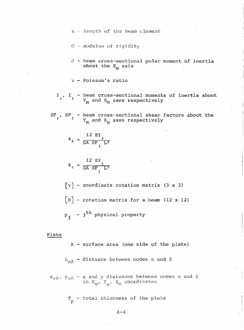
E - l e n g t h of the beam element

G - modulus of r i g i d i t y

J - beam cross-sectional polar moment of inertia about the Xm axis

v - Poisson's ratio

ILt I - beam cross-sectional moments of inertia about

3 Ym and Zm axes respectively

SF3, SF - beam cross-sectional shear factors about the * Ym and Zm axes respectively

12 EI ' = 3 GASF L2

3

12 EI - - 2

'3 GASF L2

[y] - coordinate rotation matrix (3 x 3)

[R] - rotation matrix for a beam (12 x 12)

pj - j th physical property

Plate

A - surface area (one side of the plate)

la^ - distance between nodes a and 6

xu,@, y a , ~ - x and y distances between nodes a and !3 i n Xmr

'rn J

Z, coordinates

T - total thickness of the plate P

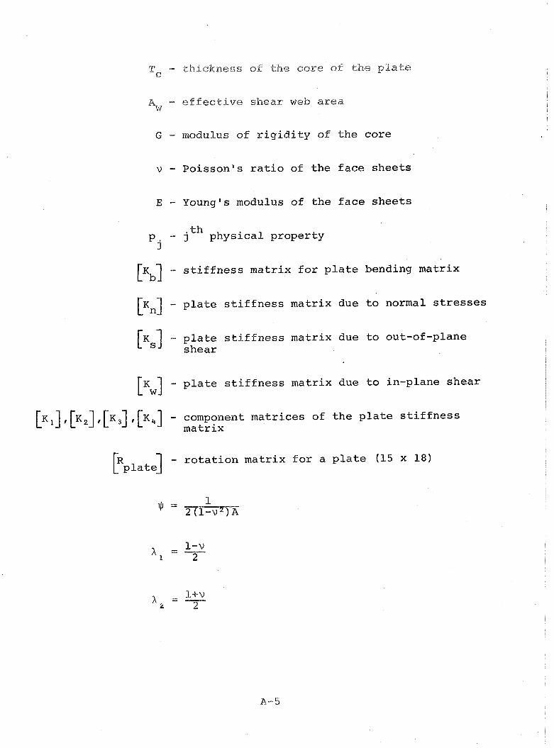
Tc - thickness o f the core of the p la t e

Ww - effective shear w e b area

G - modulus of r i g i d i t y of t h e co re

v - P o i s s o n s s r a t i o of t h e f a c e s h e e t s

E - Young's modulus of t h e f a c e s h e e t s

p - jth p h y s i c a l p rope r ty j

[Xb] - s t i f f n e s s ma t r ix f o r p l a t e bending ma t r ix

[Kn] - p l a t e s t i f f n e s s mat r ix due t o normal stresses

- p l a t e s t i f f n e s s ma t r ix due t o out-of-plane "'l shea r

P W 1 - p l a t e s t i f f n e s s mat r ix due t o in-plane s h e a r

[KI], [K2], [K3] , [K,] - component ma t r i ce s of t h e p l a t e s t i f f n e s s ma t r ix

[R,late] - r o t a t i o n ma t r ix f o r a p l a t e (15 x 18)

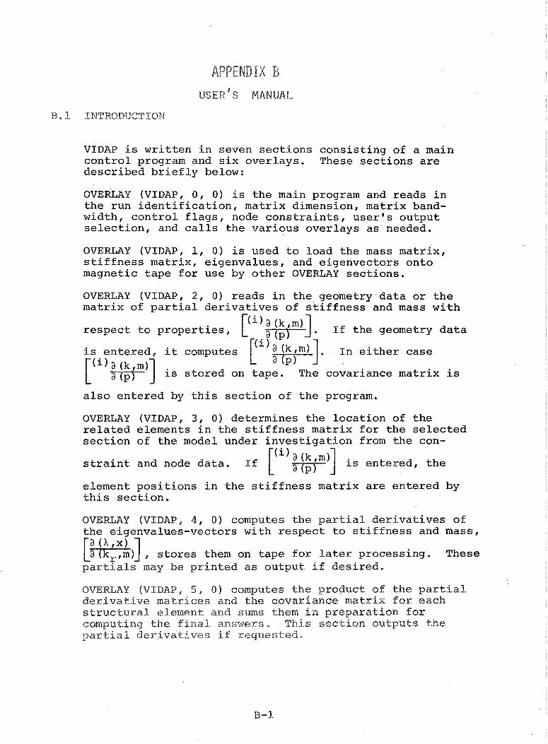
APPENDIX B

E l - 1 INTRODUCTION

VIDAP is written in seven sections consisting of a main control program and six overlays. These sections are described briefly below:

OVERLAY (VIDAP, 0, 0) is the main program and reads in the run identification, matrix dimension, matrix bandwidth, control flags, node constraints, user's output selection, and calls the various overlays as needed.

OVERLAY (VIDAP, 1, 0) is used to load the mass matrix, stiffness matrix, eigenvalues, and eigenvectors onto magnetic tape for use by other OVERLAY sections.

OVERLAY (VIDAP, 2, 0) reads in the geometry data or the matrix of partial derivatives of stiffness and mass with -

respect to properties, If the geometry data

is entered, it computes . In either case

is stored on tape. The covariance matrix is

also entered by this section of the program.

OVERLAY (VIDAP, 3, 0) determines the location of the related elements in the stiffness matrix for the selected section of the model under investigation from the con-

straint and node data. If ) ] is entered, the

element positions in the stiffness matrix are entered by this section.

OVERLAY (VIDAP, 4, 0) computes the partial derivatives of the eigenvalues-vectors with respect to stiffness and mass,

, stores them on tape for later processing. These may be printed as output if desired.

OVERLAY (VPBAP, 5, 0) computes the product of the partial derivative matrices and the covariance matrix for each structural element and sms them in preparation for computing the f i n a l answers, This section outputs the partial derivatives if requested,

OVERLAY (VIDAP, 6 , 0) computes the corre la t ion matrix and s tandard deviations and outputs t h e answers,

IvaaSS AND STIFFNESS m % R E X

The mass and stiffness matrices must be s with a maximum bandwidth of 80 and a maximum dimension of 300. They are entered in a rectangular configuration as shown below:

First column is the matrix diagonal

Data entered & stored in this configuration

CONTROL PUGS

The control flags give the options of: (1) entering the partial derivatives of stiffness and mass with respect to properties or computing these partials, (2) printing-out the partial derivatives of eigenvalues-eigenvectors with respect to stiffness and mass and partial derivatives sf stiffness and mass w i t h respect to proper t i es ,

The node nmber and constraints must be en te red f o r each node having c o n s t r a i n t s , The node numlbers may vary from 1 to 1 0 0 with a m a x i m m of E O O nodes , Each node has s i x degrees of freedom un le s s cons t r a ined . (NOTE: t h e program can handle a maximum of 300 d .0 . f . )

OUTPUT SELECTION

A maximum of 100 elements may be s e l e c t e d f o r t h e ou tpu t . This may be a combination of e igenva lues and s e l e c t e d elements from t h e a s s o c i a t e d e igenvec to r s , o r eigen- va lues a lone . The program checks t o s e e i f t h e mode (1 t o 300) has been reques ted . I f s o , t h e a s s o c i a t e d eigen- va lue becomes one of t h e ou tpu t e lements . The program w i l l then check t h e two s t a r t and s t o p numbers f o r t h e a s s o c i a t e d e igenvec to r . I f t h e f i r s t s t a r t number i s anything o t h e r t han 0 , it w i l l determine t h e s t a r t and s t o p element f o r t h e f i r s t s t r i n g of e igenvec to r e lements a s s o c i a t e d wi th t h i s mode. I t w i l l then check t h e second s t a r t ; and i f it i s n o t 0 , i t w i l l de termine t h e s t a r t and s t o p e lements f o r t h e second s t r i n g of e igenvec tor elements a s s o c i a t e d wi th t h i s mode.

Example :

S t a t i s t i c s a r e d e s i r e d f o r t h e second mode (second e igenva lue) and e lements 1 through 4 and 2 3 through 2 4 . (Note t h a t only two s t r i n g s of cont iguous elements are allowed p e r mode).

The o u t p u t would g ive :

Mode Eigenvalue Standard Deviat ion Freq. S.D.

Vector Eigenvector Standard Deviat ion

INPUT-OUTPUT TAPES

Logical 1, 2, 3 , 4, 9 , and LO are the For t r an tape units required for scratch tapes (binary format), Logical 5 i s t h e i n p u t (card reader) and Logical 6 is the output ( p r i n t e r ) .

B - 2 CARD PREPARqTION

1. Case Heading (I6A5)

This card may contain any alphanmeric character in columns 1-80 for problem identification.

2. N, KBW (218)

Column 1-8 - Integer must.be right justified

N = mass and stiffness matrix dimension, eigenvector length

Column 9-16 - Integer must be right justified

KBW = mass and stiffness matrix bandwidth dimension

3. IFLAG JFLAG (218)

I IFLAG I JFLAG I t

Column 1-8 - Integer must be right justified

IFLAG = 0 = no printout of partial derivatives IFLAG = 1 = printout of all partial derivatives

Column 9-16 - Integer must be rightw justified JFLAG = 0 = compute partial derivatives with

respect to property JFLAG = 1 = input partial derivatives with

respect to property

4. LOT (18)

Column 1-8 - Integer must be right j u s t i f i e d

LOT = node n m b e r o f node w i t h constraints ( k to L O O acceptable)

LOT = 6 or negat ive nmber i s a sentinal to denote t h a t all c o n s t r a i n t s have been entered

5 , KONSTR ( $ ) , , , , , K O N S T R ( 6 1 , ( 6 E 8 ) , ( F o r above node n u d e r )

Column 1-8 - I n t e g e r must be r i g h t j u s t i f i e d

KONSTR = 0 = no c o n s t r a i n t f o r f i r s t d .o . f .* KONSTR = 1 = c o n s t r a i n t f o r f i r s t degree-of-freedom


KONSTR = 0 = no c o n s t r a i n t f o r second d .0 . f . KONSTR = 1 = c o n s t r a i n t f o r second d .0 . f .


KONSTR = 0 = no c o n s t r a i n t f o r t h i r d d .0 . f . KONSTR = 1 = c o n s t r a i n t f o r t h i r d d .0 . f .


KONSTR = 0 = no c o n s t r a i n t f o r f o u r t h d .0 . f . KONSTR = 1 = c o n s t r a i n t f o r f o u r t h d .0 . f .


KONSTR = 0 = no c o n s t r a i n t f o r f i f t h d .0 . f . KONSTR = 1 = c o n s t r a i n t f o r f i f t h d .0 . f .


KONSTR = 0 = no c o n s t r a i n t f o r s i x t h d .0 . f . KONSTR = 1 = c o n s t r a i n t f o r s i x t h d .0 . f .

NOTE: Only LOT (Node Number) and c o n s t r a i n t s f o r LOT need t o be e n t e r e d f o r t hose nodes wi th c o n s t r a i n t s . The program assumes t h a t t h e only nodes wi th con- s t r a i n t s a r e those where c o n s t r a i n t d a t a i s e n t e r e d . I f LOT is ze ro o r nega t ive , t h i s s i g n a l s t h e program t h a t a l l c o n s t r a i n t s have been en t e red . Example: i f t h e system has no c o n s t r a i n t s , only one (1) ca rd would be r equ i r ed : LOT = zero o r nega t ive . LOT (Nodes) must no t exceed one hundred ( 1 0 0 ) i n number o r l e v e l .

*The o r d e r of t h e s i x degrees s f freedom i s a s shown i n F igu re 4 - 1

6, KOBE, RK (218) (Output select cards)

CaPmn 1-8 - I n t e g e r must be r i g h t j u s t i f i e d

KODE = 0 = cont inue to read select va lues KODE = -I - a l l selected mode n u d e r s entered

Column 9-16 - I n t e g e r must be r i g h t justified P

KK = number of mode s e l e c t e d ; i . e . , l = f i r s t mode, 2 = second mode, e t c . KK may vary from 1 t o N (Number of degrees-of-freedom of t h e sys tem) .

Maximum d . 0 . f . accep tab le by t h e program i s 300.

7 . LGO ( I ) , LGO (21, LSTOP ( 1 1 , LSTOP ( 2 ) , (418)

1 8 9 16 17 24 25 32


LGO (1) = number of element f o r s t a r t of f i r s t s e l e c t e d s e c t i o n of v e c t o r ( x )


LGO ( 2 ) = number of element f o r s t a r t of second s e l e c t e d s e c t i o n of v e c t o r (x )


LSTOP (1) = number of element f o r l a s t va lue of f i r s t s e l e c t e d s e c t i o n of v e c t o r (x )


LSTOP (2) = number of element f o r l a s t va lue of second s e l e c t e d s e c t i o n of v e c t o r (x )

The ou tpu t s e l e c t c a r d s e s t a b l i s h t h e amount and o r d e r of p r i n t o u t of t h e e igenva lue and e igenvec tor s t a t i s t i c s as shown i n t h e i n t r o d u c t i o n of t h e appendix. The ou tpu t w i l l always l a b e l t h e s t a t i s t i c a l d a t a b u t does n o t l a b e l t h e p a r t i a l d e r i v a t i v e s which a r e l i s t e d i n t h e ou tpu t as "PARTIAL DERIVATIVES FOR THE EIGENVALUES-EIGENVECTORS (ELEMENT ) . " The o r d e r of t h e s e p a r t i a l d e r i v a t i v e s i n t h e p r i n t = are e s t a b l i s h e d by LGO (1) , LGO ( 2 ) , e t c . and a n example of t h e ou tpu t i s shown below.

Example: LGO (1) = 3 LGO ( 2 ) - 112 LSTOP (1) I= 9 LSTOP (2) = 15

The following data would be saved %or computation of statistics from the p a r t i a l de r iva t ive matrix ( fo r Mode 5):

LGO (2) aX12,5

kll

- partials for consect. eigen- - vector elements x35 through x95

. partials for consect. eigen- . vector elements X12,5 thru X15,5

ESTOP (2) aX15, 5 aX15, 5 . . . . aX15, 5 aX15,5 .. akll 3k12 am11 am2 2

If both LGO's = 0, only the partial derivative of the eigenvalue will be computed and saved (KK).

Once the partials for an eigenvalue and associated eigenvector elements have been listed, the procedure repeats for the next eigenvalue and eigenvector elements as specified by the output select cards.

The order of printout discussed above and demonstrated in the example is also used in the format of the correlation matrix. To demonstrate this consider a very simple output selection such as that below.

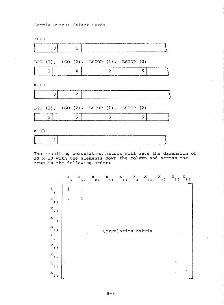
Sample Output Select Cards

KODE

LGO (I), LGO (2), L S T O P (I), L S T O P (2)

KODE

LGO (1), LGO (2), L S T O P (11, L S T O P (2)

KODE

The resulting correlation matrix will have the dimension of 10 x 10 with the elements down the column and across the rows in the following order:

Correlation Matrix

Note that nurntaer in the f i n a l

the eigenvectsr c c q o n e n t s c o n t a i n the mode the second subscript, This order i s reversed i n output, Thus,

eigenvector element n u M e r

mode number

8. M (Mass Matrix Data) (5316.8)

The mass matrix* is entered in the 3 Format with decimal point between columns 4 and 5, 20 and 21, 36 and 37, 52 and 53, and 68 and 69.

Each new row in the matrix must start on a new card.

Example: KBW = 8 (Bandwidth of 8)

Card 1 = 5 values M M M M 11' 12' M13f 14' 15

Card 2 = 3 values M M16f M17' 18'

Blank, Blank

Card 3 = 5 values M M M 22IM23' 24' 25' M26

*The mass matrix must be in consistent units, the geometry data in inches, the stiffness matrix in in-lbs, and the mass will be pounds weight.

9 . K (Stiffness Matrix Data) (5316.8)

Same as Mass Matrix Setup

10. LAMBDA, CODE (2316.8) *

Same Format as 8 and 9

E,P1I\IIBDA = Eigenvalue

CODE = 0 = con t inue

CODE = -I = N o f u r t h e r modes to e n t e r

*See E l , on next page I3-9

Same format and r u l e s as used in 8 and 9

*Data i n s t e p s 1 0 and 11 a r e en t e red i n p a i r s ; i , e , , t h e e igenvaluc and t h e a s s o c i a t e d e igenvec t s r are p a i r e d t o - g e t h e r s e q u e n t i a l l y , No eigenvalue can be en t e red with- o u t an e igenvec tor and v i c e ve r sa .

12. WEIGP ( I ) , WEIG2 (I) , WEIG3 (I) , THE^ ( I ) , THE^ ( I ) , (1) (6F8.0)

3 ca rds r equ i r ed - arranged i n ascending node o r d e r Decimal p o i n t r i g h t j u s t i f i e d u n l e s s e n t e r e d

Column 1-8 * *

W E I G l ( 1 ) = Weight a s s o c i a t e d wi th f i r s t degree-of- freedom of s e l e c t e d element f o r t h e ( 1 ) t h node.

Column 9-16

W E I G 2 ( I ) = Weight a s s o c i a t e d wi th second d . 0 . f .

Column 17-24

WEIG3(I) = Weight a s s o c i a t e d wi th t h i r d d .0 . f .

Column 25-32

T H E l ( 1 ) = Moment of I n e r t i a a s s o c i a t e d wi th f o u r t h d .0 . f .

Column 33-40

THE2(I) = Moment of I n e r t i a a s s o c i a t e d wi th f i f t h d .0 . f .

Column 41-48

THE3(I) = Moment of I n e r t i a a s s o c i a t e d wi th s i x t h d .0 . f .

**Weights a r e e n t e r e d i n pounds and d iv ided by 3 8 6 - 4 w i t h i n t h e program. Moments of i n e r t i a must be en t e red i n terns of mass-in2 where mass is w e i g h t div ided by 3 8 6 - 4 in/sec2,

B-EO

13, COV (5316,8) (See examples in Sect ions 5 and 7 for covariance m a t r i x development)

Same Format as 8

Covariance Matrix ( 9 x 9 )

First card: COVll, COVIZ, COV13, C8V14, COV15 Second card: COV16, COV17, COV18, COV19 Third card: COVZ1, COV22, COV23, COV24, COV25 et cetera

Eighteenth card: COVg6, COVg7, COVg8, COVgg,

14. JNODE, ITYPE, X1, X2, X3 (218, 3F8.0) (3 cards (nodes) required)

Column 1-8 - Integer must be right justified JNODE = Node ID number (Node numbers must be in

ascending order, i.e. JNODE of card 1 < JNODE card 2 < JNODE card 3 )

Column 9-16 - Integer must be right justified ITYPE = 1 - Beam Element ITYPE = 2 - Plate Element

Column 17-24 - Decimal right justified unless punched Xl = Coordinate.value of X for JNODE

Column 25-32 - Decimal right justified unless punched

X2 = Coordinate value of Y for JNODE

Column 33-40 - Decimal right justified unless punched

X3 = Coordinate value of Z for JNODE

15a, Bar Element

E , P R , AREA, X J , X I % , X 1 2 , SF%, SF3 (8P8.0)

Co lmn 1-8 - D e c i m a l right j u s t i f i e d u n l e s s punched.

E = Modulus of e l a s t i c i t y for bar member ,

CoPmn 9-16 - Decimal r i g h t justified unless punched,

PR = Psisssnss r a t i s fo r bar e l emen t ,

C o l m n 17-24 - Decimal right justified u n l e s s punched,

AREA = Cross s e c t i o n a l a r e a of bar .

Column 25-32 - D e c i m a l r i g h t j u s t i f i e d u n l e s s punched.

XJ* = Bar member t o r s i o n a l cons t an t .

*See Sec t ion B . 4 f o r t a b l e of t o r s i o n a l c o n s t a n t s

Column 33-40 - Decimal r i g h t j u s t i f i e d un le s s punched.

X I 1 = Moment of i n e r t i a about t h e Ym a x i s ( ~ i g . 4 - 1 ) .

Column 41-48 - Decimal r i g h t j u s t i f i e d u n l e s s punched.

X I 2 = Moment of i n e r t i a about t h e Zm a x i s (Fig . 4 - 1 ) .


SF2* = Shear shape f a c t o r 2.


SF3* = Shear shape f a c t o r 3.

* Shear shape f a c t o r s f o r bending about t h e Ym and Zm axes a r e given i n Sec t ion 4 . These f a c t o r s , when m u l t i p l i e d by t h e ba r c ros s - sec t ion a r e a , w i l l y i e l d e f f e c t i v e shea r a r e a s f o r t h e member. The pe rmis s ib l e range of SF2 and SF3 is:

. O l 5 SF2 of SF3 5 999.99

15b. P l a t e Element

J l , J 2 , J 3 , TP, E , P R , AW, G (318, SF8.0)

column 1-8 - Integer must be right justified - -

J1 - First. node of p l a t e (nodes must appear in ascending order (i,e, JI < J 2 < 5 3 )

G o l m n 9-16 - I n t e g e r m u s t be right justified

$2 = Second node s f p l a t e ,

Column 17-24 - I n t e g e r m u s t be r i g h t justified

3 3 = Third node of p l a t e

C o l m n 25-32 - Decimal right justified un les s punched

TP = T o t a l t h i c k n e s s of p l a t e

Column 33-40 - Decimal r i g h t j u s t i f i e d u n l e s s punched

E = Modulus of e l a s t i c i t y f o r f a c e s h e e t s


PR = P o i s s o n ' s r a t i o


Core t h i c k n e s s i n i nches


Shear Modulus of c o r e

16a. Bar Element

KEY ( I ) , KEY (2) . - ICEy (8) (818)


K E Y ( 1 ) = S e l e c t e d i n t e g e r from 1 t o 8


KEY(2) = S e l e c t e d i n t e g e r from 1 t o 8

e t c e t e r a

The keys i d e n t i f y t h e independent pa ramete rs t o be random. For a b a r e lement , t h e code i s as fo l l ows :

KEY = 1 KEY = 2 KEY = 3 KEY == 4 KEY =. 5 KEY = 6

KEY = 7

KEY =. 8

Random modulus of e l a s t i c i t y Random c r o s s - s e c t i o n a l a r e a Random moment of i n e r t i a a b s u t t h e Y, a x i s Randsrt~ moment of i n e r t i a about t h e Zm a x i s R a n d o m Poisson" r a t i o Random shear shape fac tor for bending about the Y,, axis Randon! shear shape fac tor f o r bending about t h e Z, a x i s Random b a r meanber t o r s i o n a l c o n s t a n t

Note: Keys do not have to be entered i n sequence ,

Example: D e s i r e Random 1, 4 and 6

16b. P l a t e Element

KEY ( l ) , KEY ( 2 ) , . . KEY ( 5 ) (518)

1 8 9 16 1 7 2 4 25 32 33 40

Column 1-8 I n t e g e r must be r i g h t j u s t i f i e d

KEY(1) - S e l e c t e d i n t e g e r from 1 t o 5

e t c e t e r a

KEY = 1 Random s h e a r modulus KEY = 2 Random s h e a r web c r o s s - s e c t i o n a l a r e a KEY = 3 Random t h i c k n e s s of p l a t e KEY = 4 Random modulus o f e l a s t i c i t y KEY = 5 Random P o i s s o n ' s r a t i o

Note: Keys do n o t have t o be e n t e r e d i n sequence. See example i n 16a.

17 . K I N (18) (Only when JFLAG = 1 and p a r t i a l d e r i v a t i v e s a r e e n t e r e d i n t o t h e program)

1 8

Column 1-8 - I n t e g e r must b e r i g h t j u s t i f i e d

KIN = Number s f r o w s i n t h e p a r t i a l d e r i v a t i v e m a t r i x to be entered Note K I N may not exceed 189

18, A (1,J) jlOP8,O) Partial derivative matrix da ta

Col~aartn 1-8 - D e c i m a l p o i n t r i g h t j u s t i f i e d u n l e s s punched

er of c a r d s A ( 1 , J ) must e q u a l K I N , J may n o t exceed 9 ,

19. LKRS (18) (Only when JFLAG = 1)


LKRS = Dimension of t h e s e l e c t e d KR and KS matrices

LKRS

LKRS

LKRS may n o t exceed 10

20. KR (1018)

1 8 9 16 17

Matr ix w i t h row n er f o r each element

A l l MR = K S ( i , e , d i agona l s t i f f n e s s ma t r i x e lements ) must be on the d iagona l on ly

A11 RR % K S must be in off diagonal locations o n l y

Matrix wi th column number f o r each element

The upper t r i a n g u l a r s e c t i o n w i l l de termine which p a r t i a l d e r i v a t i v e s w i l l be computed.

The p a r t i a l d e r i v a t i v e s f o r each row would be ordered i n t h e p r i n t o u t a s fo l lows:

fol lowed by a / a m ; f o r example

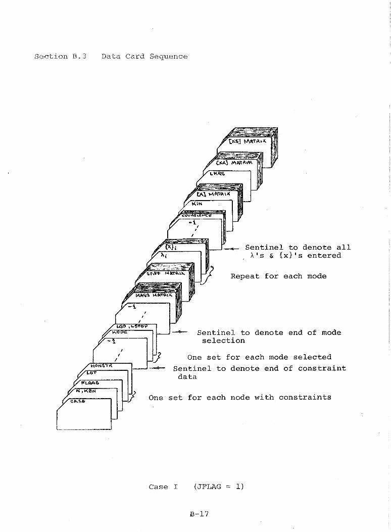
Section B , 3 Data Card Sequence

S e n t i n e l t o denote a l l X's & { X I ' S e n t e r e d

Repeat f o r each mode

S e n t i n e l t o denote end of mode s e l e c t i o n

One s e t f o r each mode s e l e c t e d

S e n t i n e l t o denote end of c o n s t r a i n t

One set f o r each node w i t h c o n s t r a i n t s

Case I ( JPLAG = 1)

B-17

S e n t i n e l o r no more

e lements Repeat f o r e a

One ca rd f o r each node ( 3 c a r d s )

One card f o r each node ( 3 ca rds S e n t i n e l t o denote a l l X ' s &

1x1 ' s e n t e r e d

Repeat f o r each mode

S e n t i n e l t o denote end of s e l e c t d a t a

One s e t f o r each mode s e l e c t e d S e n t i n e l t o denote end of c o n s t r a i n t d a t a

One set f o r each node wi th c o n s t r a i n t s

Case 1% ( J F L A G - 0 )

B-18

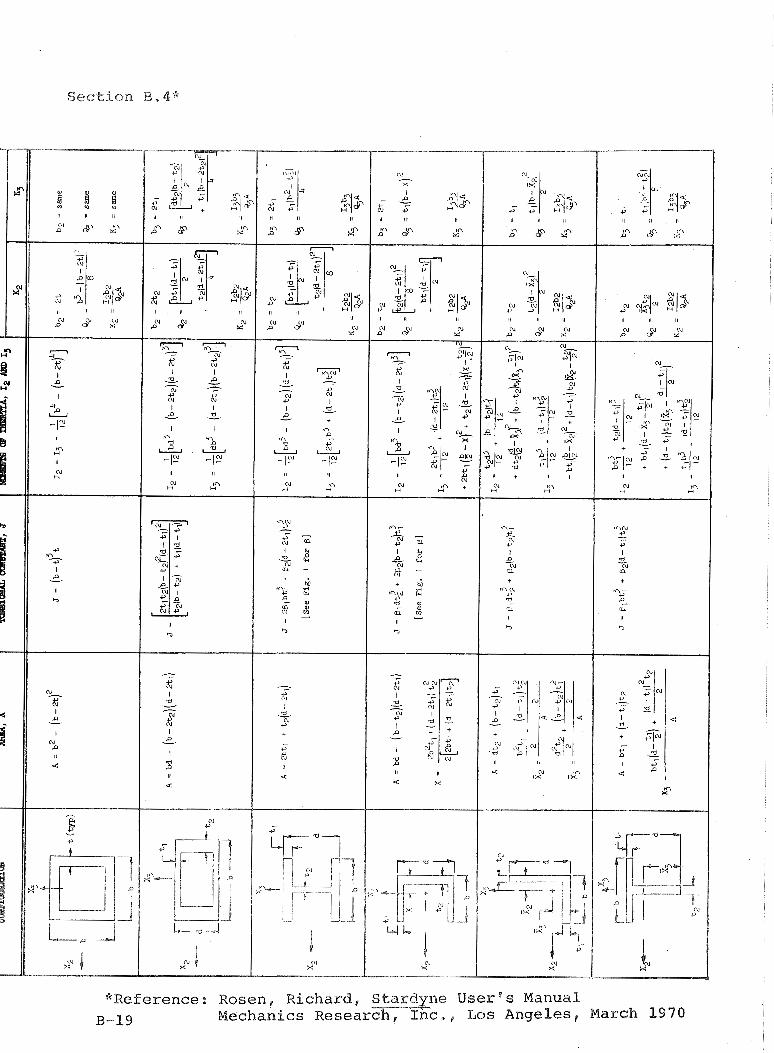
S e c t i o n B,4*

"Reference: Rosen, Richard, Stardyne User's Manual B-19 Mechanics Resear ., LQS Angeles, March 1970

bending vibrational data accuracy … computation speed of the program is less than that required...

Documents