bending, vibration and buckling response...

BENDING, VIBRATION AND BUCKLING RESPONSE OF CONVENTIONAL

AND MODIFIED EULER–BERNOULLI AND TIMOSHENKO BEAM

THEORIES ACCOUNTING FOR THE VON KARMAN GEOMETRIC

NONLINEARITY

A Thesis

by

PATRICK BRIAN MAHAFFEY

Submitted to the Office of Graduate Studies ofTexas A&M University

in partial fulfillment of the requirements for the degree of

MASTER OF SCIENCE

Chair of Committee, J.N. ReddyCommittee Members, Harry Hogan

Miladin RadovicDepartment Head, Andreas Polycarpou

August 2013

Major Subject: Mechanical Engineering

Copyright 2013 Patrick Brian Mahaffey

ABSTRACT

Beams are among the most commonly used structural members that are encoun-

tered in virtually all systems of structural design at various scales. Mathematical

models used to determine the response of beams under external loads are deduced

from the three-dimensional elasticity theory through a series of assumptions con-

cerning the kinematics of deformation and constitutive behavior. The kinematic

assumptions exploit the fact that such structures do not experience significant trans-

verse normal and shear strains and stresses. For example, the solution of the three-

dimensional elasticity problem associated with a straight beam is reformulated as a

one-dimensional problem in terms of displacements whose form is presumed on the

basis of an educated guess concerning the nature of the deformation.

In many cases beam structures are subjected to compressive in-plane loads that

may cause out-of-plane buckling of the beam. Typically, before buckling and during

compression, the beam develops internal axial force that makes the beam stiffer.

In the linear buckling analysis of beams, this internal force is not considered. As

a result the buckling loads predicted by the linear analysis are not accurate. The

present study is motivated by lack of suitable theory and analysis that considers the

nonlinear effects on the buckling response of beams.

This thesis contains three new developments: (1) The conventional beam theories

are generalized by accounting for nonlinear terms arising from εzz and εxz that are

of the same magnitude as the von Karman nonlinear strains appearing in εxx. The

equations of motion associated with the generalized Euler–Bernoulli and Timoshenko

beam theories with the von Karman type geometric nonlinear strains are derived

using Hamilton’s principle. These equations form the basis of investigations to de-

ii

termine certain microstructural length scales on the bending, vibration and buckling

response of beams used in micro- and nano-devices. (2) Analytical solutions of the

conventional Timoshenko beam theory with the von Karman nonlinearity are de-

veloped for the case where the inplane inertia is negligible when compared to other

terms in the equations of motion. Numerical results are presented to bring out the

effect of transverse shear deformation on the buckling response. (3) The development

of a nonlinear finite element model for post-buckling behavior of beams.

iii

To my loving family and friends

for their unending support and encouragement

iv

ACKNOWLEDGEMENTS

I would like to express my gratitude to all of my thesis committee members and

all professors who have helped me succeed during my time as a graduate student.

I extend much appreciation to Dr. Radovic who helped guide me in the field of

mechanical engineering while I was an undergraduate student. He saw an opportunity

to help increase my potential as a young student, and enabled me to obtain a vast

amount of hands-on experience in both materials science and experimental methods

through the design process. His experience and collaboration aided me in receiving

a summer internship that opened my eyes even further to the combined worlds of

science and engineering. This collection of experience, knowledge and guidance has

allowed me to pursue my engineering career even further.

I would also like to specially thank Dr. Reddy. Throughout my graduate school

career he has taught me more than the complex topics covered in his, and other

professors, courses. Allowing me to become one of his research students has enabled

me to broaden my knowledge and understanding of solid mechanics, and has helped

guide me in the direction I am taking to further enrich my career. His constant

devotion to research, education of young minds, and more importantly his patience,

has created an exceptional learning environment and experience that has only en-

couraged me to stay with my work and strive to accomplish great things. Thank you

Dr. Reddy for your guidance, wisdom and willingness to help guide me in the right

direction.

I would like to acknowledge and thank all of Dr. Reddy’s research students who

have helped assist me throughout my graduate studies. Whether it was a simple

homework problem, or a written program that I couldn’t quite figure out, they were

v

always available and willing to lend a hand. A special thanks goes to Mr. Jinseok

Kim and Mr. Venkat Vallala for their help in providing assistance with helping me to

write any MATLAB code that I struggled with. I would also like to specially thank

Mr. Kim for his experience, patience and assistance with other matters concerning

my studies in solid mechanics when I needed additional explaining. Although he was

busy with his own research, he never turned me away when I had a question and

always made extra time to explain details.

I would like to thank my family for their unending encouragement through my

undergraduate and graduate studies. They have always been helpful and stayed

positive even when times were extra stressful. I know I have made them proud and I

would like to continue to do so. A special encouragement goes to my nephew, Ethan.

Although very young right now, I know that he is very intelligent and will go on to do

great things with his life. I would like to use my time here at Texas A&M University,

and my work that has gone into writing this thesis, to help become a positive example

and encourage him to become a successful and professional individual.

Thank you everyone for your continued support.

vi

NOMENCLATURE

σij Stress components in Cartesian coordinates (i, j = 1, 2)

εij Normal strain components in Cartesian coordinates (i, j = 1, 2)

γxz Shear strain component in the x−z plane

θx Slope of the beam in the deformed configuration

φx Rotation of a transverse normal line about the y−axis

∂∂x

Partial derivative with respect to displacement, x

∂∂t

Partial derivative with respect to time, t

δ Variational parameter used in the principle of virtual displacements

δK Virtual kinetic energy

δU Virtual strain energy

δV Virtual external work done

Ks Shear correction factor

λn Eigenvalue for buckling application

Kαβij Stiffness matrix components in Cartesian coordinates (i, j = 1, 2) for

generalized displacements (α, β = 1, 2, 3)

ψi Lagrange interpolation function for virtual axial displacement, δu

ψj Lagrange interpolation function for true axial displacement, u

φi Hermite interpolation function for virtual transverse displacement, δw

φj Hermite interpolation function for true transverse displacement, w

ψ(α)i Lagrange interpolation function (α = 1), Hermite cubic interpolation

function (α = 2, 3) for virtual generalized displacements

ψ(α)j Lagrange interpolation function (α = 1), Hermite cubic interpolation

function (α = 2, 3) for true generalized displacements

vii

TABLE OF CONTENTS

Page

ABSTRACT . . . . . . . . . . . . . . . . . . . . . . . . . . . . . . . . . . . . ii

DEDICATION . . . . . . . . . . . . . . . . . . . . . . . . . . . . . . . . . . . iv

ACKNOWLEDGEMENTS . . . . . . . . . . . . . . . . . . . . . . . . . . . . v

NOMENCLATURE . . . . . . . . . . . . . . . . . . . . . . . . . . . . . . . . vii

TABLE OF CONTENTS . . . . . . . . . . . . . . . . . . . . . . . . . . . . . viii

LIST OF FIGURES . . . . . . . . . . . . . . . . . . . . . . . . . . . . . . . . x

LIST OF TABLES . . . . . . . . . . . . . . . . . . . . . . . . . . . . . . . . . xi

1. INTRODUCTION . . . . . . . . . . . . . . . . . . . . . . . . . . . . . . . 1

1.1 Microstructural Length Scale Studies . . . . . . . . . . . . . . . . . . 11.2 Present Study . . . . . . . . . . . . . . . . . . . . . . . . . . . . . . . 3

2. CONVENTIONAL BEAM THEORIES* . . . . . . . . . . . . . . . . . . . 5

2.1 Conventional Euler–Bernoulli Theory . . . . . . . . . . . . . . . . . . 62.1.1 Equations of Motion . . . . . . . . . . . . . . . . . . . . . . . 8

2.2 Conventional Timoshenko Beam Theory . . . . . . . . . . . . . . . . 102.2.1 Equations of Motion . . . . . . . . . . . . . . . . . . . . . . . 11

2.3 Generalized Force-Displacement Relations . . . . . . . . . . . . . . . 122.4 Static Bending . . . . . . . . . . . . . . . . . . . . . . . . . . . . . . 13

2.4.1 Conventional EBT Model . . . . . . . . . . . . . . . . . . . . 132.4.2 Conventional TBT Model . . . . . . . . . . . . . . . . . . . . 132.4.3 Natural Vibration . . . . . . . . . . . . . . . . . . . . . . . . . 142.4.4 Buckling . . . . . . . . . . . . . . . . . . . . . . . . . . . . . . 15

2.5 Elimination of the Axial Displacement . . . . . . . . . . . . . . . . . 172.5.1 Preliminary Comments . . . . . . . . . . . . . . . . . . . . . . 172.5.2 Conventional EBT . . . . . . . . . . . . . . . . . . . . . . . . 172.5.3 Conventional TBT . . . . . . . . . . . . . . . . . . . . . . . . 20

2.6 Nondimensionalized Governing Equations . . . . . . . . . . . . . . . . 212.6.1 Nondimensional Variables and Parameters . . . . . . . . . . . 212.6.2 Conventional EBT . . . . . . . . . . . . . . . . . . . . . . . . 222.6.3 Conventional TBT . . . . . . . . . . . . . . . . . . . . . . . . 22

2.7 Analytical Solutions for Buckling . . . . . . . . . . . . . . . . . . . . 23

viii

2.7.1 Conventional EBT . . . . . . . . . . . . . . . . . . . . . . . . 232.7.2 Conventional TBT . . . . . . . . . . . . . . . . . . . . . . . . 42

3. MODIFIED BEAM THEORIES* . . . . . . . . . . . . . . . . . . . . . . . 53

3.1 Modified Euler–Bernoulli Theory . . . . . . . . . . . . . . . . . . . . 543.1.1 Equations of Motion . . . . . . . . . . . . . . . . . . . . . . . 54

3.2 Modified Timoshenko Beam Theory . . . . . . . . . . . . . . . . . . . 573.2.1 Displacements and Strains . . . . . . . . . . . . . . . . . . . . 573.2.2 Equations of Motion . . . . . . . . . . . . . . . . . . . . . . . 57

3.3 Generalized Force-Displacement Relations . . . . . . . . . . . . . . . 593.4 Specialization of Equations for Bending, Vibration, and Buckling . . . 60

3.4.1 Static Bending . . . . . . . . . . . . . . . . . . . . . . . . . . 603.4.2 Natural Vibration . . . . . . . . . . . . . . . . . . . . . . . . . 623.4.3 Buckling . . . . . . . . . . . . . . . . . . . . . . . . . . . . . . 63

3.5 Concluding Comments . . . . . . . . . . . . . . . . . . . . . . . . . . 64

4. NONLINEAR FINITE ELEMENT ANALYSIS . . . . . . . . . . . . . . . 65

4.1 Modified Euler–Bernoulli Theory . . . . . . . . . . . . . . . . . . . . 664.2 Modified Timoshenko Theory . . . . . . . . . . . . . . . . . . . . . . 774.3 Results . . . . . . . . . . . . . . . . . . . . . . . . . . . . . . . . . . . 85

5. CONCLUSIONS . . . . . . . . . . . . . . . . . . . . . . . . . . . . . . . . 88

REFERENCES . . . . . . . . . . . . . . . . . . . . . . . . . . . . . . . . . . . 90

APPENDIX A. FULL DERIVATIONS REMOVED FROM THE TEXT . . . 97

ix

LIST OF FIGURES

FIGURE Page

2.1 Kinematics of deformation in the Euler–Bernoulli beam theory. . . . . 7

2.2 Kinematics of deformation in the Timoshenko beam theory. . . . . . . 10

2.3 Buckling of beams with various boundary conditions. . . . . . . . . . 24

2.4 Constant parameter cn vs. applied load for (a) clamped–clampedresults from Nayfeh and Emam (2008), (b) clamped–clamped, (c)hinged–hinged, (d) clamped–hinged and (e) expanded view of clamped–hinged to see remaining bifurcation trends for the present study. . . . 33

2.5 Load–deflection behavior for the first five buckling modes of the clamped–hinged case. . . . . . . . . . . . . . . . . . . . . . . . . . . . . . . . . 35

2.6 Constant parameter cn vs. applied load for hinged–hinged and clamped–clamped boundary conditions for the different aspect ratios. . . . . . 51

x

LIST OF TABLES

TABLE Page

1 Values of the constants ci (i = 1, 2, 3, 4) and eigenvalues λn for buck-ling of beams with various boundary conditions. . . . . . . . . . . . . 32

2 Transverse deflection as a function of loading Λ/π2 and various valuesof ξ for the first buckling mode (λ1 = 4.4943) of the clamped–hinged,conventional EBT beam. . . . . . . . . . . . . . . . . . . . . . . . . . 36

3 Transverse deflection as a function of loading Λ/π2 and various valuesof ξ for the second buckling mode (λ2 = 7.7253) of the clamped–hinged, conventional EBT beam. . . . . . . . . . . . . . . . . . . . . 37

4 Transverse deflection as a function of loading Λ/π2 and various valuesof ξ for the third buckling mode (λ3 = 10.9041) of the clamped–hinged,conventional EBT beam. . . . . . . . . . . . . . . . . . . . . . . . . . 38

5 Transverse deflection as a function of loading Λ/π2 and various valuesof ξ for the fourth buckling mode (λ4 = 14.0662) of the clamped–hinged, conventional EBT beam. . . . . . . . . . . . . . . . . . . . . 39

6 Transverse deflection as a function of loading Λ/π2 and various valuesof ξ for the fifth buckling mode (λ5 = 17.2208) of the clamped–hinged,conventional EBT beam. . . . . . . . . . . . . . . . . . . . . . . . . . 40

7 Values of the constants ci (i = 1, 2, 3, 4) and eigenvalues λn for buck-ling of beams with various boundary conditions for the Timoshenkocase. . . . . . . . . . . . . . . . . . . . . . . . . . . . . . . . . . . . . 48

8 Comparison of λn for the hinged–hinged case for both Euler–Bernoulliand Timoshenko beams. Various aspect ratios (h/l) are given for theTimoshenko theory. . . . . . . . . . . . . . . . . . . . . . . . . . . . . 49

9 Comparison of λn for the clamped–clamped case for both Euler–Bernoulliand Timoshenko beams. Various aspect ratios (h/l) are given for theTimoshenko theory. . . . . . . . . . . . . . . . . . . . . . . . . . . . . 50

10 FEM results for various boundary conditions of conventional EBTmodel; Newton–Raphson iterative process. . . . . . . . . . . . . . . . 87

xi

1. INTRODUCTION

1.1 Microstructural Length Scale Studies

In the last two decades, a number of papers appeared on bringing microstructural

length scales into the continuum description of beams and plates. Eringen’s [1]

nonlocal elasticity is based on the hypothesis that the stress field at a point in an

elastic continuum not only depends on the strain field at the point but also on strains

at all other points of the continuum (i.e., the stress–strain relation is an integral

equation). His observation was based on the atomic theory of lattice dynamics and

experimental observations on phonon dispersion. Eringen converted his nonlocal

integral model to a differential model that contained a single length scale, which was

used by Wang et al. [2], Lu et al. [3], and Reddy and his colleagues [4–10] to bring

out the effect of a single internal characteristic parameter on the bending, buckling,

and vibration characteristics of beams and plates.

Yang et al. [11] developed a modified couple stress theory where the authors

considered an additional energy term due to couple stress tensor in the strain en-

ergy density function. They assumed that the couple stress tensor is related to

the curvature tensor through a single length scale. Such a assumption makes the

analysis simple but it is not a physically realistic assumption because different com-

ponents of couple stress tensor are related, in general, to different components of the

curvature tensor. Microstructure-dependent theories were developed by Park and

Gao [12], [13] for the Bernoulli–Euler beam theory; Ma, Gao, and Reddy [14–16]

for the Timoshenko and Reddy–Levinson beams and Mindlin plates; and Reddy and

his colleagues [17–22], Simisek and Reddy [23], Roque et al. [24], [25], Xia, Wang,

1

and Yin [26], Ke and Wang [27], and Gao, Huang, and Reddy [28] for the first-order

and higher-order beam and plate theories using the modified couple stress theory

proposed by Yang et al. [11].

The nonlocal model of Eringen [1] and the modified couple stress theory of

Yang et al [11] are based on simply postulating the equations directly for small

deformation elasticity, and no attempt was made at a systematic derivation from

finite deformation elasticity. For example, as the modified couple stress theory is

concerned, there is no corresponding finite deformation couple stress theory with

constrained rotations. Recently, Srinivasa and Reddy [29] developed such a finite

deformation gradient elasticity theory for a fully constrained finitely deforming hy-

perelastic cosserat continuum where the directors are constrained to rotate with the

body rotation. This is a generalization of small deformation couple stress theories,

such as the one considered by Yang et al. [11], and it contains several length scales,

the number depending on the type of theory used. The Srinivasa–Reddy finite de-

formation couple stress theory is useful, for example, in modeling an elastic material

with embedded stiff short fibers or inclusions, that is, materials with carbon nan-

otubes or nematic elastomers, cellular materials with oriented hard phases, open cell

foams, and so on.

The commonality between Eringen’s and Yang et al. models is that both bring

a microstructural length scale into the governing equations of a continuum, although

no relationship between the two length scales has been established. Microstructural

length scale can also be brought into the discrete form of structural equations by the

discrete peridynamics approach suggested by Reddy et al. [30]. The approach is yet

to be explored completely.

Another approach through which microstructural length scales can be brought

2

into the structural theory is to account for the additional terms in the strain–

displacement relations. The strain components associated with the simplified Green-

Lagrange strain tensor (see Reddy [31]) E ≈ ε includes small strains but moderately

large rotations, and it is commonly called the von Karman strain tensor, and the as-

sociated theories are termed von Karman beam theories. Conventional von Karman

nonlinear beam theories only account for (1/2)(∂w/∂x)2 in the membrane strain ε(0)xx.

In this study we develop generalized Euler–Bernoulli and Timoshenko beam theories

that account for all terms of the type (1/2)(∂w/∂x)2 in εxx, εzz, and εxz.

1.2 Present Study

In a series of papers, Nayfeh and his colleagues [32–34] claim that they have

obtained the post-buckling configurations of Euler–Bernoulli beams with clamped-

clamped, clamped-hinged and hinged-hinged boundary conditions. They take into

account the von Karman nonlinear strain arising from midplane stretching. They

eliminate the axial displacement from the governing equations under the assumption

that the inplane inertia is negligible and that the ends of the beam are immovable

in the horizontal direction (i.e., the assumption limits application of the resulting

equations only to beams with hinged or fixed ends). Thus, the results they obtained

are not valid for post-buckling response because during post-buckling the ends have

to move due to the applied axial force. Therefore results are applicable only for the

onset of buckling.

In this study, a generalization of the Euler–Bernoulli and Timoshenko beam the-

ories using the simplified Green–Lagrange strain tensor is presented. These theories

bring a couple of microstructural length scales into the beam theories. The theories

are then specialized to conventional theories by omitting the length scale effects. A

3

systematic approach to eliminate the axial displacement for both the Euler–Bernoulli

and Timoshenko beam theories is presented. Analytical solutions for buckling of

beams using the conventional Euler–Bernoulli beams and conventional Timoshenko

beams are presented.

Finally, nonlinear finite element models are developed for the generalized theo-

ries for the buckling application. The primary buckling load is obtained for a variety

of mesh sizes for the conventional and generalized theories of both Euler–Bernoulli

and Timoshenko beams. An initial geometric perfection, of varying magnitude, is

applied to the transverse deflection to initiate buckling instead of just axial displace-

ment while under loading.

4

2. CONVENTIONAL BEAM THEORIES*

The work introduced in this section is reprinted with permission by Ameri-

can Scientific Publishers∗ and covers analytical formulations from Reddy and Ma-

haffey [35]. Several beam theories are applied for research purposes and taught

in the classroom, however, two specific theories are more commonly employed, the

Euler–Bernoulli beam theory (EBT) and the Timoshenko beam theory (TBT). The

Euler–Bernoulli theory is considered the classical beam theory based on the assump-

tions/hypothesis of straight lines normal to the central axis [36], discussed next.

However, the Timoshenko theory, discussed later, relaxes one of the EBT assump-

tions and takes into account a shear correction factor that accounts for the shear

energy present in the beam while undergoing bending [36]. The conventional form

of both theories considers the assumption of inextensible lines normal to the central

axis by removing the Poisson effect, thus neglecting the εzz strain component, which

allows for simpler derivations and the use of one-dimensional constitutive relations

for the principle of virtual generalized displacements and equations of motion. Inde-

pendent of which theory is used to characterize the beam under investigation for an

application, the generalized displacement field, in Cartesian coordinates, is defined

as

u(x, z, t) = u1(x, z, t)e1 + u3(x, z, t)e3 ≡ ux(x, z, t)ex + uz(x, z, t)ez (2.1)

∗Reprinted with permission from J. N. Reddy and P. Mahaffey, “Generalized Beam TheoriesAccounting for von Karman Nonlinear Strains with Application to Buckling,” Journal of CoupledSystems and Multiscale Dynamics, Vol. 1, Copyright [2013] by American Scientific Publishers.

5

which is used to describe displacements in specified directions under kinematic de-

formation. The strain components associated with the simplified Green-Lagrange

strain tensor (E) E ≈ ε includes small strains but moderately large rotations, such

that

Eij ≈ εij =1

2

(∂ui∂xj

+∂uj∂xi

)+

1

2

(∂um∂xi

∂um∂xj

)(2.2)

and it is commonly referred to as the von Karman strain tensor. Conventional von

Karman nonlinear beam theories only account for (1/2)(∂w/∂x)(2) in the membrane

strain ε(0)xx.

We will first discuss the conventional EBT and take a look at the governing

equations of motion which will lead to an analytical solution for the axial buckling

application. Next we will go through the same process and derive the equations of

motion for the conventional Timoshenko case in the same fashion, and present the

differences that lead to a slightly different analytical solution, primarily in the dif-

ferential equation coupling from the transverse displacement and additional rotation

function. Plots and numerical tables will be provided to explicitly show the differ-

ences in buckling modes for both theories, and allow for the deflection–load behavior

for the various boundary conditions of each theory to be observed.

2.1 Conventional Euler–Bernoulli Theory

The conventional EBT, or classical theory, is based on several assumptions con-

cerning straight lines normal to the centerline axis after deformation:

i) rotate as rigid lines to remain normal

ii) no extension in the z-direction (inextensible)

iii) remain straight after deformation.

6

These three assumptions can be seen in Figure 2.1.

Displacements and rotations are exaggerated

z

zw

u

xwx

q¶

=-¶

xxq

xzq

Figure 2.1: Kinematics of deformation in the Euler–Bernoulli beam theory.

The displacement field is given as

ux(x, z, t) = u(x, t) + zθx, uz(x, z, t) = w(x, t), θx ≡ −∂w

∂x(2.3)

with the only strain component present

ε = εxx exex (2.4)

where

εxx = ε(0)xx + zε(1)xx (2.5)

ε(0)xx =∂u

∂x+

1

2

(∂w

∂x

)2

, ε(1)xx =∂θx∂x

(2.6)

For the assumptions stated, we neglect the Poisson effect and transverse shear strain,

such that neither εzz nor γxz = 2εxz are present for the strain field.

7

2.1.1 Equations of Motion

For the governing equations of bending, natural vibrations and buckling due to

an axially applied load, we make use of the principle of virtual displacements. This

is carried out by applying Hamilton’s principle [37] which uses the virtual kinetic

and strain energy, as well as the virtual work done by externally applied forces.

Hamilton’s principle can be expressed as

0 =

∫ t2

t1

(−δK + δU + δV ) dt (2.7)

where δK is the virtual kinetic energy, δU is the virtual strain energy, and δV is the

virtual work done by external forces. The kinetic energy expression is

δK =

∫ l

0

∫A

ρui δui dAdx =

∫ l

0

∫A

ρ[(u+ zθx

)(δu+ zδθx

)+ w δw

]dAdx

=

∫ l

0

[(m0u+m1θx

)δu+

(m1u+m2θx

)δθx +m0 w δw

]dx (2.8)

where

(m0,m1,m2) =

∫A

ρ(1, z, z2)dA (2.9)

and ρ is the mass density.

The expression for the virtual strain energy when the beam is subjected to an

axial compressive force P is

δU =

∫ l

0

∫A

σxx δεxxdAdx− P∫ l

0

∂w

∂x

∂δw

∂xdx+

∫ l

0

Fv δw dx

=

∫ l

0

[M (0)

xx

(∂δu

∂x+∂w

∂x

∂δw

∂x

)+M (1)

xx

∂δθx∂x− P ∂w

∂x

∂δw

∂x+ Fv δw

]dx

(2.10)

where Fv is the viscous force. The viscous force is assumed to be proportional to

8

the velocity w, Fv = µw, where µ is the viscous damping coefficient. Various stress

resultants used in equation (2.10) are defined as

M (0)

xx =

∫A

σxx dA, M (1)

xx =

∫A

z σxx dA (2.11)

where P (∂w/∂x) denotes the component of force along the deformed centerline of

the beam, which is oriented at an angle of ∂w/∂x. The virtual work done by the

external forces is

δV = −∫ l

0

(fx δu+ q δw

)dx (2.12)

where

fx =

∫A

fx dA, q = (qt + qb) (2.13)

and qt and qb denote the distributed load for top and bottom surfaces, respectively,

and fx is the force per unit volume. Substituting δU , δV , and δK into the Hamil-

ton’s principle (2.7), performing integration-by-parts with respect t as well as x to

relieve the generalized displacements δu and δw of any differentiations, and using

the fundamental lemma of calculus of variations, we obtain the following equations

of motion:

−∂M(0)xx

∂x+m0

∂2u

∂t2+m1

∂2θx∂t2

= fx (2.14)

− ∂

∂x

(M (0)

xx

∂w

∂x

)+P

∂2w

∂x2−∂

2M (1)xx

∂x2+m0

∂2w

∂t2+m1

∂3u

∂x∂t2+m2

∂3θx∂t2∂x

+µ∂w

∂t= q (2.15)

with the natural (or force) boundary conditions

δu : M (0)

xx

δw : M (0)

xx

∂w

∂x− P ∂w

∂x+∂M (1)

xx

∂x+m2

∂2θx∂t2

δθx : M (1)

xx

(2.16)

9

2.2 Conventional Timoshenko Beam Theory

The displacement field of the Timoshenko theory relaxes the normality con-

straint of the Euler–Bernoulli theory such that a line normal to the centerline in

the undeformed configuration undergoes additional rotation in the deformed state

such that the angle between the two lines is smaller than 90 degrees, as can be seen

in Figure 2.2. This introduces a new variable φx(x, t) that accounts for the addi-

tional rotation due to shear. This new variable allows us to apply a shear correction

factor [38, 39] when determining the buckling modes, as will be seen in the section

concerning the analytical solution of the buckling application.

This additional rotation combines with θx to develop the shear strain γxz. The

xz x

x

dw

dx

dw

dx

xz

x

dw

dx

z

xw

w

z

Figure 2.2: Kinematics of deformation in the Timoshenko beam theory.

displacement field can be stated as

ux(x, z, t) = u(x, t) + zφx(x, t), uz(x, z, t) = w(x, t) (2.17)

with the strain field

εxx = ε(0)xx + zε(1)xx, γxz = γ(0)

xz (2.18)

ε(0)xx =∂u

∂x+

1

2

(∂w

∂x

)2

, ε(1)xx =∂φx∂x

, γ(0)

xz = φx +∂w

∂x(2.19)

10


Following the same procedure as both forms of the EBT, the equations of motion

for the conventional TBT become

δK =

∫ l

0

∫A

ρuiδui dAdx =

∫ l

0

∫A

ρ[(u+ zφx)(δu+ zδφx) + wδw

]dAdx

=

∫ l

0

[(m0u+m1φx)δu+ (m1u+m2φx)δφx +m0wδw

]dx

(2.19)

where m0, m1 and m2 are defined in Eq. (2.9).

The virtual strain energy δU is computed as

δU =

∫ l

0

∫A

(σxx δεxx + σxz δγxz) dAdx− P∫ l

0

∂w

∂x

∂δw

∂xdx+

∫ l

0

Fv δw dx

=

∫ l

0

[M (0)

xx

(∂δu

∂x+∂w

∂x

∂δw

∂x

)+M (0)

xz

(δφx +

∂δw

∂x

)+M (1)

xx

∂δφx∂x

− P ∂w∂x

∂δw

∂x+ Fvδw

]dx (2.20)

where the stress resultants (M (0)xx and M (1)

xx ) are defined in Eq. (2.11), and we add a

new stress resultant

M (0)

xz =

∫A

σxz dA (2.21)

The expression for the virtual work done by external forces for the TBT case is

the same as in Eq. (2.12), with the exception of the displacement field being applied.

We have

δV = −∫ l

0

(fx δu+ q δw

)dx (2.22)

where (fx, q) are the distributed axial and transverse loads, respectively.

Again, using Hamilton’s principle, we obtain the following equations of motion

11

of the conventional TBT:

− ∂

∂x

(M (0)

xx +M (0)

xz φx

)+m0

∂2u

∂t2+m1

∂2φx∂t2

= fx (2.23)

− ∂

∂x

(M (0)

xz +M (0)

xx

∂w

∂x− P ∂w

∂x

)+ µ

∂w

∂t+m0

∂2w

∂t2= q (2.24)

−∂M(1)xx

∂x+M (0)

xz +m1∂2u

∂t2+m2

∂2φx∂t2

= 0 (2.25)

The natural boundary conditions are

δu : M (0)

xx

δw : M (0)

xz + (M (0)

xx − P )∂w

∂x

δφx : M (1)

xx

(2.26)

2.3 Generalized Force-Displacement Relations

As previously mentioned, for conventional theories we have εzz = 0 and we use

the one-dimensional stress strain relations (i.e., neglecting the Poisson effect, ν = 0)

σxx = Eεxx, σxz = Gγxz (2.27)

Hence the stress resultants are related to the displacements by

M (0)

xx

M (1)xx

M (0)xz

=

∫A

σxx

zσxx

σxz

dA =

A11 ε

(0)xx +B11 ε

(1)xx

B11 ε(0)xx +D11 ε

(1)xx

Axzγ(0)xz

−X (0)

T

X (1)

T

0

(2.28)

12

where

A11 =

∫A

E dA, B11 =

∫A

Ez dA, D11 =

∫A

Ez2 dA,

Axz = Ks

∫A

GdA, X (0)

T =

∫A

E α∆T dA, X (1)

T =

∫A

E z α∆T dA

(2.29)

Here Ks denotes the shear correction coefficient that appears only in the TBT. Note

also that γ(0)xz = 0 for the conventional EBT.

2.4 Static Bending

2.4.1 Conventional EBT Model

For the case of static bending, we omit all terms that contain time derivatives.

The equations for the conventional EBT are

−dM(0)xx

dx=fx (2.30)

−d2M (1)

xx

dx2− d

dx

(M (0)

xx

dw

dx− P dw

dx

)=q (2.31)

where

M (0)

xx = A11

[du

dx+

1

2

(dw

dx

)2]−B11

d2w

dx2−X (0)

T (2.32)

M (1)

xx = B11

[du

dx+

1

2

(dw

dx

)2]−D11

d2w

dx2−X (1)

T (2.33)

2.4.2 Conventional TBT Model

Like the original equations of motion for the TBT case, there are three equa-

tions governing static bending since we must account for the extra rotation variable

13

φx(x, t). This yields the following equations for static bending:

−dM(0)xx

dx= fx (2.34)

− d

dx

(M (0)

xz +M (0)

xx

dw

dx− P dw

dx

)= q (2.35)

−dM(1)xx

dx+M (0)

xz = 0 (2.36)

where

M (0)

xx = A11

[du

dx+

1

2

(dw

dx

)2]

+B11

(dφxdx

)−X (0)

T (2.37)

M (1)

xx = B11

[du

dx+

1

2

(dw

dx

)2]

+D11

(dφxdx

)−X (1)

T (2.38)

M (0)

xz = Axz

(φx +

dw

dx

)(2.39)

2.4.3 Natural Vibration

When dealing with the case of natural vibration for both theories, we set all

externally applied forces except for the axial compressive load P to zero and seek a

solution which is periodic in nature:

u(x, t) = U(x) eiωt, w(x, t) = W (x) eiωt, φx(x, t) = Φ(x) eiωt (2.40)

In addition, we assume that there is no damping (i.e., µ = 0) and we omit thermal

effects. The resulting equations for the various theories are summarized next.

14

2.4.3.1 Conventional EBT

The equations governing natural vibration according to the conventional EBT

are obtained by setting

−ω2(m0U −m1

dW

dx

)− dM (0)

xx

dx= 0 (2.41)

−ω2(m0W +m1

dU

dx−m2

d2W

dx2

)− d2M (1)

xx

dx2− d

dx

[(M (0)

xx − P)dWdx

]= 0 (2.42)

where (M (0)xx and M (1)

xx ) are defined by Eqs. (2.32) and (2.33) in which (u,w, θx) is

replaced by (U,W,−dWdx

).

2.4.3.2 Conventional TBT

For the TBT case, we get:

−ω2 (m0U +m1Φx)−dM (0)

xx

dx= 0 (2.43)

−ω2m0W −d

dx

(M (0)

xx

dW

dx+ M (0)

xz − PdW

dx

)= 0 (2.44)

−ω2 (m1U +m2Φx)−dM (1)

xx

dx+ M (0)

xz = 0 (2.45)

2.4.4 Buckling

In the case of buckling under an axial compressive load P , we set all time deriva-

tive terms and externally applied mechanical and thermal forces to zero to obtain the

governing equations. These are outlined for various theories in the following sections

(one can obtain these equations directly from the governing equations of natural

vibration by omitting the frequency terms). In this section (U,W,Φx) denote the

solutions of the onset of buckling.

15

2.4.4.1 Conventional EBT

For the equations concerning the buckling application, they take the same form

as the equations of bending, with the exception of the applied loading. We are now

only concerned with the axially applied loading P with no transverse loading q and

no fx component. Our buckling equations become

−dM(0)xx

dx= 0 (2.46)

−d2M (1)

xx

dx2− d

dx

[(M (0)

xx − P)dWdx

]= 0 (2.47)

2.4.4.2 Conventional TBT

The equations governing buckling of beams according to the conventional TBT

become:

−dM(0)xx

dx= 0 (2.48)

− d

dx

(M (0)

xx

dW

dx+ M (0)

xz − PdW

dx

)= 0 (2.49)

−dM(1)xx

dx+ M (0)

xz = 0 (2.50)

In the case of beams with material distribution symmetric about the x-axis (i.e.,

Bij = 0 and m1 = 0), the conventional theories can be shown to admit analytical

solutions under certain conditions, as discussed in the next section.

16

2.5 Elimination of the Axial Displacement

2.5.1 Preliminary Comments

In this section we discuss a strategy to eliminate the axial displacement u(x, t)

from the governing equations of motion and absorb the von Karman nonlinear terms

(in terms of the transverse deflection) into a constant. Here we assume that the

beams considered are such that B11 = 0 and m1 = 0. We make the following

assumptions:

(1) There are no thermal effects.

(2) Terms involving the time derivatives such as

m0∂2u

∂t2(2.51)

are very small compared to the rest of the terms in the equation of motion

associated with the x-direction and, therefore, can be neglected.

(3) The beam is supported at x = 0 and x = l such that u(0) = u(l) = 0.

2.5.2 Conventional EBT

For this theory Eqs. (2.14) and (2.15) simplify to

−∂M(0)xx

∂x= fx (2.52)

−∂2M (1)

xx

∂x2−m2

∂4w

∂t2∂x2+m0

∂2w

∂t2+ µ

∂w

∂t− ∂

∂x

(M (0)

xx

∂w

∂x− P ∂w

∂x

)= q (2.53)

17

Integrating Eq. (2.52) with respect to x, we obtain

M (0)

xx +

∫fx dx+ C(t) = 0 (2.54)

or

∂u

∂x+

1

2

(∂w

∂x

)2

+1

A11

[∫fx dx+ C(t)

]= 0 (2.55)

Integrating the above expression from 0 to l and noting that u(0) = u(l) = 0, we

obtain

1

2

∫ l

0

(∂w

∂x

)2

dx+

∫ l

0

[1

A11

∫fx dx

]dx+ SC(t) = 0

or

C(t) = − 1

S

1

2

∫ l

0

(∂w

∂x

)2

dx+

∫ l

0

[1

A11

∫fx dx

]dx

(2.56)

where

S =

∫ l

0

1

A11

dx =l

A11

(2.57)

Note the identity

− ∂

∂x

(M (0)

xx

∂w

∂x

)= −∂M

(0)xx

∂x

∂w

∂x−M (0)

xx

∂2w

∂x2

= fx∂w

∂x+

(∫fx dx

)∂2w

∂x2+ C(t)

∂2w

∂x2(2.58)

where Eqs. (2.52) and (2.54) are utilized in arriving at the second line of Eq. (2.58).

Using Eqs. (2.56) and (2.58) in Eq. (2.53), we arrive at the following equation of

motion governing the transverse displacement w:

m0∂2w

∂t2−m2

∂4w

∂x2∂t2+

∂2

∂x2

(D11

∂2w

∂x2

)+ P

∂2w

∂x2+ µ

∂w

∂t

18

− 1

S

∂2w

∂x2

1

2

∫ l

0

(∂w

∂x

)2

dx+

∫ l

0

1

A11

(∫fx dx

)dx

+fx∂w

∂x+

(∫fx dx

)∂2w

∂x2− q = 0 (2.59)

or

∂2

∂t2

(m0w −m2

∂2w

∂x2

)+

∂2

∂x2

(D11

∂2w

∂x2

)+ P

∂2w

∂x2− q

+µ∂w

∂t− 1

2S

∂2w

∂x2

∫ l

0

(∂w

∂x

)2

dx+

∫ l

0

1

A11

(∫fx dx

)dx

+∂

∂x

[(∫fx dx

)∂w

∂x

]= 0 (2.60)

Equation (2.60) is linear because of the fact

1

2S

[∫ l

0

(∂w

∂x

)2

dx

]

is a constant, which is not known because w is not known.

For the case of free vibrations, Eq. (2.60) reduces to

−ω2

(m0W −m2

d2W

dx2

)+

d2

dx2

(D11

d2W

dx2

)+ P

d2W

dx2+ µiωW

− 1

2S

d2W

dx2

[∫ l

0

(dW

dx

)2

dx

]= 0 (2.61)

For buckling under axial load P , Eq. (2.60) becomes (omitting the damping term)

d2

dx2

(D11

d2W

dx2

)+ P

d2W

dx2− 1

2S

d2W

dx2

[∫ l

0

(dW

dx

)2

dx

]= 0 (2.62)

19

2.5.3 Conventional TBT

For the TBT case, Eqs. (2.23)–(2.25) simplify to

∂M (0)xx

∂x= −fx (2.63)

− ∂

∂x

(M (0)

xz +M (0)

xx

∂w

∂x

)+ P

∂2w

∂x2+ µ

∂w

∂t+m0

∂2w

∂t2= q (2.64)

−∂M(1)xx

∂x+M (0)

xz +m2∂2φx∂t2

= 0 (2.65)

Eqs. (2.54)–(2.58) are also valid for the TBT. Hence, Eqs. (2.64) and (2.65) take

the form

− ∂

∂x

[Axz

(∂w

∂x+ φx

)]− 1

S

∂2w

∂x2

1

2

∫ l

0

(∂w

∂x

)2

dx

+

∫ l

0

1

A11

(∫fx dx

)dx

+ P

∂2w

∂x2+ µ

∂w

∂t− q +m0

∂2w

∂t2

+∂

∂x

[(∫fx dx

)∂w

∂x

]= 0 (2.66)

− ∂

∂x

(D11

∂φx∂x

)+

[Axz

(φx +

∂w

∂x

)]+m2

∂2φx∂t2

= 0 (2.67)

For the free vibration case, Eqs. (2.66) and (2.67) reduce to

−ω2m0W + µiωW − 1

S

d2W

dx2

[1

2

∫ l

0

(dW

dx

)2

dx

]+ P

d2W

dx2

− d

dx

[Axz

(dW

dx+ Φx

)]= 0 (2.68)

−ω2m2Φx −d

dx

(D11

dΦx

dx

)+

[Axz

(dW

dx+ Φx

)]= 0 (2.69)

20

and by omitting the damping term for buckling under axial loading P , we get

Pd2W

dx2− 1

S

d2W

dx2

[1

2

∫ l

0

(dW

dx

)2

dx

]− d

dx

[Axz

(dW

dx+ Φx

)]= 0 (2.70)

− d

dx

(D11

dΦx

dx

)+

[Axz

(dW

dx+ Φx

)]= 0 (2.71)

for both displacements w and φx, respectively.

2.6 Nondimensionalized Governing Equations

2.6.1 Nondimensional Variables and Parameters

We now consider a beam of uniform cross-sectional area A, moment of inertia

I, length l, constant elastic modulus E, and mass density ρ, and is subjected to a

transverse load (fx = 0)

F (0)

z = q = F (x) cosωt (2.72)

This gives us

m0 = ρA, m2 = ρI, A11 = EA, D11 = EI, Axz = GAKs, S =l

EA

Let us introduce the following nondimensional quantities ( [32] and [33]):

ξ =x

l, v =

w

r, ψ =

l

rφx

τ = t1

l2

√EI

ρA, Ω = ω l2

√ρA

EI, r =

√I

A, s2 =

EI

KsGAl2

Λ =Pl2

EI, q =

Fl4

rEI, µ =

µl2√ρEAI

(2.73)

This aides in providing a better general solution that can be applied over a variety

of studies, with the understanding that these variables are used for beams that are

21

considered isotropic.


For this case, Eq. (2.60) takes the form

ρA∂2w

∂t2− ρI ∂4w

∂x2∂t2+ EI

∂4w

∂x4+ P

∂2w

∂x2+ µ

∂w

∂t− F0(x) cosωt

−EA2l

∂2w

∂x2

[∫ l

0

(∂w

∂x

)2

dx

]= 0 (2.74)

which, in terms of the nondimensionalized variables, takes the form (note that ω t =

Ω τ)

∂2v

∂τ 2− r

2

l2∂4v

∂ξ2∂τ 2+∂4v

∂ξ4+Λ

∂2v

∂ξ2+µ

∂v

∂τ− 1

2

∂2v

∂ξ2

[∫ 1

0

(∂v

∂η

)2

dη

]= q(ξ) cos Ωτ (2.75)

for 0 < ξ < 1 and τ > 0.


For the conventional Timoshenko case, Eqs. (2.66) and (2.67) become

∂2v

∂τ 2− 1

s2∂

∂ξ

(∂v

∂ξ+ ψ

)+ µ

∂v

∂τ+ Λ

∂2v

∂ξ2

−1

2

∂2v

∂ξ2

[∫ 1

0

(∂v

∂η

)2

dη

]= q(ξ) cos Ωτ (2.76)

r2

l2∂2ψ

∂τ 2− ∂2ψ

∂ξ2+

1

s2

(∂v

∂ξ+ ψ

)= 0 (2.77)

Thus, one must solve for both v and ψ in the case of the Timoshenko beam theory.

22

2.7 Analytical Solutions for Buckling


2.7.1.1 Governing Equations

For the EBT case of buckling without damping, Eq. (2.75) reduces to

d4v

dξ4+ λ2

d2v

dξ2= 0 (2.78)

where

λ2 = Λ− Γ, Γ =1

2

∫ 1

0

(dv

dη

)2

dη (2.79)

The general solution to Eq. (2.78) for the transverse displacement is [40]

v(ξ) = c1 sinλξ + c2 cosλξ + c3 ξ + c4 (2.80)

where c1, c2, c3, and c4 are constants to be determined using the boundary conditions.

2.7.1.2 Types of Boundary Conditions

The following types of classical boundary conditions are considered first. Note

that for the Euler–Bernoulli beam theory, two boundary conditions at each edge are

required (see Figure 2.3).

Free:

d2v

dξ2= 0,

d3v

dξ3+ λ2

dv

dξ= 0 (2.81)

Hinged:

v = 0,d2v

dξ2= 0 (2.82)

23

Clamped:

v = 0,dv

dξ= 0 (2.83)

Three specific examples, namely, hinged–hinged, clamped–clamped and clamped–

hinged beams are considered next. Note that beams with a free edge cannot be

analyzed because assumption (3) of Section 2.5 is violated.

(b) (c)(a)

z z z

x x x

P P P

ll l

Hinged-Hinged Hinged-Clamped Clamped-Clamped

Figure 2.3: Buckling of beams with various boundary conditions.

2.7.1.3 Hinged–Hinged Beams

For a simply supported beam (at ξ = 0, 1), we have

v = 0,d2v

dξ2= 0 (2.84)

24

Use of the boundary conditions on v gives

v(0) = 0 : c2 + c4 = 0 or c4 = −c2d2v

dξ2

∣∣∣ξ=0

= 0 : − λ2c2 = 0 or c2 = 0

v(1) = 0 : c1 sinλ+ c3 = 0

d2v

dξ2

∣∣∣x=1

= 0 : − λ2c1 sinλ = 0

From the above equations, it follows that

c1 sinλ = 0, c2 = 0, c3 = 0, c4 = 0

The solution for the first constant implies that either c1 = 0 or (and) sinλ = 0. For

a nontrivial solution v, we must have

sinλ = 0 which implies λn =√

Λ− Γ = nπ or n2π2 = Λ− Γ (2.85)

The mode shapes are (c1n = cn)

vn(ξ) = cn sinλnξ, n = 1, 2, 3, · · · (2.86)

where cn is a constant to be determined using the condition

λ2n = Λ− 1

2

∫ 1

0

(dvndη

)2

dη (2.87)

which, for the present case, takes the form

λ2n = Λ− c2nλ2n

2

∫ 1

0

cos2 λnη dη ⇒ cn = ±2

√Λ

λ2n− 1, n = 1, 2, 3, · · · (2.88)

25

where we have used the identity

∫ 1

0

cos2 λnη dη =1

2

∫ 1

0

(1 + cos 2λnη) dη =1

2

[η +

sin 2λnη

λn

]10

=1

2

(1 +

sin 2λnλn

)

and sinλn = 0. Note that vn(ξ) in Eq. (2.86) contains both symmetric (n = 2, 4, · · · )

and unsymmetric (n = 1, 3, · · · ) mode shapes.

2.7.1.4 Clamped–Clamped Beams

For a beam clamped at both ends (at ξ = 0, 1), we have

v = 0,dv

dξ= 0 (2.89)

Use of this set of boundary conditions on v yields

v(0) = 0 : c2 + c4 = 0 or c4 = −c2dv

dξ

∣∣∣ξ=0

= 0 : λc1 + c3 = 0 or c3 = −λc1

v(1) = 0 : c1 sinλ+ c2 cosλ+ c3 + c4 = 0

dv

dξ

∣∣∣ξ=1

= 0 : λ (c1 cosλ− c2 sinλ) + c3 = 0

(2.90)

Using the first two equations, c3 and c4 can be eliminated from the last two equations.

We get

c1 (sinλ− λ) + c2 (cosλ− 1) = 0 and c1 (cosλ− 1)− c2 sinλ = 0 (2.91)

26

For nonzero transverse deflection (i.e., for nonzero values of c1 and c2), we require

that the determinant of the above pair of equations be zero:

∣∣∣∣∣∣∣sinλ− λ cosλ− 1

cosλ− 1 − sinλ

∣∣∣∣∣∣∣ = 0

or

λ sinλ+ 2 cosλ− 2 = 0 (2.92)

This nonlinear (transcendental) equation can be solved by an iterative (Newton’s)

method for various roots of the equation. The first five roots of this equation are

λ1 = 2π, λ2 = 8.9868, λ3 = 4π, λ4 = 15.4505 and λ5 = 6π.

Note that the expression in Eq. (2.92) can be expressed as a product of two

expressions (so that the determination of the roots is made easier) using the identities

cos 2θ = 1− 2 sin2 θ, sin 2θ = 2 sin θ cos θ (2.93)

We obtain

0 = λ sinλ+ 2 cosλ− 2

= 2λ sinλ

2cos

λ

2+ 2− 4 sin2 λ

2− 2

= 4 sinλ

2

(λ

2cos

λ

2− sin

λ

2

)(2.94)

which shows that there are two sets of roots, one corresponding to symmetric modes

sinλ

2= 0 ⇒ λn = 2nπ, n = 1, 2, 3, · · · (2.95)

27

and the other corresponds to unsymmetric modes

tanλ

2=λ

2(2.96)

The mode shapes are determined by using Eqs. (2.80), (2.95), and (2.96). In

particular, we have [c1 is expressed in terms of c2 using the first expression in Eq.

(120)]

c4 = −c2, c3 = −λ c1, c1 =

(1− cosλ

sinλ− λ

)c2 (2.97)

so that we can write

vn(ξ) = c1n sinλnξ + c2n cosλnξ + c3n ξ + c4n

= c1n (sinλnξ − λnξ) + c2n (cosλnξ − 1)

= cn

[1− cosλnξ − (sinλnξ − λnξ)

(1− cosλnsinλn − λn

)](2.98)

where cn = −c2n is a constant to be determined by following the same procedure as

in the case of a hinged–hinged beam. An alternative expression for vn(ξ) is [c2 is

expressed in terms of c1 using the second equation in Eq. (2.91)]

vn(ξ) = cn [1 + cosλn(1− ξ)− λn sinλnξ − cosλnξ − cosλn] (2.99)

where cn = c1n/ sinλn is to be determined.

In view of Eq. (2.98), the symmetric mode shapes are given by (1−cos 2nπ = 0)

vn(ξ) = cn(1− cosλnξ), λn = 2nπ, n = 1, 2, 3, · · · (2.100)

The unsymmetric mode shapes can be determined using Eq. (2.96) and the following

28

identity [where we use Eqs. (2.93) and (2.96)]:

1− cosλ

sinλ− λ=

2 sin2 λ2

2 sin λ2

cos λ2− 2 tan λ

2

=sin λ

2cos λ

2

cos2 λ2− 1

= − cotλ

2= −2

λ(2.101)

Therefore, the mode shapes for unsymmetric case are

vn(ξ) = cn

(1− 2ξ − cosλnξ +

2

λnsinλnξ

)(2.102)

with λn determined from Eq. (2.96).

To determine the constant cn appearing in Eq. (2.98) [the same as that appear-

ing in Eqs. (2.100) and (2.102)], we use the condition in Eq. (2.87) and determine

it with the help of vn(ξ) in Eq. (2.100) (because it is algebraically simpler)


2

∫ 1

0

cos2 λnη dη ⇒ cn = ±2

√Λ

λ2n− 1, n = 1, 2, 3, · · · (2.103)

2.7.1.5 Clamped–Hinged Beams

For a beam clamped at ξ = 0 and hinged at ξ = 1, the boundary conditions

become

At ξ = 0 : v = 0,dv

dξ= 0; At ξ = 1 : v = 0,

d2v

dξ2= 0 (2.104)

29

Use of this combination of boundary conditions on v gives

v(0) = 0 : c2 + c4 = 0 or c4 = −c2dv

dξ

∣∣∣ξ=0

= 0 : λc1 + c3 = 0 or c3 = −λc1

v(1) = 0 : c1 sinλ+ c2 cosλ+ c3 + c4 = 0

d2v

dξ2

∣∣∣ξ=1

= 0 : λ2 (c1 sinλ+ c2 cosλ) = 0

(2.105)

Thus we have c4 = −c3 = −c2 = λ c1, giving the characteristic equation

tanλ− λ = 0 (2.106)

The first five roots of this equation are λ1 = 4.4934, λ2 = 7.7253, λ3 = 10.9041,

λ4 = 14.0662 and λ5 = 17.2208.

The mode shapes for the clamped–hinged beam are


= cn (sinλnξ − λn cosλnξ − λnξ + λn) (2.107)

and the constant cn = c1n is computed from Eq. (2.87) as


2

∫ 1

0

(1 + cos2 λnη + 2λn cosλnη sinλnη − 2λn sinλnη

− 2 cosλnη + λ2n sin2 λnη)dη

cn = ±√

2(Λ− λ2n)

λ2n[2 + λ2n2

+ cosλn(2λn − 12)− 2λn]

, n = 1, 2, 3, · · ·

(2.108)

30

where we have used the following identities

∫ 1

0

cos2 λnη dη =1

2

∫ 1

0

(1 + cos 2λnη) dη =1

2

[η +

sin 2λnη

λn

]10

=1

2

(1 +

sin 2λnλn

),

2λn

∫ 1

0

cosλnηsinλnη dη = λ

∫ 1

0

sin 2λnη dη = −1

2

[cosλnη

]10

= −1

2cosλn +

1

2,

2λn

∫ 1

0

sinλnη dη = −2λn

[cosλnη

]10

= −2λn cosλn + 2λn,

2

∫ 1

0

cosλnη dη = 2

[sinλnη

]10

= 0,

λ2n

∫ 1

0

sin2 λnη dη =λ2n2

∫ 1

0

(1− cos 2λnη) dη =λ2n2

[η − sin 2λnη

2λn

]10

=λ2n2

The relations among the ci for various classical boundary conditions are listed

[taken from [40]] along with the equation governing λn in Table 1. Although clamped–

free and free–free cases are listed in Table 1, they do not correspond to the case in

which the von Karman nonlinearity is included [because assumption (3) of Section

2.5 is violated].

31

Table 1: Values of the constants ci (i = 1, 2, 3, 4) and eigenvalues λn for buckling ofbeams with various boundary conditions.

End conditions at Constants∗ Characteristic equation

ξ = 0 and ξ = 1 and values of λn

Hinged–Hinged c1 6= 0 sinλn = 0, λn = nπ

c2 = c3 = c4 = 0

Clamped–Clamped c1 = (1− cosλn)/(sinλn − λn)c2 λn sinλn + 2 cosλn − 2 = 0

c3 = −λn c1, c4 = −c2 6= 0 λn = 2π, 8.9868, 4π, 15.4505,

6π, · · ·

Clamped–Hinged c1 6= 0 tanλn − λn = 0

c4 = −c3 = −c2 = λ c1 λn = 4.4934, 7.7253, 10.9041,

14.0662, 17.2208 · · ·

Clamped–Free c1 = c3 = 0 cosλn = 0, λn = (2n− 1)π/2

c2 = −c4 6= 0

Free–Free c1 = c3 = 0 sinλn = 0, λn = nπ

c2 6= 0, c4 6= 0

∗ See Eq. (2.80): v(ξ) = c1 sinλξ + c2 cosλξ + c3ξ + c4.

32

0 5 10 15 20−5

−4

−3

−2

−1

0

1

2

3

4

5

Applied Load, Λ/π2

Par

amet

er c

n

Nayfeh and Emam (2008): Clamped−Clamped

P=P2

P=P3

Stableposition

P=P1

Unstableposition

(a)

0 5 10 15 20 25 30 35 40 45−8

−6

−4

−2

0

2

4

6

8


Par

amet

er c

n

Clamped−Clamped

c1(λ

1=2π)

c4(λ

4=15.4505)

c2(λ

2=8.9868)

c3(λ

3=4π)

c5(λ

5=6π)

(b)

0 5 10 15 20 25 30 35

−10

−5

0

5

10

15


Par

amet

er c

n

Hinged−Hinged

c1(λ

1=π)

c3(λ

3=3π)

c5(λ

5=5π)

c2(λ

2=2π)

c4(λ

4=4π)

(c)

0 5 10 15 20 25 30 35 40 45−6

−4

−2

0

2

4

6


Par

amet

er c

n

Clamped−Hinged

c2(λ

2=7.7253)

c3(λ

3=10.9041)

c5(λ

5=17.2208)

c4(λ

4=14.0662)

c1(λ

1=4.4943)

(d)

0 5 10 15 20 25 30 35 40 45−1

−0.8

−0.6

−0.4

−0.2

0

0.2

0.4

0.6

0.8

1


Par

amet

er c

n

Clamped−Hinged (expanded)

c5(λ

5=17.2208)

c2(λ

2=7.7253) c

4(λ

4=14.0662)

c3(λ

3=10.9041)

(e)

Figure 2.4: Constant parameter cn vs. applied load for (a) clamped–clamped re-sults from Nayfeh and Emam (2008), (b) clamped–clamped, (c) hinged–hinged, (d)clamped–hinged and (e) expanded view of clamped–hinged to see remaining bifur-cation trends for the present study.

33

Figure 2.4 depicts the relation between the nondimensionalized applied load

and the constant parameter cn present for each general solution. The constant cn

can be seen as more of an amplitude constant for the transverse deflection vn(ξ).

Due to the quadratic nature of cn, there is zero amplitude for any applied load up

to and equivalent to the analytical buckling load. Any applied load that is larger

than the buckling load allows for a value of cn to be obtained. From the plots,

the bifurcation nature of cn is evident, as seen from the derivations for the various

boundary conditions. The clamped–clamped case in this study is in good agreement

with Nayfeh and Emam (2008), and extends to include the fourth and fifth buckling

modes. The deflection response provides good insight to the postbuckling behavior

as a function of the end constraints.

To see the relationship between the applied load and the transverse deflection

we can take a look at Figure 2.5. For the first five buckling modes of the clamped–

hinged case we can see the transverse deflection of the conventional EBT beam at

various locations along the beam.

34

5 10 15 20 25 30 35 40 45

0

10

20

30

40

50

60

70


Tra

nsve

rse

Def

lect

ion,

v1(ξ

)

Clamped−Hinged, λ1=4.4943

ξ=0.125

ξ=0.75

ξ=1.0

ξ=0.25

ξ=0.875

ξ=0.5

(a)

10 15 20 25 30 35 40 45

−10

−5

0

5

10

15


Tra

nsve

rse

Def

lect

ion,

v2(ξ

)


ξ=0.875ξ=0.75

ξ=1.0

ξ=0.125

ξ=0.5

ξ=0.25

(b)

10 15 20 25 30 35 40 45

−4

−2

0

2

4

6

8

10

12

14

16

18


Tra

nsve

rse

Def

lect

ion,

v3(ξ

)


ξ=0.25

ξ=0.125

ξ=0.875

ξ=0.75

ξ=1.0

ξ=0.5

(c)

15 20 25 30 35 40 45−8

−6

−4

−2

0

2

4

6

8

10

12


Tra

nsve

rse

Def

lect

ion,

v4(ξ

)


ξ=0.5

ξ=0.875

ξ=1.0

ξ=0.75

ξ=0.125ξ=0.25

(d)

20 25 30 35 40 45

−4

−2

0

2

4

6

8


Tra

nsve

rse

Def

lect

ion,

v5(ξ

)


ξ=0.75

ξ=1.0

ξ=0.875

ξ=0.25

ξ=0.125

ξ=0.5

(e)

Figure 2.5: Load–deflection behavior for the first five buckling modes of the clamped–hinged case.

35

As well, some numerical results are presented in Tables 2–6 to explicitly de-

scribe the relation between the applied load, constant parameter cn and transverse

deflection vn(ξ) for the clamped–hinged case of the conventional EBT model:

Table 2: Transverse deflection as a function of loading Λ/π2 and various values of ξfor the first buckling mode (λ1 = 4.4943) of the clamped–hinged, conventional EBTbeam.

v1(ξ)

Λ/π2 c1 ξ = 0.125 ξ = 0.25 ξ = 0.5 ξ = 0.75 ξ = 0.875 ξ = 1.0

4.4943 0 0 0 0 0 0 0

5 0.6108 0.4042 1.4225 3.5674 3.2211 1.8393 0

7.5 1.6738 1.1075 3.8979 9.7754 8.8264 5.0401 0

10 2.4903 1.6477 5.7993 14.5439 13.1320 7.4986 0

12.5 3.2516 2.1515 7.5722 18.9901 17.1466 9.7910 0

15 3.9894 2.6397 9.2905 23.2992 21.0374 12.0127 0

17.5 4.7148 3.1197 10.9797 27.5358 24.8627 14.1970 0

20 5.4328 3.5947 12.6517 31.7288 28.6486 16.3589 0

22.5 6.1459 4.0665 14.3124 35.8935 32.4091 18.5062 0

25 6.8557 4.5362 15.9653 40.0388 36.1520 20.6435 0

27.5 7.5631 5.0042 17.6126 44.1702 39.8823 22.7735 0

30 8.2687 5.4711 19.2559 48.2911 43.6032 24.8982 0

32.5 8.9730 5.9371 20.8959 52.4042 47.3169 27.0188 0

35 9.6762 6.4024 22.5335 56.5110 51.0250 29.1363 0

37.5 10.3785 6.8671 24.1691 60.6129 54.7287 31.2511 0

40 11.0802 7.3314 25.8031 64.7107 58.4288 33.3639 0

42.5 11.7813 7.7953 27.4358 68.8053 62.1259 35.4751 0

45 12.4819 8.2589 29.0674 72.8972 65.8205 37.5848 0

36

Table 3: Transverse deflection as a function of loading Λ/π2 and various values ofξ for the second buckling mode (λ2 = 7.7253) of the clamped–hinged, conventionalEBT beam.

v2(ξ)

Λ/π2 c2 ξ = 0.125 ξ = 0.25 ξ = 0.5 ξ = 0.75 ξ = 0.875 ξ = 1.0

7.7253 0 0 0 0 0 0 0

10 0.2717 0.8659 2.5686 2.4464 -1.4555 -1.4780 0

12.5 0.4204 1.3401 3.9752 3.7860 -2.2526 -2.2874 0

15 0.5501 1.7534 5.2011 4.9536 -2.9473 -2.9929 0

17.5 0.6718 2.1413 6.3519 6.0497 -3.5994 -3.6551 0

20 0.7893 2.5157 7.4624 7.1073 -4.2287 -4.2941 0

22.5 0.9041 2.8817 8.5483 8.1415 -4.8440 -4.9189 0

25 1.0172 3.2423 9.6180 9.1603 -5.4501 -5.5344 0

27.5 1.1292 3.5991 10.6763 10.1682 -6.0498 -6.1434 0

30 1.2402 3.9530 11.7262 11.1682 -6.6448 -6.7476 0

32.5 1.3506 4.3049 12.7700 12.1623 -7.2363 -7.3482 0

35 1.4605 4.6551 13.8089 13.1518 -7.8250 -7.9460 0

37.5 1.5700 5.0041 14.8440 14.1376 -8.4115 -8.5416 0

40 1.6791 5.3520 15.8760 15.1205 -8.9964 -9.1355 0

42.5 1.7880 5.6990 16.9056 16.1011 -9.5798 -9.7279 0

45 1.8967 6.0454 17.9330 17.0796 -10.1620 -10.3191 0

37

Table 4: Transverse deflection as a function of loading Λ/π2 and various values ofξ for the third buckling mode (λ3 = 10.9041) of the clamped–hinged, conventionalEBT beam.

v3(ξ)

Λ/π2 c3 ξ = 0.125 ξ = 0.25 ξ = 0.5 ξ = 0.75 ξ = 0.875 ξ = 1.0

10.9041 0 0 0 0 0 0 0

12.5 0.1291 1.0677 2.3958 -0.3404 0.9226 1.5592 0

15 0.2176 1.7995 4.0380 -0.5737 1.5550 2.6279 0

17.5 0.2891 2.3912 5.3658 -0.7623 2.0663 3.4921 0

20 0.3542 2.9291 6.5726 -0.9337 2.5310 4.2775 0

22.5 0.4158 3.4383 7.7155 -1.0961 2.9711 5.0212 0

25 0.4752 3.9302 8.8192 -1.2529 3.3961 5.7395 0

27.5 0.5333 4.4105 9.8969 -1.4060 3.8112 6.4409 0

30 0.5904 4.8826 10.9563 -1.5565 4.2191 7.1303 0

32.5 0.6467 5.3487 12.0022 -1.7051 4.6219 7.8110 0

35 0.7026 5.8102 13.0379 -1.8522 5.0207 8.4850 0

37.5 0.7579 6.2682 14.0656 -1.9982 5.4165 9.1539 0

40 0.8130 6.7234 15.0870 -2.1433 5.8098 9.8186 0

42.5 0.8677 7.1763 16.1032 -2.2877 6.2011 10.4799 0

45 0.9223 7.6273 17.1152 -2.4315 6.5908 11.1386 0

38

Table 5: Transverse deflection as a function of loading Λ/π2 and various values ofξ for the fourth buckling mode (λ4 = 14.0662) of the clamped–hinged, conventionalEBT beam.

v4(ξ)

Λ/π2 c4 ξ = 0.125 ξ = 0.25 ξ = 0.5 ξ = 0.75 ξ = 0.875 ξ = 1.0

14.0662 0 0 0 0 0 0 0

15 0.0606 0.9640 1.4099 -0.1562 0.5259 -0.7328 0

17.5 0.1211 1.9264 2.8174 -0.3121 1.0510 -1.4644 0

20 0.1653 2.6307 3.8475 -0.4262 1.4352 -1.9999 0

22.5 0.2042 3.2493 4.7523 -0.5265 1.7727 -2.4701 0

25 0.2403 3.8241 5.5930 -0.6196 2.0863 -2.9071 0

27.5 0.2748 4.3723 6.3948 -0.7084 2.3854 -3.3238 0

30 0.3081 4.9029 7.1708 -0.7944 2.6748 -3.7272 0

32.5 0.3407 5.4211 7.9286 -0.8784 2.9575 -4.1211 0

35 0.3727 5.9300 8.6730 -0.9608 3.2352 -4.5080 0

37.5 0.4042 6.4320 9.4072 -1.0422 3.5090 -4.8896 0

40 0.4354 6.9285 10.1333 -1.1226 3.7799 -5.2670 0

42.5 0.4663 7.4206 10.8530 -1.2024 4.0484 -5.6411 0

45 0.4971 7.9091 11.5676 -1.2815 4.3149 -6.0125 0

39

Table 6: Transverse deflection as a function of loading Λ/π2 and various values ofξ for the fifth buckling mode (λ5 = 17.2208) of the clamped–hinged, conventionalEBT beam.

v5(ξ)

Λ/π2 c5 ξ = 0.125 ξ = 0.25 ξ = 0.5 ξ = 0.75 ξ = 0.875 ξ = 1.0

17.2208 0 0 0 0 0 0 0

17.5 0.0240 0.6078 0.4509 0.5069 -0.2764 0.3969 0

20 0.0783 1.9855 1.4729 1.6560 -0.9028 1.2966 0

22.5 0.1114 2.8270 2.0970 2.3577 -1.2854 1.8460 0

25 0.1395 3.5380 2.6245 2.9508 -1.6087 2.3103 0

27.5 0.1650 4.1856 3.1049 3.4909 -1.9031 2.7332 0

30 0.1890 4.7956 3.5574 3.9997 -2.1805 3.1316 0

32.5 0.2121 5.3808 3.9915 4.4877 -2.4465 3.5137 0

35 0.2345 5.9485 4.4126 4.9611 -2.7047 3.8844 0

37.5 0.2564 6.5032 4.8241 5.4238 -2.9569 4.2466 0

40 0.2778 7.0481 5.2283 5.8783 -3.2046 4.6024 0

42.5 0.2990 7.5853 5.6268 6.3263 -3.4489 4.9532 0

45 0.3200 8.1162 6.0206 6.7691 -3.6903 5.2999 0

2.7.1.6 Other Boundary Conditions

Some non-classical boundary conditions that have not been studied in the liter-

ature are listed next.

Elastically Hinged:

v + α

(d3v

dξ3+ λ2

dv

dξ

)= 0,

d2v

dξ2= 0 (2.109)

where α is the inverse of a nondimensional elastic (spring) constant. When α = 0

40

(i.e., the support is rigid), we recover the conventional simply supported boundary

condition. When α is very large, the boundary condition approaches that of a free

edge.

For the case of α = 0 (or as α approaches 0), the boundary conditions become

that of the clamped–hinged case from the previous section, with the constants cn

being the same. However, as α increases the beam takes on the boundary conditions

of a clamped–free system. With the constants c1 = c3 = 0, c2 = −c4 6= 0, the mode

shapes become


= cn(cosλnξ − 1)

(2.110)

and the constant cn is computed as


2

∫ 1

0

sin2 λnη dη ⇒ cn = ±2

√Λ

λ2n− 1 , n = 1, 2, 3, · · · (2.111)

Elastically Clamped:

v = 0,dv

dξ+ β

d2v

dξ2= 0 (2.112)

where β is the inverse of the torsional spring constant. When β = 0 (i.e., the restraint

is rigid), we recover the conventional clamped boundary condition. This gives us a

clamped–clamped system with the same mode shapes vn(ξ) and constants cn given

in Section 2.7.1.4.

On the other hand, if β is very large (i.e., the restraint is very flexible), the con-

dition approaches that of a simply supported case which makes use of the boundary

conditions for a clamped–hinged system. This form of an elastically clamped beam

41

will yield the same mode shapes vn(ξ) and constants cn as those in Section 2.7.1.5.


For the TBT case, Eq. (2.76) and (2.77) give us the pair of second-order coupled

differential equations:

− 1

s2

(d2v

dξ2+dψ

dξ

)+ Λ

d2v

dξ2− 1

2

d2v

dξ2

[∫ 1

0

(dv

dη

)2

dη

]= 0

−d2ψ

dξ2+

1

s2

(dv

dξ+ ψ

)= 0

or

− 1

s2dψ

dξ− λ2s

d2v

dξ2= 0 (2.113)

−d2ψ

dξ2+

1

s2

(dv

dξ+ ψ

)= 0 (2.114)

where

λ2s =1

s2+ Γ− Λ =

1

s2− λ2 , Γ =

1

2

[∫ 1

0

(dv

dη

)2

dη

],

1

s2=GAKsl

2

EI(2.115)

For a rectangular cross-section beam with height h width b, and length l, we have

s2 =1 + ν

5

(h

l

)2

= 0.26

(h

l

)2

for ν = 0.3 (2.116)

Solving Eq. (2.113) for dψ/dξ,

dψ

dξ= −s2λ2s

d2v

dξ2

42

and substituting the result into Eq. (2.114) (after differentiating it once), we obtain

s2λ2sd4v

dξ4+ λ2

d2v

dξ2= 0 or

d4v

dξ4+ β2d

2v

dξ2= 0 (2.117)

where

β2 =λ2

s2λ2s=

λ2

1− s2λ2or λ2 =

β2

1 + s2β2(2.118)

The general solution to this equation is of the form

v(ξ) = c1 sin βξ + c2 cos βξ + c3ξ + c4 (2.119)

The solutions for the TBT can be obtained in the same manner as the EBT so-

lutions for the various boundary conditions using the general solution in Eq. (2.119).

The solutions are discussed here for the same various boundary conditions.

2.7.2.1 Hinged–Hinged Beams

Using the boundary conditions we obtain

v(0) = 0 : c2 + c4 = 0 or c2 = −c4dψ

dξ

∣∣∣ξ=0

= 0⇒ d2v

dξ2

∣∣∣ξ=0

= 0 : c2 = c4 = 0

v(1) = 0 : c1 sin β + c3 = 0

d2v

dξ2

∣∣∣x=1

= 0 : c1 sin β = 0⇒ c3 = 0

From the above equations, it follows from Eq. (2.118) that

sin β = 0 → βn = nπ or λ2n =β2n

1 + s2β2n

(2.120)

43

Thus we have

λ2n =n2π2

1 + n2π2 s2= Λ− Γ (2.121)

The mode shapes are

vn(ξ) = cn sin βnξ, n = 1, 2, 3, · · · (2.122)

where cn is given by

cn = ±2

√Λ

λ2n− 1, n = 1, 2, 3, · · · (2.123)

2.7.2.2 Clamped–Clamped Beams

For a beam clamped at both ends (at ξ = 0, 1), we have

v = 0, ψ = 0 at ξ = 0, 1 (2.124)

In order to use the boundary conditions on ψ, we note the following relationship

[see [41], p. 196]

ψ(ξ) = −s2λ2sdv

dξ− s2λ2c3 (2.125)

Use of the boundary conditions gives

v(0) = 0 : c2 + c4 = 0 or c4 = −c2

ψ(0) = 0 : s2λ2sβc1 + c3 = 0 or c3 = −s2λ2sβc1

v(1) = 0 : c1 sin β + c2 cos β + c3 + c4 = 0

ψ(1) = 0 : s2λ2sβ (c1 cos β − c2 sin β) + c3 = 0

44

Using the first two equations, c3 and c4 can be eliminated from the last two equations.

We have

c1(sin β − s2λ2sβ

)+ c2 (cos β − 1) = 0 and c1 (cos β − 1)− c2 sin β = 0 (2.126)

For nonzero transverse deflection (i.e., for nonzero values of c1 and c2), we require

that the determinant of the above pair of equations be zero:

∣∣∣∣∣∣∣sin β − s2λ2sβ cos β − 1

cos β − 1 − sin β

∣∣∣∣∣∣∣ = 0

or

s2λ2s β sin β + 2 cos β − 2 = 0 (2.127)

This transcendental equation takes the same form as Eq. (2.92) and must also be

solved iteratively for the proper values of βn which can then be used to determine the

corresponding values of λn. Using the same method and identities from Eq. (2.93)

and (2.94), we have

0 = s2λ2sβ sin β + 2 cos β − 2

= 2s2λ2sβ sinβ

2cos

β

2+ 2− 4 sin2 β

2− 2

= 4 sinβ

2

(s2λ2sβ

2cos

β

2− sin

β

2

)(2.128)

which shows that there are two sets of roots, one corresponding to symmetric modes

sinβ

2= 0 ⇒ β = 2nπ, n = 1, 2, 3, · · · (2.129)

45

and the other corresponds to unsymmetric modes

tanβ

2=s2λ2sβ

2(2.130)

Applying the constants obtained from the boundary conditions and

c1 =

(1− cos β

sin β − s2λ2sβ

)c2 (2.131)

we can obtain the general solution as

vn(ξ) = c1n sin βnξ + c2n cos βnξ + c3n ξ + c4n

= c1n(sin βnξ − s2λ2sβnξ

)+ c2n (cos βnξ − 1)

= cn

[1− cos βnξ −

(sin βnξ − s2λ2sβnξ

)( 1− cos βnsin βn − s2λ2sβn

)](2.132)

The alternative expression for vn(ξ) is [c2 is expressed in terms of c1 using the second

equation in Eq. (2.126)]

vn(ξ) = cn[1 + cos βn(1− ξ)− s2λ2sβn sin βnξ − cos βnξ − cos βn

](2.133)

where cn = c1n/ sin βn is to be determined.

In view of Eq. (2.132), the symmetric mode shapes are given by (1−cos 2nπ = 0)

vn(ξ) = cn(1− cos βnξ), βn = 2nπ, n = 1, 2, 3, · · · (2.134)

The unsymmetric mode shapes can be determined using Eq. (2.130) and the following

46

identity [where we use Eqs. (2.93) and (2.130)]:

1− cos β

sin β − s2λ2sβ=

2 sin2 β2

2 sin β2

cos β2− 2 tan β

2

=sin β

2cos β

2

cos2 β2− 1

= − cotβ

2= − 2

β(2.135)

Therefore the mode shapes for the unsymmetric case are

vn(ξ) = cn

(1− 2s2λ2sξ − cos βnξ +

2

βnsin βnξ

)(2.136)

with λn determined from Eq. (2.133).

Since this follows so closely to the clamped–clamped case for the EBT, we can

use the form applied to obtain cn in Eq. (2.103) for the TBT case, so that

cn = ±2

√Λ

λ2n− 1, n = 1, 2, 3, · · · (2.137)

In Table 7 the constants cn as well as the characteristic equation and respective

eigenvalues λn associated with the different boundary conditions are presented for the

conventional Timoshenko case. As well, Tables 8 and 9 compare the Euler–Bernoulli

and Timoshenko buckling modes for the hinged–hinged and clamped–clamped cases,

respectively. The Timoshenko results are dependent upon the aspect ratio, as can

be seen in the columns presented.

47

Table 7: Values of the constants ci (i = 1, 2, 3, 4) and eigenvalues λn for buckling ofbeams with various boundary conditions for the Timoshenko case.

End conditions at Constants∗ Characteristic equation

ξ = 0 and ξ = 1 and values of λn

Hinged–Hinged c1 6= 0 sinβn = 0 ⇒ βn = nπ

c2 = c3 = c4 = 0 λn = βn√1+β2

ns2

Clamped–Clamped∗∗ c1 = (1− cosβn)/(sinβn − s2λ2sβn)c2 s2λ2sβn sinβn + 2 cosβn − 2 = 0

c3 = −s2λ2sβn c1, c4 = −c2 6= 0 λn = βn√1+β2

ns2

∗ See Eq. (2.119): v(ξ) = c1 sinβξ + c2 cosβξ + c3ξ + c4.

∗∗ βn must be determined by solving the transcendental equation.

48

Table 8: Comparison of λn for the hinged–hinged case for both Euler–Bernoulli andTimoshenko beams. Various aspect ratios (h/l) are given for the Timoshenko theory.

TBT

Mode EBT h/l = 0.001 h/l = 0.01 h/l = 0.05 h/l = 0.1

1 3.14159 3.14159 3.14119 3.13156 3.10204

2 6.28319 6.28315 6.279963 6.204089 5.9836

3 9.42478 9.42467 9.413914 9.16394 8.49476

4 12.56637 12.56611 12.54065 11.96719 10.58063

5 15.70796 15.70746 15.65782 14.58208 12.26016

6 18.84956 18.84869 18.76309 16.98952 13.59007

7 21.99115 21.98977 21.85418 19.18196 14.63676

8 25.13274 25.13068 24.92887 21.16127 15.46139

9 28.27433 28.2714 27.98499 22.93627 16.11462

10 31.41593 31.4119 31.02044 24.52032 16.63617

11 34.55752 34.55216 34.0332 25.92932 17.05639

12 37.69911 37.69215 37.02131 27.18014 17.39823

13 40.8407 40.83185 39.98293 28.28955 17.67896

14 43.9823 43.97124 42.91629 29.27351 17.91164

15 47.12389 47.11029 45.8197 30.1468 18.10621

49

Table 9: Comparison of λn for the clamped–clamped case for both Euler–Bernoulliand Timoshenko beams. Various aspect ratios (h/l) are given for the Timoshenkotheory.

TBT

Mode EBT h/l = 0.001 h/l = 0.01 h/l = 0.05 h/l = 0.1

1 6.2832 6.2832 6.2800 6.2041 5.9836

2 8.9868 8.9867 8.9765 8.7383 8.1009

3 12.5664 12.5661 12.5407 11.9672 10.5807

4 15.4505 15.4500 15.4012 14.3432 12.0600

5 18.8496 18.8487 18.7632 16.9896 13.5901

6 21.8082 21.8069 21.6725 19.0225 14.5157

7 25.1327 25.1306 24.9289 21.1612 15.4614

8 28.1324 28.1295 27.8446 22.8212 16.0344

9 31.4159 31.4119 31.0206 24.5203 16.6362

10 34.4415 34.4362 33.9191 25.8424 16.9998

11 37.6991 37.6921 37.0216 27.1801 17.3982

12 40.7426 40.7338 39.8872 28.2217 17.6372

13 43.9823 43.9712 42.9167 29.2735 17.9116

14 47.0389 47.0254 45.7375 30.0925 18.0742

15 50.2655 50.2490 48.6922 30.9228 18.2703

50

0 5 10 15 20 25 30 35

−10

−5

0

5

10

15


Par

amet

er c

n

Hinged−Hinged, h/l=0.1

c5(λ

5=12.26016)

c1(λ

1=3.10244)

c3(λ

3=8.494761)

c4(λ

4=10.58063)

c2(λ

2=5.983596)

(a)

0 5 10 15 20 25 30 35−8

−6

−4

−2

0

2

4

6

8


Par

amet

er c

n

Clamped−Clamped, h/l=0.1

c4(λ

4=12.0600)

c5(λ

5=13.6901)

c2(λ

2=8.1009)

c1(λ

1=5.9836)

c3(λ

3=10.5807)

(b)

0 5 10 15 20 25 30 35

−10

−5

0

5

10

15


Par

amet

er c

n


c1(λ

1=3.14119)

c2(λ

2=6.279963)

c4(λ

4=12.54065)

c3(λ

3=9.413914)

c5(λ

5=15.65782)

(c)

0 5 10 15 20 25 30 35 40 45−8

−6

−4

−2

0

2

4

6

8


Par

amet

er c

n


c4(λ

4=15.4012)

c2(λ

2=8.9765)

c1(λ

1=6.28)

c3(λ

3=12.5407)

c5(λ

5=18.7632)

(d)

0 5 10 15 20 25 30 35

−10

−5

0

5

10

15


Par

amet

er c

n


c2(λ

2=6.28315=2π)

c3(λ

3=9.42467=3π)

c5(λ

5=15.70746=5π)c

1(λ

1=3.14159=π)

c4(λ

4=12.56611=4π)

(e)

0 5 10 15 20 25 30 35 40 45−8

−6

−4

−2

0

2

4

6

8


Par

amet

er c

n


c3(λ

3=12.5661)

c1(λ

1=6.2832)

c2(λ

2=8.9867)

c4(λ

4=15.4500)

c5(λ

5=18.8487)

(f)

Figure 2.6: Constant parameter cn vs. applied load for hinged–hinged and clamped–clamped boundary conditions for the different aspect ratios.

51

Figure 2.6 gives a comparison for the load–deflection behavior based on the

aspect ratio for the TBT case. As the beam becomes thinner, it approaches the

EBT, which is most evident in the hinged–hinged case for h/l = 0.001 where the λn

values approach nπ. This can also be seen in Tables 3 and 4.

52

3. MODIFIED BEAM THEORIES*

The work introduced in this section is reprinted with permission by American

Scientific Publishers∗ and elaborates on theory and formulations from Reddy and

Mahaffey [35]. The conventional theories presented in the last section do not make

use of the complete von Karman strain field. The complete set of von Karman com-

ponents allow for the nonlinear terms in the normal strain tensor E to be applied for

a more complete account of the geometric behavior of beams. Including the addi-

tional nonlinear components in the strain tensor for the investigation of the behavior

of systems and structures [42–49] allows for a more elaborate set of governing equa-

tions, such as the equations of motion, to be developed for more accurate solutions

to large scale applications, as well as micro- and nano-level applications due to their

scale.

For the modified beam theories discussed in this section, we expand the strain

fields to include the εzz component for both theories, and add the shear strain com-

ponent γxz to the Euler–Bernoulli theory. This will allow an adjustment to the

kinematic deformations by keeping the small strains and involving moderate ro-

tations brought on by both bending and buckling. The advantage to elaborating

the conventional theories to include the Poisson effect are apparent when modelling

functionally graded or laminated beams. As will be seen, we will make use of two-

dimensional constitutive relations instead of the one-dimensional relations seen in

the conventional theories.

∗Reprinted with permission from J. N. Reddy and P. Mahaffey, “Generalized Beam TheoriesAccounting for von Karman Nonlinear Strains with Application to Buckling,” Journal of CoupledSystems and Multiscale Dynamics, Vol. 1, Copyright [2013] by American Scientific Publishers.

53

3.1 Modified Euler–Bernoulli Theory

To reiterate the displacement field being used for the Euler–Bernoulli theory,

whether it is for the conventional or modified model, we have:

ux(x, z, t) = u(x, t) + zθx, uz(x, z, t) = w(x, t), θx ≡ −∂w

∂x

The strain tensor that includes the additional rotation terms of the (1/2)(∂w/∂x)2

type in the εzz and γxz components becomes [i.e., (∂u1/∂x)2 ≈ 0]

ε = εxx exex + εxz (exez + ezex) + εzz ezez (3.1)

where

εxx = ε(0)xx + zε(1)xx, γxz = 2εxz = γ(0)

xz + zγ(1)

xz , εzz = ε(0)zz (3.2)

with

ε(0)xx =∂u

∂x+

1

2

(∂w

∂x

)2


γ(0)

xz =∂u

∂xθx, γ(1)

xz = θx∂θx∂x

, ε(0)zz =1

2θ2x

(3.3)


We develop the equations of motion for the modified theories using the same

process as we did for the conventional models. However, additional stress and strain

terms will appear in the virtual strain energy function since we have now included

the γxz and εzz components. Just as was done for the conventional theories in the

previous section, we apply Hamilton’s principle

0 =

∫ t2

t1

(−δK + δU + δV ) dt

54

to capture the total energy of the system for deriving the equations of motion for

the modified bending, buckling and vibration governing equations. We can derive

the virtual kinetic and strain energy, and the virtual applied work done based on Eq.

(3.3). The virtual kinetic energy expression remains the same as the conventional

model, but for clarity we will include it as

δK =

∫ l

0

∫A

ρui δui dAdx =

∫ l

0

∫A

ρ[(u+ zθx

)(δu+ zδθx

)+ w δw

]dAdx

=

∫ l

0

[(m0u+m1θx

)δu+

(m1u+m2θx

)δθx +m0 w δw

]dx

Our virtual strain energy will now differ compared to that of the conventional

EBT with the included additional stress and strain components. The expression for

the virtual strain energy, with applied axial compressive force P , now becomes

δU =

∫ l

0

∫A

(σxx δεxx + σxz δγxz + σzz δεzz) dAdx− P∫ l

0

∂w

∂x

∂δw

∂xdx+

∫ l

0

Fv δw dx

=

∫ l

0

[M (0)

xx

(∂δu

∂x+∂w

∂x

∂δw

∂x

)+M (1)

xx

∂δθx∂x

+M (0)

xz

(∂u

∂xδθx +

∂δu

∂xθx

)+M (1)

xz

(δθx

∂θx∂x

+ θx∂δθx∂x

)+M (0)

zz θxδθx − P∂w

∂x

∂δw

∂x+ Fv δw

]dx (3.4)

We have the same stress resultants used in Eqs. (2.11) and (2.21), but with additional

stress resultants to account for the stress in the z-direction as well as the shear stress

in the x−z direction. For completeness, all stress resultants used for the modified

EBT virtual strain energy are

M (0)

xx =

∫A

σxx dA, M (1)

xx =

∫A

z σxx dA

M (0)

xz =

∫A

σxz dA, M (1)

xz =

∫A

zσxz dA, M (0)

zz =

∫A

σzz dA

(3.5)

55

where P (∂w/∂x) denotes the component of force along the deformed centerline of

the beam, which is oriented at an angle of ∂w/∂x. The virtual work done by the

external forces will be the same as the conventional EBT as

δV = −∫ l

0

(fx δu+ q δw

)dx

Substituting the virtual energies (δK, δU) and virtual external work done δV

into Hamilton’s principle and minimizing the functional we can obtain the proper

equations of motion for the modified EBT, we get:

− ∂

∂x

(M (0)

xx +M (0)

xz θx

)+m0

∂2u

∂t2+m1

∂2θx∂t2

= fx (3.6)

− ∂

∂x

(M (0)

xx

∂w

∂x−M (0)

zz θx −M (0)

xz

∂u

∂x−M (1)

xz

∂θx∂x

)+ P

∂2w

∂x2

− ∂2

∂x2

(M (1)

xx +M (1)

xz θx

)+m0

∂2w

∂t2+m1

∂3u

∂x∂t2+m2

∂3θx∂t2∂x

+ µ∂w

∂t= q (3.7)

with the resulting natural boundary conditions

δu : M (0)

xx +M (0)

xz θx

δw : M (0)

xx

∂w

∂x−M (0)

zz θx −M (0)

xz

∂u

∂x−M (1)

xz

∂θx∂x− P ∂w

∂x

+∂

∂x

(M (1)

xx +M (1)

xz θx

)+m2

∂2θx∂t2

δθx : M (1)

xx +M (1)

xz θx

(3.8)

Note that the transverse normal strain is not zero because of the geometric nonlin-

earity, requiring us to use the two-dimensional stress-strain relations. Most beam

theories that include the von Karman nonlinearity omit the nonlinear terms in the

transverse normal strain so that one can use one-dimensional constitutive relations.

56

3.2 Modified Timoshenko Beam Theory

3.2.1 Displacements and Strains

For the Timoshenko theory, the displacement field from Eq. (2.17) is

ux(x, z, t) = u(x, t) + zφx(x, t), uz(x, z, t) = w(x, t)

The simplified Green–Lagrange strain tensor components are


xz + zγ(1)

xz , εzz = ε(0)zz (3.9)

with

ε(0)xx =∂u

∂x+

1

2

(∂w

∂x

)2


γ(0)

xz = φx+∂w

∂x+∂u

∂xφx, γ(1)

xz = φx∂φx∂x

, ε(0)zz =1

2φ2x

(3.10)


The virtual kinetic energy δK for the modified TBT model is stated as

δK =

∫ l

0

∫A

ρuiδui dAdx =

∫ l

0

∫A

ρ[(u+ zφx)(δu+ zδφx) + wδw

]dAdx

=

∫ l

0

[(m0u+m1φx)δu+ (m1u+m2φx)δφx +m0wδw

]dx

where m0, m1 and m2 are defined in Eq. (2.9).

The virtual strain energy δU is computed as

δU =

∫ l

0

∫A

(σxx δεxx + σxz δγxz + σzz δεzz) dAdx− P∫ l

0

∂w

∂x

∂δw

∂xdx+

∫ l

0

Fv δw dx

57

=

∫ l

0

[M (0)

xx

(∂δu

∂x+∂w

∂x

∂δw

∂x

)+M (1)

xx

∂δφx∂x

+M (0)

zz φx δφx

+M (0)

xz

(δφx +

∂δw

∂x+∂δu

∂xφx +

∂u

∂xδφx

)+M (1)

xz

(δφx

∂φx∂x

+ φx∂δφx∂x

)− P ∂w

∂x

∂δw

∂x+ Fvδw

]dx (3.11)

where the stress resultants (M (0)xx , M (1)

xx , M (0)zz , M (0)

xz , M (1)xz ) are defined in Eq. (3.5).

The expression for the virtual work done by external forces for the TBT model

is the same as the conventional model in Eq. (2.22).

Applying Hamilton’s principle, the equations of motion for the modified TBT

model become:

− ∂

∂x

(M (0)

xx +M (0)

xz φx

)+m0

∂2u

∂t2+m1

∂2φx∂t2

= fx (3.12)

− ∂

∂x

(M (0)

xz +M (0)

xx

∂w

∂x− P ∂w

∂x

)+ µ

∂w

∂t+m0

∂2w

∂t2= q (3.13)(

M (0)

xz +M (0)

xz

∂u

∂x+M (0)

zz φx +M (1)

xz

∂φx∂x

)− ∂

∂x

(M (1)

xx +M (1)

xz φx

)+m1

∂2u

∂t2+m2

∂2φx∂t2

= 0 (3.14)

The natural boundary conditions become

δu : M (0)

xx +M (0)

xz φx

δw : M (0)

xz + (M (0)

xx − P )∂w

∂x

δφx : M (1)

xx +M (1)

xz φx

(3.15)

58

3.3 Generalized Force-Displacement Relations

The strains defined in Eqs. (3.3) and (3.10) are clearly two dimensional, requir-

ing us to use two-dimensional constitutive relations. We have [σij = 2µ εij +(λ εkk −

cT )δij]

σxx = (2µ+ λ) εxx + λεzz − cT∆T = c11εxx + c13εzz − cT∆T

σzz = (2µ+ λ) εzz + λεxx − cT∆T = c31εxx + c33εzz − cT∆T (3.16)

σxz = µγxz = Gγxz

where µ and λ are Lame’s constants,

µ = G =E

2(1 + ν)λ =

νE

(1 + ν)(1− 2ν)(3.17)

E, G and ν denote Young’s modulus, shear modulus, and Poisson’s ratio, respectively,

and cij are defined as

c11 = c33 =(1− ν)E

(1 + ν)(1− 2ν), c13 = c31 =

νE

(1 + ν)(1− 2ν), cT =

Eα

(1− 2ν)(3.18)

The stress resultants defined in Eq. (3.5) can be related to the displacements

(u,w) and their derivatives as

M (0)xx

M (1)xx

M (0)zz

M (0)xz

M (1)xz

=

∫A

σxx

zσxx

σzz

σxz

zσxz

dA =

∫A

c11εxx + c13εzz − cT∆T

z (c11εxx + c13εzz − cT∆T )

c31εxx + c33εzz − cT∆T

Gγxz

zGγxz

dA

59

=

A11 ε(0)xx +B11 ε

(1)xx + A13 ε

(0)zz

B11 ε(0)xx +D11 ε

(1)xx +B13ε

(0)zz

A13 ε(0)xx +B13 ε

(1)xx +D33 ε

(0)zz

Axz γ(0)xz +Bxz γ

(1)xz

Bxz γ(0)xz +Dxz γ

(1)xz

−

X (0)

T

X (1)

T

Z(0)

T

0

0

(3.19)

where

(Aij, Bij, Dij) =

∫A

cij(1, z, z2) dA (i, j = 1, 3)

(Axz, Bxz, Dxz) = Ks

∫A

G(1, z, z2) dA

X (0)

T = Z(0)

T =

∫A

cT∆T dA, X (1)

T =

∫A

cT z∆T dA

(3.20)

In writing the constitutive relations, we accounted for the possibility that the moduli

vary through the beam thickness (for functionally graded beams).

3.4 Specialization of Equations for Bending, Vibration, and Buckling

3.4.1 Static Bending

3.4.1.1 Modified EBT model

The equations of motion presented in Eqs. (3.6) and (3.7) are valid for static

bending and transient analysis. For the static case, we omit all time derivative terms.

Then the equations simplify to

− d

dx

(M (0)

xx +M (0)

xz θx

)= f(x) (3.21)

− d

dx

(M (0)

xx

dw

dx−M (0)

zz θx − Pdw

dx−M (0)

xz

du

dx−M (1)

xz

dθxdx

)− d2

dx2

(M (1)

xx +M (1)

xz θx

)= q(x) (3.22)

60

The stress resultants are known in terms of the displacements (u,w) as [see Eqs.

(3.3) and (3.19)]

M (0)

xx = A11

[du

dx+

1

2

(dw

dx

)2]−B11

d2w

dx2+ A13

[1

2

(dw

dx

)2]−X (0)

T (3.23)

M (1)

xx = B11

[du

dx+

1

2

(dw

dx

)2]−D11

d2w

dx2+B13

[1

2

(dw

dx

)2]−X (1)

T (3.24)

M (0)

zz = A13

[du

dx+

1

2

(dw

dx

)2]−B13

d2w

dx2+D33

[1

2

(dw

dx

)2]− Z(0)

T (3.25)

M (0)

xz = −Axzdu

dx

dw

dx+Bxz

dw

dx

d2w

dx2(3.26)

M (1)

xz = −Bxzdu

dx

dw

dx+Dxz

dw

dx

d2w

dx2(3.27)

3.4.1.2 Modified TBT

The equations of equilibrium become

− d

dx

(M (0)

xx +M (0)

xz φx

)= f (3.28)

− d

dx

(M (0)

xz +M (0)

xx

dw

dx− P dw

dx

)= q (3.29)

− d

dx

(M (1)

xx +M (1)

xz φx

)+(M (0)

xz +M (0)

xz

du

dx+M (0)

zz φx +M (1)

xz

dφxdx

)= 0 (3.30)

where the stress resultants are related to the displacements as

M (0)

xx = A11

[du

dx+

1

2

(dw

dx

)2]

+B11dφxdx

+ A13

(1

2φ2x

)−X (0)

T (3.31)

M (1)

xx = B11

[du

dx+

1

2

(dw

dx

)2]

+D11dφxdx

+B13

(1

2φ2x

)−X (1)

T (3.32)

M (0)

zz = A13

[du

dx+

1

2

(dw

dx

)2]

+B13dφxdx

+D33

(1

2φ2x

)− Z(0)

T (3.33)

61

M (0)

xz = Axz

(φx +

dw

dx+du

dxφx

)+Bxz

(φxdφxdx

)(3.34)

M (1)

xz = Bxz

(φx +

dw

dx+du

dxφx

)+Dxz

(φxdφxdx

)(3.35)

3.4.2 Natural Vibration

For the natural vibration application, we set all externally applied forces except

for the axial compressive load P to zero and seek a solution in periodic form, just as

in the conventional theories, as

u(x, t) = U(x) eiωt, w(x, t) = W (x) eiωt, φx(x, t) = Φ(x) eiωt

In addition, we assume that there is no damping (i.e., µ = 0) and also omit thermal

effects. The resulting equations for the various theories are summarized next.

3.4.2.1 Modified EBT

For investigation of the natural vibrations, the equations of motion in Eqs. (3.6)

and (3.7) of the modified EBT reduce to the following set:

−ω2(m0U −m1

dW

dx

)− dM (0)

xx

dx+

d

dx

(M (0)

xz

dW

dx

)= 0 (3.36)

−ω2(m0W +m1

dU

dx−m2

d2W

dx2

)− d2

dx2

(M (1)

xx − M (1)

xz

dW

dx

)− d

dx

[(M (0)

xx + M (0)

zz − P)dWdx− M (0)

xz

dU

dx+ M (1)

xz

d2W

dx2

]= 0 (3.37)

where (M (0)xx , M

(1)xx , M

(0)zz , M

(0)xz , M

(1)xz ) are defined by Eqs. (3.23)–(3.27); the tilde over

the Ms is used to indicate that (u,w, θx) is to be substituted by (U,W,−dWdx

) in these

definitions.

62


The equations of motion presented in Eqs. (3.12)–(3.14) of the modified TBT

model reduce, for natural vibration, to the following:

−ω2 (m0U +m1Φx)−d

dx

(M (0)

xx + M (0)

xz Φx

)= 0 (3.38)

−ω2m0W −d

dx

(M (0)

xx

dW

dx+ M (0)

xz − PdW

dx

)= 0 (3.39)

−ω2 (m1U +m2Φx)−d

dx

(M (1)

xx + M (1)

xz Φx

)+ M (0)

xz + M (0)

xz

dU

dx

+M (0)

zz Φx + M (1)

xz

dΦx

dx= 0 (3.40)

3.4.3 Buckling

In the case of buckling under axial compressive load P , we set all time derivative

terms and externally applied mechanical and thermal forces to zero and obtain the

governing equations. One can obtain these equations directly from the governing

equations of natural vibration by omitting the frequency terms. For these modified

theories, (U,W,Φx) denotes the solutions on the onset of buckling.

3.4.3.1 Modified EBT

The governing set of equations concerning buckling of beams according to the

modified EBT are

−dM(0)xx

dx+

d

dx

(M (0)

xz

dW

dx

)= 0 (3.41)

− d

dx

[(M (0)

xx + M (0)

zz − P)dWdx− M (0)

xz

dU

dx+ M (1)

xz

d2W

dx2

]− d2

dx2

(M (1)

xx − M (1)

xz

dW

dx

)= 0 (3.42)

63


For the modified TBT model, the derived governing equations become

− d

dx

(M (0)

xx + M (0)

xz Φx

)= 0 (3.43)

− d

dx

(M (0)

xx

dW

dx+ M (0)

xz − PdW

dx

)= 0 (3.44)

− d

dx

(M (1)

xx + M (1)

xz Φx

)+ M (0)

xz + M (0)

xz

dU

dx+ M (0)

zz Φx + M (1)

xz

dΦx

dx= 0 (3.45)

The equations developed in this section are nonlinear and, in general, cannot be

solved analytically. Numerical solutions are the best way to seek their solutions.

3.5 Concluding Comments

Although an analytical solution was obtained for the conventional theories in the

previous section, it turns out that it is not possible to eliminate the axial displacement

for the modified theories. Therefore, only numerical results for the modified theories

can be obtained by means of computational efforts. The next section concerning

nonlinear finite element analysis will elaborate on the use of this specific method for

obtaining numerical results for nonlinear systems of equations, such as those seen in

the two modified theories presented in this section.

64

4. NONLINEAR FINITE ELEMENT ANALYSIS

For the conventional theories in Section 2, an analytical solution was obtained

due to the ability to remove the axial displacement from the governing equations of

motion. However, the modified theories would not allow for an analytical solution

due to the nature of the nonlinear terms present. The nonlinear nature of the theories

requires computational efforts that utilize an iterative mathematical process so that

the terms (du/dx), (dw/dx), φx and (dφx/dx) will yield an initial value, after the

first iteration, that can be applied for the remaining iterations.

One such method that has been successfully applied for various applications

is the finite element method (FEM). This method allows for the entire physical

domain to be broken up into a finite number of smaller domains, or elements, where

the appropriate constitutive and physical laws are applied to each element to allow

for proper simulation of the modeled environment. The externally applied forces,

initial boundary conditions associated with the domain and application at hand,

and the specific material properties are applied to the model so that any unknown

generalized displacements or resulting forces can be obtained after postprocessing of

output data [36]. For the various types of theories being considered in this work, the

FEM code provides general displacements for the axial and transverse displacement,

as well as the rotation θx at each node.

The principle of virtual displacements, applied earlier but now omitting the

virtual kinetic energy, will be applied to characterize the beam elements through

virtual strains for the internal energy, and virtual displacements for the external

work done. We will focus on the buckling application that was previously presented

65

for the conventional theories, since the analytical solution was obtained specifically

for buckling response.

Before developing the appropriate finite element models, the weak form of both

the virtual strain energy and the virtual work done must be derived. This is carried

out in the same manner as obtaining the equations of motion and natural boundary

conditions of the beam based on the strain fields and resulting stress components.

The principle of virtual displacements is of the form

δW e ≡ δW eI − δW e

E = 0 (4.1)

where δW eI represents the virtual strain energy due to stresses moving through their

virtual strains , and δW eE represents the work done by externally applied loads moving

through their virtual displacements. The process and formulation of a nonlinear finite

element model for both modified Euler–Bernoulli and Timoshenko beam theories will

be discussed next. As well, for completeness sake the respective stiffness matrices

for the conventional theories will be provided for comparison purposes.

4.1 Modified Euler–Bernoulli Theory

For completeness of the section and reference sake, the displacement and strain

fields for the modified EBT, from Section 3, are

ux(x, z, t) = u(x, t) + zθx, uz(x, z, t) = w(x, t), θx ≡ −dw

dx

εxx = ε(0)xx + zε(1)xx, γxz = 2εxz = γ(0)

xz + zγ(1)

xz , εzz = ε(0)zz

66

with

ε(0)xx =∂u

∂x+

1

2

(∂w

∂x

)2


γ(0)

xz =∂u

∂xθx, γ(1)

xz = θx∂θx∂x

, ε(0)zz =1

2θ2x

The virtual internal strain energy and external work done are written, for this case,

as

δW eI =

∫V eσijδεijdV

δW eE =

∫ xb

xa

Pdw

dx

dδw

dxdx+

6∑i=1

Qeiδ∆

ei

(4.2)

where

δW eI =

∫ xb

xa

∫Ae

(σxxδεxx + σxzδγxz + σzzδεzz) dAdx

=

∫ xb

xa

∫Ae

[σxx

(δε(0)xx + zδε(1)xx

)+ σxz

(δγ(0)

xz + zδγ(1)

xz

)+ σzzδε

(0)

zz

]dAdx

=

∫ xb

xa

∫Ae

σxx

[(dδu

dx+dw

dx

dδw

dx

)+ z

dδθxdx

]+ σzzθxδθx

+ σxz

[dδu

dxθx +

du

dxδθx + z

(δθx

dθxdx

+ θxdδθxdx

)]dAdx

=

∫ xb

xa

[M (0)

xx

(dδu

dx+dw

dx

dδw

dx

)+M (1)

xx

dδθxdx

+M (0)

xz

(dδu

dxθx +

du

dxδθx

)+M (1)

xz

(δθx

dθxdx

+ θxdδθxdx

)+M (0)

zz θxδθx

]dx (4.3)

and the stress resultants used, that were previously defined, are

M (0)

xx =

∫A

σxx dA, M (1)

xx =

∫A

z σxx dA

M (0)

xz =

∫A

σxz dA, M (1)

xz =

∫A

zσxz dA, M (0)

zz =

∫A

σzz dA

It should be noted that the time domain that is present within the displacement

field is not included for any derivations, including the strain field, since we are only

67

concerned with static loading for this model. As well, since Fv represents the viscous

damping coefficient for a general solution that was discussed for the conventional and

modified theories in Sections 2 and 3, it will not be included in the finite element

model.

Including the external work done with the virtual strain energy, the following

total weak form becomes:

0 =

∫ xb

xa

[M (0)

xx

(dδu

dx+dw

dx

dδw

dx

)+M (1)

xx

dδθxdx

+M (0)

xz

(du

dxδθx +

dδu

dxθx

)+M (1)

xz

(δθx

dθxdx

+ θxdδθxdx

)+M (0)

zz θxδθx

]dx

−∫ xb

xa

Pdw

dx

dδw

dxdx−

6∑i=1

Qeiδ∆

ei (4.4)

In order to relieve the virtual displacements δu, δw and δθx of any differentiation,

and to obtain the natural (or force) boundary conditions, we perform integration by

parts on the weak form that was just obtained. This becomes

0 =

∫ xb

xa

− d

dx

(M (0)

xx +M (0)

xz θx

)δu− d

dx

(M (0)

xx

dw

dx− P dw

dx

)δw

+

[− d

dx

(M (1)

xx +M (1)

xz θx

)+M (0)

xz

du

dx+M (1)

xz

dθxdx

+M (0)

zz θx

]δθx

dx

+

[(M (0)

xx +M (0)

xz θx

)δu+

(M (0)

xx

dw

dx− P dw

dx

)δw +

(M (1)

xx +M (1)

xz θx

)δθx

]xbxa

−6∑i=1

Qeiδ∆

ei (4.5)

68

which gives the natural boundary conditions

Qe1 +

[M (0)

xx +M (0)

xz θx

]xa

= 0, Qe4 −

[M (0)

xx +M (0)

xz θx

]xb

= 0

Qe2 +

[M (0)

xx

dw

dx− P dw

dx

]xa

= 0, Qe5 −

[M (0)

xx

dw

dx− P dw

dx

]xb

= 0

Qe3 +

[M (1)

xx +M (1)

xz θx

]xa

= 0, Qe6 −

[M (1)

xx +M (1)

xz θx

]xb

= 0

(4.6)

Before we proceed to formulate the general form of the model, we need to write

the stress resultants in terms of the displacements (u,w, θx):

M (0)

xx =

∫AeσxxdA =

∫AeEeεxxdA =

∫AeEe

[du

dx+

1

2

(dw

dx

)2

+ zdθxdx

]dA

= Aexx

[du

dx+

1

2

(dw

dx

)2]

+Bexx

dθxdx

(4.7a)

M (1)

xx =

∫AezσxxdA =

∫AezEeεxxdA =

∫AezEe

[du

dx+

1

2

(dw

dx

)2

+ zdθxdx

]dA

= Bexx

[du

dx+

1

2

(dw

dx

)2]

+Dexx

dθxdx

(4.7b)

M (0)

xz =

∫AeσxzdA =

∫AeGeγxzdA =

∫AeGe

[du

dxθx + zθx

dθxdx

]dA

= Aexzdu

dxθx +Be

xzθxdθxdx

(4.7c)

M (1)

xz =

∫AezσxzdA =

∫AezGeγxzdA =

∫AezGe

[du

dxθx + zθx

dθxdx

]dA

= Bexz

du

dxθx +De

xzθxdθxdx

(4.7d)

M (0)

zz =

∫AeσzzdA =

∫AeEeσzzdA =

∫AeEe

(1

2θx

2

)dA

= Aexx

(1

2θx

2

)(4.7e)

Although these resultants, in terms of the new constants (Aij, Bij, Dij) (i, j = x, z),

69

are exactly identical to the previously obtained results, the derivations in this section

are more for clarity since we are using a different approach for analysis. As stated

before, the notation for the constants can be written as

(Aexx, Bexx, D

exx) =

∫AeEe(1, z, z2

)dA

(Aexz, Bexz, D

exz) = Ks

∫AeGe(1, z, z2

)dA

Using these explicit stress resultants in terms of the stiffness coefficients, we can

substitute Eq. (4.7) into Eq. (4.4) so that the virtual displacements are expressed

in terms of the generalized displacements, as

0 =

∫ xb

xa

Axx

dδu

dx

[du

dx+

1

2

(dw

dx

)2]

+ Axzθ2x

du

dx

dδu

dx

dx−Q1δu(xa)

−Q4δu(xb)

(4.8a)

0 =

∫ xb

xa

Axx

dw

dx

dδw

dx

[du

dx+

1

2

(dw

dx

)2]

dx−∫ xb

xa

Pdw

dx

dδw

dxdx

−Q2δw(xa)−Q5δw(xb)

(4.8b)

0 =

∫ xb

xa

Dxx

dθxdx

dδθxdx

+ Axx1

2θx

3δθx + Axzθx

(du

dx

)2

δθx

+Dxzθxdθxdx

(δθx

dθxdx

+ θxdδθxdx

)dx−Q3δθx(xa)−Q6δθx(xb)

(4.8c)

Since we are treating the beam elements in these models as isotropic, Bxx will become

zero since the x-coordinate will coincide with the geometric centroidal axis of the

beam, such that∫AezdA = 0. As well, since θx is defined as the derivative of the

transverse displacement, we must combine Eqs. (4.8b) and (4.8c) to create a single

equation dedicated to the unknown displacement w, and to reduce any confusion

about the number of independent functions being used. The new equation in terms

70

of the unknown displacement w becomes

0 =

∫ xb

xa

Axx

dw

dx

dδw

dx

[du

dx+

1

2

(dw

dx

)2]

+Dxxd2w

dx2d2δw

dx2+ Axz

dw

dx

(du

dx

)2dδw

dx

+Dxzdw

dx

d2w

dx2

(dδw

dx

d2w

dx2+dw

dx

d2δw

dx2

)+ Axx

1

2

(dw

dx

)3dδw

dx

dx

−∫ xb

xa

Pdw

dx

dδw

dxdx−Q2δw(xa)−Q5δw(xb)

+Q3

(dδw

dx

)∣∣∣xa

+Q6

(dδw

dx

)∣∣∣xb

(4.9)

We interpolate the axial and transverse displacement as

u(x) =2∑j=1

ujψj(x), w(x) =4∑j=1

∆jφj(x) (4.10)

∆1 ≡ w(xa), ∆2 ≡ θx(xa), ∆3 ≡ w(xb), ∆4 ≡ θx(xb) (4.11)

where ψj are the linear Lagrange interpolation functions and φj are Hermite cubic

interpolation functions.

If we substitute Eqs. (4.10) and (4.11) into Eqs. (4.8a) and (4.9), we can obtain

the following two equations written in terms of the generalized displacements:

0 =2∑j=1

K11ij uj +

4∑J=1

K12iJ ∆J − F 1

i (i = 1, 2) (4.12a)

0 =2∑j=1

K21Ij uj +

4∑J=1

K22IJ∆J − F 2

I (I = 1, 2, 3, 4) (4.12b)

71

where

K11ij =

∫ xb

xa

[Axx

dψidx

dψjdx

+ Axz

(dw

dx

)2dψidx

dψjdx

]dx

K12iJ =

1

2

∫ xb

xa

Axxdw

dx

dψidx

dφJdx

dx

K21Ij =

∫ xb

xa

Axxdw

dx

dφIdx

dψjdx

dx

K22IJ =

∫ xb

xa

[Axx

(dw

dx

)2dφIdx

dφJdx

+Dxzdw

dx

d2w

dx2

(dφIdx

d2φJdx2

+d2φIdx2

dφJdx

)+Dxx

d2φIdx2

d2φJdx2

]dx

(4.13a)

and

F 1i = Qi, F 2

I = F 21 + F 2

2 + F 23 + F 2

4

F 21 = Q2, F 2

2 =

∫ xb

xa

Pdw

dx

dφ2

dxdx−Q3

F 23 = Q5, F 2

4 =

∫ xb

xa

Pdw

dx

dφ4

dxdx−Q6

(4.13b)

for (i, j = 1, 2) and (I, J = 1, 2, 3, 4), where Q1 = Q1 and Q2 = Q4.

We can compact Eqs. (4.12a,b) to be written as

2∑p=1

Kα1ip up +

4∑P=1

Kα2iP ∆P = Fα

i (4.14)

or in matrix and vector notation as[K11] [K12]

[K21] [K22]

∆

1

∆2

=

F1

F 2

(4.15)

where we have

∆1i = ui, i = 1, 2; ∆2

i = ∆i, i = 1, 2, 3, 4 (4.16)

72

Since our model is nonlinear, we cannot apply the direct stiffness matrix due to

the lack of symmetry. To overcome this, we need to develop a tangent stiffness matrix

that contains components that are the linearized set of equations of the direct stiffness

matrix components. From [36] we can either apply a direct iteration procedure

or the Newton–Raphson method, which differentiates the residual vector of each

component with respect to the generalized displacements. The Newton–Raphson

method is widely used [50], [51], [52], [53], [54], [55] in nonlinear FE models, and

the derivations for the tangent matrix components of the modified Euler–Bernoulli

theory are carried out next.

As mentioned, the tangent matrix components are functions of the residual

vector of each direct stiffness component that is differentiated with respect to the

generalized displacements. This definition is given by

Tαβij =

(∂Rα

i

∂∆βj

)(r−1)

(4.17)

where

Rαi =

2∑γ=1

∑p=1

Kαγip ∆γ

p − Fαi

=2∑p=1

Kα1ip ∆1

p +4∑

P=1

Kα2iP ∆2

P − Fαi

=2∑p=1

Kα1ip up +

4∑P=1

Kα2iP ∆P − Fα

i (4.18)

This gives us the full explicit form of the tangent components as

Tαβij =

(∂Rα

i

∂∆βj

)=

∂

∂∆βj

(2∑

γ=1

∑p=1

Kαγip ∆γ

p − Fαi

)

73

=2∑

γ=1

∑p=1

(Kαγip

∂∆γp

∂∆βj

+∂Kαγ

ip

∂∆βj

∆γp

)

= Kαβij +

2∑p=1

∂

∂∆βj

(Kα1ip

)up +

4∑P=1

∂

∂∆βj

(Kα2ip

)∆P (4.19)

For our tangent matrix, the components can be obtained from Eq. (4.19) as:

T 11ij = K11

ij +2∑p=1

(∂K11

ip

∂uj

)up +

4∑P=1

(∂K12

iP

∂uj

)∆p

= K11ij +

2∑p=1

0 · up +4∑

P=1

0 · ∆P

T 11ij = K11

ij (4.20)

Since our derivatives are with respect to generalized displacements, and the super-

script β governs which displacement we are concerned with, any component that

requires β = 1 will result in differentiation with respect to uj. Since none of our

components contain du/dx terms, certain tangent components will be equal to their

respective initial direct stiffness components, such that:

[T 11]

=[K11

],

[T 21]

=[K21

](4.21)

For the remaining components, T 12iJ and T 22

IJ , that are not equivalent to their initial

direct stiffness matrix components, the derivations are condensed in this section but

74

the full derivations can be found in Appendix A for reference.

T 12iJ = K12

iJ + 2

∫ xb

xa

Axzdu

dx

dw

dx

dψidx

dφJdx

dx+1

2

∫ xb

xa

Axxdw

dx

dψidx

dφJdx

dx

= 2K12iJ + 2

∫ xb

xa

Axzdu

dx

dw

dx

dψidx

dφJdx

dx

T 22IJ = K22

IJ +

∫ xb

xa

Axxdu

dx

dφIdx

dφJdx

dx+

∫ xb

xa

2Axx

(dw

dx

)2dφIdx

dφJdx

+Dxz

(dφJdx

d2w

dx2+dw

dx

d2φJdx2

)(dφIdx

d2w

dx2+d2φIdx2

dw

dx

)dx

(4.22)

If we compare the resulting tangent components with the direct stiffness components

we can see that our stiffness matrix is not symmetric like the conventional theories

have. This is attributed to the additional shear component

∫ xb

xa

Axz

(dw

dx

)2dψidx

dψjdx

dx

that appears in K11ij . Since this term does not disappear from differentiation, we are

left with an unsymmetric stiffness matrix. Although this results in more computation

time, it can be handled with an unsymmetric banded equations solver. For the sake

of completeness, and to give the reader a better understanding of the symmetric

nature of the direct and tangent stiffness matrices, both matrices of the conventional

75

EBT are listed as [36]:

K11ij =

∫ xb

xa

Axxdψidx

dψjdx

dx

K12iJ =

1

2

∫ xb

xa

(Axx

dw

dx

)dψidx

dφJdx

dx

K21Ij = 2K12

jI

K22IJ =

∫ xb

xa

Dxx

d2φIdx2

d2φJdx2

+1

2

[Axx

(dw

dx

)2]dφIdx

dφJdx

dx

T 11ij = K11

ij

T 12iJ = K12

iJ +

∫ xb

xa

(1

2Axx

dw

dx

)dψidx

dφJdx

dx = 2K12iJ = K21

Ji

T 22IJ = K22

IJ +

∫ xb

xa

Axx

(du

dx+dw

dx

dw

dx

)dφIdx

dφJdx

dx

(4.23)

For the stiffness components, we require a different combination of linear La-

grange and Hermite cubic interpolation functions. This results in a set of submatrices

that each contain a different order: 2 × 2, 2 × 4, 4 × 2 and 4 × 4 for [K11], [K12],

[K21] and [K22], respectively. This yields a stiffness matrix of the form

K1111 K11

12 K1211 K12

12 K1213 K12

14

K1121 K11

22 K1221 K12

22 K1223 K12

24

K2111 K21

12 K2211 K22

12 K2213 K22

14

K2121 K21

22 K2221 K22

22 K2223 K22

24

K2131 K21

32 K2231 K22

32 K2233 K22

34

K2141 K21

42 K2241 K22

42 K2243 K22

44

ue1

ue2

∆e1

∆e2

∆e3

∆e4

=

F 11

F 12

F 21

F 22

F 23

F 24

(4.24)

Reorganizing the matrix such that the displacement vector is in order according to

76

nodal displacements, the resulting stiffness matrix becomes

K1111 K12

11 K1212 K11

12 K1213 K12

14

K2111 K22

11 K2212 K21

12 K2213 K22

14

K2121 K22

21 K2222 K21

22 K2223 K22

24

K1121 K12

21 K1222 K11

22 K1223 K12

24

K2131 K22

31 K2232 K21

32 K2233 K22

34

K2141 K22

41 K2242 K21

42 K2243 K22

44

ue1

∆e1

∆e2

ue2

∆e3

∆e4

=

F 11

F 21

F 22

F 12

F 23

F 24

(4.25)

4.2 Modified Timoshenko Theory

From Section 3, the displacement field and resulting modified strain field of the

modified TBT are

ux(x, z, t) = u(x, t) + zφx(x, t), uz(x, z, t) = w(x, t)

and


xz + zγ(1)

xz , εzz = ε(0)zz

with

ε(0)xx =∂u

∂x+

1

2

(∂w

∂x

)2


γ(0)

xz = φx +∂w

∂x+∂u

∂xφx, γ(1)

xz = φx∂φx∂x

, ε(0)zz =1

2φ2x

The external work done for the modified TBT case is the same as δW eE in Eq. (4.2),

however the virtual internal strain energy differs slightly, giving us

δW eI =

∫ xb

xa

∫Ae

(σxxδεxx + σxzδγxz + σzzδεzz) dAdx

77

=

∫ xb

xa

∫Ae

[σxx(δε(0)xx + zδε(1)xx

)+ σxz

(δγ(0)xz + zδγ(1)xz

)+ σzzδε

(0)zz

]dAdx

=

∫ xb

xa

[M (0)

xx

(dδu

dx+dw

dx

dδw

dx

)+M (1)

xx

dδφxdx

+M (1)

xz

(δφx

dφxdx

+ φxdδφxdx

)+M (0)

zz φxδφx +M (0)

xz

(δφx +

dδw

dx+dδu

dxφx +

du

dxδφx

)]dx (4.26)

Combining our virtual internal strain energy and virtual external work done, we get

the following form for the principle of virtual displacements, or Hamilton’s principle

as seen before, for the modified TBT case:

0 =

∫ xb

xa

[M (0)

xx

(dδu

dx+dw

dx

dδw

dx

)+M (1)

xx

dδφxdx

+M (1)

xz

(δφx

dφxdx

+ φxdδφxdx

)+M (0)

xz

(δφx +

dδw

dx+dδu

dxφx +

du

dxδφx

)+M (0)

zz φxδφx

]dx

−∫ xb

xa

Pdw

dx

dδw

dxdx−

6∑i=1

Qeiδ∆

ei (4.27)

The stress resultants for the modified TBT case are now defined as

M (0)

xx =

∫AeσxxdA =

∫AeEeεxxdA =

∫AeEe

[du

dx+

1

2

(dw

dx

)2

+ zdφxdx

]dA

= Aexx

[du

dx+

1

2

(dw

dx

)2]

+Bexx

dφxdx

(4.28a)

M (1)

xx =

∫AezσxxdA =

∫AezEeεxxdA =

∫AezEe

[du

dx+

1

2

(dw

dx

)2

+ zdφxdx

]dA

= Bexx

[du

dx+

1

2

(dw

dx

)2]

+Dexx

dφxdx

(4.28b)

Q(0)

x =

∫AeσxzdA = Ks

∫AeGeγxzdA = Ks

∫AeGe

[φx +

dw

dx+du

dxφx + zφx

dφxdx

]dA

= Sexz

(φx +

dw

dx+du

dxφx

)+ Sexzφx

dφxdx

(4.28c)

Q(1)

x =

∫AezσxzdA = Ks

∫AezGeγxzdA = Ks

∫AezGe

[φx +

dw

dx+du

dxφx + zφx

dφxdx

]dA

78

= Sexz

(φx +

dw

dx+du

dxφx

)+ Sexzφx

dφxdx

(4.28d)

M (0)

zz =

∫AeσzzdA =

∫AeEeσzzdA =

∫AeEe

(1

2φ2x

)dA

= Aexx

(1

2φx

2

)(4.28e)

where we must now account for the shear correction coefficient Ks that appears

in M (0)xz and M (1)

xz . For these two stress resultants we changed the notation from

(M (0)xz ,M

(1)xz ) to (Q(0)

x , Q(1)x ), and defined new coefficients as

(Sexz, Sexz, S

exz) = Ks

∫AeGe(1, z, z2

)dA (4.29)

For the general finite element model we will add a third equation to account for

the generalized displacement φx. This will increase the order of the stiffness matrix

from 2 × 2 to 3 × 3. The three equations in terms of the generalized displacements

(u,w, φx) become:

0 =

∫ xb

xa

Axx

dδu

dx

[du

dx+

1

2

(dw

dx

)2 ]+ Sxz

dδu

dxφx

[φx +

dw

dx+du

dxφx

]dx

−Qe1δu(xa)−Qe

4δu(xb) (4.30a)

0 =

∫ xb

xa

Axx

dδw

dx

dw

dx

[du

dx+

1

2

(dw

dx

)2 ]+ Sxz

dδw

dx

[φx +

dw

dx+du

dxφx

]dx

−∫ xb

xa

Pdw

dx

dδw

dxdx−Qe

2δw(xa)−Qe5δw(xb) (4.30b)

0 =

∫ xb

xa

Axx

(1

2φx

2

)φxδφx +Dxx

dφxdx

dδφxdx

+ Sxzφxdφxdx

(δφx

dφxdx

+ φxdδφxdx

)+

[Sxz

(φx +

dw

dx+du

dxφx

)](δφx +

du

dxδφx

)dx

−Qe3δφx(xa)−Qe

6δφx(xb) (4.30c)

79

Combining these three equations and integrating by parts we are able to weaken the

differentiability of the generalized displacements, allowing us to obtain the natural

boundary conditions. Although the full derivation can be found in Appendix A, for

the sake of clarity and ease of reference, the natural boundary conditions become

Qe1 +

(Axx

[du

dx+

1

2

(dw

dx

)2 ]+ Sxzφx

[φx +

dw

dx+du

dxφx

])xa

= 0

Qe4 −

(Axx

[du

dx+

1

2

(dw

dx

)2 ]+ Sxzφx

[φx +

dw

dx+du

dxφx

])xb

= 0

Qe2 +

(Axx

dw

dx

[du

dx+

1

2

(dw

dx

)2 ]+ Sxz

[φx +

dw

dx+du

dxφx

])xa

= 0

Qe5 −

(Axx

dw

dx

[du

dx+

1

2

(dw

dx

)2 ]+ Sxz

[φx +

dw

dx+du

dxφx

])xb

= 0

Qe3 +

(Dxx

dφxdx

+ Sxz (φx)2 dφxdx

)xa

= 0

Qe6 −

(Dxx

dφxdx

+ Sxz (φx)2 dφxdx

)xb

= 0

(4.31)

Since we have one more generalized displacement in the Timoshenko theory,

compared to the Euler–Bernoulli theory, we must use three independent interpolation

functions. The three generalized displacements u, w and φx can be approximated as

u(x) =m∑j=1

uejψ(1)

j , w(x) =n∑j=1

wejψ(2)

j , φx(x) =

p∑j=1

sejψ(3)

j (4.32)

where ψ(α)

j (x) (α = 1, 2, 3) are the Lagrange interpolation functions of degree (m −

1), (n − 1) and (p − 1), respectively. Now, if the substitution (δu, δw, δφx) =

(ψ(1)

i , ψ(2)

i , ψ(3)

i ) is made into Eqs. (4.30a,b,c), we get the following nonlinear finite

80

element model:

0 =m∑j=1

K11ij u

ej +

n∑j=1

K12ij w

ej +

p∑j=1

K13ij s

ej − F 1

i (4.33)

0 =m∑j=1

K21ij u

ej +

n∑j=1

K22ij w

ej +

p∑j=1

K23ij s

ej − F 2

i (4.34)

0 =m∑j=1

K31ij u

ej +

n∑j=1

K32ij w

ej +

p∑j=1

K33ij s

ej − F 3

i (4.35)

where

K11ij =

∫ xb

xa

[Axx

dψ(1)

i

dx

dψ(1)

j

dx+ Sxzφx

2dψ(1)

i

dx

dψ(1)

j

dx

]dx

K12ij =

∫ xb

xa

[1

2Axx

dw

dx

dψ(1)

i

dx

dψ(2)

j

dx+ Sxzφx

dψ(1)

i

dx

dψ(2)

j

dx

]dx

K13ij =

∫ xb

xa

Sxzdu

dxφxdψ(1)

i

dxψ(3)

j dx

K21ij =

∫ xb

xa

[Axx

dw

dx

dψ(2)

i

dx

dψ(1)

j

dx+ Sxzφx

dψ(2)

i

dx

dψ(1)

j

dx

]dx

K22ij =

∫ xb

xa

[1

2Axx

(dw

dx

)2dψ(2)

i

dx

dψ(2)

j

dx+ Sxz

dψ(2)

i

dx

dψ(2)

j

dx

]dx

K23ij =

∫ xb

xa

Sxzdψ(2)

i

dxψ(3)

j dx

K31ij =

∫ xb

xa

Sxz

(φx +

dw

dx+du

dxφx

)ψ(3)

i

dψ(1)

j

dxdx

K32ij =

∫ xb

xa

Sxzψ(3)

i

dψ(2)

j

dxdx

K33ij =

∫ xb

xa

[1

2Axxφx

2ψ(3)

i ψ(3)

j +Dxxdψ(3)

i

dx

dψ(3)

j

dx+ Sxz

du

dxψ(3)

i ψ(3)

j

+ Sxzψ(3)

i ψ(3)

j + Sxzφxdφxdx

dψ(3)

i

dxψ(3)

j + Sxzφxdφxdx

ψ(3)

i

dψ(3)

j

dx

]dx

(4.36a)

81

and

F 1i = Qe

1ψ(1)

i (xa) +Qe4ψ

(1)

i (xb)

F 2i =

∫ xb

xa

Pdw

dx

dψ(2)

i

dxdx+Qe

2ψ(2)

i (xa) +Qe5ψ

(2)

i (xb)

F 3i = Qe

3ψ(3)

i (xa) +Qe6ψ

(3)

i (xb)

(4.36b)

Similary like Eq. (4.15), we can combine Eqs. (4.33), (4.34) and (4.35) to form the

matrix and vector notation as[K11] [K12] [K13]

[K21] [K22] [K23]

[K31] [K32] [K33]

u

w

s

=

F 1

F 2

F 3

(4.37)

The components [Kij] (i, j = 1, 2, 3) in this stiffness matrix are condensed into this

form to save space since the size of the component matrices are dependent upon the

order of the interpolation functions [36].

Similar to determining the Euler–Bernoulli tangent matrix components by means

of the Newton–Rhapson method, the tangent stiffness components for the Timo-

shenko case are determined from the following equation:

Tαβij = Kαβij +

3∑γ=1

n∑k=1

∂

∂∆βj

(Kαγik ) ∆γ

k

Tαβij = Kαβij +

m∑r=1

∂

∂∆βj

(Kα1ir

)ur +

n∑t=1

∂

∂∆βj

(Kα2it

)wt

+

p∑v=1

∂

∂∆βj

(Kα3iv

)sv (4.38)

82

Using the definition that ∆1j

∆2j

∆3j

=

uj

wj

sj

(4.39)

we get the following components:

T 11ij = K11

ij +

∫ xb

xa

Sxzφx2dψ

(1)

i

dx

dψ(1)

j

dxdx

T 12ij = K12

ij +1

2

∫ xb

xa

Axxdw

dx

dψ(1)

i

dx

dψ(2)

j

dxdx

T 13ij = K13

ij + 3

∫ xb

xa

Sxzdu

dxφxdψ(1)

i

dxψ(3)

j dx+

∫ xb

xa

Sxzdw

dx

dψ(1)

i

dxψ(3)

j dx

T 21ij = K21

ij

T 22ij = K22

ij +

∫ xb

xa

Axxdu

dx

dψ(2)

i

dx

dψ(2)

j

dxdx+

∫ xb

xa

Axx

(dw

dx

)2dψ(2)

i

dx

dψ(2)

j

dxdx

T 23ij = K23

ij +

∫ xb

xa

Sxzdu

dx

dψ(2)

i

dxψ(3)

j dx

T 31ij = K31

ij +

∫ xb

xa

Sxzdu

dxφxψ

(3)

i

dψ(1)

j

dxdx+

∫ xb

xa

Sxzφxψ(3)

i

dψ(1)

j

dxdx

T 32ij = K32

ij +

∫ xb

xa

Sxzdu

dxψ(3)

i

dψ(2)

j

dxdx

T 33ij = K33

ij +

∫ xb

xa

Sxzdu

dx

(ψ(3)

i ψ(3)

j +du

dxψ(3)

i ψ(3)

j

)dx

+

∫ xb

xa

Axxφx

2ψ(3)

i ψ(3)

j + Sxzφx

(dφxdx

dψ(3)

i

dxψ(3)

j + φxdψ(3)

i

dx

dψ(3)

j

dx

)

+ Sxzdφxdx

(dφxdx

ψ(3)

i ψ(3)

j + φxψ(3)

i

dψ(3)

j

dx

)dx

(4.40)

83

with the conventional TBT components being:

K11ij =

∫ xb

xa

Axxdψ(1)

i

dx

dψ(1)

j

dxdx

K12ij =

1

2

∫ xb

xa

Axxdw

dx

dψ(1)

i

dx

dψ(2)

j

dxdx

K13ij = 0

K21ij =

∫ xb

xa

Axxdw

dx

dψ(2)

i

dx

dψ(1)

j

dxdx

K22ij =

∫ xb

xa

Sxxdψ(2)

i

dx

dψ(2)

j

dxdx+

1

2

∫ xb

xa

Axx

(dw

dx

)2dψ(2)

i

dx

dψ(2)

j

dxdx

K23ij =

∫ xb

xa

Sxxdψ(2)

i

dxψ(3)

j dx = K32ji

K31ij = 0

K33ij =

∫ xb

xa

(Dxx

dψ(3)

i

dx

dψ(3)

j

dx+ Sxxψ

(3)

i ψ(3)

j

)dx

T 11ij = K11

ij

T 12ij = K12

ij +1

2

∫ xb

xa

Axxdw

dx

dψ(1)

i

dx

dψ(2)

j

dxdx = 2K12

ij

T 13ij = K13

ij = 0

T 21ij = K21

ij

T 22ij = K22

ij +

∫ xb

xa

Axx

[du

dx+

(dw

dx

)2 ]dψ(2)

i

dx

dψ(2)

j

dxdx

T 23ij = K23

ij

T 31ij = K31

ij

T 32ij = K32

ij

T 33ij = K33

ij

(4.41)

84

4.3 Results

To allow for a comparison of the analytical solution results that were obtained in

the second section, a computer program that contained a finite element model for the

conventional EBT was used. Results were obtained to reflect the transverse deflection

experienced by axially applied loading for the buckling application. Due to the

nature of the program, loading requirements, and input for specific applications, the

results were obtained as more of a parametric study on the incremental loading and

required initial imperfection. The conventional EBT model in the program contained

the stiffness and tangent matrices, as well as the natural boundary conditions, that

were stated in the previous section.

For the case of axially applied loading and the uniform and isotropic nature of

the beam, there are no initial geometric conditions that allows the code to recognize

that a physical transverse deflection occurs along the length of the beam. This is

due to the fact that the loading is prescribed at a node such that it is considered to

be uniformly distributed about the cross sectional area of that node. Unfortunately

this alters the physical nature of the problem to that of a bar under axial loading,

resulting strictly in axial displacement and no transverse deflection. Therefore an

initial imperfection in the form of a very small initial transverse displacement around

the center of the beam is applied. This initial condition is applied to the first iteration

during loading and is then removed so that the resulting deflection can be applied

for the second, and consecutive, iterations. Since the deflection is so small, and goes

through an iterative process, it does not appear in the output results. The axially

applied loading is given an incremental value, while a load step size is specified to

properly capture the deflections of the associated loading value at each step, before

and after buckling has occurred. At the onset of buckling small transverse deflections

85

are observed, and the load value at that incremental step is characterized as the

resulting buckling load.

Table 10 gives the various boundary conditions used for the conventional EBT

from Section 2, and lists the number of elements used in the mesh as well as the

initial imperfection value, resulting buckling load, and the buckling load obtained

from the analytical solution. The difference in incremental loading size can be seen

with respect to the different boundary conditions. The goal was to obtain a range of

small incremental sizes and observe what imperfection value was needed to obtain the

buckling load that resulted from the analytical solution of the respective boundary

conditions. For the clamped–hinged case, the load increment size had to be increased

in order to obtain a critical value close to that of the analytical solution, whereas

for the clamped–clamped case, there was only one value that allowed for both a

convergent solution and the proper buckling load.

Although the initial goal was to obtain the buckling load independent of any

variables that can be modified by the user, the use of an initial transverse displace-

ment as an imperfection dictates the fact that a convergent solution of the critical

load will eventually be achieved based on the magnitude of the initial displacement.

This, in turn, calls for a study that reflects the use of an imperfection and the effects

that it, as well as the incremental loading, has on computational results of a buck-

ling application based on the program being employed. Due to the complexity of

not only the conventional Timoshenko model but both modified theories presented

in Section 3, further work must be carried out to investigate the numerical results

of the buckling application by using the finite element method. Although likely to

be in somewhat of a good agreement with the analytical solution, the difference in

response due to the aspect ratio should be carefully examined.

86

Table 10: FEM results for various boundary conditions of conventional EBT model;Newton–Raphson iterative process.

Boundary Elements Load Trans. Defl. Buckling

Conditions in Mesh Increment Imperfection Load Analytical

H–H 24 0.0125 7.25× 10−3 3.15 3.14159

0.025 3.5× 10−8 3.15

32 0.0125 6.05× 10−3 3.15

0.025 4.5× 10−8 3.15

48 0.0125 4.68× 10−3 3.15

0.025 6.8× 10−8 3.15

50 0.0125 4.4× 10−3 3.15

0.025 6.8× 10−8 3.15

C–C 24 0.1 9.99× 10−2 7.5 6.2832

32 0.1 9.9× 10−2 6.8

48 0.1 9× 10−2 6.4

50 0.1 9× 10−2 6.4

C–H 24 0.09 9.999× 10−2 6.12 4.4943

0.1 3.25× 10−2 4.5

0.3 4.35× 10−5 4.5

32 0.09 9.85× 10−2 5.76

0.1 7.3× 10−2 4.5

48 0.09 5× 10−2 4.68

0.1 5.5× 10−2 4.5

50 0.09 8.5× 10−2 5.76

0.1 5.3× 10−2 4.5

87

5. CONCLUSIONS

This work has two major contributions: First, the conventional Euler–Bernoulli

and Timoshenko beam theories are generalized to include nonlinear terms arising

from εzz and εxz, which are of the same magnitude as the von Karman nonlinear terms

appearing in εxx. The additional terms can be interpreted as microstructural length

scale effects. The associated equations of motion, derived using Hamilton’s principle,

make use of two-dimensional constitutive relations. These equations can be used to

determine bending, vibration and dynamic stability of beams. Second, analytical

solutions for the onset of buckling of both classical Euler–Bernoulli and traditional

Timoshenko beams for various boundary conditions are presented. The analytical

solutions are developed by eliminating the axial displacement from the equations

and reducing the nonlinearity to a constant. Numerical results for buckling loads

are presented to show the effect of transverse shear deformation as a function of the

beam height-to-length ratio for beams with rectangular cross sections. The buckling

loads predicted by the Timoshenko beam theory are lower than those predicted by

the conventional Euler–Bernoulli beam theory as the height-to-length ratio increases,

indicating that the effect of shear deformation is significant in short beams.

Nonlinear finite element models for both Euler–Bernoulli and Timoshenko beams

are developed, and results for the conventional Euler–Bernoulli theory to compare

the buckling loads against those obtained in the analytical solutions are presented.

Various initial imperfection values, applied as initial transverse deflections at the

midspan of the beam, are presented to show the need for an initial geometry that

differs from that of a perfectly straight beam in computational buckling applications.

88

Additional studies to investigate length scale effects of bending, vibration, and

post-buckling behavior using numerical methods including generalized beam theories,

as well as finite element results of the modified theories, are awaiting attention.

89

REFERENCES

[1] A. C. Eringen, “On differential equations of nonlocal elasticity and solutions

of screw dislocation and surface waves,” Journal of Applied Physics, vol. 54,

pp. 4703–4710, 1983.

[2] C. M. Wang, Y. Y. Zhang, S. S. Ramesh, and S. Kitipornchai, “Buckling analysis

of micro- and nano-rods/tubes based on nonlocal Timoshenko beam theory,”

Journal of Applied Physics, vol. 39, pp. 3904–3909, 2006.

[3] P. Lu, P. Q. Zhang, H. P. Lee, C. M. Wang, and J. N. Reddy, “Non-local elastic

plate theories,” Proceedings of the Royal Society, A, vol. 463, pp. 3225–3240,

2007.

[4] J. N. Reddy, “Nonlocal theories for bending, buckling and vibration of beams,”

International Journal of Engineering Science, vol. 45, pp. 288–307, 2007.

[5] J. N. Reddy, “Nonlocal nonlinear formulations for bending of classical and shear

deformation theories of beams and plates,” International Journal of Engineering

Science, vol. 48, pp. 1507–1518, 2010.

[6] J. N. Reddy and S. D. Pang, “Nonlocal continuum theories of beams for the

analysis of carbon nanotubes,” Journal of Applied Physics, vol. 103, pp. 1–16,

2008.

[7] R. Aghababaei and J. N. Reddy, “Nonlocal third-order shear deformation plate

theory with application to bending and vibration of plates,” Journal of Sound

and Vibration, vol. 326, pp. 277–289, 2009.

90

[8] Y. P. Liu and J. N. Reddy, “A nonlocal curved beam model based on a modified

couple stress theory,” International Journal of Structural Stability and Dynam-

ics, vol. 11, pp. 495–512, 2011.

[9] J. V. A. Dos Santos and J. N. Reddy, “Vibration of Timoshenko beams using

non-classical elasticity theories,” Shock and Vibration, vol. 19, pp. 251–256,

2012.

[10] J. V. A. Dos Santos and J. N. Reddy, “Free vibration and buckling analysis of

beams with a modified couple-stress theory,” International Journal of Applied

Mechanics, vol. 4, 2012.

[11] F. Yang, A. C. M. Chong, D. C. C. Lam, and P. Tong, “Couple stress based

strain gradient theory for elasticity,” International Journal of solids and Struc-

tures, vol. 39, pp. 2731–2743, 2002.

[12] S. K. Park and X. L. Gao, “Bernoulli-Euler beam model based on a modified

couple stress theory,” Journal of Micromechanics and Microengineering, vol. 16,

pp. 2355–2359, 2006.

[13] S. K. Park and X. L. Gao, “Variational formulation of a modified couple stress

theory and its application to a simple shear problem,” Z. angew. Math. Phys.,

vol. 59, pp. 904–917, 2008.

[14] H. M. Ma, X. L. Gao, and J. N. Reddy, “A microstructure-dependent Timo-

shenko beam model based on a modified couple stress theory,” Journal of the

Mechnics and Physics of Solids, vol. 56, pp. 3379–3391, 2008.

91

[15] H. M. Ma, X. L. Gao, and J. N. Reddy, “A nonclassical Reddy-Levinson beam

model based on a modified couple stress theory,” International Journal for Mul-

tiscale Computational Engineering, vol. 8, pp. 167–180, 2010.

[16] H. M. Ma, X. L. Gao, and J. N. Reddy, “A non-classical Mindlin plate model

based on a modified couple stress theory,” Acta Mechanica, vol. 220, pp. 217–

235, 2011.

[17] J. N. Reddy, “Microstructure-dependent couple stress theories of function-

ally graded beams,” Journal of the Mechanics and Physics of Solids, vol. 59,

pp. 2382–2399, 2011.

[18] J. N. Reddy and A. Arbind, “Bending relationships between the modified

couple stress-based functionally graded Timoshenko beams and homogeneous

Bernoulli-Euler beams,” Annals of Solid and Structural Mechanics, vol. 3,

pp. 15–26, 2012.

[19] J. N. Reddy and J. Kim, “A nonlinear modified couple stress-based third-order

theory of functionally graded plates,” Composite Structures, vol. 94, pp. 1128–

1143, 2012.

[20] J. N. Reddy and J. Berry, “Nonlinear theories of axisymmetric bending of func-

tionally graded circular plates with modified couple stress,” Composite Struc-

tures, vol. 94, pp. 3664–3668, 2012.

[21] A. Arbind and J. N. Reddy, “Noninear analysis of functionally graded

microstructure-dependent beams,” Composite Structures, vol. 98, pp. 272–281,

2013.

92

[22] J. Kim and J. N. Reddy, “Analytical solutions for bending, vibration, and buck-

ling of FGM plates using a couple stress-based third-order theory,” Composite

Structures, vol. 103, pp. 86–98, 2013.

[23] M. Simsek and J. N. Reddy, “Bending and vibration of functionally graded

microbeams using a new higher order beam theory and the modified couple

stress theory,” International Journal of Engineering Science, vol. 64, pp. 37–53,

2013.

[24] C. M. C. Roque, D. S. Fidalgo, A. J. M. Ferreira, and J. N. Reddy, “A study

of a microstructure-dependent composite laminated Timoshenko beam using a

modified couple stress theory and a meshless method,” Composite Structures,

vol. 96, pp. 532–537, 2013.

[25] C. M. C. Roque, A. J. M. Ferreira, and J. N. Reddy, “Analysis of Mindlin micro

plates with a modified couple stress theory and a meshless method,” Applied

Mathematical Modelling, vol. 37, pp. 4626–4633, 2013.

[26] W. Xia, L. Wang, and L. Yin, “Nonlinear non-classical microscale beams: Static

bending, postbuckling and free vibration,” International Journal of Engineering

Science, vol. 48, pp. 2044–2053, 2010.

[27] L. L. Ke and Y. S. Wang, “Size effect on dynamic stability of functionally graded

microbeams based on a modified couple stress theory,” Composite Structures,

vol. 93, pp. 342–350, 2011.

[28] X. L. Gao, J. X. Huang, and J. N. Reddy, “A non-classical third-order shear

deformation plate model based on a modified couple stress theory,” Acta Me-

chanica, 2013.

93

[29] A. R. Srinivasa and J. N. Reddy, “A model for a constrained, finitely deforming,

elastic solid with rotation gradient dependent strain energy, and its specializa-

tion to von Karman plates and beams,” Journal of the Mechanics and Physics

of Solids, vol. 61, pp. 873–885, 2013.

[30] J. N. Reddy, A. R. Srinivasa, A. Arbind, and P. Khodabakhshi, “On gradient

elasticity and discrete peridynamics with applications to beams and plates,”

Proceedings of the ECCOMAS Thematic Conference on Smart Structures and

Materials (SMART13), 2013.

[31] J. N. Reddy, An Introduction to Continuum Mechanics. Cambridge University

Press.

[32] A. H. Nayfeh and S. A. Emam, “Exact solution and stability of postbuckling

configurations of beams,” Nonlinear Dynamics, vol. 54, pp. 395–408, 2008.

[33] S. A. Emam and A. H. Nayfeh, “Postbuckling and free vibrations of composite

beams,” Composite Structures, vol. 88, pp. 636–642, 2009.

[34] A. H. Nayfeh, W. Kreider, and T. J. Anderson, “Investigation of natural frequen-

cies and mode shapes of buckled beams,” AIAA Journal, vol. 33, pp. 1121–1126,

1995.

[35] J. N. Reddy and P. Mahaffey, “Generalized beam theories accounting for von

Karman nonlinear strains with application to buckling,” Journal of Coupled

Systems and Multiscale Dynamics, vol. 1, pp. 1–15, 2013.

[36] J. N. Reddy, An Introduction to Nonlinear Finite Element Analysis. Oxford

University Press.

94

[37] J. N. Reddy, Energy Principles and Variational Methods in Applied Mechanics.

John Wiley & Sons.

[38] S. P. Timoshenko, “On the correction for shear of the differential equation

for transverse vibrations of prismatic bars,” Philosophical Magazine, vol. 41,

pp. 744–746, 1921.

[39] S. P. Timoshenko, “On the transverse vibrations of bars of uniform cross-

section,” Philosophical Magazine, vol. 43, pp. 125–131, 1922.

[40] J. N. Reddy, Theory and Analysis of Elastic Plates and Shells. CRC Press.

[41] J. N. Reddy, Mechanics of Laminated Plates and Shells. Theory and Analysis.

CRC Press.

[42] A. Ghasemi, M. Dardel, M. H. Ghasemi, and M. M. Barzegari, “Analytical

analysis of buckling and post-buckling of fluid conveying multi-walled carbon

nanotubes,” Applied Mathematical Modelling, vol. 37, pp. 4972–4992, 2013.

[43] E. Ruocco and V. Mallardo, “Buckling analysis of Levy-type orthotropic stiff-

ened plate and shell based on different strain-displacement models,” Interna-

tional Journal of Non-Linear Mechanics, vol. 50, pp. 40–47, 2013.

[44] Z. X. Lei, K. M. Liew, and J. L. Yu, “Large deflection analysis of functionally

graded carbon nanotube-reinforced composite plates by the element-free kp-

Ritz method,” Computational Methods in Applied Mechanics and Engineering,

vol. 256, pp. 189–199, 2013.

[45] A. R. Srinivasa and J. N. Reddy, “A model for a constrained, finitely deforming,

elastic solid with rotation gradient dependent strain energy, and its specializa-

95

tion to von Karman plates and beams,” Journal of the Mechanics and Physics

of Solids, vol. 61, pp. 873–885, 2013.

[46] R. Ansari and M. Hemmatnezhad, “Nonlinear finite element vibration analysis

of double-walled carbon nanotubes based on Timoshenko beam theory,” Journal

of Vibration and Control, vol. 19, pp. 75–85, 2011.

[47] R. Ansari, M. F. Shojaei, V. Mohammadi, R. Gholami, and M. A. Darabi,

“Buckling and postbuckling behavior of functionally graded Timoshenko mi-

crobeams based on the strain gradient theory,” Journal of Mechanics of Mate-

rials and Structures, vol. 7, pp. 931–949, 2012.

[48] S. Ramezani, “A micro scale geometrically non-linear Timoshenko beam model

based on strain gradient elasticity theory,” International Journal of Non-Linear

Mechanics, vol. 47, pp. 863–873, 2012.

[49] R. Ansari, R. Gholami, and S. Sahmani, “Study of small scale effects on the

nonlinear vibration response of functionally graded Timoshenko microbeams

based on the strain gradient theory,” Journal of Computational and Nonlinear

Dynamics, vol. 7, p. 9, 2012.

[50] Z. Yosibash and E. Priel, “Artery active mechanical response: High order finite

element implementation and investigation,” Computational Methods in Applied

Mechanics and Engineering, vol. 237–240, pp. 51–66, 2012.

[51] J. W. Lee, M. G. Lee, and F. Barlat, “Finite element modeling using homoge-

neous anisotropic hardening and application to spring-back prediction,” Inter-

national Journal of Plasticity, vol. 29, pp. 13–41, 2012.

96

[52] A. Kutlu and M. H. Omurtag, “Large deflection bending analysis of elliptic

plates on orthotropic elastic foundation with mixed finite element method,”

International Journal of Mechanical Sciences, vol. 65, pp. 64–74, 2012.

[53] A. Galvao, A. Silva, R. Silveira, and P. Goncalves, “Nonlinear dynamic behavior

and instability of slender frames with semi-rigid connections,” International

Journal of Mechanical Sciences, vol. 52, pp. 1547–1562, 2010.

[54] Y. Luo, M. Xu, and X. Zhang, “Nonlinear self-defined truss element based on

the plane truss structure with flexible connector,” Communications in Nonlinear

Science and Numerical Simulation, vol. 15, pp. 3156–3169, 2010.

[55] S. H. Ju, Y. S. Ho, and C. C. Leong, “A finite element method for analysis of

vibration induced by maglev trains,” Journal of Sound and Vibration, vol. 331,

pp. 3751–3761, 2012.

97

APPENDIX A

FULL DERIVATIONS REMOVED FROM THE TEXT

Variation of principle of virtual displacements for modified Timoshenko theory to

obtain natural boundary conditions. (Section 4: Nonlinear Finite Element Analysis.)

0 =

∫ xb

xa

− d

dx

(Axx

[du

dx+

1

2

(dw

dx

)2 ])δu− d

dx

(Sxzφx

[φx +

dw

dx+du

dxφx

])δu

− d

dx

(Axx

dw

dx

[du

dx+

1

2

(dw

dx

)2 ])δw − d

dx

(Sxz

[φx +

dw

dx+du

dxφx

])δw

+ Axx

(1

2φx

3

)δφx −

d

dx

(Dxx

dφxdx

)δφx + Sxzφx

(dφxdx

)2

δφx

− d

dx

(Sxz (φx)

2 dφxdx

)δφx + Sxz

(φx +

dw

dx+du

dxφx

)(1 +

du

dx

)δφx

dx

+

[(Axx

[du

dx+

1

2

(dw

dx

)2 ]+ Sxzφx

[φx +

dw

dx+du

dxφx

])δu

+

(Axx

dw

dx

[du

dx+

1

2

(dw

dx

)2 ]+ Sxz

[φx +

dw

dx+du

dxφx

])δw

+

(Dxx

dφxdx

+ Sxz (φx)2 dφxdx

)δφx

]xbxa

−∫ xb

xa

Pdw

dx

dδw

dxdx−

6∑i=1

Qeiδ∆

ei

98

Full derivations for the tangent stiffness matrix components Tij that are not equiva-

lent to their initial direct stiffness matrix components. (Section 4: Nonlinear Finite

Element Analysis.)

Modified Euler–Bernoulli theory:

T 12iJ = K12

iJ +2∑p=1

(∂K11

ip

∂∆J

)up +

4∑P=1

(∂K12

iP

∂∆J

)∆p

= K12iJ +

2∑p=1

[∫ xb

xa

Axz∂

∂∆J

(dw

dx

)2dψidx

dψpdx

dx

]up

+4∑

P=1

[1

2

∫ xb

xa

Axx∂

∂∆J

(dw

dx

)dψidx

dφPdx

dx

]∆P

= K12iJ +

2∑p=1

[∫ xb

xa

Axz∂

∂∆J

(4∑K

∆K∂φK∂x

)2

dψidx

dψpdx

dx

]up

+4∑

P=1

[1

2

∫ xb

xa

Axx∂

∂∆J

(4∑K

∆K∂φK∂x

)dψidx

dφPdx

dx

]∆P

= K12iJ + 2

∫ xb

xa

Axzdw

dx

dψidx

dφJdx

(2∑p=1

dψpdx

up

)dx

+1

2

∫ xb

xa

Axxdψidx

dφJdx

(4∑

P=1

dφPdx

∆P

)dx

= K12iJ + 2

∫ xb

xa

Axzdu

dx

dw

dx

dψidx

dφJdx

dx+1

2

∫ xb

xa

Axxdw

dx

dψidx

dφJdx

dx

= 2K12iJ + 2

∫ xb

xa

Axzdu

dx

dw

dx

dψidx

dφJdx

dx

99

T 22IJ =K22

IJ +2∑p=1

(∂K21

Ip

∂∆J

)up +

4∑P=1

(∂K22

IP

∂∆J

)∆p

=K22IJ +

2∑p=1

[∫ xb

xa

Axx∂

∂∆J

(dw

dx

)dφIdx

dψpdx

dx

]up

+4∑

P=1

[∫ xb

xa

Axx

∂

∂∆J

(dw

dx

)2dφIdx

dφPdx

+Dxz∂

∂∆J

(dw

dx

d2w

dx2

)(dφIdx

d2φPdx2

+d2φIdx2

dφPdx

)dx

]∆P

=K22IJ +

2∑p=1

[∫ xb

xa

Axx∂

∂∆J

(4∑K

∆K∂φK∂x

)dφIdx

dψpdx

dx

]up

+4∑

P=1

[∫ xb

xa

Axx

∂

∂∆J

(4∑K

∆K∂φK∂x

)2

dφIdx

dφPdx

+Dxz

[∂

∂∆J

(4∑K

∆K∂φK∂x

)d2w

dx2+dw

dx

∂

∂∆J

(4∑K

∆K∂2φK∂x2

)]

×(dφIdx

d2φPdx2

+d2φIdx2

dφPdx

)dx

]∆P

=K22IJ +

∫ xb

xa

AxxdφJdx

dφIdx

(2∑p=1

dψpdx

up

)dx+

∫ xb

xa

2Axx

dw

dx

dφJdx

dφIdx

×

(4∑

P=1

dφPdx

)∆P +Dxz

(dφJdx

d2w

dx2+dw

dx

d2φJdx2

)(dφIdx

(4∑

P=1

d2φPdx2

)∆P

+d2φIdx2

(4∑

P=1

dφPdx

)∆P

)dx

=K22IJ +

∫ xb

xa

Axxdu

dx

dφIdx

dφJdx

dx+

∫ xb

xa

2Axx

(dw

dx

)2dφIdx

dφJdx

+Dxz

(dφJdx

d2w

dx2+dw

dx

d2φJdx2

)(dφIdx

d2w

dx2+d2φIdx2

dw

dx

)dx

100

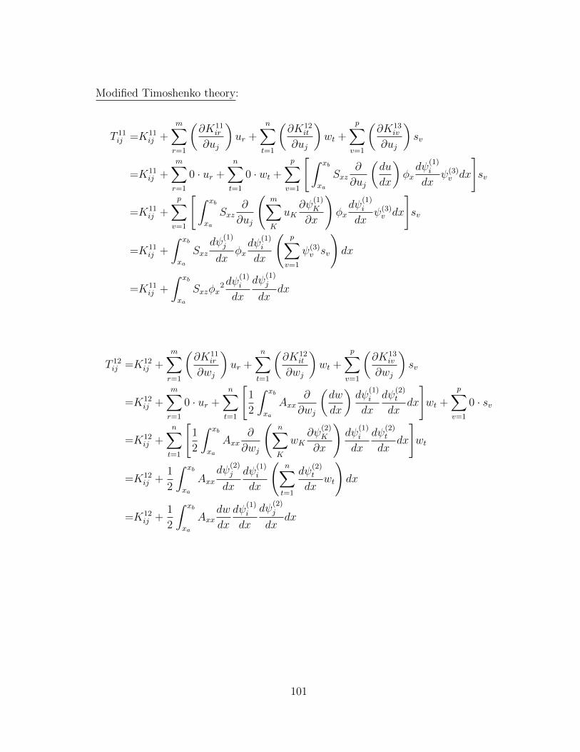
Modified Timoshenko theory:

T 11ij =K11

ij +m∑r=1

(∂K11

ir

∂uj

)ur +

n∑t=1

(∂K12

it

∂uj

)wt +

p∑v=1

(∂K13

iv

∂uj

)sv

=K11ij +

m∑r=1

0 · ur +n∑t=1

0 · wt +

p∑v=1

[∫ xb

xa

Sxz∂

∂uj

(du

dx

)φxdψ

(1)i

dxψ(3)v dx

]sv

=K11ij +

p∑v=1

[∫ xb

xa

Sxz∂

∂uj

(m∑K

uK∂ψ

(1)K

∂x

)φxdψ

(1)i

dxψ(3)v dx

]sv

=K11ij +

∫ xb

xa

Sxzdψ

(1)j

dxφxdψ

(1)i

dx

(p∑v=1

ψ(3)v sv

)dx

=K11ij +

∫ xb

xa

Sxzφx2dψ

(1)i

dx

dψ(1)j

dxdx

T 12ij =K12

ij +m∑r=1

(∂K11

ir

∂wj

)ur +

n∑t=1

(∂K12

it

∂wj

)wt +

p∑v=1

(∂K13

iv

∂wj

)sv

=K12ij +

m∑r=1

0 · ur +n∑t=1

[1

2

∫ xb

xa

Axx∂

∂wj

(dw

dx

)dψ

(1)i

dx

dψ(2)t

dxdx

]wt +

p∑v=1

0 · sv

=K12ij +

n∑t=1

[1

2

∫ xb

xa

Axx∂

∂wj

(n∑K

wK∂ψ

(2)K

∂x

)dψ

(1)i

dx

dψ(2)t

dxdx

]wt

=K12ij +

1

2

∫ xb

xa

Axxdψ

(2)j

dx

dψ(1)i

dx

(n∑t=1

dψ(2)t

dxwt

)dx

=K12ij +

1

2

∫ xb

xa

Axxdw

dx

dψ(1)i

dx

dψ(2)j

dxdx

101

T 13ij =K13

ij +m∑r=1

(∂K11

ir

∂sj

)ur +

n∑t=1

(∂K12

it

∂sj

)wt +

p∑v=1

(∂K13

iv

∂sj

)sv

=K13ij +

m∑r=1

[∫ xb

xa

Sxz∂

∂sj(φx)

2 dψ(1)i

dx

dψ(1)r

dxdx

]ur

+n∑t=1

[∫ xb

xa

Sxz∂

∂sj(φx)

dψ(1)i

dx

dψ(2)t

dxdx

]wt

+

p∑v=1

[∫ xb

xa

Sxzdu

dx

∂

∂sj(φx)

dψ(1)i

dxψ(3)v dx

]sv

=K13ij +

m∑r=1

[∫ xb

xa

Sxz∂

∂sj

(p∑K

sKψ(3)K

)2dψ

(1)i

dx

dψ(1)r

dxdx

]ur

+n∑t=1

[∫ xb

xa

Sxz∂

∂sj

(p∑K

sKψ(3)K

)dψ

(1)i

dx

dψ(2)t

dxdx

]wt

+

p∑v=1

[∫ xb

xa

Sxzdu

dx

∂

∂sj

(p∑K

sKψ(3)K

)dψ

(1)i

dxψ(3)v dx

]sv

=K13ij + 2

∫ xb

xa

Sxzφxψ(3)j

dψ(1)i

dx

(m∑r=1

dψ(1)r

dxur

)dx

+

∫ xb

xa

Sxzψ(3)j

dψ(1)i

dx

(n∑t=1

dψ(2)t

dxwt

)dx

+

∫ xb

xa

Sxzdu

dxψ

(3)j

dψ(1)i

dx

(p∑v=1

ψ(3)v sv

)dx

=K13ij + 3

∫ xb

xa

Sxzdu

dxφxdψ

(1)i

dxψ

(3)j dx+

∫ xb

xa

Sxzdw

dx

dψ(1)i

dxψ

(3)j dx

T 21ij = K21

ij +m∑r=1

(∂K21

ir

∂uj

)ur +

n∑t=1

(∂K22

it

∂uj

)wt +

p∑v=1

(∂K23

iv

∂uj

)sv

= K21ij +

m∑r=1

0 · ur +n∑t=1

0 · wt +

p∑v=1

0 · sv

= K21ij

102

T 22ij =K22

ij +m∑r=1

(∂K21

ir

∂wj

)ur +

n∑t=1

(∂K22

it

∂wj

)wt +

p∑v=1

(∂K23

iv

∂wj

)sv

=K22ij +

m∑r=1

[∫ xb

xa

Axx∂

∂wj

(dw

dx

)dψ

(2)j

dx

dψ(1)r

dxdx

]ur

+n∑t=1

[1

2

∫ xb

xa

Axx∂

∂wj

(dw

dx

)2dψ

(2)i

dx

dψ(2)t

dxdx

]wt +

p∑v=1

0 · sv

=K22ij +

m∑r=1

[∫ xb

xa

Axx∂

∂wj

(n∑K

wK∂ψ

(2)K

∂x

)dψ

(2)j

dx

dψ(1)r

dxdx

]ur

+n∑t=1

[1

2

∫ xb

xa

Axx∂

∂wj

(n∑K

wK∂ψ

(2)K

∂x

)2dψ

(2)i

dx

dψ(2)t

dxdx

]wt

=K22ij +

∫ xb

xa

Axxdψ

(2)j

dx

dψ(2)i

dx

(m∑r=1

dψ(1)r

dxur

)dx

+

∫ xb

xa

Axxdw

dx

dψ(2)j

dx

dψ(2)i

dx

(n∑t=1

dψ(2)t

dxwt

)dx

=K22ij +

∫ xb

xa

Axxdu

dx

dψ(2)i

dx

dψ(2)j

dxdx+

∫ xb

xa

Axx

(dw

dx

)2dψ

(2)i

dx

dψ(2)j

dxdx

T 23ij =K23

ij +m∑r=1

(∂K21

ir

∂sj

)ur +

n∑t=1

(∂K22

it

∂sj

)wt +

p∑v=1

(∂K23

iv

∂sj

)sv

=K23ij +

m∑r=1

[∫ xb

xa

Sxz∂

∂sj(φx)

dψ(2)i

dx

dψ(1)r

dxdx

]ur +

n∑t=1

0 · wt +

p∑v=1

0 · sv

=K23ij +

m∑r=1

[∫ xb

xa

Sxz∂

∂sj

(p∑K

sKψ(3)K

)dψ

(2)i

dx

dψ(1)r

dxdx

]ur

=K23ij +

∫ xb

xa

Sxzψ(3)j

dψ(2)i

dx

(m∑r=1

dψ(1)r

dxur

)dx

=K23ij +

∫ xb

xa

Sxzdu

dx

dψ(2)i

dxψ

(3)j dx

103

T 31ij =K31

ij +m∑r=1

(∂K31

ir

∂uj

)ur +

n∑t=1

(∂K32

it

∂uj

)wt +

p∑v=1

(∂K33

iv

∂uj

)sv

=K31ij +

m∑r=1

[∫ xb

xa

Sxz∂

∂uj

(du

dx

)φxψ

(3)i

dψ(1)r

dxdx

]ur +

n∑t=1

0 · wt

+

p∑v=1

[∫ xb

xa

Sxz∂

∂uj

(du

dx

)ψ

(3)i ψ(3)

v dx

]sv

=K31ij +

m∑r=1

[∫ xb

xa

Sxz∂

∂uj

(m∑K

uK∂ψ

(1)K

dx

)φxψ

(3)i

dψ(1)r

dxdx

]ur

+

p∑v=1

[∫ xb

xa

Sxz∂

∂uj

(m∑K

uK∂ψ

(1)K

dx

)ψ

(3)i ψ(3)

v dx

]sv

=K31ij +

∫ xb

xa

Sxzdψ

(1)j

dxφxψ

(3)i

(m∑r=1

dψ(1)r

dxur

)dx

+

∫ xb

xa

Sxzdψ

(1)j

dxψ

(3)i

(p∑v=1

ψ(3)v sv

)dx

=K31ij +

∫ xb

xa

Sxzdu

dxφxψ

(3)i

dψ(1)j

dxdx+

∫ xb

xa

Sxzφxψ(3)i

dψ(1)j

dxdx

T 32ij =K32

ij +m∑r=1

(∂K31

ir

∂wj

)ur +

n∑t=1

(∂K32

it

∂wj

)wt +

p∑v=1

(∂K33

iv

∂wj

)sv

=K32ij +

m∑r=1

[∫ xb

xa

Sxz∂

∂wj

(dw

dx

)ψ

(3)i

dψ(1)r

dxdx

]ur +

n∑t=1

0 · wt +

p∑v=1

0 · sv

=K32ij +

m∑r=1

[∫ xb

xa

Sxz∂

∂wj

(n∑K

wK∂ψ

(2)K

∂x

)ψ

(3)i

dψ(1)r

dxdx

]ur

=K32ij +

∫ xb

xa

Sxzdψ

(2)j

dxψ

(3)i

(m∑r=1

dψ(1)r

dxur

)dx

=K32ij +

∫ xb

xa

Sxzdu

dxψ

(3)i

dψ(2)j

dxdx

104

T 33ij =K33

ij +m∑r=1

(∂K31

ir

∂sj

)ur +

n∑t=1

(∂K32

it

∂sj

)wt +

p∑v=1

(∂K33

iv

∂sj

)sv

=K33ij +

m∑r=1

[∫ xb

xa

Sxz∂

∂sj

(φx +

du

dxφx

)ψ

(3)i

dψ(3)r

dxdx

]ur +

n∑t=1

0 · wt

+

p∑v=1

[∫ xb

xa

1

2Axx

∂

∂sj(φx)

2 ψ(3)i ψ(3)

v + Sxz∂

∂sj

(φxdφxdx

)dψ

(3)i

dxψ(3)v

+ Sxz∂

∂sj

(φxdφxdx

)ψ

(3)i

dψ(3)v

dx

dx

]sv

=K33ij +

m∑r=1

[∫ xb

xa

Sxz

[∂

∂sj

(p∑K

sKψ(3)K

)+du

dx

∂

∂sj

(p∑K

sKψ(3)K

)]

× ψ(3)i

dψ(1)r

dxdx

]ur

+

p∑v=1

[∫ xb

xa

1

2Axx

∂

∂sj

(p∑K

sKψ(3)K

)2

ψ(3)i ψ(3)

v

+ Sxz

[∂

∂sj

(p∑K

sKψ(3)K

)dφxdx

+ φx∂

∂sj

(p∑K

sK∂ψ

(3)K

∂x

)]dψ

(3)i

dxψ(3)v

+ Sxz

[∂

∂sj

(p∑K

sKψ(3)K

)dφxdx

+ φx∂

∂sj

(p∑K

sK∂ψ

(3)K

∂x

)]ψ

(3)i

dψ(3)v

dx

dx

]sv

=K33ij +

∫ xb

xa

Sxz

(ψ

(3)j +

du

dxψ

(3)j

)ψ

(3)i

(m∑r=1

dψ(1)r

dxur

)dx

+

∫ xb

xa

Axxφxψ

(3)j ψ

(3)i

(p∑v=1

ψ(3)v sv

)

+ Sxz

(ψ

(3)j

dφxdx

+ φxdψ

(3)j

dx

)dψ

(3)i

dx

(p∑v=1

ψ(3)v sv

)

+ Sxz

(ψ

(3)j

dφxdx

+ φxdψ

(3)j

dx

)ψ

(3)i

(p∑v=1

dψ(3)v

dxsv

)dx

105

=K33ij +

∫ xb

xa

Sxzdu

dx

(ψ

(3)i ψ

(3)j +

du

dxψ

(3)i ψ

(3)j

)dx

+

∫ xb

xa

Axxφx

2ψ(3)i ψ

(3)j + Sxzφx

(dφxdx

dψ(3)i

dxψ

(3)j + φx

dψ(3)i

dx

dψ(3)j

dx

)

+ Sxzdφxdx

(dφxdx

ψ(3)i ψ

(3)j + φxψ

(3)i

dψ(3)j

dx

)dx

106

bending, vibration and buckling response...

Documents