benchmarking state-of-the-art classification algorithms for credit scoring… · 1 benchmarking...
TRANSCRIPT

1
Benchmarking state-of-the-art classification algorithms for credit scoring: A ten-year update
Stefan Lessmanna,*, Hsin-Vonn Seowb, Bart Baesenscd, Lyn C. Thomasd a Institute of Information Systems, University of Hamburg
b Nottingham University Business School, University of Nottingham-Malaysia Campus c Department of Decision Sciences & Information Management, Catholic University of Leuven
dSchool of Management, University of Southampton, Highfield, Southampton, SO17 1BJ, United Kingdom
Abstract
Ten years have passed since Baesens et al. published their benchmarking study of
classification algorithms in credit scoring [Baesens, B., Van Gestel, T., Viaene, S., Stepanova,
M., Suykens, J., & Vanthienen, J. (2003). Benchmarking state-of-the-art classification algorithms
for credit scoring. Journal of the Operational Research Society, 54(6), 627-635.]. The interest in
predictive methods for scorecard construction is unbroken, and the work of Baesens et al. is still
held in high regard. However, there have been numerous advancements in predictive modeling,
including novel learning methods and techniques to reliably assess the performance of alternative
scorecards. Neither Baesens et al. nor other studies in the retail credit scoring literature reflect
these developments. The objective of this paper is to close this research gap. To that end, we
update the study of Baesens et al. and compare several novel classification algorithms to the
state-of-the-art in credit scoring. In addition, we repeat our benchmark for several performance
measures and examine the degree to which these differ in their assessment of candidate
scorecards. Our study provides valuable insight for professionals and academics in credit scoring.
The paper helps practitioners to stay abreast of technical advancements in predictive modeling.
From an academic standpoint, the study provides an independent assessment of recent scoring
methods and offers a new baseline to which future approaches can be compared.
* Corresponding author: Tel.: +49-40-42838-4706, Fax: +49-40-42838-5535. a Institute of Information Systems, University of Hamburg, Von-Melle-Park 5, 20146 Hamburg, Germany;
[email protected] b Nottingham University Business School, University of Nottingham-Malaysia Campus, Jalan Broga,
43500Semenyih, Selangor Darul Ehsan, Malaysia; [email protected] c Department of Decision Sciences & Information Management, Catholic University of Leuven, Naamsestraat 69, B-
3000 Leuven, Belgium; [email protected] d School of Management, University of Southampton, Highfield, Southampton, SO17 1BJ, United Kingdom;

2
1 Introduction
Credit Scoring is concerned with assessing financial risks and informing managerial decision
making in the money lending business. Generally speaking, a credit score is a model-based
estimate of the probability that a borrower will show some undesirable behavior in the future. A
classic example is application scoring. To decide on an application for some credit product, the
bank employs a predictive model, called a scorecard, to estimate how likely the applicant is to
default (e.g., Crook et al., 2007). Typically, the term credit scoring refers to credit decisions in
the retail business. The management of corporate or national credit is considered in the literature
on business failure prediction or credit rating analysis, respectively (e.g., Kumar & Ravi, 2007;
Zhang et al., 2010b).
The retail business is of considerable importance. For example, the total volume of consumer
loans hold by commercial banks in the US in May 2013 was $1,132.4 bn; compared to
$1,540.6 bn in the corporate business.1 In the UK, loans and mortgages to individuals were even
higher than corporate loans in 2012 (£11,676 m c.f. £10,388 m).2 Credit scoring is also employed
to approve new credit cards. On a global scale, the total number of (general purpose) credit cards
circulating in 2011 was 2,039.3 m, and these were used in 64,24 bn transactions (Nielsen, 2012).
Especially emerging countries have seen impressive growth figures in the number of credit cards
in the recent past (Akkoc, 2012). Given these figures, it is clear that financial institutions
critically depend on quantitative decision aids to enable accurate risk assessments in consumer
lending (e.g., Thomas, 2010). This is the scope of credit scoring, which Crook et al. (2007, p.
1448) consider as “one of the most successful applications of statistics and OR in industry”.
This paper concentrates on empirical prediction models that estimate the entry probability of
discrete events and default events in particular. Such PD models (probability of default) are well
established in the literature (e.g., Hand & Henley, 1997; Thomas, 2000). Classification analysis is
arguably the prevailing approach to develop PD scorecards, and many studies have explored the
effectiveness of different classification algorithms in credit scoring (e.g., Finlay, 2011; Paleologo
et al., 2010; West et al., 2005). In such a setting, it is common to assess the effectiveness of an
algorithm in terms of the predictive accuracy of the resulting scorecard.
1 Data from the Federal Reserve Board, H8, Assets and Liabilities of Commercial Banks in the United States
(http://www.federalreserve.gov/releases/h8/current/). 2 Data from ONS Online, SDQ7: Assets, Liabilities and Transactions in Finance Leasing, Factoring and Credit
Granting: 1st quarter 2012 (http://www.ons.gov.uk).

3
A seminal study in the field is the benchmarking experiment of Baesens et al. (2003b), who
contrast 17 state-of-the-art classifiers on eight real-world credit scoring data sets. Given its date
of publication, it is clear that this study misses several of the latest advancements in predictive
learning, including novel classification algorithms, better indicators of predictive accuracy, and
statistical tests to reliably compare different algorithms (e.g., García et al., 2010; Hand &
Anagnostopoulos, 2013; Huang et al., 2011). Therefore, the objective of this paper is to update
and extend the benchmarking experiment of Baesens et al. (2003b).
Studies subsequent to Baesens et al. (2003b) have addressed some of the shortcomings
mentioned above. The question whether novel classifiers produce better scorecards than
established techniques has received particular attention and let to the evaluation of, amongst
others, ensemble methods (Paleologo et al., 2010), neuro-fuzzy inference systems (Akkoc, 2012),
and multiple classifier architectures (Finlay, 2011), all of which were not considered in Baesens
et al. (2003b). Given ample research in the field, it is important to clarify how this study
contributes to the literature. To that end, we briefly summarize the findings from a detailed
analysis of the PD modeling literature (see Section 2.2), in which we identity several remaining
research gaps.
First, most studies that follow Baesens et al. (2003b) are of limited scope and consider only a
few classifiers and/or credit scoring data sets. This raises issues related with external validity.
Employing multiple different data sets (e.g., data from different companies) is useful to examine
the robustness of a scorecard with respect to different environmental conditions. In a similar
fashion, examining several different – established and novel – classifiers is important to obtain a
clear view of the state-of-the-art, and how it advances over time.
Second, many studies propose a novel modeling methodology and compare it to some
reference classifier(s). This may introduce bias, for example because the developers of the new
technique are naturally more adept with their method than an external user would be, and/or
because the new method may have been tuned more elaborately than reference methods (Hand,
2006; Thomas, 2010). A benchmarking experiment, on the other hand, compares many
alternative classifiers without prior hypotheses which method performs best.
Third, empirical practices to compare scorecards do not reflect the latest advancements in
predictive learning. On the one hand, this critic applies to the area under a receiver operating
characteristics curve (AUC), which is a common scorecard assessment criterion. However, when
comparing scorecards in terms of the AUC, one implicitly assumes that the cost distributions

4
associated with classification errors differ across scorecards (Hand & Anagnostopoulos, 2013).
This assumption is implausible, especially in a credit scoring benchmark. It is thus useful to
revisit previous results in the light of improved performance indicators such as the H-measure
(Hand, 2009). Similarly, elaborate frameworks for statistical hypothesis testing in classifier
comparisons have been proposed (García et al., 2010). However, neither Baesens et al. (2003b)
nor a subsequent study has used such techniques to interpret benchmarking results.
Finally, there are several recently developed classification algorithms that, despite
encouraging results in other areas, have not considered in credit scoring and/or have not been
systematically compared to each other. Examples include extreme learning machines (Huang et
al., 2011), rotation forests (Rodriguez et al., 2006), or the whole family of selective ensemble
methods (e.g., Tsoumakas et al., 2009).
The objective of this paper is close the research gaps identified above. Put differently, we
strive to provide a holistic view of the state-of-the-art in predictive modeling and how it can
support managerial decision making in the credit industry. In pursuing this objective, we make
the following contributions: First, using the data of Baesens’s et al. (2003) original study and two
novel data sets of considerable size, we conduct a large-scale benchmark of 41 classification
methods on seven real-world credit-scoring data sets. Several of these methods are new to the
community and for the first time assessed in a credit scoring context. Second, we examine the
correspondence between empirical results obtained using traditional versus novel performance
indicators. In particular, we clarify the reliability of scorecard comparisons in the light of new
findings related with the conceptual shortcomings of the AUC (Hand, 2009; Hand &
Anagnostopoulos, 2013). Finally, we illustrate the use of advanced nonparametric testing
procedures to secure empirical findings and, thereby, offer useful guidance for future studies.
The remainder of the paper is organized as follows: In Section 2, we review related literature
and analyze the empirical practices in previous classifier comparisons. Afterwards, we
summarize the classification algorithms which we compare (Section 3) and describe the setup of
our benchmarking experiment (Section 4). We report and discuss our empirical results in
Section 5. Section 6 concludes the paper.

5
2 Literature review
The literature review consists of two parts. First, we review related work associated with
predictive modeling in the credit industry to put this study. Next, we examine previous studies in
retail credit scoring to elaborate the specific research gaps that this study addresses.
2.1 Related work
A large body of literature explores the development, application, and evaluation of predictive
decision support models in the credit industry. We distinguish different research streams along
two dimensions, the subject of the risk assessment and the lifecycle of a credit scorecard.
Relevant scoring subjects include nations, municipalities, bond offerings, enterprises of
different sizes, and retail customers. Credit rating analysis concentrates on the former subjects
and assesses their capability and willingness to meet payable obligations. A common application
of predictive modeling is to mimic the evaluation process of rating agencies such as Moody’s
(e.g., Hájek, 2011), and, more specifically, to estimate the transition probability of an entity with
given rating being moved to a higher/lower risk category (e.g., Kim & Sohn, 2008; Zhang et al.,
2010b). Corporate risk models are also developed by financial institutions to inform lending
decisions and to predict bankruptcy in particular (e.g, Fethi & Pasiouras, 2010; Kumar & Ravi,
2007). A sub-stream within the corporate risk modeling literature considers the peculiarities of
small-and-medium enterprises (e.g., Kim & Sohn, 2010; Sohn & Kim, 2007) or micro-
entrepreneurs (e.g., Bravo et al., 2013), for example to support (governmental) funding decisions.
An important difference between corporate and consumer risk models concerns the
explanatory variables that underline the development of a credit score (e.g., Thomas, 2010). The
former employ data from balance sheets and other financial ratios or macro-economic indicators
(e.g., Psillaki et al., 2009; Takada & Sumita, 2011; Van Gestel et al., 2006), whereas retail
scoring models use data from application forms, customer demographics, and possibly
transactional data from the customer history (e.g., Crook et al., 2007; Hand & Henley, 1997;
Thomas et al., 2005). The differences between these types of variables suggest that specific
modeling challenges arise in corporate versus consumer credit scoring. Therefore, many studies –
including this one – concentrate on either the corporate or the retail business.
The lifecycle of a scorecard includes different stages, from gathering and preparing relevant
data, over estimating a credit score using a formal induction algorithm, to the deployment,
monitoring and recalibration of the scorecard. All stages have been explored in the literature. For

6
example, relevant questions during data gathering and preparation concern the handling of
missing values (e.g., Florez-Lopez, 2010), the selection of a predictive set of explanatory
variables (e.g., Falangis & Glen, 2010; Liu & Schumann, 2005), and how biases due to an
underrepresentation of bad risks in scoring data sets (e.g., Brown & Mues, 2012; Marqués et al.,
2013; Paleologo et al., 2010) or the more fundamental problem that repayment behavior is, by
definition, only observable for previously accepted (i.e., seemingly good) customers, can be
overcome (e.g., Banasik & Crook, 2007; Banasik et al., 2003; Wu & Hand, 2007).
Once a prepared data set is available, a variety of prediction methods facilitate estimating
different aspects of credit risk. In particular, the Basel II Capital Accord requires financial
institutions, who adopt an internal rating approach, to develop three types of risk models to
estimate, respectively, the probability of default (PD), the exposure at default (EAD), and the loss
given default (LGD).
The development of EAD and LGD prediction models has become a popular topic in recent
research (e.g., Bellotti & Crook, 2012; Loterman et al., 2012; Somers & Whittaker, 2007).
However, the majority of credit scoring studies concentrate on PD modeling using either
classification or survival analysis. Survival analysis models predict default probabilities for
different time periods. This is useful to estimate when a customer will default (e.g., Bellotti &
Crook, 2009b; Stepanova & Thomas, 2002; Tong et al., 2012). Classification analysis, on the
other hand, benefits from an unmatched variety of modeling methods and represents the
prevailing modeling approach in the literature.
Finally, it is important to continuously monitor scorecard performance after deployment to
explore its robustness toward changes in customer behavior and to recalibrate the scorecard when
its performance degrades (e.g., Pavlidis et al., 2012; Sohn & Ju; Thomas et al., 2001). An
interesting direction in the literature on adaptive scoring addresses the problem that some lenders,
and fraudsters in particular, act strategic to circumvent formal risk assessment procedures (e.g.,
Boylu et al., 2010).
2.2 Classification analysis in retail credit scoring
We concentrate on retail credit scoring, and, more specifically, on classification-based risk
modeling for individual customers. This approach is well represented in the literature. We review
previous studies in Table 1. In particular, we concentrate on the experimental practices in credit
scoring studies published in 2003 and thereafter. This is to confirm the need for an update of

7
Baesens et al. (2003b) and to identify gaps in research. Another goal is to clarify the degree to
which different types of ensemble classifiers, which were not considered in Baesens et al.
(2003b), have been covered in subsequent work. To that end, we study three dimensions related
with empirical classifier comparisons: the type of credit scoring data, the employed classification
algorithms, and the indicators to assess these algorithms.
TABLE 1: ANALYSIS OF CLASSIFIER COMPARISONS IN RETAIL CREDIT SCORING
Retail credit scoring study (in chronological order)
Data* Classifiers** Evaluation***
No. of data
sets
Observations / variables per data set
No. of
classifiers
AN
N
SV
M
EN
S
S-E
NS
TM
AU
C
SH
T
(Baesens et al., 2003b) 8 4,875 21 17 X X X X P
(Malhotra & Malhotra, 2003) 1 1,078 6 2 X X P
(Atish & Jerrold, 2004) 2 610 16 5 X X X P
(He et al., 2004) 1 5,000 65 4 X X
(Lee & Chen, 2005) 1 510 18 5 X X
(Hand et al., 2005) 1 1,000 20 4 X X
(Ong et al., 2005) 2 845 17 6 X X
(West et al., 2005) 2 845 19 4 X X X P
(Huang et al., 2006b) 1 10,000 n.a. 10 X X
(Lee et al., 2006) 1 8,000 9 5 X X
(Li et al., 2006) 1 600 17 2 X X X P
(Xiao et al., 2006) 3 972 17 13 X X X X P
(Huang et al., 2007) 2 845 19 4 X X F
(Yang, 2007) 2 16,817 85 3 X X
(Abdou et al., 2008) 1 581 20 6 X X A
(Sinha & Zhao, 2008) 1 220 13 7 X X X X A
(Tsai & Wu, 2008) 3 793 16 3 X X X P
(Xu et al., 2008) 1 690 15 4 X X
(Yu et al., 2008) 1 653 13 7 X X X
(Abdou, 2009) 1 1,262 25 3 X
(Bellotti & Crook, 2009a) 1 25,000 34 4 X X
(Chen et al., 2009) 1 2,000 15 5 X X
(Šušteršič et al., 2009) 1 581 84 2 X X
(Tsai et al., 2009) 1 1,877 14 4 X X
(Yu et al., 2009a) 3 959 16 10 X X XY X X P
(Yu et al., 2009b) 1 1,225 14 8 X X X X P
(Zhang et al., 2009) 1 1,000 102 4 X
(Hsieh & Hung, 2010) 1 1,000 20 4 X X Y X

8
(Martens et al., 2010) 1 1,000 20 4 X X
(Twala, 2010) 2 845 18 5 X X
(Zhang et al., 2010a) 2 845 17 11 X X X X
(Zhou et al., 2010) 2 1,113 17 25 X X X X X
(Li et al., 2011) 2 845 17 11 X X
(Finlay, 2011) 2 104,649 47 18 X XY X P
(Ping & Yongheng, 2011) 2 845 17 4 X X X
(Wang et al., 2011) 3 643 17 13 X X XY X
(Yap et al., 2011) 1 2,765 4 3 X
(Yu et al., 2011) 2 845 17 23 X X X
(Akkoc, 2012) 1 2,000 11 4 X X X
(Brown & Mues, 2012) 5 2,582 30 9 X X X X F/P
(Hens & Tiwari, 2012) 2 845 19 4 X X
(Li et al., 2012) 2 672 15 5 X X X
(Marqués et al., 2012a) 4 836 20 35 X X X X F/P
(Marqués et al., 2012b) 4 836 20 17 X X XY X X F/P
(Kruppa et al., 2013) 1 65,524 17 5 X X
Counts 45 30 24 18 3 40 10 17
Percent 100 67 53 40 7 89 22 38
Mean 1.9 6,167 24 7.8
Median 1.0 959 17 5.0
* We report the mean value of observations and independent variables for studies that employ multiple data sets. Eight studies mix retail and corporate credit data. Table 1 shows the retail data sets only.
** Abbreviations have the following meaning: ANN=Artificial neural network, SVM=Support vector machine, ENS=Ensemble classifier, S-ENS=Selective Ensemble. An X indicates that a study includes a classifier. In the ENS column, entries of X and Y indicate that a study includes homogeneous and heterogeneous ensembles, respectively.
*** Abbreviations have the following meaning: TM=Threshold metric (e.g., classification error, error costs, true positive rate, etc.), AUC=Area under receiver operating characteristics curve, SHT=Statistical hypothesis testing. In the last columns, we use codes to report the type of statistical test used for classifier comparisons. Codes have the following meaning: P=Pairwise comparison (e.g., paired t-test), A=Analysis of variance, F=Friedman test, F/P=Friedman test together with post-hoc test (e.g., Demšar, 2006).
Several conclusions emerge from Table 1. First, it is common practice to compare classifiers
on only a few data sets (1.9 on average). Moreover, the data sets are typically of small size and
contain only a few independent variables. This does not represent the credit scoring data sets that
occur in industry and might introduce bias (e.g., Finlay, 2011; Hand, 2006). Another issue, not
explicitly visible Table 1, is that the majority of studies rely on the two credit scoring data sets
Australian and Germen Credit, which are available in the UCI Machine Learning Library
(Asuncion & Newman, 2010). This may also introduce bias if new algorithms are explicitly
designed to achieve high accuracy on these two data sets.

9
Second, the number of classification algorithms varies considerably across credit scoring
studies (e.g., from 2 to 35). Although some studies employ a larger number of different
algorithms, it is rare that multiple state-of-the-art methods are systematically compared to each
other. For example, a larger number of classifiers can be the result of factorial designs that pair
some classification algorithms with some homogeneous ensemble algorithms (e.g., Marqués et
al., 2012a; Wang et al., 2011). This is useful to answer specific research questions (e.g., which
base classifiers works best in a bagging framework), but does not address the more general
question whether certain modeling approaches are particularly well suited for credit scoring, and
to what extent recent developments in predictive learning offer sizeable advantages over more
established scoring techniques.
Third, ensemble classifiers have been covered in the credit scoring literature. The focus is
typically on homogeneous ensembles. Heterogeneous ensembles are rarely considered. However,
a comprehensive comparison of thirteen different approaches has recently been conducted
(Finlay, 2011), so that this family of ensembles is reasonably well represented in the literature.
This is not the case for selective ensemble classifiers. Just two studies include such techniques,
and they both employ one selective ensemble only. Consequently, a systematic comparison of
different selective ensemble classifiers is missing in credit scoring literature. This might be an
important research gap because selective ensemble methods have shown very promising results
in other areas (e.g., Partalas et al., 2010; Woloszynski et al., 2012) and secured winning entries in
prestigious data mining competitions such as the KDD Cup 2009 (Niculescu-Mizil et al., 2009).
Fourth, many classifier comparisons rely on a single evaluation measure or measures of the
same type. In general, evaluation criteria measures split into three types of measures. Those that
measure the discriminatory ability of the scorecard (AUC, H-measure); those that measure the
accuracy of the scorecards’ probability predictions (Brier Score) and those that measure the
correctness of the scorecards’ categorical predictions (classification error, recall, misclassification
costs, etc.). Different types of indicators embody a different notion of classifier performance
(e.g., Caruana & Niculescu-Mizil, 2006). However, few studies include multiple evaluation
measures of different types. For example, none of the reviewed studies uses performance
measures such as the Brier Score, which assess the accuracy of probabilistic predictions. This
misses an important aspect of scorecard performance. To inform risk management decisions,
financial institutions require default probability estimates that are not only accurate but also well
calibrated (e.g., Blochlinger & Leippold, 2011). Moreover, it is noteworthy that previous studies

10
have not considered the H-measure to assess classifier performance. The H-measure exhibits
several features that make it ideal for comparing different classifiers and overcomes potentially
severe limitations of the AUC (Hand, 2009).
Last, several previous studies fall short of securing conclusions by means of formal statistical
testing procedures. Furthermore, the majority of studies that use statistical tests adopt less
suitable approaches. For example, the assumptions of parametric tests such as analysis of
variance or the t-test, which are used in some studies, are typically violated in classifier
comparisons (e.g., Demšar, 2006). More importantly, many studies perform multiple pairwise
comparisons of classifiers (shown by a ‘P’ in the last column of Table 1) using some level of
significance (e.g., 0.05). Without appropriate adjustment, this approach leads to an elevation
of the family-wise error beyond the stated level of , and thus introduces bias (e.g., García et al.,
2010). Demšar (2006) recommends the combination of a Friedman test with post-hoc test for
classifier benchmarks. Only three studies follow this approach (i.e., ‘F/P’ in Table 1). However, a
possible issue with these studies is that they use post-hoc tests with relative low power (e.g.,
García et al., 2010).
The above observations support our view that an update of the study of Baesens et al. (2003b)
is important. In doing so, we overcome several of the issues in previous studies through i)
conducting a large-scale comparisons of several established and novel classification algorithms
including selective ensemble methods, ii) using multiple data sets of considerable size, iii) several
conceptually different performance criteria, and iv) suitable statistical testing procedures.
3 Classification algorithms for scorecard construction A scorecard is an instrument that supports decision making in the credit industry. Let
, , … , ∈ be an m-dimensional vector that characterizes an application for
some credit product such as a loan. The performance of previously approved loans is known to
the decision maker. Let ∈ 1, 1 be a binary response variable that indicates whether a
default event was observed for the ith loan. In the following, we assume that values of -1 and +1
represent performing and non-performing loans, respectively. When deciding on an application
with characteristics , it is important to have an estimate of the posterior probability 1|
that the loan will turn out to be non-performing, if it is granted. A credit scorecard provides such

11
an estimate. A decision maker can then compare the model-estimated 1| to a threshold, ;
approving the loan if 1| , and rejecting it otherwise.
The problem of estimating 1| belongs to the field of classification analysis (e.g., Hand,
1997). Specifically, a scorecard is the result of applying a classification algorithm to a data set
, of past loans. Several alternative algorithms have been proposed in the literature
(e.g., Hastie et al., 2009). We distinguish three types of algorithms: individual classifiers,
homogenous ensemble classifiers, and heterogeneous ensemble classifiers. The first group
includes methods such as logistic regression or artificial neural networks, where the eventual
scorecard consists of a single classification model. The latter two combine the predictions of
multiple classification models, called base models. Homogeneous ensembles create base models
using one classification algorithm, whereas heterogeneous ensembles use different algorithms.
To get a clear view on the relative effectiveness of different classification algorithms for retail
credit risk assessment, we compare a large set of 16 individual classifiers, 8 homogenous
ensembles, and 17 heterogeneous ensembles. Most classifiers offer some meta-parameters to tune
the algorithm to a particular task. Examples include the number of hidden nodes in a neural
network or the kernel function in a support vector machine (e.g., Baesens et al., 2003b). Relying
on literature recommendations and our own experience, we define several candidate settings for
such meta-parameters and create one classification model per setting. That is, we produce
multiple models with a single classification algorithm. Our motivation for this approach is
twofold. First, a careful exploration of the meta-parameter space ensures that we obtain a good
estimate how well a classifier can perform in a given task (i.e., on a given data set). This is
important when comparing alternative classifiers to each other. Second, using different meta-
parameter settings allows us to develop a large number of (base) models for heterogeneous
ensemble classifiers (e.g., Caruana et al., 2006).
Table 2 reports the algorithms as well as the number of classification models per algorithm.
An extended version of this table including the specific meta-parameter settings and
implementation details is available in Appendix I. Given the scope of the comparison, a fully-
comprehensive discussion of all algorithms is beyond the scope of the paper (see, e.g., Hastie et
al., 2009 for a detailed discussion; Kuncheva, 2004). However, to keep the paper self-contained
and to illustrate the philosophies underneath different algorithms, the following chapters provide
an overview of the classifiers considered here. In addition, Figure 1 gives a graphical illustration

12
of the modeling process to create scorecards using individual, homogeneous ensemble, and
heterogeneous ensemble classifiers.
Figure 1: Classifier development and evaluation process
TABLE 2: CLASSIFICATION ALGORITHMS CONSIDERED IN THE BENCHMARKING STUDY
Base model selection
Classification algorithm Acronym Number of
models1
Ind
ivid
ual
cla
ssif
ier
n.a.
Bayesian Network B-Net 4
CART CART 10
Extreme learning machine ELM 120
Kernalized ELM ELM-K 200
k-nearest neighbor kNN 22
J4.8 J4.8 36
Linear discriminant analysis2 LDA 1
Linear support vector machine SVM-L 29
Logistic regression2 LR 1
Multilayer perceptron artificial neural network ANN 171

13
Naive Bayes NB 1
Quadratic discriminant analysis2 QDA 1
Radial basis function neural network RbfNN 5
Regularized logistic regression LR-R 27
SVM with radial basis kernel function SVM- Rbf 300
Voted perceptron VP 5
Classification models from individual classifiers 16 933
Hom
ogen
ous
ense
mb
les
n.a.
Alternating decision tree ADT 5
Bagged decision trees Bag 9
Bagged MLP BagNN 4
Boosted decision trees Boost 48
Logistic model tree LMT 1
Random forest RF 30
Rotation forest RotFor 25
Stochastic gradient boosting SGB 9
Classification models from homogeneous ensembles 8 131
Het
erog
eneo
us e
nse
mb
les
n.a. Simple average ensemble AvgS 1
Weighted average ensemble AvgW 1
Static direct
Complementary measure CompM 4
Ensemble pruning via reinforcement learning EPVRL 4
GASEN GASEN 4
Hill-climbing ensemble selection HCES 12
HCES with bootstrap sampling HCES-Bag 16
Matchting pursuit optimization of ensemble classifiers MPOCE 1
Stacking Stack 6
Top-T ensemble Top-T 12
Static indirect
Clustering using compound error CuCE 1
k-Means clustering k-Means 1
Kappa pruning KaPru 4
Margin distance minimization MDM 4
Uncertainty weighted accuracy UWA 4
Dynamic Probabilistic model for classifier competence PMCC 1
k-nearest oracle kNORA 1
Classification models from heterogeneous ensembles 17 77
Overall number of classification algorithms and models 41 1141 1 The number of models per classification algorithm results from using multiple settings for meta-parameters. The
specific values are available in Table 11 in Appendix I. 2 To overcome problems associated with multicollinearity in high-dimensional data sets, we use correlation-based
feature selection (Hall, 2000) to reduce the variable set prior to building a classification model.

14
3.1 Individual classifiers
The individual classifiers used in this study represent a diverse set of different approaches.
The most popular approach in credit scoring is logistic regression (LR). LR strives to estimate
1| using a logit-link function to model the relationship between independent variables
(IVs) and the response variable:
1|1
1 exp ∑.
(1)
Given a sample , , LR determines the model parameters and through
minimizing the negative log-likelihood function:
min,ℓ ln 1 ln , (2)
where we use as a shorthand form of 1| . Note that (2) assumes that examples
of the positive and the negative class are coded 1 and 0, respectively.
Maximum likelihood methods may become unstable if the number of IVs is large and/or if
these are heavily correlated (e.g.,Vapnik & Kotz, 2006). Therefore, regularized logistic
regression (LR-R) adds a complexity penalty to (2). As a consequence, LR-R balances the
conflicting goals of high fit and low complexity when estimating model parameters. In this work,
we use an L2 (ridge) penalty, which results in the following objective to devise a LR-R scorecard
(e.g., Chih-Jen et al., 2008; Fan et al., 2008):
min,
‖ , ‖ ℓ. (3)
The meta-parameter allows the user to control the trade-off between low complexity and
high fit. The linear support vector machine (SVM-L) considers a similar objective but uses a
different loss-function to measure model fit. In particular, it employs hinge-loss and solves the
following objective using dual coordinate descend methods (e.g., Chih-Jen et al., 2008; Fan et al.,
2008).
min,
‖ , ‖ max 1 ⋅ , 0 . (4)
The voted perceptron classifier (VP) can be considered a simplified SVM-L, which uses an
online algorithm to solve (4) without the ridge penalty (Freund & Schapire, 1999).
The radial basis function SVM (SVM- Rbf) is a nonlinear version of SVM-L. This means
that it can account for nonlinear relationships between IVs and the response variable, which

15
neither of the above classifiers can accommodate (e.g., Baesens et al., 2003b). To capture
nonlinear patterns, SVM- Rbf maps the input data to a higher-dimensional space. It then
constructs a linear classifier in the transformed space, which is equivalent to a nonlinear
classification in the original input space.
Artificial neural networks (ANN) are another class of nonlinear classifiers. The study
incorporates four different types of feed-forward neural networks. In general, a feed-forward
neural network consists of an input layer, a hidden, and an output layer. Each layer consists of
multiple information processing units called neurons. The neurons of one layer are fully-
connected to the neurons of the next layer, whereby the IVs represent the input layer neurons.
The number of neurons in the output layer is also fixed and set to one in our study. This is a
common setup to estimate posterior probabilities (e.g., Hastie et al., 2009). Finally, the number of
neurons in the hidden layer, Z, is a meta-parameter. Let be a vector of weights that connect the
input neurons to the zth hidden neuron, a threshold attached to hidden neuron z, and let be
some nonlinear function. We can then write the output of the hidden layer as follows:
, , ⋮ . (5)
In a similar way, the result of the network, , is:
, , , , (6)
where denotes the weight vector connecting the hidden and the output layer, and some
function that transform the result of the output neuron.
Multilayer perceptron artificial neural networks (ANN) employ sigmoidal functions for
and , and determine the model parameters ( , , and ) through minimizing some loss-
function using gradient-based methods. Specifically, we consider ANN with logistic activation
functions in the hidden and output layer. To create an ANN classifier, we solve (7) using a quasi-
Newton algorithm (Nabney, 2002), where is once more a regularization parameter to penalize
model complexity and prevent overfitting.
min , ‖ ‖ . (7)

16
The radial basis function network (RbfNN) is a second, closely related network classifier. It
uses a normalized Gaussian radial basis function in the hidden layer to compute the distance of an
example to pre-defined reference points, which we determine through k-means clustering (Witten
& Eibe, 2011). The number of cluster is a meta-parameter of RbfNN. Finally, extreme learning
machines (ELMs) are a recently introduced variant of neural networks that possess some
advantages compared to RbfNN and ANN (e.g., Huang et al., 2006a). ELMs are grounded in a
mathematical proof that a single-hidden layer feed-forward network with randomly generated
hidden-layer-weights is a universal approximator if the weights connecting the hidden and the
output layer, , are appropriately chosen (Guang-Bin et al., 2006). This result facilitates building
ELM classifiers without using resource-intensive training algorithms such as gradient descend.
Instead, it is sufficient to solve ⋅ , where , … , are the training data class labels
and is the hidden layer output matrix (e.g., Huang et al., 2006a):
, , ⋯ , ,⋮ ⋯ ⋮, , ⋯ , ,
(8)
The original ELM offers two meta-parameters, the number of neurons in the hidden layer and
their activation function. Furthermore, a version of the ELM that supports kernel functions
(ELM-K) has recently been proposed (Huang et al., 2012). This classifier features additional
meta-parameters (e.g., the width of the Rbf or the degree of a polynomial kernel function).
The previous algorithms take a direct approach to solve the classification problem. They
estimate either 1| or create a discriminant function that separates examples from
adjacent classes. A different approach is to estimate class-conditional probabilities and to covert
these into posterior probabilities using Bayes rule. Let | denote the class-conditional
probability that an example from class 1 exhibits characteristics , and 1 the
prior probability of class +1. According to Bayes rule:
1|| 1 ⋅ 1
. (9)
Note that the probability of observing an example with characteristics , , does not depend
on class memberships and is thus irrelevant for classification.
Linear discriminant analysis (LDA) approximates | 1 by means of a multivariate
normal distribution assuming identical covariance matrixes for both classes. Quadratic
discriminant analysis (QDA) relaxes the identical covariance assumption. LDA and QDA both

17
estimate the parameters of the normal distribution, (i.e., class-dependent mean vectors and co-
variance matrices) using maximum likelihood procedures. To simplify the problem of estimating
class-conditional probabilities, the naïve Bayes classifier assumes that IVs are conditionally
independent given the class label. Under this assumption:
| | . (10)
It is then possible to estimate the individual using simple frequency counts or density-
based methods for categorical and continuous IVs, respectively (e.g. Hastie et al., 2009).
Bayesian network classifiers (B-Net) relax the assumption of conditional independence. Instead,
they explicitly model statements about independence and account for correlations among IVs that
are warranted by the data. For example, the tree augmented naïve Bayes classifier allows for tree-
structured dependencies between a variable and a variable such that the impact of on
class membership also depends on the value of (Baesens et al., 2003b).
Decision trees classify an example by traversing a sequence of questions until reaching a leaf
node which determines its final class. Each question compares the value of an IV to a threshold.
A variety of algorithms have been proposed to determine the thresholds, which IVs to test, and
when to stop tree growing (e.g., Hastie et al., 2009). For example, the popular J4.8 algorithm
induces decision trees based on the information theoretical concept of entropy (e.g., Witten &
Eibe, 2011). In formal terms, the entropy with respect to a data set D is given as:
log log , (11)
where and is a shorthand form of 1 and 1 , respectively.
J4.8 assesses the expected reduction in Entropy due to splitting a data set on a specific value
of a specific IV, and selects the split that maximizes this reduction. The reduction is also called
gain, and computed as follows:
,| || |
, (12)
where includes all values of , and represents a sub-sample of D where has one
specific value. The CART classifier operates in a similar manner, but uses the Gini-coefficient to
guide tree growing (e.g., Hastie et al., 2009). Due to their recursive partitioning strategy, decision
trees tend to construct a complex structure of many internal nodes. This will often lead to

18
overfitting. Therefore, J4.8 and CART exhibit meta-parameters that allow the modeler to
influence when to stop tree growing or how to prune a fully-grown tree.
The last individual classifier considered in the study is the k-nearest neighbor classifier
(kNN). For each example to be classified, kNN identifies the k most similar examples in the
training set and predicts the majority class among these nearest neighbors. The meta-parameter k
should be an odd number to avoid ties. While kNN supports arbitrary similarity measures, the
Euclidean distance is arguably to most common choice and also used in this study.
3.2 Homogeneous ensemble classifiers
Ensemble methods strive to increase predictive accuracy through combining the predictions
of multiple base models. To that end, ensemble learning involves two stages, creating a set of
base models and combining their predictions using some pooling mechanism. Assume we have a
library of T base models , , … , . Then, the ensemble prediction for an example
, , , is a composite forecast of the form:
,1
, (13)
where denotes the individual prediction of base model and its weight within the
ensemble. Model combination provides an additional degree of freedom in the classical
bias/variance trade-off and facilitates solutions that would be difficult to reach with a single
model (e.g., Oza & Tumer, 2008).
The success of an ensemble strategy depends on two factors, the strength (accuracy) of
individual base models and the diversity among them (e.g., Kuncheva, 2004). Homogenous
ensembles create multiple base models using the same classification algorithm. To achieve
diversity, they rely on sampling mechanisms. For example, given a training data set of size n and
some classification algorithm, bagging (Breiman, 1996a) constructs T bootstrap samples of size n
from the training set and applies the classification algorithm to every sample. This produces T
base models, whose predictions are subsequently pooled using majority voting (i.e.,
1⁄ ∀ 1,… , ). The size of the ensemble, T, is a meta-parameter. It is known the bagging
works best if the underlying classification algorithm reacts sensitive to data perturbations (e.g.,
Marqués et al., 2012a). Therefore, we use bagging in conjunction with CART and ANN base
classifiers.

19
Random forest (RF) is an extension of bagging that uses decision trees as base classifiers
(Breiman, 2001). To further increase the diversity among base models, RF samples IVs at
random whenever a tree is split and finds the optimal split among the chosen subsample. The size
of the subsample (i.e., the number of IVs from which a split is selected) is a meta-parameter of
RF. A related approach, called rotation forest (RotFor) has been proposed by Rodriguez et al.
(2006). RotFor incorporates additional modeling steps to further increase the diversity among
base models. In particular, it randomly partitions the covariates into K disjoint subsets, creates
bootstrap samples from the subset of the training data, which includes only the selected
covariates, applies principal component analysis to these bootstrap samples, and rotates the
original training set using the extracted principal components. RotFor then applies a classification
algorithm to the rotated training set and repeats the sampling and rotation for every base model.
RotFor exhibits two meta-parameters, K and the number of bootstrap samples (i.e., base models).
Unlike bagging and its successors, which operator in a parallel fashion, boosting forms an
ensemble in a stagewise manner (Freund & Schapire, 1996). Given a current ensemble, the next
base model to be added is built in such a way that it avoids the errors of the current ensemble.
The number of boosting iterations (i.e., the number of base models in a boosting ensemble) is a
meta-parameter of the method. SGB is an extension of boosting that fits new base models to the
residuals of the current ensemble and incorporates bootstrap sampling to inject additional
randomness (Friedman, 2002). The alternating decision tree (ADT) classifier is a variant of
boosted trees, which generalizes individual decision trees and allows for an easier interpretation
of class predictions compared to other boosted trees (Freund & Mason, 1999). The logistic model
tree (LMT) is a tree-structured classifier with an inbuilt variable selection mechanism (Landwehr
et al., 2005). It employs boosted LR models at the leaf nodes of the tree to estimate posterior
probabilities.
3.3 Heterogeneous ensemble classifiers
Heterogeneous ensembles create multiple base models using different classification
algorithms. The idea is that different algorithms have different views about the data. For example,
some classifiers such as LR assume that IVs affect the response variable in a linear and additive
manner. Others work without prior assumptions and account for nonlinear relationships (e.g.,
ANN). This suggests that different algorithms will produces different (diverse) base models from
the same data set (e.g., Woźniak et al.).

20
We develop heterogeneous ensemble classifiers from a library of 1,141 base models, which
we obtain from the individual classifiers and homogeneous ensembles (see Table 2). The
predictions of the base models are numeric scores ∈ , where higher values represent a higher
confidence that an example belongs to the positive class. Given that the value range of the scores
differ across classifiers, it is impossible to combine base models through averaging predictions
(13). For example, a classifier with scores ∈ 1, 1 would naturally receive less weight in an
ensemble forecast compared to a classifier that produces scores ∈ 100, 100 . To avoid
such problems, we convert the base model predictions into posterior probabilities using Platt’s
(2000) method. Using this transformation, we obtain 1| ∀ 1,… , and
can thus combine heterogeneous base models using average-based pooling. In particular, we
consider two heterogeneous ensemble classifier that follow from computing a simple (AvgS) and
a weighted (AvgW) average over all base models in our library, respectively. For the latter, we
compute the weights (13) according to the predictive accuracy of a base model on validation
data (see Figure 1) as follows (Lessmann et al., 2012):
,∑ ,
, (14)
where , denotes the predictive accuracy of on a validation set in terms of
some performance criterion.
AvgS and AvgW incorporate all available base models. Recently, methods for ensemble
selection have received much attention in the literature (e.g., Niculescu-Mizil et al., 2009;
Partalas et al., 2010; Woloszynski et al., 2012). Such techniques add an additional modeling stage
to the ensemble learning process. First, they create a library of candidate base models. Next, they
identify a sub-set of base models which complement each other using some search strategy. Last,
they develop a composite forecast from the predictions of the selected base models.
Unlike heterogeneous ensembles without candidate selection, which have been explored in
detail in a recent credit scoring study (Finlay, 2011), selective ensembles have received virtually
no attention in the literature on retail credit scoring (see Table 1). Therefore, we concentrate on
selective ensembles in this study. AvgS and AvgW represent the family of ‘ordinary’
heterogeneous ensembles.
In an ensemble selection framework, the second modeling step aims at finding a ‘suitable’
subset of base models for the ensemble. Put differently, the motivation to identify a subset
of base models is to maximize some measure of ensemble performance. This could be a

21
measure of predictive accuracy, efficiency, or some combination of these. Let ′, denote
such an objective, which depends on , a subset of the base models in , and possibly some
additional parameters contained in the vector . In this work, we assume that is fix and
externally given. Then, the ensemble selection problem corresponds to:
max , (15)
In the following, we assume that the optimization is carried out on a validation set
, , which could be drawn from prior to developing the base models (see Figure 1; our
actual setup is slightly more elaborate and detailed in 4.2).
Some selective ensembles strive of maximize predictive accuracy in a direct manner. In this
case, ′, is some accuracy indicator such as classification accuracy or the AUC. Indirect
approaches, on the other hand, concentrate on other determinants of ensemble success such as
diversity or ensemble margin (e.g., Tang et al., 2006). The following chapters sketch the
representatives of direct and indirect approaches considered in the study. In addition, Section
3.3.3 describes two selective ensemble do not fall in either of these categories.
3.3.1 Direct accuracy maximization
The simplest selection strategy is to order base models according to their predictive accuracy
and to select the best t base models for the ensemble (Top-T). The ensemble prediction is then the
simple average computed over the selected base models. In this study, we consider settings of
t=5, 10, and 25, and determine the best choice empirically using the validation sample .
Hill-climbing ensemble selection (HCES) generalizes the Top-T approach (Caruana et al.,
2004). Starting with an ensemble of the t best base models, HCES forms all possible candidate
ensembles of t+1 members in a fully-enumerative manner, and assesses whether the augmented
ensembles predict more accurately than the original one. The base model that increases ensemble
accuracy the most is added to the ensemble. Ensemble growing continues until accuracy stops
improving. Note that HCES allows for multiple inclusions of the same base model.
Consequently, the ensemble prediction can effectively be either a simple or a weighted average,
depending on whether all selected base models are unique (Caruana et al., 2004).
In a later paper, Caruana et al. (2006) propose a combination of HCES and bootstrap
sampling (HCES-Bag). In particular, they draw a bootstrap sample of size ∗ from the base model
library, run the original HCES algorithm on this sample, and repeat this procedure multiple with
different samples. The final ensemble prediction is the average over the HCES ensembles.

22
A hill-climbing algorithm is also used in the complementarity measure (CompM) selection
strategy (Martínez-Muñoz et al., 2009). Instead of adding to the current ensemble the base model
that improves ensemble performance on the whole validation set, CompM appends the base
model that achieves the best performance on the subset of that the current ensemble
misclassifies. This draws inspiration from boosting-type algorithms. Martínez-Muñoz et al.
(2009) employ CompM as a (forward) selection strategy, whereas Banfield et al. (2005) use the
same idea to recursively prune an ensemble of all available base models. In both cases, CompM
requires discrete ensemble predictions to compute classification error. Due to using Platt-scaling
(Platt, 2000), the base model predictions in this study are estimates of the posterior probability
1| , 1, … , . We convert the probabilistic predictions into discrete class labels in
such a way that the fraction of positive examples equals the prior probability of bad credit risks in
the training set (see 4.3 for details).
Mao et al. (2011) propose another ensemble selection strategy that draws inspiration from
boosting. Their approach, called matchting pursuit optimization of ensemble classifiers
(MPOCE), employs the residuals of a current ensemble to determine base model weights. More
specifically, MPOCE begins with an empty ensemble and iteratively selects base models by
means of hill-climbing. Let be a vector of squared residual of an ensemble with respect to :
,⋮
,
, (16)
where denotes the set of included base models. In every iteration z, MPOCE computes
base model weights, as follows:
⟨ , , ⟩‖ , ‖
∀ 1,… , , (17)
where , represents the validation set predictions of the current ensemble with the
base models , and ‖⋅‖ denotes the L2-norm. The base model that receives the largest weight
is added to the ensemble, leading to an update of , , , and . MPOCE terminates
after T iterations or when the ensemble residuals stop changing. The final ensemble includes the
base models with non-zero weights.

23
The use of a hill-climbing heuristic in the previous approaches is essentially a matter of
convenience. Any heuristic search method can be employed for base model selection. An
exemplary approach that uses a more elaborate search method is GASEN (Zhou et al., 2002),
which approaches (15) by means of a genetic algorithm.
Stacking avoids the use of heuristic search when selecting ensemble members. Instead, it uses
an additional, second-level classifier to regress base the model predictions (as IVs) on the binary
response variable (Breiman, 1996b). The approach is generic and works with arbitrary
classification algorithms in the stacking stage. However, some modeling issues should be
considered when choosing a stacking classifier. The IVs in the stacking stage are (base model)
predictions of the same phenomenon. Specifically, they estimate 1| . This suggests
that the IVs will be heavily correlated. Consequently, the stacking classifier should be robust
toward multicollinearity. In this study, it should also be robust toward high-dimensionality
because the base model library is large (i.e., the stacking classifier faces T=1,141 IVs). Finally,
the classifier should not require extensive tuning of meta-parameters because this would
substantially complicate the modeling process. With this in mind, we implement stacking using
LR-R and SVM-L, both of which incorporate an L1-regularizer.
Finally, the ensemble selection problem can also be examined from the perspective of
reinforcement learning. In general, reinforcement learning is associated with the question how an
agent can learn a behavior through trial-and-error interactions with a dynamic environment
(Sutton & Barto, 1998). Partalas et al. (2009) propose an algorithm to prune fully grown
ensembles using reinforcement learning (EPRL). In their approach, the agent decides for every
base model whether to include it in the ensemble, and receives a reward based on the resulting
ensemble. Through an iterative learning process, the agent learns to distinguish between ‘good’
and ‘bad’ decisions. The learning process ends when the composition of base models in the
ensembles converges. In this study, we implement EPRL with a reward function based on
ensemble accuracy.
3.3.2 Indirect accuracy maximization
Margineantu and Dietterich (1997) were the first to propose an indirect ensemble selection
strategy on the basis of the kappa statistic. Cohen’s is a popular statistic to measures the
correspondence between two discrete classifiers. Values of of one and zero indicate that two
classifiers agree every time, and that the agreement of two classifiers equals what would be

24
expected by chance, respectively. Margineantu and Dietterich (1997) propose -pruning (KaPru)
to eliminate similar base models from a boosting ensemble. Starting from an ensemble with T
members, they recursivly discard the base models with largest average value of until some
predefinied number of base models is eliminated. Our implementation of KaPru is based on
Martínez-Muñoz et al. (2009), who employ a hill-climbing heuristic to iteratively grow an
ensemble. In this framework, KaPru adds to a current ensemble the base model that shows the
least agreement with the ensemble prediction (i.e., lowest ). As previously described for
CompM, we convert probabilistic base model predictions into discrete class labels to compute .
Partalas et al. (2010) propose the uncertainty-weighted-accuracy (UWA) as a more suitable
evaluation measure for hill-climbing ensemble selection. Their idea is to select base models so as
to reduce the uncertainty within ensemble predictions. Given , ∈ and the discrete class
predictions of the current ensemble, , ′ , and a candidate base model ; ∉ ′,
four possible events ( , , , ) can occur:
, , , , : ∩ , (18)
, , , , : ∩ , (19)
, , , , : ∩ , (20)
, , , , : ∩ , (21)
To illustrate the concept of uncertainty, Partalas et al. (2010) consider two hypothetical cases
of the validation set, , , both of which are misclassified by . They assume that and are
misclassified by 10% and 49% of the current ensemble members, respectively, and that the
ensemble perdiction is obtained by majority voting. This implies that event is true for both
and . Many ensemble selection strategies (e.g., Banfield et al., 2005; Martínez-Muñoz et al.,
2009) would thus weight and equally when assessing the prospensity of adding to ′.
Partalas et al. (2010) argue that this is not plausible. Whereas the misclassification of by
will probably not affect the correct ensemble prediction of , it is very likely that changes the
correct ensemble prediction of into erroneous. The UWA is an ensemble selection measures
that incorporates this notion of uncertainty. Let the fraction of ensemble members that classify

25
case correctly (incorrectly) be ( ), then the UWA with respect to case i is given as
(Partalas et al., 2010):
(22)
The events and improve the UWA, whereas and cause a decrease, and the
influence of each event is weighted with the uncertainty associated with case i given the current
ensemble. Adding-up the case-wise UWAs over the validation set gives an overall assessment of
the benefit of adding base model to ′.
It is also possible to approach the problem of identifying diverse base models that
complement each other by means of clustering. This study includes two clustering-based
ensemble selection methods, clustering using compound error (Giacinto et al., 2000) and k-
Means clustering (Qiang et al., 2005). Both approaches operate in a similar manner. They first
group similar base models together and then select base models form different cluster for the final
ensemble. Selecting from different clusters is to ensure that the final ensemble include diverse
base models.
Qiang et al. (2005) use the well-known k-Means algorithm to group base models. They
measure the similarity between two base models (or clusters) in terms of the Euclidian distance
between their predictions. They then find the best base model for every cluster and obtain the
final ensemble as a combination of these base models. This way, the size of the ensemble
depends on k, the number of clusters.
Clustering using compound error (CuCE) differs from the above strategy in two ways. First,
Giacinto et al. (2000) measure the similarity between base models in terms of their error
correlation. Base models are more similar the more likely it is that they misclassify the same
objects. Note that this notion of similarity requires discrete class predictions. Second, Giacinto et
al. (2000) use an agglomerative clustering approach instead of k-Means. In particular, they start
from a solution where every base model is in its own cluster and then iteratively merge the most
similar base models / clusters until only one cluster with all base models remains. This approach
devises a candidate ensemble in every step of the clustering. Specifically, the ensemble
incorporates the base models with maximal average distance from all other clusters. The final
ensemble is the one which produces the most accurate predictions on validation data.

26
In addition to diversity, the margin of an ensemble is also an important determinant of
ensemble success (e.g., Tang et al., 2006). Given an ensemble with T base models and a case ,
the margin of , Δ , in terms of the ensemble is:
Δ , (23)
where 1 if classifies correctly, and 1, otherwise, and base model
weights are constraint to sum to one. Martínez-Muñoz and Suárez (2006) propose an ensemble
selection approach called margin distance minimization (MDM), which makes use of the margin
principle. In their approach, they use the cases of the training data set to characterize every base
model by its signature vector , , … , . The signature vector corresponding to
an ensemble, , is then the average of the signature vectors of the included base models.
Finally, MDM defines a reference vector, which represents the direction toward which should
be modified to achieve perfect classification performance on the training set. To select base
models, MDM assesses the extent to which the orientation of deviates from the reference
vector. Hence, an iterative inclusion of base models moves into the direction of perfect
classification.
3.3.3 Dynamic ensemble selection
Direct and indirect strategies perform static ensemble selection. They select base models once
and use the resulting ensemble to predict test set examples. It may be that a classifier, and thus an
ensemble, is not equally competent for all examples of the test set. Therefore, dynamic ensemble
selection (DES) strategies create individual ensembles for individual examples. A DES
framework relies on a competence function , , which measures the suitability of a library
base model for a given example . Ensemble members are then selected on the basis of their
local competence for , and this selection is repeated for every example to be classified.
A possible way to devise a competence function is to use clustering algorithms. The k-nearest
oracle approach (kNORA) identifies k examples in the training set that are most similar to (Ko
et al., 2008). Similarity can be measure with any metric. The L2-norm is a common choice and
used in this study. Next, kNORA finds the base models that correctly predict the k nearest
neighbors of x. The ensemble prediction of x is then computed as the average of these base
models. If no base model classifies all k neighbors correctly, kNORA iteratively reduces k until at
least one base model predicts the k neighbors of x correctly. In the case that the nearest neighbor

27
of x is misclassified by all base models, kNORA averages over all T base models to classify x.
This approach is repeated for all examples.
Woloszynski and Kurzynski (2011) introduce a probabilistic model of classifier competence
(PMCC) based on the beta-distribution. In their approach, the competence of a base model is
given by the probability that it classifies a test case correctly. For a positive test case x, this is:
, 1| 1| (24)
The competence function is devised using a validation set of base model predictions and
actual class labels. Then, to dynamically select an ensemble for x, PMCC combines the base
models whose local competence exceeds those of a random classifier.
4 Experimental Setup
The following chapters elaborate the credit scoring data sets used for the benchmarking
experiment, the preprocessing of these data sets and how we assess the predictive performance of
competing classification algorithms.
4.1 Credit scoring data sets
The empirical evaluation includes seven real-world retail credit scoring data set. The data sets
Australian credit (AC) and German credit (GC) from the UCI Machine Learning Library
(Asuncion & Newman, 2010) have been used in several previous papers (see Section 2.2). Three
other data sets, Bene-1, Bene-2, and UK have been used in Baesen’s et al. (2003b) original study.
They have been collected from two major financial institutions in the Benelux and one financial
institution located in the UK, respectively. Note that our data set UK is a pooled data set, which
encompasses the four data sets UK-1, …, UK-4 used in Baesens et al. (2003b). Finally, the data
sets PAK and GMC have been donated by two financial institutions for the 2010 PAKDD data
mining challenge3 and a kaggle competition4, respectively.
All data sets include several IVs to create a credit scorecard. These are associated with
information from the application form (e.g., loan amount, interest rate, etc.) and customer
information (e.g., demographic, social-graphic, and solvency data). In addition, every data set
includes a binary response variable that indicates whether or not a default event was observed in
3 http://sede.neurotech.com.br/PAKDD2010/ 4 http://www.kaggle.com/c/GiveMeSomeCredit

28
a given period of time. Further details are available in the sources mentioned above. Table 3
provides a summary of the data sets.
TABLE 3: SUMMARY OF CREDIT SCORING DATA SETS
Name Cases Independent
Variables Prior
bad risk Nx2 cross-validation
Source
AC 690 14 .445 10 (Asuncion & Newman, 2010)
GC 1,000 20 .300 10 (Asuncion & Newman, 2010)
Bene 1 3,123 27 .667 10 (Baesens et al., 2003b)
Bene 2 7,190 28 .300 5 (Baesens et al., 2003b)
UK 30,000 14 .040 5 (Baesens et al., 2003b)
PAK 50,000 37 .261 5 http://sede.neurotech.com.br/PAKDD2010/
GMC 150,000 12 .067 3 http://www.kaggle.com/c/GiveMeSomeCredit
4.2 Data preprocessing and partitioning
We employ some standard pre-processing operations to prepare the data for subsequent
analysis. In particular, we impute missing values using a mean/mode replacement for
numeric/nominal attributes. Then, we create two versions of each data set. The first one contains
both nominal and numeric variables. In the second version, we transform all nominal variables
using weight-of-evidence coding (e.g., Thomas et al., 2002). The rational of this approach is that
some classification algorithms (e.g., classification trees and Bayes classifiers) are well suited to
work with data of mixed scaling level, whereas other algorithms (e.g., ANNs and SVMs) benefit
from a conversion of nominal variables (e.g., Crone et al., 2006).
Another important pre-processing decision concerns data partitioning (see Figure 1)
). A split-sample setup is well-established in the literature and was also used in Baesens et al.
(2003b). Using this approach, a data set is randomly partitioned into a training set and a hold-out
test set for model building and evaluation, respectively. To obtain more robust results and avoid
bias due to a lucky sample, we use Nx2-fold cross-validation (Dietterich, 1998). This involves i)
randomly splitting a data set in half, ii) using the first and second half of the data for training and
evaluation, respectively, iii) switching the roles of the training and test sets, and iv) repeating this
two-fold cross-validation N times. To obtain robust results while maintaining computational
feasibility, we use different values of N depending on data set size (Table 3).
We require auxiliary validation data for our study to identify a single best meta-parameter
configuration when comparing individual classifiers and homogenous ensemble methods, and
also to carry-out ensemble selection (15). To obtain such validation data, we perform an

29
additional (internal) cross-validation. Specifically, we conduct five-fold cross-validation on every
training set produced in the (outer) Nx2-cross-validation loop. This allows us to collect hold-out
predictions for all examples in a training set (Caruana et al., 2006).
4.3 Performance indicators
A variety of indicators to measure predictive accuracy are available (e.g., Hand, 1997). We
consider four accuracy indicators in our study: the percentage correctly classified (PCC), the area
under a receiver-operating-characteristics (ROC) curve, the H-measure, and the Brier Score (BS).
We chose these indicators because they assess the predictive performance of a scorecard from
different angles (see also Section 2.2).
PCC and other threshold metrics are popular in credit scoring (see Table 1). They ground on a
confusion matrix of actual versus predicted class labels. An example together with some common
indicators is given in Table 4.
TABLE 4: CONFUSION MATRIX OF ACTUAL AND PREDICTED CLASS LABELS Predicted class* PCC∗∗ TP TN TP TN FP FN⁄
-1 +1 classification error FP FN TP TN FP FN⁄
Actual class
-1 TN FP true positive rate TPR ∗∗∗ TP TP FN⁄
+1 FN TP false positive rate FPR FP TN FP⁄
precision TP TP FP⁄
* TP=true positive, TN=true negative, FN=false negative, FP=false positive. ** Also called classification accuracy. *** Also called sensitivity or recall.
To produce discrete class predictions, we compare the model-estimated 1| to a
threshold , and assign to the positive class if 1| , and the negative class
otherwise. In practice, appropriate choices of depend on the costs associated with granting
credit to defaulting customers or rejecting good customers (e.g., Bravo et al., 2013). Lacking such
information for most of our data sets, we compute (for every data set) such that the fraction of
validation/test set examples classified as positive ( is equal to the prior probability
1 in the training set.
Threshold metrics such as PCC ignore the absolute values of predictions. Given an example
of the positive class, it is irrelevant whether a classifier estimates a posterior probability of 0.6 or
0.9, as long the estimate is higher than the threshold. Continuous indicators, on the other hand,
measure the difference between predictions and actual values. The BS is a well-known

30
representative of this group, and defined as the mean squared-error between probabilistic
predictions and a zero-one-coded response variable (e.g., Thomas et al., 2002).
A ROC-curve is a plot of TPR (on the y-axis) versus FPR (on the x-axis) across all possible
thresholds (e.g., Fawcett, 2006). A classifier whose ROC curve lies above the ROC curve of a
second classifier is superior, and the point (0, 1) corresponds to perfect classification. The AUC
is an aggregated measure of classifier performance, in the sense that it averages classifier
performance over all possible thresholds (Flach et al., 2011). AUC values of 1 and 0.5 correspond
to perfect and random classification, respectively. A perfect classification implies that all
examples of the positive class receive higher scores than any example of the negative class. In
that sense, the AUC assesses the ability of a classifier to rank examples of the positive and
negative class in the correct order. More specifically, the AUC equals the probability that a
randomly chosen positive example will be ranked higher than a randomly chosen negative
example.
The AUC is well-established in credit scoring (see Table 1) and explicitly mentioned in the
Basel II capital accord. However, recent results cast some doubt on its suitability for comparing
classifiers (Hand & Anagnostopoulos, 2013). Basically, the problem with the AUC is that it does
not treat all classifiers alike. Given that a classifier is to assign all objects with 1|
to class +1, and all others to class -1, the relative probabilities given to different choices of the
threshold vary from one classifier to another when using the AUC for classifier comparison
(Hand, 2009). This also implies that the AUC assumes different cost distributions for different
classifiers, which is implausible in most applications and in credit scoring in particular. The
distribution of relative misclassification costs should be a function of the problem and not of the
instrument used to make the classification (Hand & Anagnostopoulos, 2013). The H-measure
remedies this problem. It incorporates a beta-distribution to specify the relative severities of
classification errors in a way that is consistent across different classifiers (Hand, 2009). Hence,
the H-measure gives a normalized classifier assessment based on expected minimum
misclassification loss, ranging from zero for a random classifier to one for a perfect classifier.
5 Empirical Results
The core of our experimental results consists of performance estimates of the 41 classifiers
across the seven credit scoring data sets in terms of the AUC, PCC, BS, and H-measure. The next

31
section discusses the benchmarking results in terms of the AUC. Given that heterogeneous
ensemble classifiers have received very little attention in the credit scoring literature (see
Table 1), we put special emphasize on such classifiers and separate their results from the results
of individual classifiers and homogeneous ensemble classifiers. Afterwards, we summarize the
results in terms of the other performance measures and examine the degree to which the AUC,
PCC, BS, and H-measure differ in their assessment of candidate classifiers. Finally, the compare
selected classification algorithms to give specific recommendations which technique appears
most suitable for retail credit scoring.
5.1 Benchmarking results in terms of the AUC
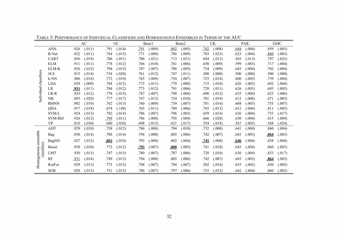
Table 5 and Table 6 report the benchmarking in terms of the AUC. We use bold face to
highlight the best performing classifier per data set. An underscore indicates that a classifier
performs best in its family (e.g., best individual classifier, best homogeneous ensemble, etc.).
Note that the performance estimates represent averages, which we compute across the multiple
random test set partitions in our Nx2 cross-validation setup (see Section 4.2). Figures in square
brackets represent the corresponding standard deviations.
Table 5 indicates that the best performing individual classifiers are, respectively, LR, SVM-
Rbf, ANN (for the Bene2, UK, and PAK data set) and B-Net. This is in line with previous results
of Baesens et al. (2003b), who also found ANN to be the best performing individual classifier in
terms of the AUC. However, we are able to extend their result in the sense that our study
incorporates different forms of extreme learning machines. These relatively new classifiers
possess several advantageous compared to ANN and RbfNN and are typically easier to use (e.g.,
Huang et al., 2006a). However, Table 5 suggests that these advantages do not translate into more
accurate predictions for the credit scoring data sets under study.
The most striking result compared to Baesens et al. (2003b) is related with ensemble
classifiers. Baesens et al. (2003b) concentrated exclusively on individual classifiers. Table 5
provides strong evidence that such classifiers are inferior to ensemble methods. In six out of
seven data sets, the overall best performing classifier belongs to the ensemble family. The only
exception is AC where LR performs slightly better than the most accurate ensemble, RF
(AUC=.9315 c.f. 0.9310).
32
TABLE 5: PERFORMANCE OF INDIVIDUAL CLASSIFIERS AND HOMOGENEOUS ENSEMBLES IN TERMS OF THE AUC AC GC Bene1 Bene2 UK PAK GMC
Indi
vidu
al c
lass
ifie
rs
ANN .926 (.011) .791 (.014) .791 (.009) .802 (.005) .742 (.008) .644 (.004) .859 (.003) B-Net .922 (.011) .764 (.015) .771 (.009) .786 (.009) .703 (.023) .623 (.004) .860 (.003) CART .856 (.019) .706 (.031) .706 (.021) .713 (.021) .684 (.012) .565 (.015) .797 (.025) ELM .911 (.011) .778 (.012) .766 (.010) .761 (.006) .650 (.009) .599 (.003) .717 (.004) ELM-K .926 (.012) .794 (.015) .787 (.007) .788 (.005) .734 (.009) .643 (.004) .702 (.004) J4.8 .915 (.014) .734 (.020) .761 (.012) .747 (.011) .500 (.000) .500 (.000) .500 (.000) k-NN .906 (.016) .772 (.010) .765 (.009) .754 (.007) .725 (.014) .600 (.005) .739 (.004) LDA .929 (.009) .784 (.012) .775 (.011) .779 (.008) .715 (.010) .626 (.003) .692 (.004) LR .931 (.011) .784 (.012) .773 (.012) .791 (.006) .720 (.011) .626 (.003) .693 (.005) LR-R .925 (.012) .778 (.015) .787 (.007) .798 (.004) .690 (.012) .635 (.004) .623 (.006) NB .893 (.020) .777 (.017) .747 (.013) .724 (.010) .701 (.019) .613 (.006) .671 (.003) RbfNN .902 (.019) .762 (.013) .760 (.009) .739 (.007) .701 (.014) .604 (.003) .755 (.007) QDA .917 (.018) .674 (.148) .765 (.011) .780 (.006) .703 (.012) .612 (.004) .811 (.003) SVM-L .924 (.013) .782 (.014) .786 (.007) .796 (.003) .659 (.014) .636 (.004) .733 (.017) SVM-Rbf .926 (.012) .799 (.011) .786 (.008) .795 (.004) .666 (.028) .630 (.004) .815 (.009) VP .810 (.030) .680 (.020) .698 (.013) .621 (.017) .554 (.018) .567 (.003) .568 (.024)
Hom
ogen
eous
ens
embl
e cl
assi
fier
s
ADT .929 (.010) .758 (.012) .786 (.008) .794 (.010) .732 (.008) .641 (.004) .860 (.004)
Bag .930 (.014) .788 (.014) .794 (.008) .805 (.006) .742 (.007) .643 (.003) .864 (.003)
BagNN .927 (.012) .802 (.010) .793 (.008) .802 (.004) .745 (.008) .646 (.004) .838 (.004)
Boost .930 (.010) .772 (.012) .795 (.007) .808 (.005) .741 (.010) .643 (.004) .860 (.003)
LMT .930 (.013) .747 (.015) .780 (.007) .787 (.006) .720 (.010) .630 (.004) .833 (.017)
RF .931 (.014) .789 (.013) .794 (.008) .805 (.006) .742 (.007) .643 (.003) .864 (.003)
RotFor .929 (.013) .773 (.015) .788 (.007) .794 (.007) .502 (.016) .635 (.002) .820 (.005)
SGB .928 (.013) .751 (.015) .786 (.007) .797 (.006) .735 (.012) .642 (.004) .860 (.003)

33
The appealing performance of the ensemble methods reemphasizes the need to update the
Baesens et al. (2003b) study. The methods that were not considered in the original study improve
predictive accuracy. This might be taken as evidence of progress in the field of predictive
modeling. One the other hand, the best performing ensemble methods are typically bagging,
boosting, and random forest. Arguably, these classifiers are well-known in credit scoring. Less
known and/or more recent ensembles such as SGB or RotFor fail to outperform their more
established counterparts such as Bag or RF. This indicates that further progress beyond Bag or
RF is difficult to achieve. It is thus interesting to explore the performance of heterogeneous
ensembles. Table 6 reports the corresponding results.
Table 6 suggests that a weighted average is often slightly better than a simple average when
combining all base model predictions. Given that we create large libraries of about 1,000 base
models, one might suspect that some base models give poor performance. Combining only a
subset of base models should thus improve predictive accuracy. However, when comparing the
results of AvgS and AvgW to Top-T, we find only moderate evidence for this suspicion. For
example, Top-T gives better performance in four out of seven cases. For comparative purpose, we
also report the performance of an extreme base model pruning where the final “ensemble”
consists only of the single best base model (BBM). This approach is typically inferior to Top-T.
Thus, considering only the four top-most ensemble strategies in Table 6, we conclude that
combining multiple (heterogeneous) classifiers increases accuracy (e.g., compared to BBM) and
that it is challenging to determine the “right” amount of pruning.
The other ensembles of Table 6 address this issue through different base model selection
strategies. With respect to direct approaches, choosing base models using the principles of
heuristic search seems to be effective. For example, HCES-Bag employs a simple hill-climbing
algorithm to select base models. Embedding this approach in a bagging framework, HCES-Bag
gives the best AUC performance among the static direct ensemble methods in five out of seven
cases. Similarly, selecting base models by means of a genetic algorithm (i.e., GASEN) produces
appealing results on all data sets and the overall best AUC performance on the GC data set. The
suitability of heuristic search also extends to the indirect ensemble selection approaches, where
we observe five wins (within the family) for UWA. This ensemble uses the same hill-climbing
algorithm as HCES and HCES-Bag for base model selection, but to maximize a different
objective.

34
TABLE 6: PERFORMANCE OF HETEROGENEOUS ENSEMBLES IN TERMS OF THE AUC AC GC Bene1 Bene2 UK PAK GMC
No ensemble selection AvgS .931 (.014) .807 (.008) .798 (.007) .806 (.004) .747 (.009) .648 (.004) .859 (.004) AvgW .931 (.014) .807 (.008) .799 (.007) .806 (.004) .748 (.009) .648 (.004) .860 (.004)
Static direct ensemble selection
Top-T .933 (.012) .799 (.010) .797 (.009) .811 (.005) .748 (.007) .649 (.004) .865 (.003) BBM .928 (.009) .795 (.012) .794 (.007) .807 (.005) .744 (.009) .645 (.004) .864 (.003) CompM .923 (.019) .787 (.018) .787 (.011) .806 (.006) .740 (.008) .644 (.004) .861 (.003) EPVRL .931 (.014) .807 (.008) .799 (.007) .806 (.004) .747 (.010) .648 (.004) .859 (.003) GASEN .931 (.014) .807 (.008) .798 (.007) .806 (.004) .748 (.009) .648 (.004) .859 (.004) HCES .931 (.013) .795 (.013) .797 (.008) .813 (.005) .746 (.008) .652 (.003) .865 (.003) HCES-Bag .933 (.013) .801 (.010) .800 (.008) .814 (.005) .749 (.008) .652 (.003) .865 (.003) MPOCE .932 (.014) .800 (.013) .798 (.007) .810 (.006) .742 (.007) .647 (.004) .861 (.003) Stack .897 (.020) .734 (.020) .754 (.014) .793 (.005) .692 (.034) .648 (.004) .861 (.003)
Static indirect ensemble selection
CuCE .932 (.013) .798 (.014) .796 (.008) .809 (.004) .746 (.007) .650 (.004) .856 (.009) k-Means .927 (.016) .802 (.011) .795 (.009) .808 (.004) .744 (.011) .648 (.004) .861 (.004) KaPru .769 (.302) .744 (.032) .719 (.048) .765 (.043) .730 (.012) .640 (.005) .831 (.009) MDM .926 (.017) .789 (.015) .792 (.006) .800 (.006) .742 (.007) .637 (.005) .861 (.003) UWA .933 (.013) .801 (.011) .800 (.008) .814 (.005) .747 (.007) .645 (.004) .862 (.004)
Dynamic ensemble selection
kNORA .904 (.013) .772 (.014) .767 (.010) .779 (.003) .746 (.010) .643 (.003) .559 (.146)
PMCC .860 (.013) .610 (.026) .637 (.011) .615 (.011) .500 (.000) .500 (.000) n.A.*
* PMCC exhausted the available main memory of 64GB and failed to produce a valid ensemble.

35
A common denominator of Table 5 and Table 6 is that ensemble methods work well in
general. However, we also observe that more recent and/or more complex ensemble strategies do
not necessarily perform better than simpler ensembles. This view is also supported by the results
of the two dynamic ensemble selection approaches. Dynamic selection is conceptually more
complex than static ensemble selection, because an individual ensemble is formed for every case
of the test set. However, the two dynamic ensemble selection techniques, KNORA and PMCC,
perform much worse than static selection approaches, including the very simple approach to
average all base model predictions (i.e. AvgS).
5.2 Correspondence of predictive accuracy across performance measures
The results of the other performance measures (PCC, BS, H-measure) show a similar
tendency as the results in terms of the AUC. Interested readers find the corresponding figures in
Appendix II. A summary of the results of all performance measures is provided in Table 7 and
Table 8 for individual/homogeneous ensemble classifiers and heterogeneous ensemble classifiers,
respectively. In particular, we report for each performance measure the average rank of the
classifiers across all data sets. For example, a classifier that performs best across all data sets
receives an average rank of one. Accordingly, a classifier that performs best on three and second-
best on four data sets receives an average rank of (3*1+4*2)/7= 1.57. The last column in Table 7
and Table 8 gives the grand average across all performance measures.
With respect to individual classifiers and homogeneous ensembles, Table 7 reveals that RF
performs best. RF achieves the lowest average rank, no matter whether we assess predictive
accuracy in terms of the AUC, PCC, BS, or the H-measure. In addition, Table 7 further supports
the view that ensemble classifiers perform typically better than individual classifiers. Across the
four performance measures, the three most accurate classifiers (RF, BagNN, Bag) belong to the
ensemble family. To some extent, their advantage is due to increased robustness compared to
individual classifiers. For example, LR achieves an average rank of 5.17 (third best classifier) in
terms of the BS. However, other performance measures draw a different picture. Average ranks
of around 11 for LR indicate only moderate performance. We observe a similar trend for ANN.
The ANN classifier performs rather well in terms of the AUC but very poorly in terms of the BS.
However, it is important to acknowledge that not all ensembles exhibit robustness toward
different performance measures. For example, LMT performs well in terms of BS but poorly in
terms of the other performance measures, whereas boosting shows the opposite trend. The two

36
bagging classifiers and especially RF, on the other hand, perform very stable across different
performance measures.
TABLE 7: AVERAGE RANKS OF INDIVIDUAL CLASSIFIERS AND HOMOGENEOUS ENSEMBLES AvgR-AUC AvgR-PCC AvgR-BS AvgR-H-Measure AvgR
Indi
vidu
al c
lass
ifie
rs
ANN 5.95 (.6505) 7.93 (.1008) 14.17 (.0000) 6.88 (.0377) 8.73 B-Net 14.25 (.0000) 13.49 (.0000) 8.90 (.0000) 14.38 (.0000) 12.75 CART 21.52 (.0000) 19.18 (.0000) 21.07 (.0000) 21.01 (.0000) 20.70 ELM 16.91 (.0000) 16.93 (.0000) 22.65 (.0000) 16.75 (.0000) 18.31 ELM-K 8.49 (.0009) 8.83 (.0108) 22.57 (.0000) 8.16 (.0008) 12.01 J4.8 20.17 (.0000) 17.30 (.0000) 10.67 (.0000) 19.16 (.0000) 16.82 k-NN 16.43 (.0000) 17.22 (.0000) 14.84 (.0000) 17.04 (.0000) 16.38 LDA 12.05 (.0000) 10.85 (.0000) 7.23 (.0004) 11.56 (.0000) 10.42 LR 11.03 (.0000) 10.46 (.0000) 5.17 (.1556) 10.69 (.0000) 9.34 LR-R 11.44 (.0000) 11.07 (.0000) 18.44 (.0000) 11.49 (.0000) 13.11 NB 18.06 (.0000) 17.99 (.0000) 13.30 (.0000) 18.34 (.0000) 16.92 RbfNN 18.03 (.0000) 18.35 (.0000) 15.68 (.0000) 18.51 (.0000) 17.64 QDA 17.57 (.0000) 16.96 (.0000) 9.34 (.0000) 17.72 (.0000) 15.40 SVM-L 11.51 (.0000) 12.00 (.0000) 17.54 (.0000) 11.99 (.0000) 13.26 SVM-Rbf 9.68 (.0000) 10.46 (.0000) 18.22 (.0000) 9.98 (.0000) 12.08 VP 23.23 (.0000) 23.15 (.0000) 19.94 (.0000) 23.28 (.0000) 22.40
Hom
ogen
eous
ens
embl
e cl
assi
fier
s
ADT 9.45 (.0000) 8.58 (.0203) 4.66 (.3003) 9.01 (.0000) 7.92 Bag 4.85 (.9471) 6.07 (.6868) 7.21 (.0004) 4.43 (.9025) 5.64
BagNN 4.76 (.9471) 6.44 (.6868) 3.57 (.7019) 5.26 (.7007) 5.01
Boost 6.10 (.6298) 7.40 (.2678) 13.01 (.0000) 6.85 (.0377) 8.34 LMT 12.48 (.0000) 12.48 (.0000) 6.11 (.0153) 13.08 (.0000) 11.04 RF 4.69 / 5.66 / 3.18 / 4.31 / 4.46 RotFor 11.35 (.0000) 10.94 (.0000) 13.28 (.0000) 10.07 (.0000) 11.41 SGB 10.00 (.0000) 10.23 (.0001) 9.25 (.0000) 10.05 (.0000) 9.88
Friedman 1323.61 (.0000) 1026.72 (.0000) 1654.40 (.0000) 1298.26 (.0000) Values in brackets represent the adjusted p-value corresponding to a pairwise comparison of the row classifier
to RF. Bold face indicates significance at the 5%, an underscore significance at the 1% level. To account for the overall number of pairwise comparisons, we adjust p-values using the Rom-procedure (García et al., 2010). Prior to conducting multiple comparisons, we employ the Friedman test to verify that at least two classifiers perform significantly different (e.g., Demšar, 2006). The last row shows the corresponding and p-values.
The average ranks in Table 7 are also the basis for statistical testing. We consider
nonparametric testing procedures because these are most suitable for classifier comparisons
across multiple data sets (e.g., Demšar, 2006; García et al., 2010). First, we employ the Friedman
test to test the null-hypothesis that the average ranks of all classifiers are statistically equivalent,
against the alternative hypothesis that at least two classifiers differ. The test statistic is
distributed with k-1 degrees of freedom, where k denotes the number of classifiers. The last row
of Table 7 depicts the empirical values of the test statistic. The corresponding p-values (shown in
square brackets in the last row) suggest that we can reject the hull-hypothesis for all performance

37
measures with high confidence. This allows us to proceed with multiple-comparisons to identify
which classifiers perform significantly different. In particular, we perform 23 pairwise
comparisons of one classifier and RF. The latter performs best and serves as control classifier in
the comparison (e.g., García et al., 2010). Thus, each pairwise comparison tests the null-
hypothesis that a classifier is statistically equivalent to RF. Table 7 shows the adjusted p-values
corresponding to these tests for all classifiers and performance measures (in square-brackets).
Note that an adjustment of p-values is crucial to control the family-wise error level when testing
multiple hypotheses (e.g., Demšar, 2006). We follow the recommendation of García et al. (2010)
and use the Rom-procedure for p-value adjustment.
The statistical analysis indicates that individual classifiers predict – with few exceptions –
significantly less accurately than RF. The only cases where we lack sufficient evidence to reject
the null-hypothesis are ANN (on AUC and PCC) and LR (on BS). The results are less clear
among the homogeneous ensemble classifiers. It is typically not possible to reject the null-
hypothesis of equal performance between RF and the strongest competitors, BagNN and Bag.
Other homogeneous ensemble classifiers perform less competitive and predict significantly less
accurately than RF in many cases. It is noteworthy that RF performs significantly better than
RotFor. RotFor can be considered a successor of RF and has shown promising performance in
previous experiments in other domains (e.g., Rodriguez et al., 2006). However, as in the previous
comparison of ANN versus ELM, we once again observe no evidence that the successor beats the
predecessor in credit scoring.
The ranking results for heterogeneous ensembles across the four performance measures are
shown in Table 8. The clear winner among the heterogeneous ensembles is HCES-Bag (Caruana
et al., 2006). It achieves the lowest (best) average rank across all performance measures.
Moreover, the p-values of the pairwise comparisons to other heterogeneous ensembles reveal that
HCES-Bag predicts significantly more accurate than most of its competitors. It is also noteworthy
that the runner-up in the comparison is HCES, which is just a simplified version of HCES-Bag.

38
TABLE 8: AVERAGE RANKS OF HETEROGENEOUS ENSEMBLE CLASSIFIERS AvgR-AUC AvgR-PCC AvgR-BS AvgR-H-measure AvgR
No ensemble selection
AvgS 7.21 (.0004) 7.59 (.0333) 5.90 (.0155) 7.14 (.0807) 6.96 AvgW 6.05 (.0152) 8.16 (.0052) 7.20 (.0001) 5.61 (.6313) 6.76
Static direct ensemble selection
Top-T 6.16 (.0152) 8.75 (.0003) 8.27 (.0000) 6.66 (.1980) 7.46 BBM 10.04 (.0000) 9.58 (.0000) 9.13 (.0000) 9.99 (.0000) 9.68 CompM 11.77 (.0000) 9.49 (.0000) 17.10 (.0000) 11.20 (.0000) 12.39 EPVRL 6.77 (.0028) 7.69 (.0275) 6.01 (.0145) 7.41 (.0349) 6.97 GASEN 7.35 (.0002) 7.54 (.0333) 6.11 (.0120) 6.88 (.1635) 6.97 HCES 6.35 (.0149) 7.27 (.0551) 5.54 (.0271) 6.73 (.1980) 6.47 HCES-Bag 4.14 / 5.52 / 3.83 / 5.24 / 4.68 MPOCE 7.46 (.0001) 7.22 (.0551) 7.59 (.0000) 7.40 (.0349) 7.42 Stack 14.80 (.0000) 13.58 (.0000) 16.96 (.0000) 14.58 (.0000) 14.98
Static indirect ensemble selection
CuCE 7.45 (.0001) 7.71 (.0275) 8.27 (.0000) 7.84 (.0071) 7.82 k-Means 8.59 (.0000) 8.06 (.0076) 7.87 (.0000) 7.59 (.0197) 8.03 KaPru 15.77 (.0000) 14.72 (.0000) 11.20 (.0000) 15.90 (.0000) 14.40 MDM 12.40 (.0000) 11.17 (.0000) 8.34 (.0000) 11.72 (.0000) 10.91 UWA 6.00 (.0152) 6.89 (.0755) 11.57 (.0000) 6.46 (.2275) 7.73
Dynamic ensemble selection
KNORA 14.79 (.0000) 14.08 (.0000) 15.19 (.0000) 15.00 (.0000) 14.76
PMCC 17.91 (.0000) 15.97 (.0000) 14.91 (.0000) 17.66 (.0000) 16.61
Friedman 945.1 (.0000) 559.0 (.0000) 953.5 (.0000) 867.3 (.0000)
Table 8 facilitates some conclusions concerning the relative effectiveness of different
ensemble selection strategies. First, we observe strong evidence that dynamic ensemble selection
strategies are less suitable in credit scoring. At least the representatives we consider, KNORA
and PMCC, perform worse than several other, typically much simpler classifiers.
Second, ensemble selection strategies that pursue an indirect optimization of ensemble
performance (e.g., through maximizing diversity during selection) do not improve performance
compared to ensembles without base model selection. Considering the result across all
performance measures (last column of Table 8), both AvgS and AvgW achieve lower average
ranks than the indirect ensemble selection strategies. This finding echoes previous concerns that
the link between diversity and ensemble performance is intricate and difficult to exploit in an
ensemble modeling framework (e.g., Tang et al., 2006). However, we acknowledge that our
result is to some extent influenced by the poor performance of UWA in terms of the BS. In terms
of the AUC, PCC, and H-measure, UWA performs at least competitive to AvgS and AvgW.
Third, we find some evidence that direct selection strategies might be more effective than
indirect selection strategies. However, drawing a final conclusion on that matter appears
premature. Some direct ensembles (e.g., HCES-Bag) perform very well, whereas others perform

39
worse than indirect ensembles or full ensembles without selection (e.g., Stack and ComP). In that
sense, we conclude that an additional selection of base models can improve ensemble
performance (e.g., compared to averaging over all available base models). However, selecting the
‘right’ base models for an ensemble seems a nontrivial task with many pitfalls. For the retail
credit scoring data sets under study, we conclude that a direct hill-climbing selection of base
models is an effective approach to develop accurate heterogeneous ensemble classifiers from
libraries of models.
Independent from the relative performance of competing classifiers, Table 7 and Table 8 also
shed some light on the degree to which alternative performance measures differ in their classifier.
To get a clearer view on this issue, Table 9 depicts the correlation of the classifier rankings across
the four performance measures in terms of Kendall’s rank correlation coefficient. We observe
relatively large agreement between the results belonging to the PCC, AUC, and H-measure. This
is especially true for individual classifiers and homogeneous ensembles, and, to lesser extent also
for heterogeneous ensembles. On the one hand, this suggests that it may be dispensable to use
these performance measures together in a single comparison.
A more important finding concerns the high correlation between the AUC and H-measure
results. The AUC depends on the score distribution of a classifier and does, for this reasons,
assesses alternative classifiers in an incoherent manner (Hand & Anagnostopoulos, 2013).
However, Table 9 indicates that this conceptual shortcoming does not affect the results of
empirical classifier comparisons to a large extent. Ranking classifiers in terms of the H-measure
gives almost the same result as if using the AUC. Thus, if a credit analyst were to choose a
scorecard among several alternatives, the AUC and the H-measure would typically give the same
recommendation. On the one hand, this suggests that it is safe to continue using the AUC for
scorecard comparisons. On the other hand, one could argue that there is little reason to do so,
given that a conceptually more appropriate measure is readily available.
Finally, Table 9 suggests that the BS differs more substantially from the other performance
measures. The BS is the only indicator that assesses the accuracy of the estimated default
probabilities. This provides some insight whether the model estimates are well calibrated, which
is an important issue in credit scoring (e.g., Blochlinger & Leippold, 2011). Moreover, moderate
correlation with other performance measures suggest that the notion of model performance
embodied in the BS contributes some valuable information to a classifier benchmark.

40
Consequently, we recommend that future studies should routinely use the BS alongside other,
more established5 performance measures to assess alternative scorecards.
TABLE 9: CORRELATION OF CLASSIFIER RANKINGS ACROSS PERFORMANCE INDICATORS
Individual classifier &
homogeneous ensembles Heterogeneous ensembles
AUC PCC BS H AUC PCC BS H AUC 1.00 1.00 PCC .913 1.00 .686 1.00 BS .341 .399 1.00 .538 .551 1.00
H .957 .942 .341 1.00 .895 .739 .538 1.00
Correlation is measured terms of Kendall’s rank correlation coefficient.
5.3 Comparison of selected scoring techniques
Having compared a large number of classifiers to each other, a natural question arising is
whether we can identify one single best approach. To shed light on this issue we select the three
best performing classifiers of each category (single classifiers, homogeneous ensemble classifier,
heterogeneous ensembles) and LR (because of this popularity in credit scoring) and compare their
performance in Table 10. More specifically, we compute the average rank of every classifier
across all data sets and performance measure (second column of Table 10). Overall, HCES-Bag
gives the most accurate predictions, followed by RF, ANN, and LR. We use the Friedman test to
check whether at least two classifiers perform significantly different. The last row of Table 10
shows the empirical value of the test statistic. Based on the observed value of 141.51, we
reject the null-hypothesis (p-value < 0.000) and proceed with multiple comparisons. More
specifically, we perform six multiple comparisons to contrast all classifiers against each other.
We control the family-wise error level using the Bergmann-Hommel procedure (e.g., García et
al., 2010). Table 10 depicts the adjusted p-values. Based on the observed results, we conclude
that i) LR predicts significantly less accurately than any of the other classifiers, that ii) the
empirical results do not provide sufficient evidence to conclude whether RF and ANN perform
significantly different, and that iii) HCES-Bag predicts significantly more accurate than LR,
ANN, and RF. This result further supports the view that HCES-Bag is well-suited to create
accurate retail scorecards.
5 Recall that none of the studies in Table 1 employ the BS.

41
TABLE 10: STATISTICAL COMPARISON OF SELECTED CLASSIFIERS
AvgR Adjusted p-values of pairwise comparisons
ANN LR RF ANN 2.37 LR 3.09 .0000 RF 2.54 .0736 .0000 HCES-Bag 2.00 .0001 .0000 .0000
Friedman 141.51 (.0000)
6 Conclusions
We set out to update the study of Baesens et al. (2003b) and to explore the relative
effectiveness of alternative classification algorithms in retail credit scoring. To that end, we
compared the predictive performance of 41 classifiers in terms of the PCC, AUC, BS, and H-
measure using a set of seven real-world credit scoring data sets. Our results agree with Baesens et
al. (2003b) in that artificial neural networks are a powerful individual classifier. Unlike Baesens
et al. (2003b), we found that neural networks predict PD significantly more accurately than the
industry standard, logistic regression. We argue that this discrepancy is due to using a more
powerful statistical testing framework and an extended Nx2 cross-validation design for this study.
In addition, we observed a tendency that homogenous ensemble classifiers outperform individual
classifiers. Among these two groups, the five best performing methods belong to the
homogeneous ensemble family, with RF giving the most accurate PD estimates. Finally, we
observed the overall best results for an ensemble selection approach that integrates the principles
of bootstrap sampling with a greedy hill-climbing algorithm for base model selection (Caruana et
al., 2006). In particular, the HCES-Bag classifier performed significantly better than random
forest, feed-forward neural networks, or logistic regression.
Our study consolidates pervious work in PD modeling and provides a holistic picture of the
state-of-the-art in predictive modeling for retail scorecard development. This has implications for
both academics and researchers in credit scoring. From an academic point of view, an important
question is to what extent novel classifiers give better performance. This helps to judge whether
efforts into the development of novel scoring techniques are worthwhile. From a managerial
perspective, the key question is whether the winning classifiers of our comparison can and should
be adopted in corporate practice.
With respect to developing novel classification algorithms, our results offer some supporting
conclusions but also raise some concerns. On the one hand, we find some advanced methods to

42
perform extremely well on our credit scoring data sets. On the other hand, we observe several
sophisticated techniques such as rotation forests or dynamic ensemble selection to predict PD less
accurately than logistic regression. Moreover, we never observe one of the latest developments in
the field to give the best result in the groups of individual classifiers, homogeneous ensembles,
and heterogeneous ensembles. Standard feed-forward neural networks perform better than
extreme learning machines, random forest better than rotation forest, and the HCES-Bag
classifier better than any other heterogeneous ensemble classifier considered in the study. This
could suggest that progress in the field has stalled (e.g., Hand, 2006).
Despite the previous concern, we do not expect the desire to develop better, more accurate
scorecards to end any time soon. Likely, future papers will propose novel classifiers and the
“search for the silver bullet” (Thomas, 2010) will continue. An important implication of our
study is that such efforts must be accompanied by a rigorous assessment of the proposed method
vis-à-vis challenging reference classifiers. In particular, we recommend random forest as a
reference benchmark against which to compare new classification algorithms in retail credit
scoring. HCES-Bag would be an even more challenging benchmark, but is not as easily available
as random forest (e.g., in standard data mining software). Moreover, we suggest that the practice
of comparing a newly proposed classifier to logistic regression (and/or some other established
individual classifier) only, which we still observe in the credit scoring literature, should be
avoided. Clearly logistic regression is the industry standard (e.g., Crook et al., 2007). It is useful
to examine how a new classifier compares to this standard as well as to other established
techniques. However, given the state-of-the-art in predictive modeling, outperforming logistic
regression can no longer be accepted as signal for a methodological advancement; but
outperforming random forest can.
A related implication concerns the organization of empirical classifier comparisons.
Predictive performance can vary considerably across different accuracy indicators. For example,
logistic regression gave medium performance on average but performed better than most
competitors in terms of the BS. More generally, we observed a trend that the PCC, AUC, and H-
measure agree to a large extent, whereas the BS is less correlated with the other measures.
Therefore, the BS offers an additional angle from which to examine the predictive performance
of a scorecard. However, none of the PD modeling papers we examined in the literature review
employs the BS. In the light of our results, this is another practice that deserves revision. Future

43
studies that propose a new scoring technique should routinely consider the BS alongside more
popular measures such as the PCC to obtain a clearer view how the new classifier performs.
From a managerial perspective, it is important to reason whether the appealing performance
of random forest or HCES-Bag generalizes to real-world applications and what returns would
result from such performance improvements. This question is much debated in the literature.
Finlay (2011) provides an insightful discussion on the matter. In brief, supporters of advanced
techniques argue that small improvements in predictive accuracy translate into sizeable financial
rewards (e.g., Baesens et al., 2003b; Thomas et al., 2002; West et al., 2005). Opponents of
advanced methods reject this view. They argue that benchmarking studies (such as this one)
overestimate the advantages of novel classifiers for various reasons (e.g., Gayler, 2006; Hand,
2006). Further criticism is associated with the lack of organizational acceptance and compliance
with regulatory frameworks such as Basel II, because advanced methods are opaque and difficult
to interpret. Supporters reply to this criticism by referring to rule extraction techniques that
explain the mechanisms of some complex classifier in an easy understandable manner (e.g.,
Baesens et al., 2003a; Hoffmann et al., 2007; Martens et al., 2007).
From this study, we can add some points to the discussion on the pros and cons of advanced
classifiers in retail credit scoring. As we demonstrate in this work, advancements in computer
power, classifier learning, and statistical testing facilitate more rigorous comparisons compared to
previous studies. Clearly, this does not guarantee external validity. Several concerns why
laboratory experiments (as this one) overestimate the advantage of advanced classifiers in credit
scoring (e.g., Hand, 2006) remain valid; and maybe insurmountable. However, experimental
designs with several cross-validation repetitions, different performance measures and appropriate
multiple-comparison procedures overcome some important limitations of previous studies and,
thereby, provide stronger support that advanced scoring techniques have the potential to
outperform present solutions and logistic regression in particular in real-world settings.
In addition, our results facilitate some remarks related with the organizational acceptance of
advanced classifiers (or the lack thereof). When developing a classification model, we
deliberately avoided manual tuning. The performance differences that we observe result from a
fully-automatic modeling. One could argue that automation does not improve the organizational
acceptance of advanced scoring techniques and, in fact, decreases managers’ acceptance of such
decision support models. However, the ability of some advanced techniques to predict
significantly more accurately than simpler classifiers and logistic regression in particular

44
mitigates concerns that much expertise is needed to master advanced classifiers. This is not the
case. For example, our results evidence that a random forest classifier, which (automatically)
tests some standard meta-parameter settings from the literature, produces very competitive retail
scorecards.
Finally, an even more important question concerns the business value of advanced classifiers.
In general, the degree to which monetary returns emerge out of increased predictive accuracy will
depend on the number of business decisions that scorecards are meant to support. The task to
score retail credits is part of operational management. A vast number of decisions have to be
made every day and the financial consequences of an individual decision are comparably small.
An automation of decision processes is often unavoidable in the retail business; for example in
the credit card business or online-applications where sellers offer various payment options or
financing plans to almost anonymous customers. Moreover, novel forms of money lending such
as peer-to-peer lending gain momentum (e.g., Lin et al., 2013) and may have a substantial impact
on the retail credit business in the future. Such operational settings with a high frequency of
decision tasks are exactly the environment where higher (statistical) accuracy translates into
business value. One-time investments (e.g., for hardware, software, and user training) into a more
elaborate scoring technique will pay-off in the longer run when small but significant accuracy
improvements are multiplied by hundreds of thousands of scorecard applications.
Regulatory frameworks and organization acceptance constrain and sometimes prohibit the use
of advance scoring today; at least for classic credit products. However, considering the shift
toward a data-driven decision making paradigm, which current industry trends such as big data,
customer intelligence, or advanced analytics embody, and the richness of online-mediated forms
of credit granting, we foresee a bright future for advanced scoring methods in academia and
industry.
References
Abdou, H., Pointon, J., & El-Masry, A. (2008). Neural nets versus conventional techniques in credit scoring in Egyptian banking. Expert Systems with Applications, 35(3), 1275-1292.
Abdou, H.A. (2009). Genetic programming for credit scoring: The case of Egyptian public sector banks. Expert Systems with Applications, 36(9), 11402-11417.
Akkoc, S. (2012). An empirical comparison of conventional techniques, neural networks and the three stage hybrid Adaptive Neuro Fuzzy Inference System (ANFIS) model for credit scoring analysis: The case of Turkish credit card data. European Journal of Operational Research, 222(1), 168-178.

45
Asuncion, A., & Newman, D.J. (2010). UCI Machine Learning Repository. In: School of Information and Computer Science, University of California, Irvine, CA.
Atish, P.S., & Jerrold, H.M. (2004). Evaluating and tuning predictive data mining models using receiver operating characteristic curves. Journal of Management Information Systems, 21(3), 249-280.
Baesens, B., Setiono, R., Mues, C., & Vanthienen, J. (2003a). Using neural network rule extraction and decision tables for credit-risk evaluation. Management Science, 49(3), 312-329.
Baesens, B., Van Gestel, T., Viaene, S., Stepanova, M., Suykens, J., & Vanthienen, J. (2003b). Benchmarking state-of-the-art classification algorithms for credit scoring. Journal of the Operational Research Society, 54(6), 627-635.
Banasik, J., & Crook, J. (2007). Reject inference, augmentation, and sample selection. European Journal of Operational Research, 183(3), 1582-1594.
Banasik, J., Crook, J., & Thomas, L.C. (2003). Sample selection bias in credit scoring models. Journal of the Operational Research Society, 54(8), 822-832.
Banfield, R.E., Hall, L.O., Bowyer, K.W., & Kegelmeyer, W.P. (2005). Ensemble diversity measures and their application to thinning. Information Fusion, 6(1), 49-62.
Bellotti, T., & Crook, J. (2009a). Support vector machines for credit scoring and discovery of significant features. Expert Systems with Applications, 36(2), 3302–3308.
Bellotti, T., & Crook, J. (2012). Loss given default models incorporating macroeconomic variables for credit cards. International Journal of Forecasting, 28(1), 171-182.
Bellotti, T., & Crook, J.N. (2009b). Credit scoring with macroeconomic variables using survival analysis. Journal of the Operational Research Society, 60, 1699–1707.
Blochlinger, A., & Leippold, M. (2011). A new goodness-of-fit test for event forecasting and its application to credit defaults. Management Science, 57(3), 487-505.
Boylu, F., Aytug, H., & Koehler, G.J. (2010). Induction over constrained strategic agents. European Journal of Operational Research, 203(3), 698-705.
Bravo, C., Maldonado, S., & Weber, R. (2013). Granting and managing loans for micro-entrepreneurs: New developments and practical experiences. European Journal of Operational Research(0).
Breiman, L. (1996a). Bagging predictors. Machine Learning, 24(2), 123-140.
Breiman, L. (1996b). Stacked regressions. Machine Learning, 24(1), 49-64.
Breiman, L. (2001). Random forests. Machine Learning, 45(1), 5-32.
Brown, I., & Mues, C. (2012). An experimental comparison of classification algorithms for imbalanced credit scoring data sets. Expert Systems with Applications, 39(3), 3446-3453.
Caruana, R., Munson, A., & Niculescu-Mizil, A. (2006). Getting the Most Out of Ensemble Selection. In Proc. of the 6th Intern. Conf. on Data Mining (pp. 828-833). Hong Kong, China: IEEE Computer Society.
Caruana, R., & Niculescu-Mizil, A. (2006). An Empirical Comparison of Supervised Learning Algorithms. In W. W. Cohen & A. Moore (Eds.), Proc. of the 23rd Intern. Conf. on Machine Learning (pp. 161-168). Pittsburgh, Pennsylvania, USA: ACM.
Caruana, R., Niculescu-Mizil, A., Crew, G., & Ksikes, A. (2004). Ensemble Selection from Libraries of Models. In C. E. Brodley (Ed.), Proc. of the 21st Intern. Conf. on Machine Learning (pp. 18-25). Banff, Alberta, Canada: ACM.
Chang, C.-C., & Lin, C.-J. (2001). LIBSVM - A Library for Support Vector Machines. In.
Chen, W., Ma, C., & Ma, L. (2009). Mining the customer credit using hybrid support vector machine technique. Expert Systems with Applications, In Press, Accepted Manuscript.
Chih-Jen, L., Ruby, C.W., & Keerthi, S.S. (2008). Trust region newton methods for large-scale logistic regression. Journal of Machine Learning Research, 9, 627-650.

46
Crone, S.F., Lessmann, S., & Stahlbock, R. (2006). The impact of preprocessing on data mining: An evaluation of classifier sensitivity in direct marketing. European Journal of Operational Research, 173(3), 781-800.
Crook, J.N., Edelman, D.B., & Thomas, L.C. (2007). Recent developments in consumer credit risk assessment. European Journal of Operational Research, 183(3), 1447-1465.
De Andrade, F.W.M., & Thomas, L. (2007). Structural models in consumer credit. European Journal of Operational Research, 183(3), 1569-1581.
Demšar, J. (2006). Statistical comparisons of classifiers over multiple data sets. Journal of Machine Learning Research, 7, 1-30.
Dietterich, T.G. (1998). Approximate statistical tests for comparing supervised classification learning. Neural Computation, 10(7), 1895-1923.
Falangis, K., & Glen, J.J. (2010). Heuristics for feature selection in mathematical programming discriminant analysis models. Journal of the Operational Research Society, 61(5), 804-812.
Fan, R.-E., Chang, K.-W., Hsieh, C.-J., Wang, X.-R., & Lin, C.-J. (2008). LIBLINEAR: A library for large linear classification. Journal of Machine Learning Research, 9, 1871-1874.
Fawcett, T. (2006). An introduction to ROC analysis. Pattern Recognition Letters, 27(8), 861-874.
Fethi, M.D., & Pasiouras, F. (2010). Assessing bank efficiency and performance with Operational Research and Artificial Intelligence techniques: A survey. European Journal of Operational Research, 204(2), 189-198.
Finlay, S. (2011). Multiple classifier architectures and their application to credit risk assessment. European Journal of Operational Research, 210(2), 368-378.
Flach, P.A., Hernández-Orallo, J., & Ramirez, C.F. (2011). A Coherent Interpretation of AUC as a Measure of Aggregated Classification Performance. In L. Getoor & T. Scheffer (Eds.), Proc. of the 28th Intern. Conf. on Machine Learning (pp. 657-664). Bellevue, WA, USA: Omnipress.
Florez-Lopez, R. (2010). Effects of missing data in credit risk scoring. A comparative analysis of methods to achieve robustness in the absence of sufficient data. Journal of the Operational Research Society, 61(3), 486-501.
Freund, Y., & Mason, L. (1999). The Alternating Decision Tree Learning Algorithm. In I. Bratko & S. Dzeroski (Eds.), Proc. of the 16th Intern. Conf. on Machine Learning (pp. 124-133). Bled, Slovenia: Morgan Kaufmann
Freund, Y., & Schapire, R.E. (1996). Experiments With a New Boosting Algorithm. In L. Saitta (Ed.), Proc. of the 13th Intern. Conf. on Machine Learning (pp. 148-156). Bari, Italy: Morgan Kaufmann.
Freund, Y., & Schapire, R.E. (1999). Large margin classification using the perceptron algorithm Machine Learning, 37(3), 277-296.
Friedman, J.H. (2002). Stochastic gradient boosting. Computational Statistics & Data Analysis, 38(4), 367-378.
García, S., Fernández, A., Luengo, J., & Herrera, F. (2010). Advanced nonparametric tests for multiple comparisons in the design of experiments in computational intelligence and data mining: Experimental analysis of power. Information Sciences, 180(10), 2044-2064.
García, S., & Herrera, F. (2008). An extension on "Statistical comparisons of classifiers over multiple data sets" for all pairwise comparisons. Journal of Machine Learning Research, 9, 2677-2694.
Gayler, R.W. (2006). Comment: Classifier technology and the illusion of progress—credit scoring. Statistical Science, 21(1), 19-23.
Giacinto, G., Roli, F., & Fumera, G. (2000). Design of Effective Multiple Classifier Systems by Clustering of Classifiers. In Proc. of the 15th Intern. Conf. on Pattern Recognition (pp. 160 - 163). Barcelona, Spain: IEEE Computer Society.
Guang-Bin, H., Lei, C., & Chee-Kheong, S. (2006). Universal approximation using incremental constructive feedforward networks with random hidden nodes. IEEE Transactions on Neural Networks, 17(4), 879-892.
Hájek, P. (2011). Municipal credit rating modelling by neural networks. Decision Support Systems, 51(1), 108-118.

47
Hall, M., Frank, E., Holmes, G., Pfahringer, B., Reutemann, P., & Witten, I.H. (2009). The WEKA data mining software: An update. SIGKDD Explorations Newsletter, 11(1), 10-18.
Hall, M.A. (2000). Correlation-Based Feature Selection for Discrete and Numeric Class Machine Learning. In P. Langley (Ed.), Proc. of the 17th Intern. Conf. on Machine Learning (pp. 359-366). Stanford, CA, USA: Morgan Kaufmann
Hand, D.J. (1997). Construction and Assessment of Classification Rules. Chichester: John Wiley.
Hand, D.J. (2006). Classifier technology and the illusion of progress. Statistical Science, 21(1), 1-14.
Hand, D.J. (2009). Measuring classifier performance: A coherent alternative to the area under the ROC curve. Machine Learning, 77(1), 103-123.
Hand, D.J., & Anagnostopoulos, C. (2013). When is the area under the receiver operating characteristic curve an appropriate measure of classifier performance? Pattern Recognition Letters, 34(5), 492-495.
Hand, D.J., & Henley, W.E. (1997). Statistical classification models in consumer credit scoring: A review. Journal of the Royal Statistical Society: Series A (General), 160(3), 523-541.
Hand, D.J., Sohn, S.Y., & Kim, Y. (2005). Optimal bipartite scorecards. Expert Systems with Applications, 29(3), 684-690.
Harris, T. (2013). Quantitative credit risk assessment using support vector machines: Broad versus Narrow default definitions. Expert Systems with Applications, 40(11), 4404-4413.
Hastie, T., Tibshirani, R., & Friedman, J.H. (2009). The Elements of Statistical Learning (2nd ed.). New York: Springer.
He, J., Shi, Y., & Xu, W. (2004). Classifications of Credit Cardholder Behavior by Using Multiple Criteria Non-linear Programming. In Y. Shi, W. Xu & Z. Chen (Eds.), Data Mining and Knowledge Management, Chinese Academy of Sciences Symposium (Vol. 3327, pp. 154-163). Beijing, China: Springer.
Hens, A.B., & Tiwari, M.K. (2012). Computational time reduction for credit scoring: An integrated approach based on support vector machine and stratified sampling method. Expert Systems with Applications, 39(8), 6774-6781.
Hoffmann, F., Baesens, B., Mues, C., Van Gestel, T., & Vanthienen, J. (2007). Inferring descriptive and approximate fuzzy rules for credit scoring using evolutionary algorithms. European Journal of Operational Research, 177(1), 540-555.
Hsieh, N.-C., & Hung, L.-P. (2010). A data driven ensemble classifier for credit scoring analysis. Expert Systems with Applications, 37(1), 534-545.
Huang, C.-L., Chen, M.-C., & Wang, C.-J. (2007). Credit scoring with a data mining approach based on support vector machines. Expert Systems with Applications, 33(4), 847-856.
Huang, G.-B., Wang, D., & Lan, Y. (2011). Extreme learning machines: A survey. International Journal of Machine Learning and Cybernetics, 2(2), 107-122.
Huang, G.-B., Zhou, H., Ding, X., & Zhang, R. (2012). Extreme learning machine for regression and multiclass classification. IEEE Transactions on Systems, Man and Cybernetics, Part B, 42(2), 513-529.
Huang, G.-B., Zhu, Q.-Y., & Siew, C.-K. (2006a). Extreme learning machine: Theory and applications. Neurocomputing, 70(1-3), 489-501.
Huang, Y.-M., Hunga, C.-M., & Jiau, H.C. (2006b). Evaluation of neural networks and data mining methods on a credit assessment task for class imbalance problem. Nonlinear Analysis: Real World Applications, 7(4), 720-747.
Khashman, A. (2010). Neural networks for credit risk evaluation: Investigation of different neural models and learning schemes. Expert Systems with Applications, 37(9), 6233-6239.
Kiefte, M. (1999). Discriminant Analysis Toolbox In (Vol. 2007).
Kim, H.S., & Sohn, S.Y. (2010). Support vector machines for default prediction of SMEs based on technology credit. European Journal of Operational Research, 201(3), 838-846.
48
Kim, Y., & Sohn, S.Y. (2008). Random effects model for credit rating transitions. European Journal of Operational Research, 184(2), 561-573.
Ko, A.H.R., Sabourin, R., & Britto, J.a.S. (2008). From dynamic classifier selection to dynamic ensemble selection. Pattern Recognition, 41(5), 1735-1748.
Kruppa, J., Schwarz, A., Arminger, G., & Ziegler, A. (2013). Consumer credit risk: Individual probability estimates using machine learning. Expert Systems with Applications, 40(13), 5125-5131.
Kumar, P.R., & Ravi, V. (2007). Bankruptcy prediction in banks and firms via statistical and intelligent techniques - A review. European Journal of Operational Research, 180(1), 1-28.
Kuncheva, L.I. (2004). Combining Pattern Classifiers Methods and Algorithms. Hoboken: Wiley.
Landwehr, N., Hall, M., & Eibe, F. (2005). Logistic model trees. Machine Learning, 59(1), 161-205.
Lee, T.-S., & Chen, I.F. (2005). A two-stage hybrid credit scoring model using artificial neural networks and multivariate adaptive regression splines. Expert Systems with Applications, 28(4), 743-752.
Lee, T.-S., Chiu, C.-C., Chou, Y.-C., & Lu, C.-J. (2006). Mining the customer credit using classification and regression tree and multivariate adaptive regression splines. Computational Statistics & Data Analysis, 50(4), 1113-1130.
Lessmann, S., Sung, M.C., Johnson, J.E., & Ma, T. (2012). A new methodology for generating and combining statistical forecasting models to enhance competitive event prediction. European Journal of Operational Research, 218(1), 163-174.
Li, J., Wei, L., Li, G., & Xu, W. (2011). An evolution strategy-based multiple kernels multi-criteria programming approach: The case of credit decision making. Decision Support Systems, 51(2), 292-298.
Li, S.-T., Shiue, W., & Huang, M.-H. (2006). The evaluation of consumer loans using support vector machines. Expert Systems with Applications, 30(4), 772-782.
Li, S., Tsang, I.W., & Chaudhari, N.S. (2012). Relevance vector machine based infinite decision agent ensemble learning for credit risk analysis. Expert Systems with Applications, 39(5), 4947-4953.
Lin, M., Prabhala, N.R., & Viswanathan, S. (2013). Judging borrowers by the company they keep: Friendship networks and information asymmetry in online peer-to-peer lending. Management Science, 59(1), 17-35.
Liu, Y., & Schumann, M. (2005). Data mining feature selection for credit scoring models. Journal of the Operational Research Society, 56(9), 1099-1108.
Loterman, G., Brown, I., Martens, D., Mues, C., & Baesens, B. (2012). Benchmarking regression algorithms for loss given default modeling. International Journal of Forecasting, 28(1), 161-170.
Malhotra, R., & Malhotra, D.K. (2003). Evaluating consumer loans using neural networks. Omega, 31(2), 83-96.
Malik, M., & Thomas, L.C. (2010). Modelling credit risk of portfolio of consumer loans. Journal of the Operational Research Society, 61, 411-420.
Mao, S., Jiao, L.C., Xiong, L., & Gou, S. (2011). Greedy optimization classifiers ensemble based on diversity. Pattern Recognition, 44(6), 1245-1261.
Margineantu, D.D., & Dietterich, T.G. (1997). Pruning Adaptive Boosting. In D. H. Fisher (Ed.), Proc. of the 14th Intern. Conf. on Machine Learning (pp. 211-218). Nashville, TN, USA: Morgan Kaufmann.
Marqués, A.I., García, V., & Sánchez, J.S. (2012a). Exploring the behaviour of base classifiers in credit scoring ensembles. Expert Systems with Applications, 39(11), 10244-10250.
Marqués, A.I., García, V., & Sánchez, J.S. (2012b). Two-level classifier ensembles for credit risk assessment. Expert Systems with Applications, 39(12), 10916-10922.
Marqués, A.I., García, V., & Sánchez, J.S. (2013). On the suitability of resampling techniques for the class imbalance problem in credit scoring. Journal of the Operational Research Society, 64(7), 1060-1070.
Martens, D., Baesens, B., Van Gestel, T., & Vanthienen, J. (2007). Comprehensible credit scoring models using rule extraction from support vector machines. European Journal of Operational Research, 183(3), 1466-1476.

49
Martens, D., Van Gestel, T., De Backer, M., Haesen, R., Vanthienen, J., & Baesens, B. (2010). Credit rating prediction using Ant Colony Optimization. Journal of the Operational Research Society, 61(4), 561-573.
Martínez-Muñoz, G., Hernández-Lobato, D., & Suárez, A. (2009). An analysis of ensemble pruning techniques based on ordered aggregation. IEEE Transaction on Pattern Analysis and Machine Intelligence, 31(2), 245-259.
Martínez-Muñoz, G., & Suárez, A. (2006). Pruning in Ordered Bagging Ensembles. In Proc. of the 23rd Intern. Conf. on Machine Learning (pp. 609-616). New York, NY, USA: ACM press.
Nabney, I.T. (2002). NETLAB: Algorithms for Pattern Recognition (3 ed.). London: Springer.
Niculescu-Mizil, A., Perlich, C., Swirszcz, G., Sindhwani, V., Liu, Y., Melville, P., Wang, D., Xiao, J., Hu, J., Singh, M., Shang, W.X., & Zhu, Y.F. (2009). Winning the KDD Cup Orange Challenge with Ensemble Selection Journal of Machine Learning Research: Workshop and Conference Proceedings, 7, 23-34.
Nielsen. (2012). Global Cards — 2011. The Nielsen Report, April 2012 (Issue 992),Carpinteria, CA, USA.
Ong, C.-S., Huanga, J.-J., & Tzeng, G.-H. (2005). Building credit scoring models using genetic programming Expert Systems with Applications, 29(1), 41-47.
Oza, N.C., & Tumer, K. (2008). Classifier ensembles: Select real-world applications. Information Fusion, 9(1), 4-20.
Paleologo, G., Elisseeff, A., & Antonini, G. (2010). Subagging for credit scoring models. European Journal of Operational Research, 201(2), 490-499.
Partalas, I., Tsoumakas, G., & Vlahavas, I. (2009). Pruning an ensemble of classifiers via reinforcement learning. Neurocomputing, 72(7-9), 1900-1909.
Partalas, I., Tsoumakas, G., & Vlahavas, I. (2010). An ensemble uncertainty aware measure for directed hill climbing ensemble pruning. Machine Learning, 81(3), 257-282.
Pavlidis, N.G., Tasoulis, D.K., Adams, N.M., & Hand, D.J. (2012). Adaptive consumer credit classification. Journal of the Operational Research Society, 63(12), 1645-1654.
Ping, Y., & Yongheng, L. (2011). Neighborhood rough set and SVM based hybrid credit scoring classifier. Expert Systems with Applications, 38(9), 11300-11304.
Platt, J.C. (2000). Probabilities for Support Vector Machines. In A. Smola, P. Bartlett, B. Schölkopf & D. Schuurmans (Eds.), Advances in Large Margin Classifiers (pp. 61-74). Cambridge: MIT Press.
Psillaki, M., Tsolas, I.E., & Margaritis, D. (2009). Evaluation of credit risk based on firm performance. European Journal of Operational Research, In Press, Accepted Manuscript.
Qiang, F., Shang-Xu, H., & Sheng-Ying, Z. (2005). Clustering-based selective neural network ensemble. Journal of Zhejiang University SCIENCE A, 6(5), 387-392.
Rodriguez, J.J., Kuncheva, L.I., & Alonso, C.J. (2006). Rotation forest: A new classifier ensemble method. IEEE Transactions on Pattern Analysis and Machine Intelligence, 28(10), 1619-1630.
Sinha, A.P., & Zhao, H. (2008). Incorporating domain knowledge into data mining classifiers: An application in indirect lending. Decision Support Systems, 46(1), 287-299.
Sohn, S.Y., & Ju, Y.H. Updating a credit-scoring model based on new attributes without realization of actual data. European Journal of Operational Research(0).
Sohn, S.Y., & Kim, H.S. (2007). Random effects logistic regression model for default prediction of technology credit guarantee fund. European Journal of Operational Research, 183(1), 472-478.
Somers, M., & Whittaker, J. (2007). Quantile regression for modelling distributions of profit and loss. European Journal of Operational Research, 183(3), 1477-1487.
Somol, P., Baesens, B., Pudil, P., & Vanthienen, J. (2005). Filter- versus wrapper-based feature selection for credit scoring. International Journal of Intelligent Systems, 20(10), 985-999.
Stepanova, M., & Thomas, L. (2002). Survival analysis methods for personal loan data. Operations Research, 50(2), 277-289.
50
Šušteršič, M., Mramor, D., & Zupan, J. (2009). Consumer credit scoring models with limited data. Expert Systems with Applications, 36(3, Part 1), 4736-4744.
Sutton, R.S., & Barto, A.G. (1998). Reinforcement Learning: An Introduction Cambridge: MIT Press.
Takada, H., & Sumita, U. (2011). Credit risk model with contagious default dependencies affected by macro-economic condition. European Journal of Operational Research, In Press, Accepted Manuscript.
Tang, E.K., Suganthan, P.N., & Yao, X. (2006). An analysis of diversity measures. Machine Learning, 65(1), 247-271.
Thomas, L.C. (2000). A survey of Credit and Behavioral Scoring; Forecasting financial risk of lending to consumers. International Journal of Forecasting, 16, 149-172.
Thomas, L.C. (2010). Consumer finance: Challenges for operational research. Journal of the Operational Research Society, 61, 41-52.
Thomas, L.C., Banasik, J., & Crook, J.N. (2001). Recalibrating scorecards. Journal of the Operational Research Society, 52(9), 981-988.
Thomas, L.C., Edelman, D.B., & Crook, J.N. (2002). Credit Scoring and its Applications. Philadelphia: Siam.
Thomas, L.C., Oliver, R., & Hand, D.J. (2005). A survey of the issues in consumer credit modelling research. Journal of the Operational Research Society, 56(9), 1006-1015.
Tong, E.N.C., Mues, C., & Thomas, L.C. (2012). Mixture cure models in credit scoring: if and when borrowers default. European Journal of Operational Research, 218(1), 132-139.
Tsai, C.-F., & Wu, J.-W. (2008). Using neural network ensembles for bankruptcy prediction and credit scoring. Expert Systems with Applications, 34(4), 2639-2649.
Tsai, M.-C., Lin, S.-P., Cheng, C.-C., & Lin, Y.-P. (2009). The consumer loan default predicting model - An application of DEA-DA and neural network. Expert Systems with Applications, 36(9), 11682-11690.
Tsoumakas, G., Partalas, I., & Vlahavas, I. (2009). An Ensemble Pruning Primer. In O. Okun & G. Valentini (Eds.), Applications of Supervised and Unsupervised Ensemble Methods (pp. 1-13). Berlin: Springer.
Twala, B. (2010). Multiple classifier application to credit risk assessment. Expert Systems with Applications, 37(4), 3326-3336.
Van Gestel, T., Baesens, B., Suykens, J.a.K., Van Den Poel, D., Baestaens, D.-E., & Willekens, M. (2006). Bayesian kernel based classification for financial distress detection. European Journal of Operational Research, 172(3), 979-1003.
Vapnik, V., & Kotz, S. (2006). Estimation of Dependences Based on Empirical Data (2 ed.). New York: Springer.
Wang, G., Hao, J., Ma, J., & Jiang, H. (2011). A comparative assessment of ensemble learning for credit scoring. Expert Systems with Applications, 38(1), 223-230.
West, D., Dellana, S., & Qian, J. (2005). Neural network ensemble strategies for financial decision applications. Computers & Operations Research, 32(10), 2543-2559.
Witten, I.H., & Eibe, F. (2011). Data Mining: Practical Machine Learning Tools and Techniques (3rd. ed.). Burlington: Morgan Kaufmann.
Woloszynski, T., & Kurzynski, M. (2011). A probabilistic model of classifier competence for dynamic ensemble selection. Pattern Recognition, 44(10-11), 2656-2668.
Woloszynski, T., Kurzynski, M., Podsiadlo, P., & Stachowiak, G.W. (2012). A measure of competence based on random classification for dynamic ensemble selection. Information Fusion, 13(3), 207-213.
Woźniak, M., Graña, M., & Corchado, E. (2013). A survey of multiple classifier systems as hybrid systems. Information Fusion, (doi:10.1016/j.inffus.2013.04.006).
Wu, I.D., & Hand, D.J. (2007). Handling selection bias when choosing actions in retail credit applications. European Journal of Operational Research, 183(3), 1560-1568.

51
Xiao, W., Zhao, Q., & Fei, Q. (2006). A comparative study of data mining methods in consumer loans credit scoring management. Journal of Systems Science and Systems Engineering, 15(4), 419-435.
Xu, X., Zhou, C., & Wang, Z. (2008). Credit scoring algorithm based on link analysis ranking with support vector machine. Expert Systems with Applications, In Press, Accepted Manuscript.
Yang, Y. (2007). Adaptive credit scoring with kernel learning methods. European Journal of Operational Research, 183(3), 1521-1536.
Yap, B.W., Ong, S.H., & Husain, N.H.M. (2011). Using data mining to improve assessment of credit worthiness via credit scoring models. Expert Systems with Applications, 38(10), 13274-13283.
Yu, L., Wang, S., & Lai, K.K. (2008). Credit risk assessment with a multistage neural network ensemble learning approach. Expert Systems with Applications, 34(2), 1434-1444.
Yu, L., Wang, S., & Lai, K.K. (2009a). An intelligent-agent-based fuzzy group decision making model for financial multicriteria decision support: The case of credit scoring. European Journal of Operational Research, 195(3), 942-959.
Yu, L., Yao, X., Wang, S., & Lai, K.K. (2011). Credit risk evaluation using a weighted least squares SVM classifier with design of experiment for parameter selection. Expert Systems with Applications, 38(12), 15392-15399.
Yu, L., Yue, W., Wang, S., & Lai, K.K. (2009b). Support vector machine based multiagent ensemble learning for credit risk evaluation. Expert Systems with Applications, In Press, Accepted Manuscript.
Zhang, D., Zhou, X., Leung, S.C.H., & Zheng, J. (2010a). Vertical bagging decision trees model for credit scoring. Expert Systems with Applications, 37(12), 7838-7843.
Zhang, J., Avasarala, V., & Subbu, R. (2010b). Evolutionary optimization of transition probability matrices for credit decision-making. European Journal of Operational Research, 200(2), 557-567.
Zhang, J., Shi, Y., & Zhang, P. (2009). Several multi-criteria programming methods for classification. Computers & Operations Research, 36(3), 823-836.
Zhou, L., Lai, K.K., & Yu, L. (2010). Least Squares Support Vector Machines ensemble models for credit scoring. Expert Systems with Applications, 37(1), 127-133.
Zhou, Z.-H., Wu, J., & Tang, W. (2002). Ensembling neural networks: Many could be better than all. Artificial Intelligence, 137(1-2), 239-263.

52
Appendix I: Overview of Classification Models Considered in the Study
TABLE 11: CLASSIFICATION METHODS AND META-PARAMETERS CONSIDERED IN THE STUDY
No. of algorithms &
models per algorithm1 Meta-parameter Candidate settings2 Code3
Individual classifiers 16 933
Bayesian Network B-Net 4 Approach to determine dependency network K2, hill-climbing, tabu search, tree-augmented network
W
CART CART 10 Min. leaf size n*[0.01, 0.025, 0.05, 0.1, 0.25, 0.5]
M Pruning on/off
Extreme learning machine ELM 120 No. of hidden nodes m* [0.1, 0.2, …, 1] H
Kernalized ELM ELM-K
200
Regularization penalty no regularization / 2(-20, -16, …, 20)
K
Kernel function Linear, Rbf, Polynomial
Kernel parameter Degree of polynomial: 2, 3 Constant in polynomial: 0, 1 Width Rbf: 2(-12, -10, …, 12)
Regularization penalty no regularization / 2(-20, -16, …, 20)
k-nearest neighbor kNN 22 No. of nearest neighbors 3, 5, …, 11, n*[0.05, 0.10,…,0.30] M
J4.8 J4.8 36 Confidence threshold for pruning 0.01, 0.15, …, 0.30
W Min. leaf size n*[0.01 0.025 0.05 0.1 0.25 0.5]
Linear discriminant analysis4 LDA 1 n.a. D
Linear support vector machine SVM-L 29 Regularization penalty 2(-14, -13, …, 14) F
Logistic regression4 LR 1 D
Multilayer perceptron artificial neural network
ANN 171 No. of hidden nodes 2, 3, …, 20
N Regularization penalty 10(-4, -3.5, …, 0)
Naive Bayes NB 1 n.a. W
Quadratic discriminant analysis4 QDA 1 n.a. D
Radial basis function neural network RbfNN 5 No. of clusters 10, 20, …, 50 W

53
Regularized logistic regression LR-R 27 Regularization penalty 2(-14, -13, …, 14) F
Support vector machine with radial basis kernel function
SVM- Rbf 300 Regularization penalty 2(-12, -13, …, 12)
C Width of Rbf kernel 2(-12, -13, …, -1)
Voted perceptron VP 5 Degree of polynomial kernel 1, 2, …, 5 W
Homogenous ensembles 8 131
Alternating decision tree ADT 5 No. of boosting iterations 10, 20, …, 50 W
Bagged decision trees Bag 9 No. of bootstrap samples 10, 20, …, 50, 100, 250, 500, 1000 M
Bagged MLP BagNN 4 No. of bootstrap samples 5, 10, 25, 100 S/N
Boosted decision trees Boost 48
Boosting algorithm AdaboostM1, Logitboost, Gentleboost, Robustboost5
M No. of boosting iterations 10, 50, 100, 250, 500, 1000
Learning rate (Gentleboost) 0.1, 0.5, 1
Max. margin (Robustboost) 0.1 0.5*p(y=+1), p(y=+1)
Logistic model tree LMT 1 n.a. W
Random forest RF 30 No. of CART trees 100, 250, 500, 750, 1000
M No. of randomly sampled variables ∗ 0.1, 0.25, 0.5, 1, 2, 4
Rotation forest RotFor 25 No. of bagging iterations 5, 10, …, 25 W
Size of variable group used for PCA 1, 3, …, 9
Stochastic gradient boosting SGB 9 No. of boosting iterations 10, 20, …, 50, 100, 250, 500, 1000 W
Heterogeneous ensembles 17 77
Clustering using compound error CuCE 1 n.a. S
Complementary measure6 CompM 4 Performance measure for ensemble selection PCC, AUC, BS, H-measure S
DES using probabilistic model for classifier competence PMCC 1 n.a.
E
Ensemble pruning via reinforcement learning6
EPVRL 4 Performance measure for ensemble selection PCC, AUC, BS, H-measure S
GASEN6 GASEN 4 Performance measure for ensemble selection PCC, AUC, BS, H-measure S
Hill-climbing ensemble selection6
HCES 12 Performance measure for ensemble selection PCC, AUC, BS, H-measure
S No. of base models in the first ensemble 1, 5, 10
Hill-climbing ensemble selection HCES-Bag 16 Performance measure for ensemble selection PCC, AUC, BS, H-measure S

54
with bootstrap sampling6 No. of bagging iterations 5, 25
No. of base models per bagging iteration 5%, 20% of library size
k-Means clustering k-Means 1 n.a. S
k-nearest oracle kNORA 1 n.a. S
Kappa pruning 6 KaPru 4 Performance measure for ensemble selection PCC, AUC, BS, H-measure S
Margin distance minimization 6 MDM 4 Performance measure for ensemble selection PCC, AUC, BS, H-measure S
Matchting pursuit optimization of ensemble classifiers
MPOCE 1 n.a.
S
Simple average ensemble AvgS 1 n.a. S
Stacking Stack 6 Stacking classifier R-LR, L-SVM
S Stacking classifier meta-parameter 2(-12, 0, 12)
Top-T ensemble 6 Top-T 12 Performance measure for ensemble selection PCC, AUC, BS, H-measure
S Ensemble size 5, 10, 25
Uncertainty weighted accuracy6 UWA 4 Performance measure for ensemble selection PCC, AUC, BS, H-measure S
Weighted average ensemble6 AvgW 1 Performance measure for ensemble selection PCC, AUC, BS, H-measure S
Total 41 1141
1 We define a set of candidate values for each parameter and create models for all value combinations. For example, RF offers two meta-parameters. Considering five candidate settings for the size of the forest and six settings for the number of randomly sampled variables, we create 5*6=30 classification models.
2 Candidate settings are based on literature recommendations and our own prior experience. 3 Symbols represent the following sources: C=Chang and Lin (2001), D=Kiefte (1999), E=Woloszynski and Kurzynski (2011), F=Fan et al. (2008), H=Huang et
al. (2006a), K=Huang et al. (2012), M=MATLAB core system, N=Nabney (2002), S=self-implemented in MATLAB for this study, W=Hall et al. (2009), 4 To overcome problems associated with multicollinearity in high-dimensional data sets, we use correlation-based feature selection (Hall, 2000) to reduce the
variable set prior to building a classification model. 5 Details on different boosting algorithms are available in the MATLAB documentation. 6 This approach requires an auxiliary performance criterion to guide ensemble selection. We chose this criterion to be the same that we use for benchmarking
alternative classifiers. For example, when comparing classifiers in terms of the AUC, we also use the AUC within ensemble selection.

55
Appendix II: Classifier Performance in terms of the PCC, BS, and H-measure
TABLE 12: PERFORMANCE OF INDIVIDUAL CLASSIFIERS AND HOMOGENEOUS ENSEMBLES IN TERMS OF THE PCC AC GC Bene1 Bene2 UK PAK GMC
Indi
vidu
al c
lass
ifie
rs
ANN .854 (.016) .749 (.015) .731 (.009) .751 (.005) .931 (.003) .678 (.003) .924 (.001) B-Net .860 (.016) .731 (.014) .716 (.009) .741 (.004) .928 (.003) .668 (.004) .924 (.001) CART .840 (.054) .693 (.033) .668 (.031) .708 (.028) .926 (.006) .642 (.014) .885 (.061) ELM .854 (.010) .735 (.013) .714 (.008) .721 (.005) .927 (.004) .657 (.003) .903 (.002) ELM-K .866 (.017) .747 (.014) .725 (.008) .741 (.006) .931 (.003) .679 (.003) .911 (.001) J4.8 .858 (.016) .717 (.030) .722 (.008) .728 (.005) .040 (.002) .261 (.002) .067 (.001) k-NN .838 (.015) .735 (.008) .708 (.009) .720 (.004) .930 (.003) .657 (.005) .911 (.001) LDA .867 (.012) .748 (.012) .723 (.007) .736 (.006) .930 (.004) .668 (.004) .909 (.002) LR .868 (.010) .747 (.011) .717 (.010) .744 (.007) .931 (.003) .669 (.004) .908 (.002) LR-R .861 (.014) .742 (.014) .728 (.005) .750 (.004) .927 (.003) .673 (.003) .900 (.002) NB .833 (.016) .740 (.018) .705 (.014) .704 (.007) .928 (.003) .661 (.004) .893 (.001) RbfNN .839 (.022) .727 (.014) .705 (.009) .704 (.010) .929 (.003) .659 (.004) .911 (.002)
QDA .846 (.017) .586 (.221) .723 (.011) .739 (.005) .928 (.004) .663 (.003) .914 (.002)
SVM-L .860 (.017) .742 (.012) .723 (.007) .746 (.003) .927 (.003) .674 (.003) .911 (.001) SVM-Rbf .854 (.015) .753 (.012) .726 (.007) .744 (.004) .927 (.003) .675 (.003) .921 (.001) VP .739 (.031) .675 (.020) .672 (.011) .664 (.020) .900 (.032) .583 (.007) .742 (.111)
Hom
ogen
eous
ens
embl
e cl
assi
fier
s
ADT .863 (.016) .734 (.015) .732 (.010) .744 (.007) .931 (.003) .677 (.003) .924 (.001)
Bag .863 (.016) .749 (.011) .732 (.009) .754 (.007) .931 (.003) .679 (.003) .925 (.001)
BagNN .858 (.017) .757 (.008) .731 (.006) .748 (.003) .932 (.003) .679 (.003) .923 (.002)
Boost .856 (.012) .740 (.011) .736 (.008) .756 (.004) .932 (.002) .677 (.002) .924 (.001)
LMT .861 (.015) .729 (.012) .721 (.009) .740 (.006) .931 (.003) .671 (.003) .923 (.001)
RF .865 (.015) .751 (.009) .732 (.009) .754 (.007) .931 (.003) .679 (.003) .925 (.001)
RotFor .865 (.015) .739 (.017) .729 (.006) .743 (.005) .260 (.290) .674 (.003) .922 (.001)
SGB .858 (.012) .728 (.015) .730 (.011) .747 (.004) .931 (.003) .676 (.003) .924 (.001)

56
TABLE 13: PERFORMANCE OF HETEROGENEOUS ENSEMBLES IN TERMS OF THE PCC AC GC Bene1 Bene2 UK PAK GMC
No ensemble selection
AvgS .866 (.014) .761 (.011) .734 (.006) .752 (.003) .932 (.003) .679 (.003) .924 (.001) AvgW .867 (.014) .760 (.011) .734 (.007) .752 (.003) .932 (.003) .302 (.132) .924 (.001)
Static direct ensemble selection
Top-T .863 (.016) .754 (.011) .734 (.009) .756 (.004) .932 (.003) .068 (.214) .925 (.001) BBM .859 (.020) .753 (.013) .730 (.011) .755 (.005) .931 (.003) .679 (.003) .925 (.001)
CompM .859 (.021) .753 (.012) .730 (.011) .755 (.006) .931 (.003) .679 (.003) .925 (.001)
EPVRL .868 (.013) .761 (.011) .733 (.006) .752 (.004) .932 (.003) .679 (.003) .924 (.001) GASEN .867 (.015) .761 (.011) .734 (.007) .752 (.004) .932 (.003) .679 (.003) .924 (.001) HCES .863 (.016) .756 (.010) .734 (.008) .756 (.005) .931 (.003) .681 (.004) .925 (.001) HCES-Bag .866 (.015) .757 (.009) .738 (.008) .757 (.004) .932 (.003) .682 (.004) .925 (.001) MPOCE .868 (.016) .754 (.014) .735 (.007) .758 (.004) .931 (.003) .680 (.004) .925 (.001) Stack .850 (.020) .722 (.016) .709 (.013) .749 (.005) .929 (.004) .682 (.003) .925 (.001)
Static indirect ensemble selection
CuCE .865 (.016) .758 (.014) .733 (.007) .753 (.004) .932 (.003) .681 (.003) .924 (.001) k-Means .865 (.016) .754 (.013) .733 (.007) .754 (.004) .931 (.003) .681 (.004) .925 (.001) KaPru .671 (.294) .727 (.025) .699 (.029) .729 (.025) .931 (.002) .678 (.003) .919 (.008) MDM .862 (.018) .747 (.012) .729 (.008) .749 (.005) .931 (.003) .674 (.004) .925 (.001) UWA .863 (.016) .756 (.012) .737 (.008) .758 (.004) .931 (.003) .678 (.004) .925 (.001)
Dynamic ensemble selection
KNORA .844 (.014) .741 (.015) .718 (.009) .734 (.005) .932 (.003) .677 (.003) .210 (.350)
PMCC .655 (.212) .300 (.014) .723 (.008) .745 (.007) .040 (.002) .261 (.002) n.A.*
* PMCC exhausted the available main memory of 64GB and failed to produce a valid ensemble.

57
TABLE 14: PERFORMANCE OF INDIVIDUAL CLASSIFIERS AND HOMOGENEOUS ENSEMBLES IN TERMS OF THE BS AC GC Bene1 Bene2 UK PAK GMC
Indi
vidu
al c
lass
ifie
rs
ANN .137 (.006) .191 (.007) .199 (.003) .182 (.003) .038 (.001) .187 (.001) .054 (.001) B-Net .106 (.011) .180 (.006) .187 (.005) .170 (.002) .038 (.002) .188 (.001) .052 (.001) CART .232 (.020) .210 (.006) .221 (.004) .202 (.007) .038 (.001) .193 (.001) .061 (.002) ELM .241 (.006) .211 (.006) .222 (.003) .210 (.002) .038 (.001) .193 (.001) .062 (.001) ELM-K .248 (.003) .210 (.005) .222 (.003) .210 (.002) .038 (.002) .193 (.001) .062 (.001) J4.8 .114 (.010) .202 (.013) .186 (.005) .202 (.011) .038 (.002) .193 (.001) .062 (.001)
k-NN .129 (.009) .187 (.008) .197 (.003) .189 (.002) .038 (.001) .192 (.001) .058 (.001)
LDA .106 (.009) .168 (.006) .179 (.004) .170 (.003) .038 (.002) .186 (.001) .058 (.001) LR .100 (.008) .168 (.006) .179 (.003) .166 (.002) .038 (.002) .186 (.001) .058 (.001) LR-R .223 (.025) .186 (.005) .192 (.007) .210 (.002) .038 (.001) .193 (.001) .062 (.001) NB .156 (.017) .173 (.009) .195 (.003) .192 (.005) .038 (.002) .187 (.001) .062 (.001) RbfNN .160 (.011) .193 (.006) .191 (.004) .189 (.003) .038 (.001) .190 (.001) .060 (.001) QDA .128 (.021) .172 (.006) .186 (.004) .173 (.004) .038 (.002) .187 (.001) .056 (.001) SVM-L .137 (.013) .193 (.009) .207 (.004) .199 (.007) .038 (.001) .192 (.001) .062 (.001) SVM-Rbf .161 (.022) .189 (.007) .207 (.005) .204 (.005) .038 (.001) .193 (.001) .062 (.001) VP .211 (.009) .201 (.006) .213 (.003) .207 (.002) .038 (.002) .192 (.001) .062 (.001)
Hom
ogen
eous
ens
embl
e cl
assi
fier
s
ADT .104 (.009) .178 (.006) .176 (.003) .165 (.002) .037 (.001) .185 (.001) .051 (.001)
Bag .105 (.008) .170 (.008) .178 (.003) .170 (.002) .038 (.001) .188 (.001) .053 (.001)
BagNN .106 (.009) .165 (.006) .175 (.003) .164 (.002) .037 (.002) .184 (.001) .052 (.001)
Boost .125 (.008) .186 (.008) .184 (.005) .185 (.003) .038 (.001) .188 (.001) .056 (.005)
LMT .103 (.011) .178 (.007) .178 (.003) .168 (.002) .038 (.002) .186 (.001) .052 (.001)
RF .100 (.010) .165 (.006) .173 (.004) .164 (.002) .038 (.001) .186 (.001) .051 (.001)
RotFor .111 (.011) .187 (.010) .193 (.004) .186 (.002) .038 (.001) .188 (.001) .053 (.001)
SGB .122 (.008) .184 (.007) .182 (.003) .168 (.001) .038 (.002) .186 (.001) .051 (.001)

58
TABLE 15: PERFORMANCE OF HETEROGENEOUS ENSEMBLES IN TERMS OF THE BS AC GC Bene1 Bene2 UK PAK GMC
No ensemble selection
AvgS .099 (.010) .159 (.005) .172 (.004) .162 (.002) .038 (.002) .183 (.001) .044 (.022) AvgW .099 (.010) .159 (.005) .172 (.004) .162 (.002) .038 (.002) .183 (.001) .044 (.022)
Static direct ensemble selection
Top-T .103 (.012) .163 (.006) .173 (.004) .160 (.002) .038 (.002) .184 (.001) .052 (.001) BBM .106 (.013) .164 (.007) .173 (.005) .160 (.002) .038 (.002) .184 (.001) .052 (.001) CompM .248 (.008) .211 (.006) .222 (.003) .210 (.002) .038 (.002) .192 (.002) .062 (.001) EPVRL .098 (.010) .159 (.005) .171 (.004) .162 (.002) .038 (.002) .183 (.001) .044 (.022) GASEN .099 (.009) .159 (.005) .172 (.004) .162 (.002) .038 (.002) .183 (.001) .044 (.022) HCES .101 (.011) .162 (.006) .171 (.004) .159 (.002) .038 (.001) .183 (.001) .052 (.001) HCES-Bag .099 (.010) .160 (.005) .171 (.003) .159 (.002) .038 (.002) .183 (.001) .052 (.001) MPOCE .099 (.012) .162 (.007) .172 (.004) .160 (.002) .038 (.002) .183 (.001) .053 (.001)
Stack .248 (.003) .211 (.005) .222 (.003) .210 (.002) .038 (.001) .193 (.001) .052 (.025)
Static indirect ensemble selection
CuCE .101 (.010) .164 (.007) .173 (.004) .161 (.002) .038 (.002) .183 (.001) .053 (.001) k-Means .101 (.010) .161 (.005) .173 (.005) .161 (.002) .038 (.002) .183 (.001) .053 (.001) KaPru .166 (.052) .163 (.007) .178 (.011) .171 (.011) .038 (.001) .183 (.002) .053 (.003) MDM .100 (.011) .163 (.006) .172 (.004) .161 (.003) .038 (.002) .184 (.001) .053 (.001) UWA .101 (.013) .166 (.006) .174 (.003) .164 (.002) .038 (.002) .185 (.001) .053 (.001)
Dynamic ensemble selection
KNORA .121 (.009) .173 (.006) .183 (.003) .171 (.002) .039 (.001) .187 (.001) .062 (.003)
PMCC .120 (.009) .189 (.009) .199 (.003) .190 (.003) .038 (.001) .193 (.001) n.A.*
* PMCC exhausted the available main memory of 64GB and failed to produce a valid ensemble.

59
TABLE 16: PERFORMANCE OF INDIVIDUAL CLASSIFIERS AND HOMOGENEOUS ENSEMBLES IN TERMS OF THE H-MEASURE AC GC Bene1 Bene2 UK PAK GMC
Indi
vidu
al c
lass
ifie
rs
ANN .639 (.030) .264 (.026) .251 (.016) .249 (.009) .012 (.002) .050 (.002) .157 (.005) B-Net .637 (.035) .213 (.022) .221 (.014) .219 (.013) .008 (.002) .036 (.003) .160 (.006) CART .557 (.030) .148 (.033) .150 (.029) .146 (.019) .006 (.001) .015 (.005) .107 (.006) ELM .621 (.028) .246 (.022) .212 (.015) .192 (.012) .003 (.001) .024 (.001) .045 (.004) ELM-K .644 (.032) .274 (.016) .244 (.014) .229 (.009) .011 (.002) .049 (.002) .082 (.005) J4.8 .632 (.034) .192 (.032) .213 (.016) .187 (.017) .000 (.000) .000 (.000) .000 (.000) k-NN .582 (.043) .230 (.021) .209 (.013) .182 (.010) .010 (.002) .025 (.002) .092 (.004) LDA .656 (.025) .253 (.019) .226 (.017) .215 (.012) .010 (.003) .038 (.002) .076 (.006) LR .658 (.029) .254 (.018) .225 (.021) .232 (.011) .011 (.002) .038 (.002) .070 (.005) LR-R .636 (.033) .248 (.023) .246 (.012) .243 (.008) .005 (.001) .043 (.002) .027 (.001) NB .562 (.046) .240 (.027) .195 (.012) .146 (.013) .008 (.002) .030 (.003) .022 (.003) RbfNN .582 (.050) .222 (.021) .203 (.014) .152 (.012) .007 (.001) .026 (.001) .077 (.003) QDA .615 (.038) .167 (.122) .215 (.016) .220 (.010) .007 (.001) .030 (.002) .114 (.004) SVM-L .633 (.035) .247 (.022) .243 (.012) .240 (.009) .003 (.001) .043 (.002) .079 (.010) SVM-Rbf .644 (.034) .274 (.022) .245 (.013) .240 (.011) .003 (.001) .041 (.002) .141 (.005) VP .357 (.058) .116 (.027) .127 (.017) .046 (.012) .001 (.001) .015 (.001) .011 (.008)
Hom
ogen
eous
ens
embl
e cl
assi
fier
s
ADT .650 (.030) .226 (.022) .247 (.015) .233 (.019) .011 (.002) .047 (.003) .159 (.007)
Bag .660 (.040) .270 (.022) .259 (.015) .255 (.011) .012 (.002) .048 (.002) .163 (.006)
BagNN .641 (.033) .286 (.023) .254 (.014) .248 (.007) .012 (.002) .051 (.002) .152 (.006)
Boost .642 (.032) .235 (.019) .260 (.014) .259 (.011) .011 (.002) .048 (.002) .162 (.005)
LMT .646 (.035) .207 (.022) .233 (.014) .222 (.011) .010 (.002) .039 (.002) .150 (.008)
RF .663 (.038) .270 (.022) .259 (.015) .255 (.011) .012 (.002) .048 (.002) .163 (.006)
RotFor .658 (.035) .248 (.025) .247 (.013) .236 (.013) .001 (.001) .043 (.002) .145 (.005)
SGB .645 (.030) .207 (.019) .248 (.014) .239 (.013) .011 (.002) .047 (.002) .163 (.006)
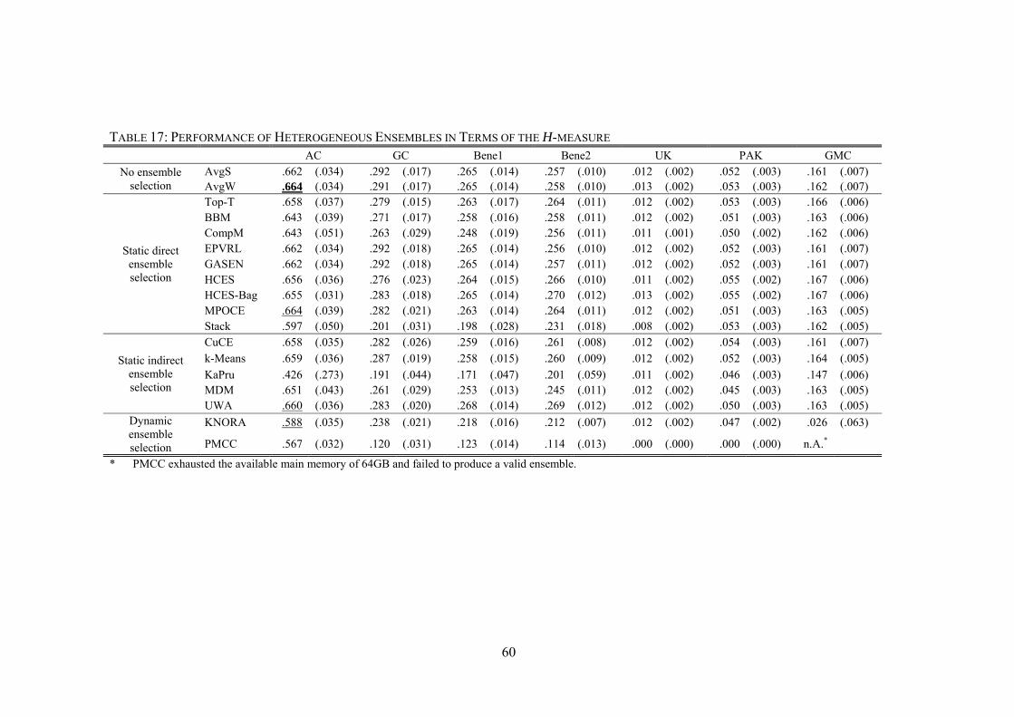
60
TABLE 17: PERFORMANCE OF HETEROGENEOUS ENSEMBLES IN TERMS OF THE H-MEASURE AC GC Bene1 Bene2 UK PAK GMC
No ensemble selection
AvgS .662 (.034) .292 (.017) .265 (.014) .257 (.010) .012 (.002) .052 (.003) .161 (.007) AvgW .664 (.034) .291 (.017) .265 (.014) .258 (.010) .013 (.002) .053 (.003) .162 (.007)
Static direct ensemble selection
Top-T .658 (.037) .279 (.015) .263 (.017) .264 (.011) .012 (.002) .053 (.003) .166 (.006) BBM .643 (.039) .271 (.017) .258 (.016) .258 (.011) .012 (.002) .051 (.003) .163 (.006) CompM .643 (.051) .263 (.029) .248 (.019) .256 (.011) .011 (.001) .050 (.002) .162 (.006) EPVRL .662 (.034) .292 (.018) .265 (.014) .256 (.010) .012 (.002) .052 (.003) .161 (.007) GASEN .662 (.034) .292 (.018) .265 (.014) .257 (.011) .012 (.002) .052 (.003) .161 (.007) HCES .656 (.036) .276 (.023) .264 (.015) .266 (.010) .011 (.002) .055 (.002) .167 (.006) HCES-Bag .655 (.031) .283 (.018) .265 (.014) .270 (.012) .013 (.002) .055 (.002) .167 (.006) MPOCE .664 (.039) .282 (.021) .263 (.014) .264 (.011) .012 (.002) .051 (.003) .163 (.005) Stack .597 (.050) .201 (.031) .198 (.028) .231 (.018) .008 (.002) .053 (.003) .162 (.005)
Static indirect ensemble selection
CuCE .658 (.035) .282 (.026) .259 (.016) .261 (.008) .012 (.002) .054 (.003) .161 (.007) k-Means .659 (.036) .287 (.019) .258 (.015) .260 (.009) .012 (.002) .052 (.003) .164 (.005)
KaPru .426 (.273) .191 (.044) .171 (.047) .201 (.059) .011 (.002) .046 (.003) .147 (.006) MDM .651 (.043) .261 (.029) .253 (.013) .245 (.011) .012 (.002) .045 (.003) .163 (.005) UWA .660 (.036) .283 (.020) .268 (.014) .269 (.012) .012 (.002) .050 (.003) .163 (.005)
Dynamic ensemble selection
KNORA .588 (.035) .238 (.021) .218 (.016) .212 (.007) .012 (.002) .047 (.002) .026 (.063)
PMCC .567 (.032) .120 (.031) .123 (.014) .114 (.013) .000 (.000) .000 (.000) n.A.*
* PMCC exhausted the available main memory of 64GB and failed to produce a valid ensemble.