Benchmarking of Unconditional VaR and ES Calculation Methods: A Comparative Simulation Analysis with Truncated Stable Distribution Takashi Isogai * takashi.isogai@boj.or.jp

No.14-E-1 January 2014

Bank of Japan 2-1-1 Nihonbashi-Hongokucho, Chuo-ku, Tokyo 103-0021, Japan

* Financial System and Bank Examination Department

Papers in the Bank of Japan Working Paper Series are circulated in order to stimulate discussion and comments. Views expressed are those of authors and do not necessarily reflect those of the Bank. If you have any comment or question on the working paper series, please contact each author.

When making a copy or reproduction of the content for commercial purposes, please contact the Public Relations Department (post.prd8@boj.or.jp) at the Bank in advance to request permission. When making a copy or reproduction, the source, Bank of Japan Working Paper Series, should explicitly be credited.

Bank of Japan Working Paper Series

This page intentionally left blank.

1

Benchmarking of Unconditional VaR and ES Calculation Methods: A Comparative Simulation Analysis with Truncated Stable Distribution*

Takashi Isogai†

January 2014

Abstract

This paper analyzes Value at Risk (VaR) and Expected Shortfall (ES) calculation methods in terms of

bias and dispersion against benchmarks computed from a fat-tailed parametric distribution. The daily log

returns of the Nikkei-225 stock index are modeled by a truncated stable distribution. The VaR and ES

values of the fitted distribution are regarded as benchmarks. The fitted distribution is also used as a

sampling distribution; sample returns with different sizes are generated for the simulations of the VaR and

ES calculations. Two parametric methods: normal distribution and generalized Pareto distribution and

two non-parametric methods: historical simulation and kernel smoothing are selected as the targets of this

analysis. A comparison of the simulated VaR, ES, and the ES/VaR ratio with the benchmarks at multiple

confidence levels reveals that the normal distribution approximation has a significant downward bias,

especially in the ES calculation. The estimates by the other three methods are much closer to the

benchmarks on average, although some of them become unstable with smaller sample sizes and/or at

higher confidence levels. Specifically, ES tends to be more biased and unstable than VaR at higher

confidence levels.

Keywords: Value at Risk, Expected Shortfall, Fat-Tailed Distribution, Truncated Stable Distribution,

Numerical Simulation.

* The views and opinions expressed here are solely those of the author and do not necessarily represent or reflect those of, nor should be attributed to Bank of Japan. † Financial System and Bank Examination Department, Bank of Japan. Email: takashi.isogai@boj.or.jp.

2

Table of contents

1 Introduction ........................................................................................................................................... 3

2 Framework of comparative analysis of the VaR and ES calculation .................................................... 3

2.1 Modeling asset return and risk measurement ................................................................................ 3

2.2 Numerical simulation based on random sampling ......................................................................... 4

2.3 Truncated stable distribution as population distribution ................................................................ 6

3 Parameter estimates and numerical simulation for benchmarking........................................................ 9

3.1 Parameter estimate of truncated stable distribution ....................................................................... 9

3.2 VaR and ES of truncated stable distribution as benchmarks ....................................................... 12

3.3 Random sampling with stress losses ............................................................................................ 15

3.4 Details of calculation methods and simulation settings ............................................................... 17

4 Simulation results and evaluation ....................................................................................................... 26

4.1 Bias and precision of VaR and ES ............................................................................................... 27

4.2 Relative performance ................................................................................................................... 35

4.3 The ES/VaR ratio ......................................................................................................................... 39

5 Concluding remarks ............................................................................................................................ 40

References ................................................................................................................................................... 44

3

1 Introduction

Expected Shortfall (ES) estimates are garnering growing interest as an alternative risk measure of asset returns replacing VaR, since the weakness of the latter, especially its inability to capture tail risks, was widely recognized after the Lehman shock. The Basel Committee on Banking Supervision proposed the use of ES for calculating the required level of capital in trading accounts. This paper studies the bias and dispersion of the VaR and ES calculation methods by numerical simulations with data sampled from a fitted fat-tailed distribution. The accuracy of the risk measures is analyzed based on the comparison with the benchmarks at multiple confidence levels. This approach is fundamentally different from the back-testing1 approach for model validation, which is regularly used by financial institutions. It would be useful to combine these two techniques as supplementary tools to detect hidden model risks. It should be mentioned that the analysis in this study is limited to the case of a single asset return; therefore, the correlation of asset returns and risk aggregation are out of the scope of this research.2 The advantages and disadvantages of the VaR and ES approaches from a theoretical viewpoint are not discussed either.

This paper is organized as follows. Section 2 describes the framework of the VaR and ES analysis based on the benchmark approach. Section 3 deals with the selection of a sampling distribution and fitting the distribution to the Nikkei-225 stock index (the Nikkei). This section also contains the details of VaR and ES calculation methods as well as the settings for data sampling for the numerical simulation. Section 4 evaluates the accuracy and precision3 of the VaR and ES estimates by the four methods. Section 5 contains the conclusions and discusses some open issues that may be explored in future research.

2 Framework of comparative analysis of the VaR and ES calculation

2.1 Modeling asset return and risk measurement

2.1.1 Risk measures

VaR is the maximum loss of an investment at a certain confidence level over a specified time horizon; ES is the mean of the losses, given that losses are greater than those under VaR at the same confidence level. VaR and ES are defined as follows, where X is an asset return and p is the confidence level:4

[ ] [ ]{ } 10,1|inf <<−>≤−= ppxXPxXVaRp

[ ] [ ][ ] 10,| <<≥−−= pXVaRXXEXES pp

(1)

1 Back testing is a technique used to reconcile forecasted losses from VaR or ES with actual losses at the end of the time horizon. 2 Yoshiba (2013) studies risk aggregation by various copula under stressed conditions. 3 Bias is the average difference between the estimator and the true value. The estimator of the risk measure is more accurate when it is less biased. Precision is often defined as the standard deviation of the estimator. It is important to examine both accuracy and precision for validating a calculation method of a risk measure. 4 In this paper, both VaR and ES are measured as positive numbers in terms of log return.

4

ES is believed to fulfill many requirements of a good risk measure; for example, it is a coherent risk measure (Artzner et al. (1999)),5 while VaR is not, as it does not satisfy the sub-additivity property. More importantly, from a viewpoint of capturing tail risk, ES considers losses beyond the VaR level, while VaR disregards losses beyond the percentile, as mentioned by the Basel Committee in their initial proposals6 with regard to the trading book capital requirement policies.

2.1.2 Modeling asset returns and risk measurement

The first step to calculate VaR and ES is to model an asset return by some conditional or unconditional probabilistic distribution. The unconditional model assumes that the distribution of the asset return is stationary and not affected by time shift, while the conditional model depends on the history of risk factors such as volatility. The two approaches are fundamentally different in that the conditional model captures the changes over time whereas the unconditional one does not. For example, volatility is a conditional factor when the asset return is calculated by a GARCH model, in which the phenomenon of so-called volatility clustering is well captured. It is crucial to clarify which method is employed, since the estimates of VaR and ES are largely dependent on this. It is not necessarily clear which method should be used for risk measurement, since many factors need to be considered. The purpose of risk measurement may be of some help in this regard; the unconditional model is easy to implement in stress testing and capital planning that requires complicated risk aggregation from desk levels, while the conditional model is useful for more responsive risk measurement.7 This paper focuses on the unconditional VaR and ES calculations;8 therefore, the unconditional model approach is adopted.

Under the unconditional approach, it is most important to find a distribution that best matches the fat-tailness observed in actual returns, as an inadequate choice may cause serious problems, including the underestimation of risk.

2.2 Numerical simulation based on random sampling

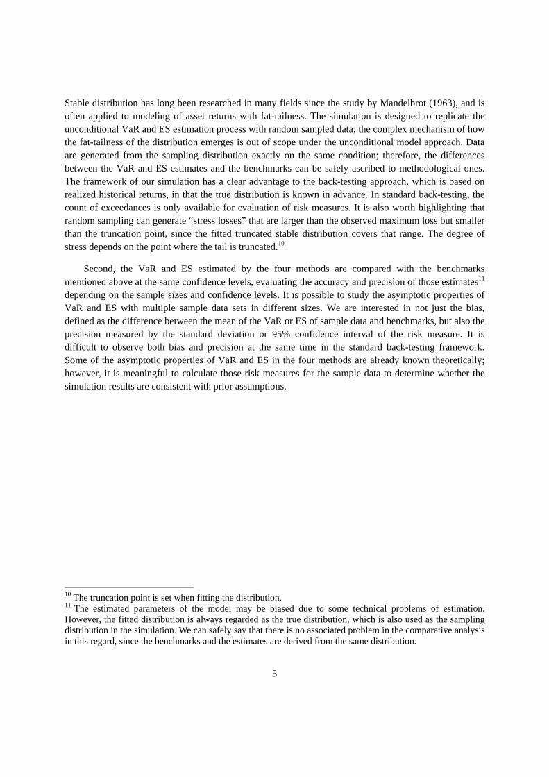
Figure 1 illustrates the overall framework of the simulation. First, the selected fat-tailed distribution is fitted to the log returns of the Nikkei in order to calculate the benchmarks of VaR and ES of the distribution as well as to generate data by random sampling for the simulation of VaR and ES estimates. We have chosen a truncated stable distribution,9 the tail of which is bounded both below and above.

5 A coherent risk measure satisfies the properties of monotonicity, sub-additivity, positive homogeneity, and translational invariance. 6 Basel Committee on Banking Supervision (2012). 7 According to McNeil and Frey (2000) and Alexander and Sheedy (2008), more accurate VaR estimates are available using conditional VaR models for financial assets like stocks and exchange rates. 8 Many Japanese financial institutions including regional banks seem to adopt the unconditional approach in implementing VaR calculation methods such as variance-covariance and historical simulation. Alexander and Ledermann (2012) stated that major banks still base VaR estimates on unconditional distributions for risk factor returns. They analyzed the reasons as follows: the conditional VaR models are far too complex, econometrically and computationally, to be integrated into an enterprise-wide risk assessment framework, and the market risk capital allocations that are derived from them would change too much over time. 9 Stable distribution is also called the α-stable distribution, the Lévy alpha stable, and the Pareto Lévy stable distribution.

5

Stable distribution has long been researched in many fields since the study by Mandelbrot (1963), and is often applied to modeling of asset returns with fat-tailness. The simulation is designed to replicate the unconditional VaR and ES estimation process with random sampled data; the complex mechanism of how the fat-tailness of the distribution emerges is out of scope under the unconditional model approach. Data are generated from the sampling distribution exactly on the same condition; therefore, the differences between the VaR and ES estimates and the benchmarks can be safely ascribed to methodological ones. The framework of our simulation has a clear advantage to the back-testing approach, which is based on realized historical returns, in that the true distribution is known in advance. In standard back-testing, the count of exceedances is only available for evaluation of risk measures. It is also worth highlighting that random sampling can generate “stress losses” that are larger than the observed maximum loss but smaller than the truncation point, since the fitted truncated stable distribution covers that range. The degree of stress depends on the point where the tail is truncated.10

Second, the VaR and ES estimated by the four methods are compared with the benchmarks mentioned above at the same confidence levels, evaluating the accuracy and precision of those estimates11 depending on the sample sizes and confidence levels. It is possible to study the asymptotic properties of VaR and ES with multiple sample data sets in different sizes. We are interested in not just the bias, defined as the difference between the mean of the VaR or ES of sample data and benchmarks, but also the precision measured by the standard deviation or 95% confidence interval of the risk measure. It is difficult to observe both bias and precision at the same time in the standard back-testing framework. Some of the asymptotic properties of VaR and ES in the four methods are already known theoretically; however, it is meaningful to calculate those risk measures for the sample data to determine whether the simulation results are consistent with prior assumptions.

10 The truncation point is set when fitting the distribution. 11 The estimated parameters of the model may be biased due to some technical problems of estimation. However, the fitted distribution is always regarded as the true distribution, which is also used as the sampling distribution in the simulation. We can safely say that there is no associated problem in the comparative analysis in this regard, since the benchmarks and the estimates are derived from the same distribution.

6

Figure 1. Framework of numerical simulation

The following sub-sections describe the details of the simulation and comparative analyses as well as the settings for the individual VaR and ES estimation methods.

2.3 Truncated stable distribution as population distribution

2.3.1 Modeling asset returns by stable distribution

While financial theories and applications frequently assume that asset returns are normally distributed, substantial empirical data contradict this assumption. The unconditional model assumes that asset returns are independent and identically distributed (i.i.d.) and hence the distribution of the sum of variables, each with a finite variance, converges to normal as the number of variables increases, even when each distribution is non-normal (the central limit theorem, CLT). The CLT is not, however, valid without the finite variance assumption; the limit would then be a stable distribution (Generalized CLT, GCLT). The normal distribution is one family of stable distributions with some specific values of distributional parameters. Stable distribution has some convenient features in that it can well model asset returns with greater flexibility replicating fatter tails and/or asymmetry observed. Stable distribution is also useful for time scaling of asset returns.

population distribution: truncated stable

Nikkei, log returns

fitting

VaR, ES as bencmarks

random sampling

sample data set: 1000 sets of 250 ～ 1000 sample sizes

comparison of bias and stability

VaR, ES,VaR/ES

・confidence level by sample size per a data set

Four methods of unconditional VaR and ES calculation

Normal GPD Historical simulation Kernel smoothing

VaR, ES,VaR/ES

VaR, ES,VaR/ES

VaR, ES,VaR/ES

7

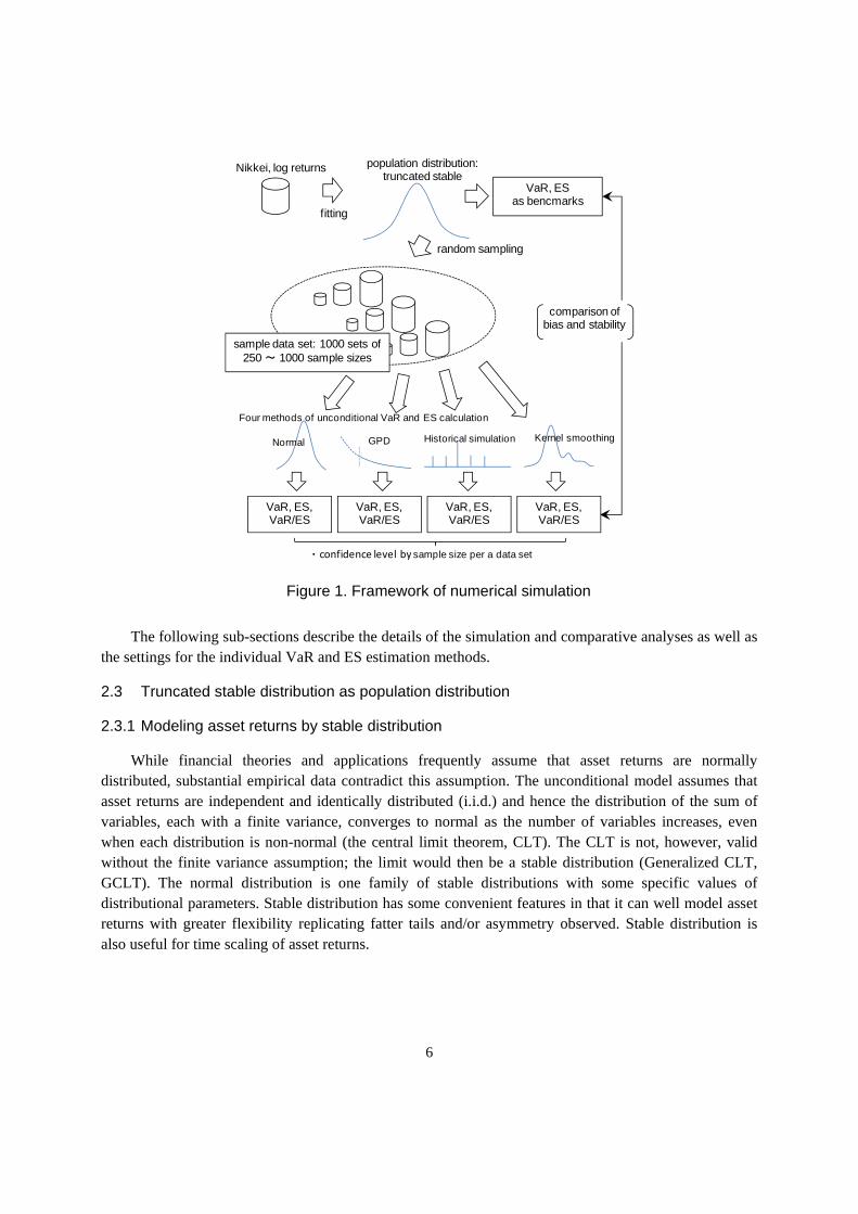
2.3.2 Properties of stable distribution

A random variable X is stable if and only if there are constants ( )0>NN CC and ND for all N > 1

such that:

NN

d

NNN DXCSXXXS +=+++= ,21 L (2)12

where NS is the sum of NXX ,,1L : independent copies of random variables X. When X is an asset

return, the distribution remains the same stable distribution13 even after time scaling of the return from

daily X to monthly NS , although the location and scale of the scaled distribution are changed.

The distribution of a stable random variable X is defined through its characteristic function, since a closed from of the density function of the stable distribution is not available except for some special cases mentioned later. The characteristic function can be equivalently converted to a probability density

function (PDF) or a cumulative distribution function (CDF). The PDF of the stable distribution)(xf is

provided as the inverse Fourier transform of the characteristic function as below:

( ) ( )∫∞

∞−−= duuCiuxxf Xexp

2

1)(

π (3)

where ( ) [ ])exp(iuXEuCX = is the characteristic function of the stable distribution. The characteristic

function ( )uCX is given by14

( )( )( )

( )( ) ( )( )

>=<−

=

=

+

+−

≠

+

−

+−=

−

0,1

0,0

0,1

sign

1,logsign2

1exp

1,1sign2

tan1exp1

u

u

u

u

uiuuiu

uiuuiu

uCX

αδγπ

βγ

αδγπαβγ ααα

(4)

A general stable distribution has four parameters: the index of stability α, also called the tail index, the skewness parameter β, the scale parameter γ, and the location parameter δ. The range of parameter α, β, and γ must satisfy the following conditions respectively:

0,11,20 ≥≤≤−≤< γβα (5)

The two parameters α and β play a key role in determining the shape of the stable distribution. Specifically, the stability index α determines the rate at which the tails of the distribution taper off. The

12 The notation d

= denotes equality in distribution. 13 The term stable distribution reflects the fact that the sum of i.i.d. random variables having a stable distribution with the same index α is again stable with the same value of α. 14 There are multiple styles of parameterizations of a stable distribution. The definition of the parameter α is the same in any parameterization style; however, the other three parameters can be denoted differently depending on the style. For more details of the parameterization, see Nolan (2013) and Misiorek and Rafael (2012).

8

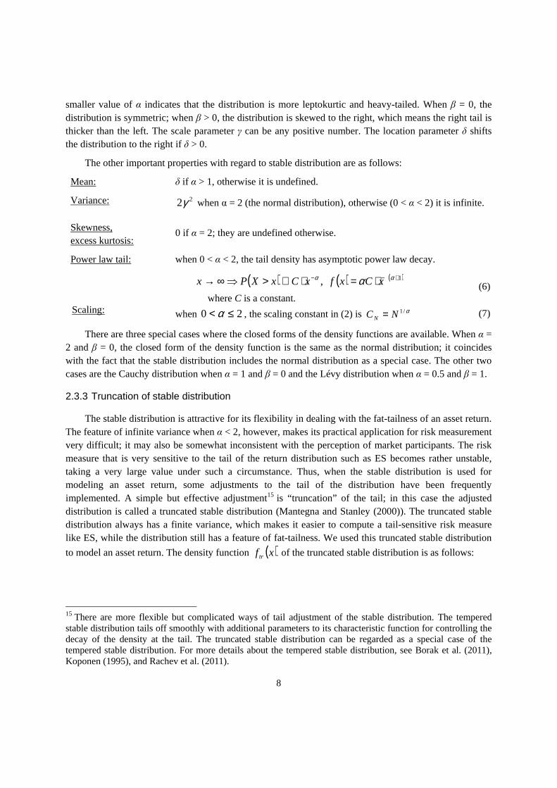
smaller value of α indicates that the distribution is more leptokurtic and heavy-tailed. When β = 0, the distribution is symmetric; when β > 0, the distribution is skewed to the right, which means the right tail is thicker than the left. The scale parameter γ can be any positive number. The location parameter δ shifts the distribution to the right if δ > 0.

The other important properties with regard to stable distribution are as follows:

Mean: δ if α > 1, otherwise it is undefined.

Variance: 22γ when α = 2 (the normal distribution), otherwise (0 < α < 2) it is infinite.

Skewness, excess kurtosis:

0 if α = 2; they are undefined otherwise.

Power law tail: when 0 < α < 2, the tail density has asymptotic power law decay.

( ) ( ) ( )1, +−− ⋅=⋅∝>⇒∞→ αα α xCxfxCxXPx

where C is a constant. (6)

Scaling: when 20 ≤< α , the scaling constant in (2) is α/1NCN = (7)

There are three special cases where the closed forms of the density functions are available. When α = 2 and β = 0, the closed form of the density function is the same as the normal distribution; it coincides with the fact that the stable distribution includes the normal distribution as a special case. The other two cases are the Cauchy distribution when α = 1 and β = 0 and the Lévy distribution when α = 0.5 and β = 1.

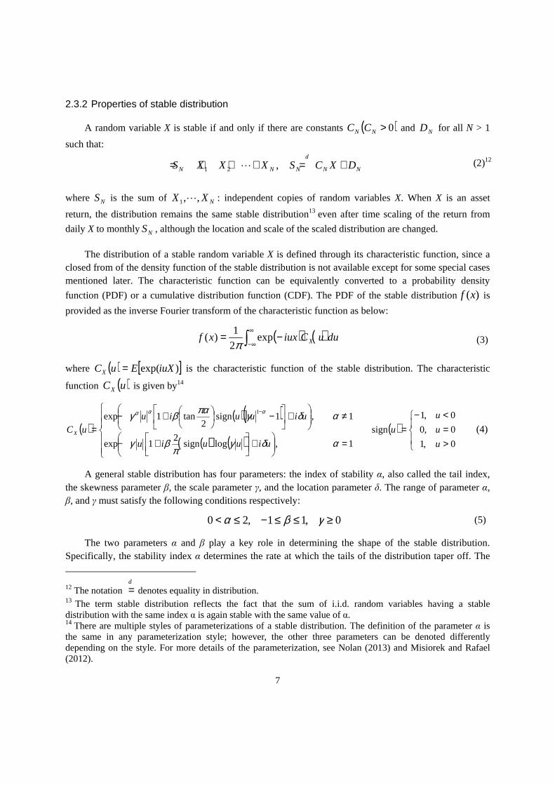
2.3.3 Truncation of stable distribution

The stable distribution is attractive for its flexibility in dealing with the fat-tailness of an asset return. The feature of infinite variance when α < 2, however, makes its practical application for risk measurement very difficult; it may also be somewhat inconsistent with the perception of market participants. The risk measure that is very sensitive to the tail of the return distribution such as ES becomes rather unstable, taking a very large value under such a circumstance. Thus, when the stable distribution is used for modeling an asset return, some adjustments to the tail of the distribution have been frequently implemented. A simple but effective adjustment15 is “truncation” of the tail; in this case the adjusted distribution is called a truncated stable distribution (Mantegna and Stanley (2000)). The truncated stable distribution always has a finite variance, which makes it easier to compute a tail-sensitive risk measure like ES, while the distribution still has a feature of fat-tailness. We used this truncated stable distribution

to model an asset return. The density function ( )xftr of the truncated stable distribution is as follows:

15 There are more flexible but complicated ways of tail adjustment of the stable distribution. The tempered stable distribution tails off smoothly with additional parameters to its characteristic function for controlling the decay of the density at the tail. The truncated stable distribution can be regarded as a special case of the tempered stable distribution. For more details about the tempered stable distribution, see Borak et al. (2011), Koponen (1995), and Rachev et al. (2011).

9

( ) ( )

<≤≤⋅

>=

a

bal

b

tr

lx

lxlxfc

lx

xf

,0

,

,0

( 0,0 >< ba ll )

( )xf is the density function of the stable distribution as in (3); lc is a constant

that satisfies ( ) 1=⋅∫ dxxfcb

a

l

l l ; if ba ll −= , the truncation is symmetrical.

(8)

The parameters of the truncated stable distribution can be estimated by MLE with numerical optimization; the truncation points are a pair of constant values, which can be inferred from the properties of the financial asset or some market safety function like a circuit breaker, if any.16 If not a circuit breaker or a similar function, the truncation points can be set at any points beyond the observed maximum loss (or gain) without upper limits; any levels selected seem to be arbitrary. The problem is that the selection of the truncation points can directly affect the level of the risk measure. Specifically, ES of the truncated stable distribution is largely dependent on the truncation points.17 Random sampling from the truncated stable distribution and benchmarking of VaR and ES in our simulation are still valid as long as the parameters of the truncated stable distribution are fixed. The problem, however, would be crucial when using the truncated stable distribution for the VaR and ES calculation.

3 Parameter estimates and numerical simulation for benchmarking

3.1 Parameter estimate of truncated stable distribution

The parameters of the sampling distribution should be realistic in order to make the simulation analysis meaningful. In this respect, we have selected the Nikkei as a typical financial asset for modeling by the truncated stable distribution. Figure 2 shows the daily log return18 of the Nikkei from January 2008 to August 2012. Significant changes in volatility have been observed during the Lehman shock in 2008 and the Great East Japan Earthquake in 2012. In Figure 3, the estimated density by kernel smoothing (the left pane) indicates that the return distribution seems to be more leptokurtic and heavy-tailed than the normal distribution. The QQ plot (the right pane) also reveals that the distribution is significantly fat-tailed. The results of several normality tests (Table 1) also show that the distribution is far from the normal distribution.

16 For example, a single-stock circuit breaker is triggered after a trade occurs at or outside of the applicable percentage thresholds; trading is halted thereafter. Truncating the distribution at levels that correspond to the thresholds will result in zero probability of over-the-limit prices. 17 The degree of impact on VaR and ES by truncation of stable distribution is calculated and summarized in Table 6. 18 A financial asset return is often measured in terms of logarithmic return. We also use the log return scale for risk quantification here.

10

Figure 2. Performance and log returns of the Nikkei

Figure 3. Density function and QQ plot of the Nikkei

8000

10000

12000

14000

Nikkei

year

2008 2009 2010 2011 2012

-0.1

0-0

.05

0.00

0.05

0.10

Nikkei(log return)

year

2008 2009 2010 2011 2012

Histgram(left), density(right)

-0.15 -0.10 -0.05 0.00 0.05 0.10 0.15

0

100

200

300

400

0

5

10

15

20

25

30EmpiricalNormal

-0.06 -0.04 -0.02 0.00 0.02 0.04 0.06

-0.1

0-0

.05

0.00

0.05

0.10

QQ-plot

Normal

data

11

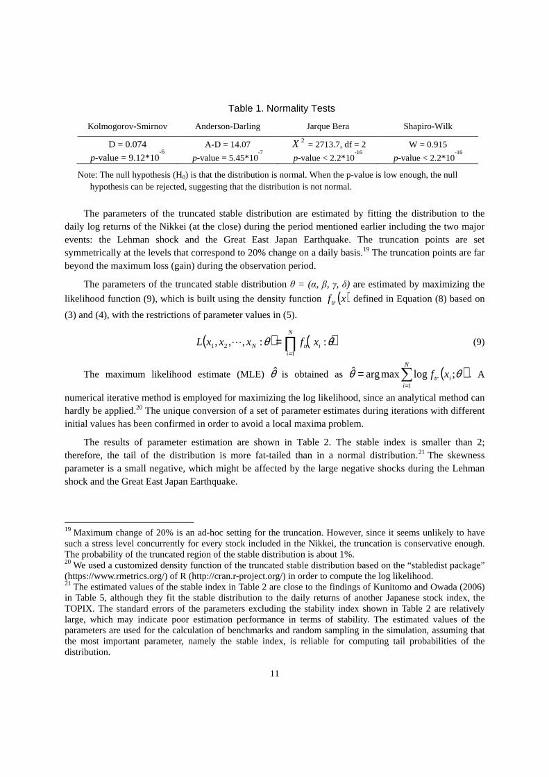
Table 1. Normality Tests

Kolmogorov-Smirnov Anderson-Darling Jarque Bera Shapiro-Wilk

D = 0.074

p-value = 9.12*10-6

A-D = 14.07

p-value = 5.45*10-7

2X = 2713.7, df = 2

p-value < 2.2*10-16

W = 0.915

p-value < 2.2*10-16

Note: The null hypothesis (H0) is that the distribution is normal. When the p-value is low enough, the null hypothesis can be rejected, suggesting that the distribution is not normal.

The parameters of the truncated stable distribution are estimated by fitting the distribution to the daily log returns of the Nikkei (at the close) during the period mentioned earlier including the two major events: the Lehman shock and the Great East Japan Earthquake. The truncation points are set symmetrically at the levels that correspond to 20% change on a daily basis.19 The truncation points are far beyond the maximum loss (gain) during the observation period.

The parameters of the truncated stable distribution θ = (α, β, γ, δ) are estimated by maximizing the

likelihood function (9), which is built using the density function ( )xftr defined in Equation (8) based on

(3) and (4), with the restrictions of parameter values in (5).

( ) ( )∏=

=N

iitrN xfxxxL

121 ::,,, θθL (9)

The maximum likelihood estimate (MLE) θ̂ is obtained as ( )∑=

=N

iitr xf

1

;logmaxargˆ θθ . A

numerical iterative method is employed for maximizing the log likelihood, since an analytical method can hardly be applied.20 The unique conversion of a set of parameter estimates during iterations with different initial values has been confirmed in order to avoid a local maxima problem.

The results of parameter estimation are shown in Table 2. The stable index is smaller than 2; therefore, the tail of the distribution is more fat-tailed than in a normal distribution.21 The skewness parameter is a small negative, which might be affected by the large negative shocks during the Lehman shock and the Great East Japan Earthquake.

19 Maximum change of 20% is an ad-hoc setting for the truncation. However, since it seems unlikely to have such a stress level concurrently for every stock included in the Nikkei, the truncation is conservative enough. The probability of the truncated region of the stable distribution is about 1%. 20 We used a customized density function of the truncated stable distribution based on the “stabledist package” (https://www.rmetrics.org/) of R (http://cran.r-project.org/) in order to compute the log likelihood. 21 The estimated values of the stable index in Table 2 are close to the findings of Kunitomo and Owada (2006) in Table 5, although they fit the stable distribution to the daily returns of another Japanese stock index, the TOPIX. The standard errors of the parameters excluding the stability index shown in Table 2 are relatively large, which may indicate poor estimation performance in terms of stability. The estimated values of the parameters are used for the calculation of benchmarks and random sampling in the simulation, assuming that the most important parameter, namely the stable index, is reliable for computing tail probabilities of the distribution.

12

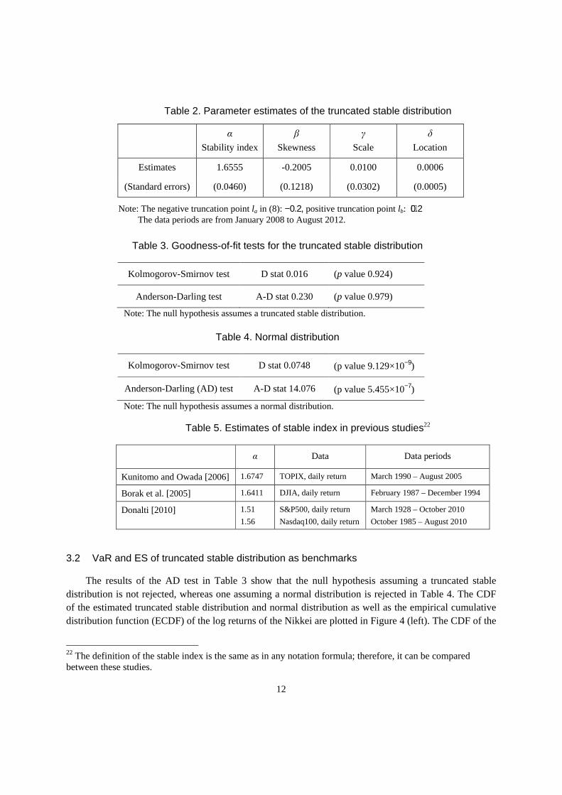
Table 2. Parameter estimates of the truncated stable distribution

α Stability index

β Skewness

γ Scale

δ Location

Estimates 1.6555 -0.2005 0.0100 0.0006

(Standard errors) (0.0460) (0.1218) (0.0302) (0.0005)

Note: The negative truncation point la in (8): −0.2, positive truncation point lb: +0.2 The data periods are from January 2008 to August 2012.

Table 3. Goodness-of-fit tests for the truncated stable distribution

Kolmogorov-Smirnov test D stat 0.016 (p value 0.924)

Anderson-Darling test A-D stat 0.230 (p value 0.979)

Note: The null hypothesis assumes a truncated stable distribution.

Table 4. Normal distribution

Kolmogorov-Smirnov test D stat 0.0748 (p value 9.129×10−9)

Anderson-Darling (AD) test A-D stat 14.076 (p value 5.455×10−7)

Note: The null hypothesis assumes a normal distribution.

Table 5. Estimates of stable index in previous studies22

α Data Data periods

Kunitomo and Owada [2006] 1.6747 TOPIX, daily return March 1990 – August 2005

Borak et al. [2005] 1.6411 DJIA, daily return February 1987 – December 1994

Donalti [2010] 1.51

1.56

S&P500, daily return

Nasdaq100, daily return

March 1928 – October 2010

October 1985 – August 2010

3.2 VaR and ES of truncated stable distribution as benchmarks

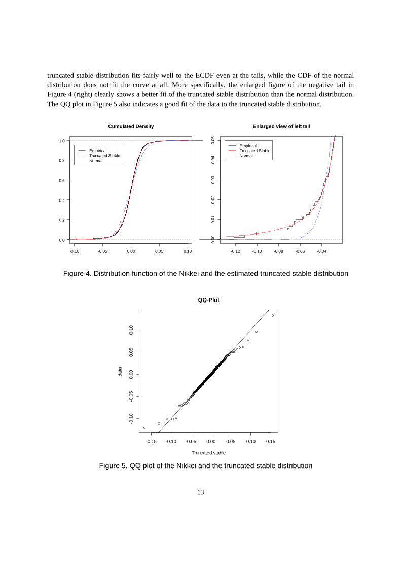
The results of the AD test in Table 3 show that the null hypothesis assuming a truncated stable distribution is not rejected, whereas one assuming a normal distribution is rejected in Table 4. The CDF of the estimated truncated stable distribution and normal distribution as well as the empirical cumulative distribution function (ECDF) of the log returns of the Nikkei are plotted in Figure 4 (left). The CDF of the

22 The definition of the stable index is the same as in any notation formula; therefore, it can be compared between these studies.

13

truncated stable distribution fits fairly well to the ECDF even at the tails, while the CDF of the normal distribution does not fit the curve at all. More specifically, the enlarged figure of the negative tail in Figure 4 (right) clearly shows a better fit of the truncated stable distribution than the normal distribution. The QQ plot in Figure 5 also indicates a good fit of the data to the truncated stable distribution.

Figure 4. Distribution function of the Nikkei and the estimated truncated stable distribution

Figure 5. QQ plot of the Nikkei and the truncated stable distribution

-0.10 -0.05 0.00 0.05 0.10

0.0

0.2

0.4

0.6

0.8

1.0

Cumulated Density

EmpiricalTruncated StableNormal

-0.12 -0.10 -0.08 -0.06 -0.04

0.00

0.01

0.02

0.03

0.04

0.05

Enlarged view of left tail

EmpiricalTruncated StableNormal

-0.15 -0.10 -0.05 0.00 0.05 0.10 0.15

-0.1

0-0

.05

0.00

0.05

0.10

QQ-Plot

Truncated stable

data

14

Both VaR and ES of the truncated stable distribution, which serve as the benchmarks in our comparative analysis, are computed by a numerical calculation method using the density function (8) and the definition of VaR and ES (1), since it is very difficult to derive their analytical forms. The confidence levels of VaR and ES are set at each percentage point from 95% to 99%; three more points at 99.5%, 99.7%, and 99.9% at the extreme tail. The calculated VaR and ES as well as the ES/VaR ratio are plotted in Figure 6.

Figure 6. VaR, ES, and the ES/VaR ratio as benchmarks of the truncated stable distribution

ES is always larger than VaR at the same confidence level by definition (1) as shown in Figure 6 (left). Both VaR and ES increase as the confidence level rises; the pace of this increase accelerates at confidence levels higher than 99%. On the contrary, the ES/VaR ratio, which captures the degree of tail risk that is not captured by VaR, decreases as the confidence level rises in Figure 6 (right). The ratio approaches 1, the theoretical convergence level assuming finite variance of the distribution. It is apparent that ES better captures tail risks as compared to VaR; however, the distance between ES and VaR becomes smaller at confidence levels of over 99% as shown in Figure 6 (left). The ES/VaR ratio also decreases much faster at those high confidence levels. These observations mean that ES provides only limited additional information with regard to the tail risks at extremely high confidence levels.

An important caveat should be mentioned with regard to the use of the truncated stable distribution. When modeling an asset return by such a distribution, measured risk, especially in terms of ES, is largely dependent on truncation points: the longer the tails of the distribution, the larger the ES. In many cases, we need to truncate the distribution at arbitrary locations without any objective criteria assuming possible stress losses. Table 6 summarizes the degree of impact on VaR and ES by truncation of stable distribution. It shows that the lower the truncation points or the higher the confidence level, the larger the decrease of the VaR and ES, showing the smaller numbers in the table. It confirms that the impact of truncation is

95 96 97 98 99 100

0.04

0.06

0.08

0.10

0.12

0.14

0.16

VaR, ES of truncated stable

confidence level

95 96 97 98 99 100

0.04

0.06

0.08

0.10

0.12

0.14

0.16

VaRES

95 96 97 98 99 100

1.2

1.3

1.4

1.5

1.6

1.7

ES/VaR of truncated stable

confidence level

15

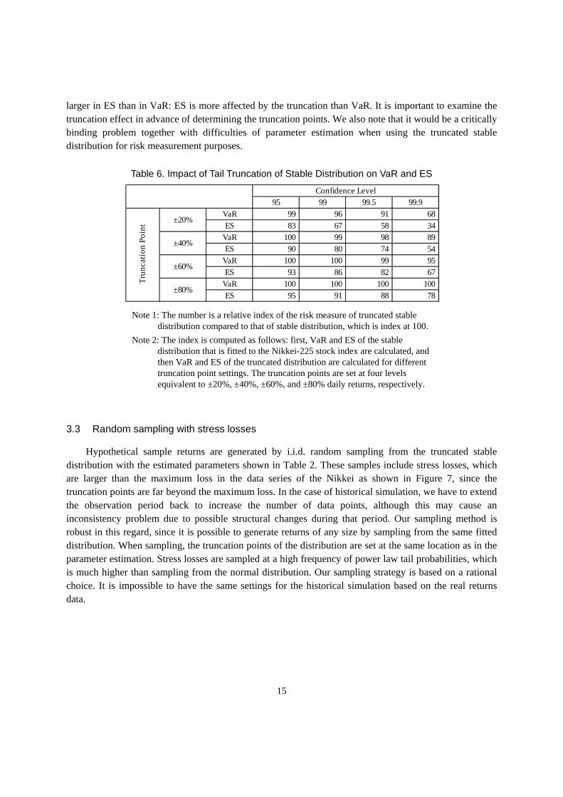
larger in ES than in VaR: ES is more affected by the truncation than VaR. It is important to examine the truncation effect in advance of determining the truncation points. We also note that it would be a critically binding problem together with difficulties of parameter estimation when using the truncated stable distribution for risk measurement purposes.

Table 6. Impact of Tail Truncation of Stable Distribution on VaR and ES

Note 1: The number is a relative index of the risk measure of truncated stable distribution compared to that of stable distribution, which is index at 100.

Note 2: The index is computed as follows: first, VaR and ES of the stable distribution that is fitted to the Nikkei-225 stock index are calculated, and then VaR and ES of the truncated distribution are calculated for different truncation point settings. The truncation points are set at four levels equivalent to ±20%, ±40%, ±60%, and ±80% daily returns, respectively.

3.3 Random sampling with stress losses

Hypothetical sample returns are generated by i.i.d. random sampling from the truncated stable distribution with the estimated parameters shown in Table 2. These samples include stress losses, which are larger than the maximum loss in the data series of the Nikkei as shown in Figure 7, since the truncation points are far beyond the maximum loss. In the case of historical simulation, we have to extend the observation period back to increase the number of data points, although this may cause an inconsistency problem due to possible structural changes during that period. Our sampling method is robust in this regard, since it is possible to generate returns of any size by sampling from the same fitted distribution. When sampling, the truncation points of the distribution are set at the same location as in the parameter estimation. Stress losses are sampled at a high frequency of power law tail probabilities, which is much higher than sampling from the normal distribution. Our sampling strategy is based on a rational choice. It is impossible to have the same settings for the historical simulation based on the real returns data.

95 99 99.5 99.9VaR 99 96 91 68ES 83 67 58 34

VaR 100 99 98 89ES 90 80 74 54

VaR 100 100 99 95ES 93 86 82 67

VaR 100 100 100 100ES 95 91 88 78

Confidence Level

Tru

nca

tio

n P

oin

t ±20%

±40%

±60%

±80%

16

Figure 7. Random sampling from the fitted truncated stable distribution

One thousand sets of samples with different sizes: n = 250, 500, 1000, and 2000 were generated from the fitted truncated stable distribution by rejection sampling. The smallest size of 250 is approximately the number of trading days in a year. The larger sample sets correspond to longer trading days.

The i.i.d. random samples are completely different from the actual time series of returns. The actual returns show volatility clustering, which is a typical feature of financial return series, as shown in Figure 2 (right). The unconditional model is a static model that disregards inter-temporal effects on returns. Figure 8 (left) shows a random permutation of the Nikkei returns, which has lost the inter-temporal feature of a financial return; therefore can be comparable to the i.i.d. random samples in Figure 8 (right). Thus, we use random samples for the simulation, since the unconditional model actually assumes this type of randomized data. Such randomized data satisfy the stationarity condition, which is implicitly assumed in the unconditional model.

range of observed data

range of truncated stable distribution

maximum loss

truncationpoint

Density of truncated stable distribution

Stressed loss larger than maximum loss

Density

return

Density of normal distribution

sample data

17

Figure 8. Random permutation of the Nikkei and the random samples in equal size

3.4 Details of calculation methods and simulation settings

Two parametric23 methods assuming normal distribution and generalized Pareto distribution (GPD), and two non-parametric methods, namely, historical simulation and kernel smoothing are selected as the targets of analysis. These methods are widely used for risk measurement by financial institutions. As for confidence levels, the same settings as in the calculation of VaR and ES benchmarks were adopted, i.e., at the range of 95% to 99% increasing by one percentage point and at 99.5%, 99.7%, and 99.9%.

First, VaR and ES for every random sample set are calculated by the above-mentioned four methods at all confidence levels. Then, the averages of VaR and ES are calculated respectively over 1000 sets with the same sample size at all confidence levels, which are compared to the benchmarks for detecting biases. The benchmarks are calculated directly using the density function (8) of the fitted distribution at the same confidence levels. The 95% confidence intervals24 as well as the standard deviations from the average are calculated at every confidence level to evaluate how the precision of those estimates is affected by the sample sizes and confidence levels.25 The following sections delve into the technical details and the parameter configurations for each calculation method of VaR and ES.

23 In this paper, a parametric method is defined one in which distributional parameters are inferred to quantify the risk measures, whereas a non-parametric method is defined as one which makes no assumptions regarding the population distribution. 24 After sorting the 1000 VaR or ES estimates per sample set in ascending order, the range of percentile between 2.5% and 97.5% is defined as the 95% confidence interval. 25 In the case of some distributions like the normal one, it is possible to compute the variance of VaR and ES estimates analytically (Dowd (2000)); however, we calculate the variances from those estimates numerically for all calculation methods.

0 200 400 600 800 1000

-0.15

-0.10

-0.05

0.00

0.05

0.10

0.15

Random permutaion of Nikkei returns

0 200 400 600 800 1000

-0.15

-0.10

-0.05

0.00

0.05

0.10

0.15

Random samples in equal size

18

3.4.1 Normal distribution approximation

VaR and ES are linked to the standard deviation with the assumption of normally distributed returns. It is, therefore, possible to calculate VaR and ES, respectively as a multiple of the standard deviation as described in (10). For example, for a confidence level of 95%, VaR and ES are calculated by 1.65 and 2.06 standard deviations, respectively.

( )

p

zESzVaR p

ppp −+−=−−= −

− 1, 1

1

φσµσµ , (10)

where µ is the sample mean of returns; σ is the sample standard deviation; p is the confidence level; z1-p is the 100*(1-p) percentile of a standard normal distribution; and ϕ( ) is the density function of the standard normal distribution. The dispersions of VaR and ES at the same confidence level depend on sample mean and standard deviation of returns.26 The larger sample size contributes to a narrower confidence band.

A normal distribution is a special case of the stable distribution when the tail index is equal to 2 and the skewness parameter is 0, as mentioned earlier. Approximating a return distribution as the normal distribution means that the tail probabilities are the same regardless of the estimated parameter of the stable distribution determined from the actual returns. The VaR and ES estimates are biased, even asymptotically, when the normality assumption does not hold true. Sample means and standard deviations of returns are independent from confidence levels; therefore, the precision of VaR and ES estimates — in terms of standard deviation — will not be significantly affected by changes in confidence levels.

3.4.2 GPD approximation

The Extreme Value Theory (EVT), which has been widely used for the estimation of risk measures, provides a comprehensive theoretical base for parametrically modeling extreme financial losses. There are two modeling approaches to apply the EVT to capture the extreme tails of a distribution, namely, the Block Maxima model and the Peak Over Threshold model (POT). This paper focuses on the second approach, the POT, since it is considered more efficient in modeling extreme tails with a limited number of data points. In the POT, all exceedances above a given threshold are fit to the GPD.

The EVT makes no assumptions with regard to the shape of the center of a distribution; it shows that the limiting distribution of exceedances is the GPD. The distribution of excesses losses over a threshold u is defined as below:

( ) { } ( ) ( )( )uF

uFyuFuXyuXyFu −

−+=>≤−=1

|Pr (11)

26 Dowd (2000) described an analytical form of dispersion of VaR by normal distribution approximation.

19

The EVT tells us that the conditional excess distribution function Fu(y) for an underlying distribution function F converges to the GPD as the threshold u progressively increases (the theorem of Pickands-Balkema-De Haan).27

The distribution function ( )yG σξ , of the GPD is defined as follows with a shape parameter ξ, which

determines the tail heaviness, and a positive scale parameter σ. The tails of the distribution become fatter (or long-tailed) as ξ increases. The range of y depends on those two parameters.

( )

=−

≠

+−=−

−

0,1

0,11

/

/1

,

ξ

ξσ

ξσ

ξ

σξye

yyG (12)

where 0>σ ,

<

−≤≤

≥≥

0,0

0,0

ξξσ

ξ

y

y

(13)

To derive analytical expressions for the VaR and ES of returns X in (11), y is converted to x as

yux += and ( )yFu is replaced with ( )uxG −σξ , in (12). Then, the distribution function of X is

described as follows:

( ) ( )( ) ( ) ( )uFuxGuFxF +−−= σξ ,1 (14)

VaR, ES, and the ES/VaR ratio are calculated by the following formula28 based on the F(x) in the left side of (14):

( )

( ) pp

p

pp

up

VaR

u

VaR

ES

uVaRES

pn

nuVaR

ξξσ

ξ

ξξξσ

ξ

ξσ

ξ

−−+

−=

<−−+

−=

−

−+=

−

111

1,11

11

(15)

27 For details, see Balkema and DeHaan (1974) and Pickands (1975). 28 When calculating VaR and ES, the plus and minus sign of returns are first interchanged; then, those estimates are computed as per the formula with estimated parameters. For more details of the VaR and ES calculation, see McNeil and Frey (2000) and McNeil et al. (2005). Daníelsson and Morimoto (2000) have described the details about the minimum data requirements for stable parameter estimation. Makarov (2006) derives the conversion condition of quantiles of GPD.

20

where n is the size of the samples; un is the number of exceedances over the threshold u; and nu is set as

nu=n*0.1 in the simulation as mentioned below.

The parameters of the GPD are estimated by MLE.29 Small sample issues, however, pose problems when it comes to a practical application of the EVT. One of the most difficult problems in parameter estimation is how to set the threshold u that determines where the tail begins. If u is chosen at a very high level, the parameter estimation becomes unstable due to only a small number of exceedances available. On the contrary, the choice of a very low level of u makes it difficult to approximate the tail of the return distribution by GPD. There are many methods proposed30 for determining the threshold; we have adopted the simplest one: setting the threshold u such that the largest 10% of all losses become available as exceedances in order to reduce the complexity of the simulation.

The VaR and ES calculated by the GPD approximation are largely dependent on the shape parameter ξ. Especially in small-sized data sets, we had serious bias problems regarding VaR and ES estimates that were either too large or too small. The ES/VaR ratio also shows a very slow convergence to 1 as the confidence level rises,31 which may contradict our assumption.

The estimated tail of the GPD approximates the tail of the stable distribution including the part beyond truncation points; therefore, the ES by GPD approximation can be larger than the ES of the truncated stable distribution especially at very high confidence levels. The precision of VaR and ES by GPD approximation depends on the precision of estimated parameters of GPD. According to the definition of VaR and ES in (15), the following points are expected: the precision of VaR and ES are lower at higher confidence levels; ES has relatively lower precision than VaR (ξ < 1).

29 The MLE is the best unbiased estimator in the sense of having minimal mean squared error. It is, however, not easy to acquire stable estimates of the GPD parameters by the MLE, especially with a smaller sample size. There are several methods other than the MLE, e.g., the Probability-Weighted Moments method, which may provide better results. Cai et al. (2012) discuss a more complicated estimation method with multiple intermediate thresholds. Our simulation result depends on the performance of the MLE; therefore, the results may be different if another estimation approach is adopted. 30 Gilli and Këllezi (2006) describe multiple methods including a QQ-plot based approach, which can be applicable to the VaR and ES calculation. 31 We assume that the ES/VaR ratio decreases as the confidence level rises as in Figure 6 (right). It is known that the convergence level depends on the shape parameter as follows (McNeil et al. (2005), p283):

( )

<≥−=

−

→ 0,1

0,1lim

1

1 ζξξ

p

p

p VaR

ES

In some cases, the estimated parameters do not meet the constraints of the ES/VaR ratio and ξ in (15). In such cases, the threshold ratio (nu/n) is raised by one percent point up to the maximum of 20% until every parameter constraint is met. Table 7 summarizes the reconfiguration of nu/n.

21

Note: The estimates of ξ are plotted in a descending order of the values for each set with a different sample size. The total population number of each set is 1000.

Figure 9. Estimates of the shape parameter ξ by sample sizes

Table 7. Reconfiguration of the exceedance ratio (nu/n)

Note: nu is the only controllable parameter during the MLE estimation. The ratio nu/n has been

reset occasionally at a higher level as described in footnote 31.

Figure 9 shows the distribution of the estimated shape parameters for each set with a different sample size. The total number of each set is 1000 for every sample size. In 250 and 500 samples, the sign of the shape parameters takes a wide range of positive and negative values. The range of estimates seems to be still unstable even for the case of a set of 1000 samples. The upper ranges of each distribution look rather stable in any sample size, whereas the lower ranges differs greatly. When the shape parameter takes the negative value, the GPD has a short tail and the support range of returns is restricted as in (13). The simulation reveals that the small sample problem is a major obstacle for the GPD estimation by the MLE, which may cause biases and instabilities of risk quantification.

-1

-0.5

0

0.5

2505001000

sample size number of sets by thresholding level set size10%(default) 10～15% 15～20%

250 779 177 44 1000500 831 154 15 10001000 873 124 3 1000

22

3.4.3 Historical simulation

Historical simulation is a simple method to estimate VaR and ES without making any parametric assumptions about returns. It can be regarded as a local non-parametric estimation of quantiles, since VaR is calculated as the sample quantile estimate based on historical returns.32 The advantage of historical simulation is that few assumptions are required, and it is easy to implement.

Given n ordered data points X1, X2, ... , Xn (ordered from the smallest to the largest), the ECDF is defined as:

( ) { }∑=

≤=n

ixXn in

xF1

11

(16)

where Fn(x) is the empirical distribution function of X and 1A is an index function that returns the value 1

if A is true and 0 otherwise.

Fn(x) is a step function that increases by 1/n for each ascending ordered data point. VaR is calculated

by the inverse function of Fn(x) at a given confidence level.33 ES is calculated as a conditional mean as

defined below:

[ ] ( )

[ ] [ ]{ } 10,|1

1

10,11

<<≥−−−

=

<<−=

∑

−

pXVaRXXp

XES

ppFXVaR

ipiip

np

(17)

where Fn-1( ) is the inverse function of the distribution function Fn(x).

The theoretical foundation of the historical simulation is the Glivenko-Cantelli theorem:

( ) ( ) 0suplim =−∞→

xFxFnxn

(18)

where n is the sample size, F(x) is the distribution function of X which is i.i.d. distributed, and Fn(x) is the empirical distribution function of samples. It states that independent samples that are large enough can

32 It might be more precise to name the method “empirical distribution approximation,” since we do not use any historical data of returns in the simulation. However, because the term “historical simulation” is so widely used, we decided to use it. 33 A quantile of the ECDF for a given probability exists in range [−

− pq1 , +− pq1 ), which means that VaR has the

range of values as below: [ ] [ ]{ } 10,1|inf1 <<−>≤−== +

−+ ppxXPxqXVaR pp

[ ] [ ]{ } 10,1|inf1 <<−≥≤−== −−

− ppxXPxqXVaR pp

We calculate VaR as −− pq1 . For more details about VaR and percentile points, see definition 3.2 of Artzner et

al. (1999).

23

represent a population. Thus, the empirical distribution function Fn(x) provides a reasonable estimate of F(x). It is, however, difficult to approximate F(x) by Fn(x) when n is not large.

There exists a wide range of variation of modified historical simulation methods implemented for the VaR and ES calculation. A typical example is filtered historical simulation,34 in which historical simulation is applied, controlling volatilities of returns by some GARCH model. In our simulation, the most standard historical simulation is adopted: VaR and ES are calculated as described in (17). The measure of precision such as standard deviation is calculated from those estimates.

The main advantage of historical simulation is that fat-tailness can be directly reflected in VaR and ES, since it makes no assumption about return distribution. The VaR and ES by historical simulation, however, may not be well estimated if sufficient number of data points are unavailable. If the sample data set is large enough, the return distribution can be well approximated by Fn(x) as stated in (18). If not, the approximation may be significantly distorted. It is likely that the VaR and ES do not respond to changes in very high confidence levels due to lack of extreme samples, as expected from (17). On the contrary, if we extend the sample period much more to avoid the data sparseness problem, the assumption of i.i.d. may be violated. It should be noted that the probability of any losses exceeding the maximum loss observed during the sample period are set at zero under the definition of Fn(x) in (16), which means that the risk measure may be underestimated since such losses can actually occur. Moreover, the estimates of VaR and ES can exhibit jumps when large negative returns enter or drop out of the sample window. The choice of sample size can have a large impact on those estimates as well.

As for the bias of VaR, Inui et al. (2005) note that historical simulation can overestimate VaR; however, underestimation is also reported based on simulation analyses with market data.35 Kim (2010) highlighted that historical simulation could underestimate ES; the bias becomes larger with smaller size of samples. The dispersion of VaR depends on sample size and confidence level: a smaller sample size and higher confidence level increase the dispersion of VaR. It is also true for the dispersion of ES.36

3.4.4 Kernel smoothing

Kernel smoothing, or kernel density estimation, is applied to calculate VaR and ES non-parametrically. This is a technique for smoothing the density function of a random variable based on a finite data sample. A kernel function plays a key role in smoothing the density function to build a kernel density function. VaR and ES are calculated using the estimated kernel density function. Historical simulation assigns density to every observed data point, whereas kernel smoothing assigns density to any value by the continuous kernel density function.

34 For more details about filtered historical simulation, see Hull and White (1998), Barone-Adesi et al. (2002), and Barone-Adesi (2008). 35 Inui et al. (2005) state that historical simulation can overestimate VaR assuming return distribution as Student t distribution that is convex at the tails. On the contrary, Inui (2003) and Ando (2004) also reported underestimation by simulation analyses. Kawata and Kijima (2007) proposed an application of regime switching models for correction of the underestimation of VaR. 36 Yamai and Yoshiba (2002) derive closed forms of asymptotic variance of VaR and ES by historical simulation.

24

Given a series of i.i.d. random variables X1, X2, ... , Xn, which correspond to observed data points, the distribution function F(x) can be estimated non-parametrically just as historical simulation. The density

function f(x) is not available analytically by �

���(�), since F(x) is a discontinuous step function. Kernel

smoothing estimates the density function and distribution function non-parametrically. The kernel density

function ( )niXxf ,,1;ˆK= is defined as follows:

( ) ( ) ∑∑==

=

−=−=n

i

in

iihni h

XxK

nhXxK

nXxf

11,,1

11;ˆ

K

( ) 0,1 >

= hh

xK

hxKh

(19)

where K( ) is a kernel function and h is a bandwidth which works as a scaling factor.

The kernel density function is the scaled sum of the scaled kernel function, located at every data point observed. The bandwidth, h is a free parameter that controls the scale or the degree of extension of the kernel function to its neighboring area.

As for the kernel function, there is a wide range of choices; Epanechnikov, normal, triangular, biweight, and triweight are frequently used. The most commonly used functions, Epanechnikov37 and normal, are defined as follows:

Epanechnikov ( )

≥

<

−=

5,0

5,5/5

11

4

3 2

u

uuuK (20)

Normal ( ) 2

2

2

1 u

euK−

=π

(21)

The type of kernel and bandwidth should be chosen prior to the density estimation. It is known that the choice of the kernel function does not affect the result of density estimation very much if a large data sample is available.38 On the contrary, the choice of bandwidth is crucial to the fitness of the kernel density function: an inadequate choice would cause under- or over-smoothing.

A variety of bandwidth selection methods has been proposed. One simple and frequently used method is Silverman’s rule of thumb, in which h is computed as follows: 39

37 The performance of a kernel is measured by MISE (mean integrated squared error) or AMISE (asymptotic MISE). The Epanechnikov kernel with an optimal bandwidth yields the lowest possible AMISE, and is optimal in that regard. The efficiency of a kernel is measured in comparison to the Epanechnikov kernel. 38 Yu et al. (2010). 39 The value of h which minimizes the AMISE defined as follows:

25

5/1

5/15

ˆ06.13

ˆ4 −≈

= n

nh σσ

(22)

where σ̂ is the sample standard deviation.

When the normal kernel is used, the mean and variance of the density estimates by the kernel density

function ( )niXxf ,,1;ˆK= calculation is as follows:

( )[ ] ( ) ( ) ( )[ ] ( )nh

xfXxfhxf

xfXxfE nini π2

1;ˆvar,

2;ˆ

,,12

,,1 ≈′′

+≈ == KK

(23)

The kernel density function ( )niXxf ,,1;ˆK= is biased from the true density function ����, and the bias

is proportional to the second-order derivative of the density function �′′��� and bandwidth h. The

variance of ( )niXxf ,,1;ˆK= is inversely proportional to the sample size n and bandwidth h. Thus, there is

always a trade-off between the bias and variance, e.g., a larger h leads to a larger bias but smaller variance.

In the simulation, the normal kernel and Silverman’s rule of thumb are adopted for their generality and simplicity. The settings are identical for each run of the simulation. It should be noted that these choices should be carefully examined depending on the data.

VaR is calculated as the percentile value of the distribution function ( )nin XxF ,,1;ˆK= . ( )nin XxF ,,1;ˆ

K=

is defined as below:

( ) ( ) ( )∑ ∫=

∞−= =

−=n

i

xi

nin duuKxGh

XxG

nXxF

1,,1 ,

1;ˆ

K

(24)

VaR at the confidence level p is calculated as the VaRp such that:

( ) ∑=

= −=

−=

n

i

ipnipn p

h

XVaRG

nXVaRF

1,,1 1

1;ˆ

K

(25)

The pVaR is calculated by the Newton-Raphson method. ES at the confidence level p is calculated as

ESp by numerical integration following the definition in (1) given the estimated VaRp:

( ) ( ) ( )( ) ( ) ( )hAMISEdxxfh

nhdxxfXxfEhMISE ni =′′+≈

−= ∫∫∞

∞−

∞

∞− =2

42

,,1 42

1;ˆ

πK

When the true density f(x) is normal and the standard normal kernel is used, h can be computed by (22). For more details, see Silverman (1986).

26

( )∫∞

=−=

pVaR nip dxXxfxp

ES ,,1;ˆ1

1K

(26)

The VaR and ES estimated by the kernel smoothing generally fit well to the observed data. Unlike historical simulation, Kernel smoothing can estimate the density of losses beyond the maximum loss observed. There are, however, some difficulties in estimating tail probabilities by kernel smoothing. In many cases, the kernel density function looks bumpy at the tails due to a limited number of tail events. In addition, the choice of bandwidth is always a tricky issue, which may have a significant impact on VaR and ES.

As for bias of VaR by kernel smoothing, it is known that the VaR estimate converges the true VaR on some condition (Sheather and Marron (1990) and Chen and Tang (2005)).40 The dispersion of VaR depends on sample size and confidence level: the smaller the sample size or the higher the confidence level, the larger the VaR. This is mainly because of the sparseness of samples at the tails when the confidence level is very high.41 It is known that kernel smoothing underestimates ES in most cases: the bias increases with smaller number of samples and higher confidence levels. Chen (2007) and Yu et al. (2010) confirmed the underestimation by simulation analyses. The dispersion of ES also depends on sample size and confidence level.42 Chen (2007) compared the smoothing effect in comparison with historical simulation, and concluded that kernel smoothing contributes to higher precision of VaR, while the effect is limited in ES, since it is effectively a mean value, which can be estimated rather accurately via simple averaging.

4 Simulation results and evaluation

Before delving into the details of the simulation results, some important caveats should be noted. First, distributional parameters are estimated without any restriction with regard to the coverage of the tail regions in normal distribution and GPD approximation, whereas random samples generated from the truncated stable distribution never exceed the truncation points43 as illustrated in Figure 7. Thus, the estimated parameters may be more consistent with the tails before truncation, and VaR and ES can be biased. Specifically, it should be carefully examined if different locations of truncation points affect the results of simulation analyses. The tail probabilities of a normal distribution decay exponentially; therefore, such distortions are expected to be negligible. On the contrary, the GPD has longer tails, which may occasionally cause under- or overestimation of VaR and ES. As for non-parametric methods, historical simulation is never affected by the truncation, since probability is defined between the minimum and maximum returns observed. In kernel smoothing, the densities of losses beyond the

40 The speed of convergence depends on the bandwidth of kernel. For the details of convergence condition, see Chen and Tang (2005). 41 Chen and Tang (2005) noted that VaR by kernel smoothing has a smaller bias compared to the one by historical simulation, while there is no significant difference of dispersion. 42 For details, see Chen (2007) and Scaillet (2005). 43 It is possible to truncate the normal and GPD distributions by setting the upper limit of financial losses. In

the simulation, we did not truncate tails, since such truncation seems to be very rare in the risk management practices of financial institutions.

27

maximum loss are also calculated, but they are not affected either since the densities decay much faster in the tails.

Some of the four methods require additional settings for the parameter configuration, e.g., the selection of threshold values for the GPD approximation, and the choice of kernel function and bandwidth for kernel smoothing. VaR and ES are largely dependent on these settings. The settings for individual VaR and ES computation methods are maintained throughout the simulation for consistency of analysis, unless explicitly mentioned otherwise.

The results of the simulation are compared in terms of the following measures by sample size44 and confidence level: the bias from the benchmark, the dispersion around the mean of estimated VaR or ES, the coefficient of variation as an indicator of the relative dispersion of those estimates, and the ES/VaR ratio.

4.1 Bias and precision of VaR and ES

4.1.1 Normal distribution approximation

Figure 10 summarizes the VaR and ES estimation by normal distribution approximation, which are apparently biased, even asymptotically, as expected. The normal distribution approximation cannot capture the tail risk, since it relies only on standard deviation.

The curved line, which represents the average of VaR or ES (the average curve), looks very different from the curved line that represents the average of the benchmark VaR or ES (the benchmark curve). It is apparent that the average of the VaR in each sample size, namely 250 and 1000, is overestimated from 95% to 97% confidence levels. Conversely, significant downward biases from the benchmark curve are observed at over 99% confidence levels. The bias increases at higher confidence levels, where the density of normal distribution decreases much faster than the truncated stable distribution.45 The samples at the extreme tails have a negligible impact on the risk measures. The downward biases are more evident in the case of ES; the average of ES is underestimated compared to the benchmarks at any confidence level. The benchmark curve of the ES is located outside of not just a standard deviation, but also a 95% confidence interval46 at any confidence level in the 1000 sample size.

The standard deviations around the benchmark curve are almost the same regardless of confidence levels in both VaR and ES. That is also because the normal distribution approximation relies only on standard deviation, which becomes narrower at all confidence levels with the larger size of samples due to more precise estimates of sample standard deviations.

44 The charts for only two sample sets — of 250 and 1000 — are included. 45 We can safely say that the truncation of stable distribution does not affect the simulation result. 46 The 95% confidence interval of the VaR or ES estimate is defined as the range between the upper 97.5 percentile and the lower 2.5 percentile of all estimates in each sample set.

28

Figure 10. VaR and ES by normal distribution approximation

4.1.2 GPD approximation

Figure 11 summarizes the VaR and ES estimation by GPD distribution approximation. The average curve of the VaR almost traces over the benchmark curve in both sample sizes of n = 250 and 1000. It shows a slight underestimation at over the 99% confidence level. The ES average curve fits the benchmark curve well under the 99% confidence level, while an overestimation is observed at over the 99.5% confidence level.

95 96 97 98 99 100

0.04

0.06

0.08

0.10

0.12

0.14

VaR by normal distribution(mean of 1000 sets, n=250)

MeanStandard deviation95% intervalTruncated stable

95 96 97 98 99 100

0.04

0.06

0.08

0.10

0.12

0.14

VaR by normal distribution(mean of 1000 sets, n=1000)

MeanStandard deviation95% intervalTruncated stable

95 96 97 98 99 100

0.04

0.06

0.08

0.10

0.12

0.14

0.16

ES by normal distribution(mean of 1000 sets, n=250)

MeanStandard deviation95% intervalTruncated stable

95 96 97 98 99 100

0.04

0.06

0.08

0.10

0.12

0.14

0.16

ES by normal distribution(mean of 1000 sets, n=1000)

MeanStandard deviation95% intervalTruncated stable

29

Figure 11. VaR and ES by GPD approximation

It should be noted that the truncation of the sampling distribution can affect the estimation of VaR and ES; the effect would be more evident in ES at extremely high confidence levels. The GPD is fitted so that it follows the original tails before truncation; therefore, estimation of VaR and ES based on the estimated distributional parameters can be distorted. ES is expected to be more sensitive to this effect, since it covers the whole tail area above the VaR. The simulation result indicates overestimation of ES at very high confidence levels, although the direction of the bias depends on the truncation point of the benchmark distribution as discussed below. If the tail of the GPD were truncated assuming the maximum loss at some level of return just like the truncated stable distribution, then the overestimation of ES would

95 96 97 98 99 100

0.05

0.10

0.15

0.20

0.25

VaR by GPD(mean of 1000 sets, n=250)

MeanStandard deviation95% intervalTruncated stable

95 96 97 98 99 100

0.05

0.10

0.15

0.20

VaR by GPD(mean of 1000 sets, n=1000)

MeanStandard deviation95% intervalTruncated stable

95 96 97 98 99 100

0.1

0.2

0.3

0.4

0.5

0.6

ES by GPD(mean of 1000 sets, n=250)

MeanStandard deviation95% intervalTruncated stable

95 96 97 98 99 100

0.1

0.2

0.3

0.4

ES by GPD(mean of 1000 sets, n=1000)

MeanStandard deviation95% intervalTruncated stable

30

be significantly reduced. This point merits further discussion with respect to the condition of the convergence of ES, when calculating ES by GPD approximation from observed returns.

The random samples used in the simulation are generated from the truncated stable distribution, the VaR and ES of which depend on the truncation points, as shown in Table 6. To examine how the choice of truncation points affects the simulation result, we conducted additional simulations with different truncation points. Table 8 summarizes the simulation results. The VaR does not respond to changes in truncation points at the range of confidence levels up to 99%: the mean of VaR by GPD approximation is close to the benchmarks. Beyond the 99% confidence level, the VaR tends to be underestimated when the truncation point is higher than ±20%. Similarly, the ES shows underestimation with higher than ±20% truncation points, in contrast to the overestimation shown in Figure 11. The tails of GPD and stable distribution are not necessarily the same; therefore, it is possible that the VaR and ES by GPD approximation are underestimated when the truncation points are set at very high levels. The ES is more sensitive to changes in truncation points than the VaR, because the impact of truncation of stable distribution is larger on ES than VaR, as shown in Table 6. As such, the degree and direction of bias of the VaR and ES at very high confidence levels are dependent on the truncation points of stable distribution, which should be taken into account when evaluating the accuracy of VaR and ES by GPD approximation. Table 6 also indicates that the VaR seems to be more stable than the ES in that the accuracy of the VaR up to the 99% confidence level is not affected by truncation points, and the bias remains negative at even higher confidence levels.

Table 8. GPD risk measures with different truncation points (Ratio of VaR and ES by GPD approximation to the benchmarks)

Note: The stable distribution is truncated at points that correspond to ±20% ~ ±80%. For each setting, distributional parameters are estimated for 1000 sets of 1000 random samples to calculate VaR and ES. The numbers of the table are the ratio of the mean of VaR or ES by GPD approximation to the benchmark VaR or ES; the closer the ratio is to 100, the higher the accuracy of GPD approximation.

The dispersions of the VaR and ES increase as the confidence level rises as seen in Figure 11, unlike the case of normal distribution as shown in Figure 10. Specifically, the standard deviation and 99% interval of the VaR and ES of the 250 samples widen considerably in both directions at higher-than-99% confidence levels; it is more obviously observed in ES. In addition, the upper confidence interval is much wider than the lower;47 the asymmetry is far more striking in ES than VaR. The wide range of interval

47 The upper region of the 95% confidence interval, i.e., the area of overestimation, is much larger than the lower region, i.e., the area of underestimation. For example, the upper bound of a standard deviation is larger

VaR ES95 99 99.5 99.9 95 99 99.5 99.9

±20% 101 99 95 98 ±20% 102 102 106 134±40% 101 97 90 73 ±40% 94 84 80 78±60% 101 103 98 83 ±60% 99 93 90 89±80% 101 103 98 81 ±80% 98 90 86 79

confidence level confidence level

31

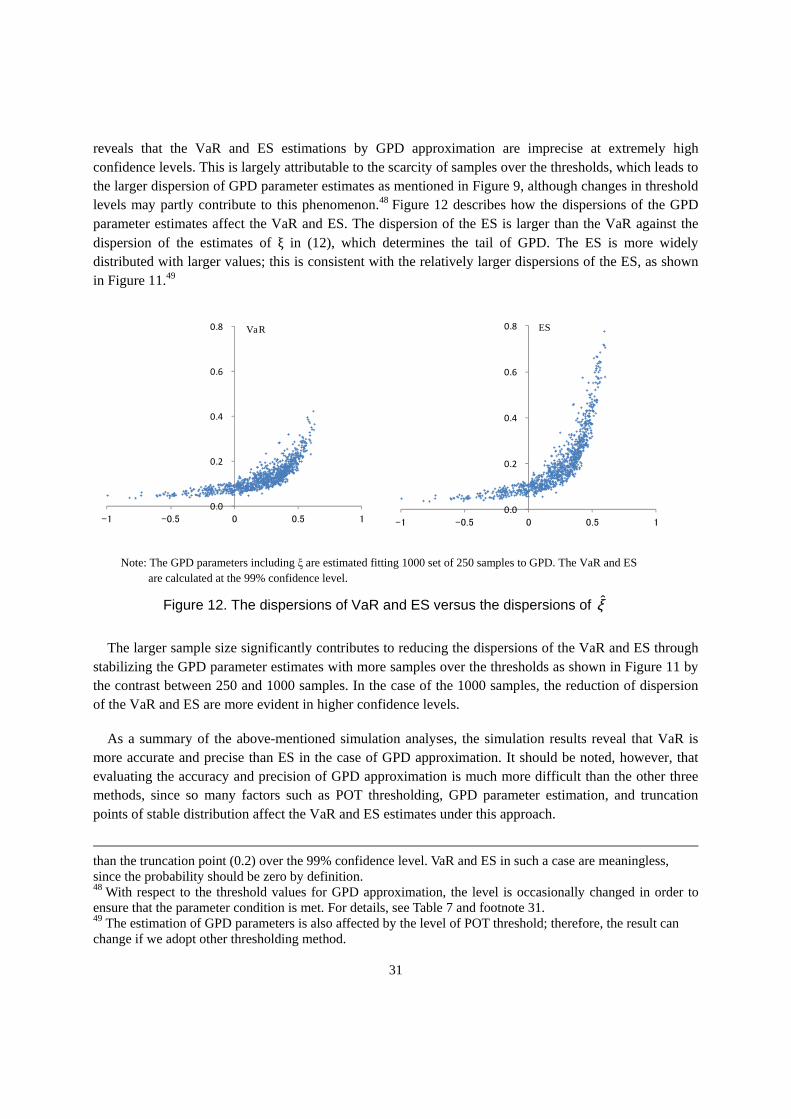
reveals that the VaR and ES estimations by GPD approximation are imprecise at extremely high confidence levels. This is largely attributable to the scarcity of samples over the thresholds, which leads to the larger dispersion of GPD parameter estimates as mentioned in Figure 9, although changes in threshold levels may partly contribute to this phenomenon.48 Figure 12 describes how the dispersions of the GPD parameter estimates affect the VaR and ES. The dispersion of the ES is larger than the VaR against the dispersion of the estimates of ξ in (12), which determines the tail of GPD. The ES is more widely distributed with larger values; this is consistent with the relatively larger dispersions of the ES, as shown in Figure 11.49

Note: The GPD parameters including ξ are estimated fitting 1000 set of 250 samples to GPD. The VaR and ES are calculated at the 99% confidence level.

Figure 12. The dispersions of VaR and ES versus the dispersions of ξ̂

The larger sample size significantly contributes to reducing the dispersions of the VaR and ES through stabilizing the GPD parameter estimates with more samples over the thresholds as shown in Figure 11 by the contrast between 250 and 1000 samples. In the case of the 1000 samples, the reduction of dispersion of the VaR and ES are more evident in higher confidence levels.

As a summary of the above-mentioned simulation analyses, the simulation results reveal that VaR is more accurate and precise than ES in the case of GPD approximation. It should be noted, however, that evaluating the accuracy and precision of GPD approximation is much more difficult than the other three methods, since so many factors such as POT thresholding, GPD parameter estimation, and truncation points of stable distribution affect the VaR and ES estimates under this approach.

than the truncation point (0.2) over the 99% confidence level. VaR and ES in such a case are meaningless, since the probability should be zero by definition. 48 With respect to the threshold values for GPD approximation, the level is occasionally changed in order to ensure that the parameter condition is met. For details, see Table 7 and footnote 31. 49 The estimation of GPD parameters is also affected by the level of POT threshold; therefore, the result can change if we adopt other thresholding method.

ξ ξ 0.0

0.2

0.4

0.6

0.8

-1 -0.5 0 0.5 1

VaR

0.0

0.2

0.4

0.6

0.8

-1 -0.5 0 0.5 1

ES

32

4.1.3 Historical simulation

Figure 13 summarizes the VaR and ES estimation by historical simulation. The average curve of the VaR generally fits well in all sample sizes; however, underestimation was observed for the VaR and ES at higher-than-99% confidence levels, even in the 1000 sample size. As for the bias of the VaR by historical simulation, both under- and overestimation are expected, as mentioned in 3.4.3. The simulation result indicates not the overestimation but the underestimation, which is consistent with the simulation results by Inui (2003) and Ando (2004). This is mainly because our sampling distribution is similar to the ones used in their simulations in terms of fat-tailness. The underestimation is more evident in ES. The average curve of the ES clearly shows underestimation even at lower confidence levels; the underestimation bias increases as confidence level rises. A wider divergence is observed in the 250 sample size compared to the 1000 sample size. This result is also consistent with the simulation analysis by Kim (2010).

We explained earlier that the approximation by historical simulation can be distorted when the sample size is small, as shown in 3.4.3. In the 250 sample size, the VaR and ES at the 99.7% confidence level are equal to those at 99.9%: they do not respond to changes in confidence levels at such an extreme tail as expected. Further, they match the maximum loss due to lower resolution of percentile points. Under such circumstances, increasing the confidence level up to much higher levels like 99.97% is meaningless.

As for the precision of the VaR and ES by historical simulation, as expected, the dispersions of the two risk measures increase as the confidence level rises. The 95% confidence interval as well as the standard deviation is larger at higher confidence levels as in the GPD approximation case. The confidence interval of ES is relatively larger than VaR; this means that ES is less stable compared to VaR. Specifically, the confidence interval of ES is significantly large even at lower confidence levels; for example, under the 98% confidence level in the 250 sample size. Increasing the sample size from 250 to 1000 apparently contributes to improving the precision of VaR and ES with a narrower confidence interval, although the tendency of declining precision, as mentioned above, still exists.

33

Figure 13. VaR and ES by historical simulation

4.1.4 Kernel smoothing

Figure 14 summarizes the VaR and ES estimation by kernel smoothing. The simulation results of kernel smoothing are very similar to those of historical simulation for both VaR and ES; the analysis described in the previous section is essentially valid for kernel smoothing. An important difference that should be mentioned is that VaR and ES at very high confidence levels like 99.7% in the 250 sample size are not equal to the maximum loss (Figure 14, left), unlike under historical simulation. Both of the risk measures increase, albeit marginally, when the confidence level rises to such a high level. This means that VaR and ES respond to changes in confidence levels at the extreme tail due to the kernel smoothing effect.

95 96 97 98 99 100

0.05

0.10

0.15

VaR by historical simulation(mean of 1000 sets, n=250)

MeanStandard deviation95% intervalTruncated stable

95 96 97 98 99 100

0.05

0.10

0.15

VaR by historical simulation(mean of 1000 sets, n=1000)

MeanStandard deviation95% intervalTruncated stable

95 96 97 98 99 100

0.05

0.10

0.15

ES by historical simulation(mean of 1000 sets, n=250)

MeanStandard deviation95% intervalTruncated stable

95 96 97 98 99 100

0.05

0.10

0.15

ES by historical simulation(mean of 1000 sets, n=1000)

MeanStandard deviation95% intervalTruncated stable

34

The smoothing effect of the densities at the tail area by kernel smoothing clearly contributes to avoiding the lower resolution problem observed in historical simulation. The effect is, however, limited in magnitude, since the density estimated by the normal kernel decreases rapidly at the tail area.

The average curve of the VaR generally fits well in both 250 and 1000 sample sizes. The curves are quite similar to the ones by historical simulation except for the difference mentioned above. The average curve of the ES shows underestimation similar to the ES by historical simulation. The bias also increases as confidence level rises. It should be noted, however, that the degree of underestimation is smaller, especially at greater-than-98% confidence levels, than historical simulation in any sample size. The increase in the sample size from 250 to 1000 apparently contributes to reducing the underestimation bias. These findings are consistent with the analyses by Chen and Tang (2005), Chen (2007), and Yu et al. (2010).

As for precision, the 95% confidence interval of kernel smoothing gets narrower for both VaR and ES as the confidence level rises, while the larger sample size clearly contributes to improving the precision of VaR and ES. These findings are also consistent with those of the studies mentioned above.

35

Figure 14. VaR and ES by kernel smoothing

4.2 Relative performance

4.2.1 Normalized (relative) bias

Figure 15 summarizes the normalized biases of VaR and ES estimated by the four methods. The relative measure of bias is defined as the ratio of the estimated VaR or ES to the benchmark VaR or ES. This ratio can be regarded as a distance from the benchmark; therefore, the smaller, the better. As shown in Figure 15, the dotted horizontal line starting from 1.0 on the y-axis is the benchmark line. If the curve of VaR or ES fits this line well, it means that the risk measure is accurately estimated without bias at

95 96 97 98 99 100

0.05

0.10

0.15

0.20

VaR by kernel smoothing(mean of 1000 sets, n=250)

MeanStandard deviation95% intervalTruncated stable

95 96 97 98 99 100

0.05

0.10

0.15

VaR by kernel smoothing(mean of 1000 sets, n=1000)

MeanStandard deviation95% intervalTruncated stable

95 96 97 98 99 100

0.05

0.10

0.15

0.20

ES by kernel smoothing(mean of 1000 sets, n=250)

MeanStandard deviation95% intervalTruncated stable

95 96 97 98 99 100

0.05

0.10

0.15

0.20

ES by kernel smoothing(mean of 1000 sets, n=1000)

MeanStandard deviation95% intervalTruncated stable

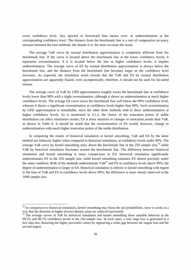
36

every confidence level. Any upward or downward bias means over- or underestimation at the corresponding confidence level. The distance from the benchmark line is a sort of comparative accuracy measure between the four methods: the shorter it is, the more accurate the result.

The average VaR curve by normal distribution approximation is completely different from the benchmark line. If the curve is located above the benchmark line at the lower confidence levels, it represents overestimation; if it is located below the line at higher confidence levels, it implies underestimation. The average curve of ES by normal distribution approximation is always below the benchmark line, and the distance from the benchmark line becomes larger as the confidence level increases. As expected, the simulation result reveals that the VaR and ES by normal distribution approximation are apparently biased, even asymptotically; therefore, it should not be used for fat-tailed returns.

The average curve of VaR by GPD approximation roughly traces the benchmark line at confidence levels lower than 98% with a slight overestimation, although it shows an underestimation at much higher confidence levels. The average ES curve traces the benchmark line well below the 99% confidence level, whereas it shows a significant overestimation at confidence levels higher than 99%. Such overestimation by GPD approximation is remarkable, since the other three methods tend to show underestimation at higher confidence levels. As is mentioned in 4.1.2, the choice of the truncation points of stable distribution can affect simulation results; ES is more sensitive to changes in truncation points than VaR, as shown in Table 8. It should be noted that the overestimation of ES would, however, change to underestimation with much higher truncation points of the stable distribution.

In comparing the results of historical simulation to kernel smoothing, VaR and ES by the latter method are relatively higher when compared to historical simulation, at confidence levels under 99%. The average VaR curve by kernel smoothing stays above the benchmark line in the 250 sample size,50 while VaR by historical simulation fluctuates around the benchmark line. The difference between historical simulation and kernel smoothing is more conspicuous in ES: historical simulation significantly underestimates ES in the 250 sample size, while kernel smoothing estimates ES almost precisely under the same condition. Both of the methods underestimate VaR51 and ES at confidence levels above 99%; the degree of underestimation is larger in ES. Historical simulation is inferior to kernel smoothing with regard to the bias of VaR and ES at confidence levels above 99%; the difference is more clearly observed in the 1000 sample size.

50 In comparison to historical simulation, kernel smoothing may boost the tail probabilities, since it works in a way that the densities in higher (lower) density areas are reduced (increased). 51 The average curves of VaR by historical simulation and kernel smoothing show unstable behavior at the 99.5% and 99.7% confidence levels in the 250 sample size. In such cases, a very large loss is generated in a few data sets, distorting the higher percentile values by registering a wider gap between the largest loss and the second largest.

37

Figure 15. Relative comparison of VaR and ES to the benchmark

As a summary of the earlier analysis, we can conclude that the three methods, namely, historical simulation, GPD approximation, and kernel smoothing show the same level of estimation performance in terms of bias. The normal distribution approximation is far behind those methods as initially expected. More specifically, kernel smoothing might be preferable to the other two methods due to the smaller bias of VaR and ES at higher confidence levels in 1000 samples.

95 96 97 98 99 100

0.6

0.8

1.0

Relative level of VaR(truncated stable=1.0, mean of 1000 sets, n=250)

Normal distributionGPDHistorical simulationKernel smoothing

95 96 97 98 99 100

0.6

0.8

1.0

1.2

Relative level of VaR(truncated stable=1.0, mean of 1000 sets, n=1000)

Normal distributionGPDHistorical simulationKernel smoothing

95 96 97 98 99 100

0.4

0.6

0.8

1.0

1.2

Relative level of ES(truncated stable=1.0, mean of 1000 sets, n=250)

Normal distributionGPDHistorical simulationKernel smoothing

95 96 97 98 99 100

0.4

0.6

0.8

1.0

1.2

Relative level of ES(truncated stable=1.0, mean of 1000 sets, n=1000)

Normal distributionGPDHistorical simulationKernel smoothing

38

4.2.2 Coefficient of variation

Figure 16 summarizes the coefficients of variation (CV) of VaR and ES estimated by the four methods. CV is defined as the ratio of the standard deviation to the mean of VaR or ES over the sample sets, which represents a normalized measure of dispersion of VaR or ES. It shows the extent of variability in relation to the mean of VaR or ES. A smaller CV implies higher precision of the risk measure.

The CVs of VaR and ES by normal distribution approximation are not responsive to the changes in confidence levels, as shown by the horizontal lines in Figure 16. The CV levels of VaR and ES decline when the sample size increases from 250 to 1000, owing to a higher precision of sample variance estimation. Even if the CVs of normal distribution approximation are smaller and stable, irrespective of confidence levels, the VaR and ES are still of little use, since they are biased, even asymptotically as mentioned in 4.1.1.

The CV of VaR by GPD approximation is lower than that of historical simulation and kernel smoothing, respectively at below the 99.9% confidence level, while it reaches the highest level among the four methods at the 99.9% confidence level. GPD approximation seems to be unstable especially at extremely high confidence levels. Such lower precision of GPD approximation is more explicit in the ES calculation (Figure 16, bottom). The CV of ES by GPD approximation records the highest levels at all confidence levels, putting its CV curve above the remaining curves. It gets worse as the confidence level rises. As mentioned earlier, ES by GPD approximation tends to become more unstable than VaR, since ES is far more dependent on the tail probabilities.

Comparing historical simulation with kernel smoothing, the CVs of VaR by kernel smoothing are lower than historical simulation in every sample size, although the difference between the two methods becomes negligible at higher confidence levels. There is no significant difference between historical simulation and kernel smoothing in terms of the CVs of ES. This result is consistent with the analysis by Chen (2007).

39

Figure 16. CVs of VaR and ES

4.3 The ES/VaR ratio

Figure 17 summarizes the ratios of ES to VaR at the same confidence level (ES/VaR) computed by the four methods. The ES/VaR ratio shows the extent to which ES captures tail risk that is not gauged by VaR. This ratio is generally expected to converge to 1 as the confidence level approaches 100%.52 The average curve of the ES/VaR ratio under normal distribution goes down as the confidence level rises, regardless of the sample size. The curve, however, is located far below the benchmark curve at any confidence level, mainly because of underestimation of ES. 52 The convergence level of the ES/VaR ratio of GPD depends on its shape parameter. See footnote 31.

95 96 97 98 99 100

10

15

20

25

30

35

40

45

CV of VaR (mean of 1000 sets, n=250)

Normal diatributionGPDHistorical simulationKernel smoothing

95 96 97 98 99 100

10

15

20

CV of VaR (mean of 1000 sets, n=1000)

Normal diatributionGPDHistorical simulationKernel smoothing

95 96 97 98 99 100

20

30

40

50

60

70

CV of ES (mean of 1000 sets, n=250)

Normal diatributionGPDHistorical simulationKernel smoothing

95 96 97 98 99 100

10

15

20

25

30

35

CV of ES (mean of 1000 sets, n=1000)

Normal diatributionGPDHistorical simulationKernel smoothing

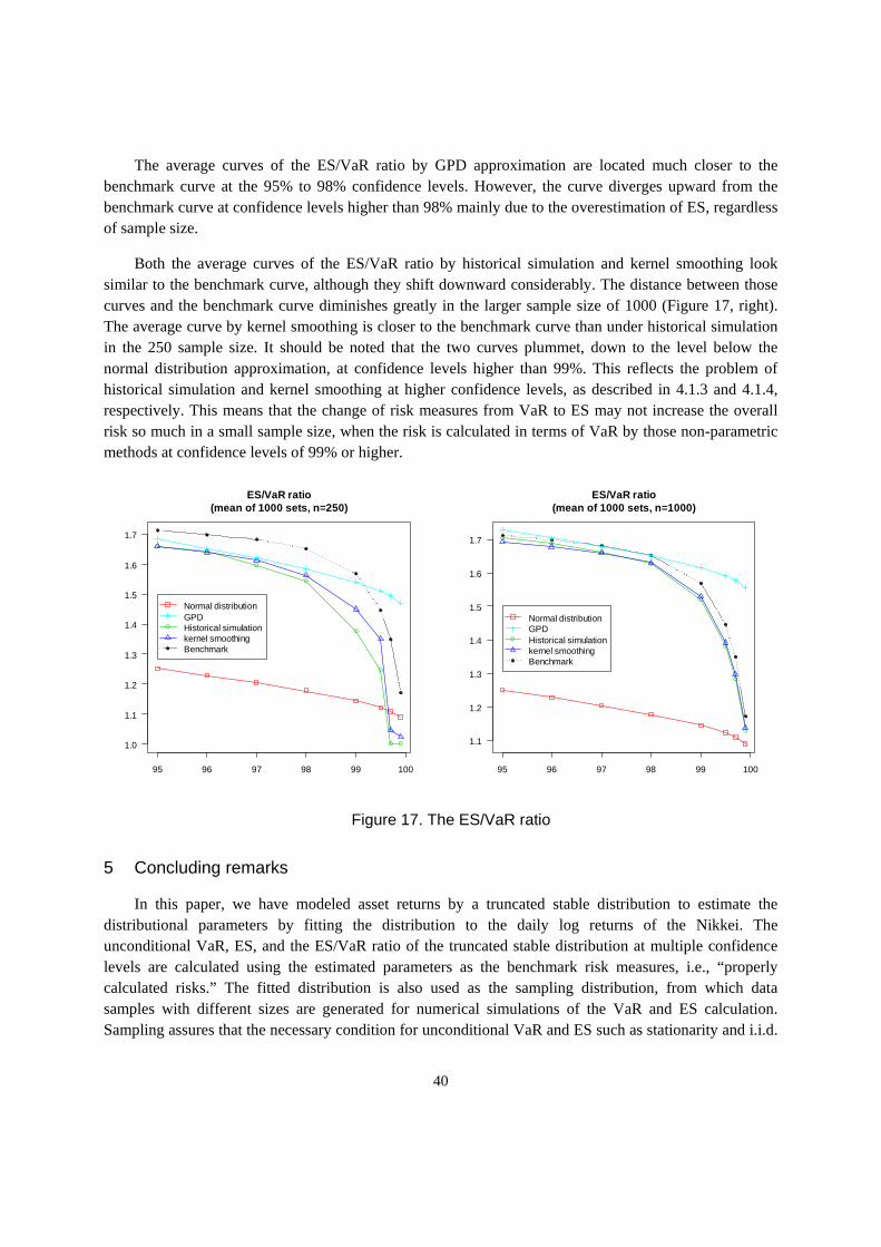
40

The average curves of the ES/VaR ratio by GPD approximation are located much closer to the benchmark curve at the 95% to 98% confidence levels. However, the curve diverges upward from the benchmark curve at confidence levels higher than 98% mainly due to the overestimation of ES, regardless of sample size.

Both the average curves of the ES/VaR ratio by historical simulation and kernel smoothing look similar to the benchmark curve, although they shift downward considerably. The distance between those curves and the benchmark curve diminishes greatly in the larger sample size of 1000 (Figure 17, right). The average curve by kernel smoothing is closer to the benchmark curve than under historical simulation in the 250 sample size. It should be noted that the two curves plummet, down to the level below the normal distribution approximation, at confidence levels higher than 99%. This reflects the problem of historical simulation and kernel smoothing at higher confidence levels, as described in 4.1.3 and 4.1.4, respectively. This means that the change of risk measures from VaR to ES may not increase the overall risk so much in a small sample size, when the risk is calculated in terms of VaR by those non-parametric methods at confidence levels of 99% or higher.

Figure 17. The ES/VaR ratio

5 Concluding remarks

In this paper, we have modeled asset returns by a truncated stable distribution to estimate the distributional parameters by fitting the distribution to the daily log returns of the Nikkei. The unconditional VaR, ES, and the ES/VaR ratio of the truncated stable distribution at multiple confidence levels are calculated using the estimated parameters as the benchmark risk measures, i.e., “properly calculated risks.” The fitted distribution is also used as the sampling distribution, from which data samples with different sizes are generated for numerical simulations of the VaR and ES calculation. Sampling assures that the necessary condition for unconditional VaR and ES such as stationarity and i.i.d.

95 96 97 98 99 100

1.0

1.1

1.2

1.3

1.4

1.5

1.6

1.7

ES/VaR ratio(mean of 1000 sets, n=250)

Normal distributionGPDHistorical simulationkernel smoothingBenchmark

95 96 97 98 99 100

1.1

1.2

1.3

1.4

1.5

1.6

1.7

ES/VaR ratio(mean of 1000 sets, n=1000)

Normal distributionGPDHistorical simulationkernel smoothingBenchmark

41

are all satisfied for the simulation. In the simulation, we compare the four calculation methods: normal distribution approximation, GPD approximation, historical simulation, and kernel smoothing, with regard to bias and precision. It is possible to compare the VaR and ES of the sample data with the benchmark risk measures that are calculated from the sampling distribution. This framework is totally different from back-testing with historical data, in which the true VaR and ES are unknown.

The results of the simulation depict various features of the four methods, underscoring the need for examining whether the selected method is appropriate for the specific fat-tailed return data. The results seem to be convincing, since they also match those of prior studies and theoretical inferences. As for the comparison between the four methods, it is apparent that the VaR and ES by normal distribution approximation are biased, even asymptotically; the ES is far more biased than VaR at any confidence level. The other three methods posted much better performance in terms of bias and precision than normal distribution, although there were some differences among them. It should be noted that they become unstable with smaller sample sizes and/or at higher confidence levels unlike normal distribution approximation. Kernel smoothing is better than the other methods in terms of the smaller biases at higher confidence levels and the improved precision of the ES estimation. GPD approximation is relatively more unstable with larger dispersion, especially in the case of ES.

The key findings of the simulation analysis are summarized below:

i. Bias and precision by sample sizes:

� The biases of VaR and ES by GPD approximation, historical simulation, and kernel smoothing decrease as the sample size increases. The bias of VaR and ES by normal distribution approximation is not responsive to changes in the sample size.

� The increase in the sample size contributes to higher precision for every method.

ii. Bias and precision by confidence levels:

� The dispersion of VaR and ES by normal distribution approximation is not responsive to the changes in confidence levels.

� The dispersion in the other three methods clearly shows an increasing trend as the confidence level rises.

iii. Relative performance of each method against the benchmarks:

� VaR by normal distribution approximation is biased, even asymptotically: it is overestimated at lower confidence levels and underestimated at higher confidence levels. ES is always underestimated: the degree of underestimation is worse at higher confidence levels.

� The relative levels of VaR and ES by the other three methods are almost close to the benchmarks. An underestimation has been detected at confidence levels higher than 99% in those methods except in case of the calculation of ES by GPD approximation. The underestimation is more evident in historical simulation with small-sized samples.

iv. The ES/VaR ratio:

� The ES/VaR ratio at the same confidence level decreases as the confidence level rises in every method.

� The ratio curve of the normal distribution approximation is by far below the benchmark curve.

42

The ratio curve of the other three methods, excluding GPD approximation at higher confidence levels, is close to the benchmark curve; it is much closer in a larger sample size.

� The ratio curve of historical simulation touches upon the bottom line (VaR=ES) at very high confidence levels when the sample size is small (250). This means that the change from VaR to ES has no effect on measured risk.

Calculation of ES is garnering a high level of interest as an alternative risk measure of asset returns versus VaR, as the Basel Committee on Banking Supervision explicitly proposed the use of ES. This paper studies the bias and precision of the VaR and ES calculation methods using numerical simulations.

Through the research result, we have confirmed that each calculation method has distinctive properties, reflecting the type of risk measures, i.e., VaR or ES, as well as the theoretical and methodological backgrounds of the calculation method. Sample data size, confidence level, and computation burden also play key roles in determining the accuracy and precision of a risk measure.

ES is a risk measure that can capture tail risks and are sub-additive unlike VaR; however, it has more problems in terms of bias and precision compared to VaR, especially at higher confidence levels. Increasing the sample size will mitigate this problem considerably. It may not, however, be adequate for unconditional risk modeling to have a very long observation period, since structural changes could be included during the period. Even if ES has merits as mentioned above, stability in calculation is an essential prerequisite for precise risk measurement. VaR seems to be more stable than ES, as revealed by our simulation analysis.

When selecting a risk measure, VaR or ES, all these aspects should be evaluated to determine the most suitable combination of risk measure and calculation method. It should be mentioned that the best choice is rarely available due to tradeoffs between the properties of calculation methods. Thus, it is critically important to determine the rank ordering of the criteria of evaluation, depending on the target asset, in order to make the choice more acceptable.

One of the most difficult elements with regard to the selection of calculation methods of the VaR and ES is how to estimate probability of tail events that have never been observed. The historical simulation method disregards such a possibility, assigning zero probability to any events beyond the maximum loss observed. The normal distribution approximation method assigns a positive but extremely low probability. On the other hand, the GPD distribution method can estimate much higher probability. The selection of the type of distribution depends not only on statistical tests, but also on subjective judgment. This choice significantly affects the level of risk measure; therefore, it should be made after a careful examination of all the factors involved.

We focused on the unconditional model approach in this paper. There is, however, an alternative approach for more responsive risk measurement by the conditional model: it can handle dynamically changing volatilities and the autocorrelation of returns. Under the conditional model framework, back-testing with historical data is frequently used for model validation. Our simulation approach can be implemented in a conditional model framework, although additional modeling and estimation of volatility equation are required. Unlike the back-testing approach that usually focuses on the number of

43

exceedances over a threshold, our approach enables us to analyze precision levels of VaR and ES. Flexible stress scenario setting in simulation is another advantage of our approach, which is not easily available in the case of back-testing with historical data. An examination of this method could form the basis of future research.

44

References

Alexander, C. and Ledermann, D., (2012). “ROM Simulation: Applications to Stress Testing and VaR.” SSRN Electronic Journal.

Alexander, C. and Sheedy, E., (2008). “Developing a stress testing framework based on market risk models.” Journal of Banking & Finance, vol.32(10), pp.2220–2236.

Ando, Y., (2004). “VaR by Historical Simulation: Practical Solutions for Non-Stationarity of Market Returns (in Japanese).” Monetary and Economic Studies, vol.23(2), pp.1–42.

Artzner, P., Delbaen, F., Eber, J.M. and Heath, D., (1999). “Coherent measures of risk.” Mathematical Finance, vol.9(3), pp.203–228.

Balkema, A. and DeHaan, L., (1974). “Residual life time at great age.” The Annals of Probability, vol.2(5), pp.792–804.

Barone-Adesi, G., (2008). “A GARCH option pricing model with filtered historical simulation.” Review of Financial Studies, vol.21(3), pp.1223–1258.

Barone-Adesi, G., Giannopoulos, K. and Vosper, L., (2002). “Backtesting Derivative Portfolios with Filtered Historical Simulation (FHS).” European Financial Management, vol.8(1), pp.31–58.

Basel Committee on Banking Supervision, (2012). “Fundamental review of the trading book - consultative document.”

Borak, S., Misiorek, A. and Weron, R., (2011). “Models for heavy-tailed asset returns.” In P. Cizek, ed. Statistical Tools for Finance and Insurance. Berlin Heidelberg: Springer.

Cai, J., Einmahl, J.H.J., de Haan, L. and Zhou, C., (2012). “Estimation of the Marginal Expected Shortfall: The Mean When a Related Variable is Extreme.” CentER Discussion Paper Series, 2012-080.

Chen, S.X., (2007). “Nonparametric Estimation of Expected Shortfall.” Journal of Financial Econometrics, vol.6(1), pp.87–107.

Chen, S.X. and Tang, C.Y., (2005). “Nonparametric Inference of Value-at-Risk for Dependent Financial Returns.” Journal of Financial Econometrics, vol.3(2), pp.227–255.

Daníelsson, J. and Morimoto, Y., (2000). “Forecasting Extreme Financial Risk: A Critical Analysis of Practical Methods for the Japanese Market.” Monetary and Economic Studies, Institute for Monetary and Economic Studies, Bank of Japan, vol.18(2), pp.25–48.

Dowd, K., (2000). “Assessing VaR Accuracy.” Derivatives Quarterly, vol.6(3), pp.61–63.

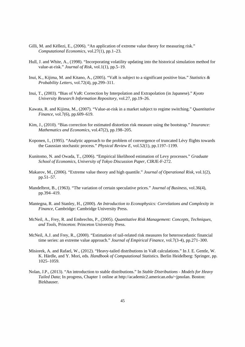
45

Gilli, M. and Këllezi, E., (2006). “An application of extreme value theory for measuring risk.” Computational Economics, vol.27(1), pp.1–23.

Hull, J. and White, A., (1998). “Incorporating volatility updating into the historical simulation method for value-at-risk.” Journal of Risk, vol.1(1), pp.5–19.

Inui, K., Kijima, M. and Kitano, A., (2005). “VaR is subject to a significant positive bias.” Statistics & Probability Letters, vol.72(4), pp.299–311.

Inui, T., (2003). “Bias of VaR: Correction by Interpolation and Extrapolation (in Japanese).” Kyoto University Research Information Repository, vol.27, pp.19–26.

Kawata, R. and Kijima, M., (2007). “Value-at-risk in a market subject to regime switching.” Quantitative Finance, vol.7(6), pp.609–619.

Kim, J., (2010). “Bias correction for estimated distortion risk measure using the bootstrap.” Insurance: Mathematics and Economics, vol.47(2), pp.198–205.

Koponen, I., (1995). “Analytic approach to the problem of convergence of truncated Lévy flights towards the Gaussian stochastic process.” Physical Review E, vol.52(1), pp.1197–1199.

Kunitomo, N. and Owada, T., (2006). “Empirical likelihood estimation of Levy processes.” Graduate School of Economics, University of Tokyo Discussion Paper, CIRJE-F-272.

Makarov, M., (2006). “Extreme value theory and high quantile.” Journal of Operational Risk, vol.1(2), pp.51–57.

Mandelbrot, B., (1963). “The variation of certain speculative prices.” Journal of Business, vol.36(4), pp.394–419.

Mantegna, R. and Stanley, H., (2000). An Introduction to Econophysics: Correlations and Complexity in Finance, Cambridge: Cambridge University Press.

McNeil, A., Frey, R. and Embrechts, P., (2005). Quantitative Risk Management: Concepts, Techniques, and Tools, Princeton: Princeton University Press.

McNeil, A.J. and Frey, R., (2000). “Estimation of tail-related risk measures for heteroscedastic financial time series: an extreme value approach.” Journal of Empirical Finance, vol.7(3-4), pp.271–300.

Misiorek, A. and Rafael, W., (2012). “Heavy-tailed distributions in VaR calculations.” In J. E. Gentle, W. K. Härdle, and Y. Mori, eds. Handbook of Computational Statistics. Berlin Heidelberg: Springer, pp. 1025–1059.

Nolan, J.P., (2013). “An introduction to stable distributions.” In Stable Distributions - Models for Heavy Tailed Data; In progress, Chapter 1 online at http://academic2.american.edu/~jpnolan. Boston: Birkhauser.

46

Pickands, J., (1975). “Statistical inference using extreme order statistics.” Annals of Statistics, vol.3, pp.119–131.

Rachev, S., Kim, Y., Bianchi, M. and Fabozzi, F., (2011). Financial Models with Lévy Processes and Volatility Clustering, New Jersey: Wiley.

Scaillet, O., (2005). “Nonparametric estimation of conditional expected shortfall.” Insurance and Risk Management Journal, vol.74, pp.639–660.

Sheather, S.J. and Marron, J.S., (1990). “Kernel Quantile Estimators.” Journal of the American Statistical Association, vol.85(410), p.410.

Silverman, B.W., (1986). Density Estimation for Statistics and Data Analysis, New York: Chapman & Hall.

Yamai, Y. and Yoshiba, T., (2002). “Comparative Analyses of Expected Shortfall and Value-at-Risk: Their Estimation Error, Decomposition, and Optimization.” Monetary and Economic Studies, vol.20(1), pp.87–122.

Yoshiba, T., (2013). “Risk Aggregation by Copula with Stressed Condition.” Bank of Japan Working Paper, 13-E-12.

Yu, K., Ally, A. and Yang, S., (2010). “Kernel quantile-based estimation of expected shortfall.” Journal of Risk, vol.12(4), pp.15–32.