benchmarking default prediction models: pitfalls - roger m stein

Journal of Risk Model Validation (77–113) Volume 1/Number 1, Spring 2007

Benchmarking default prediction models:pitfalls and remedies in model validation

Roger M. SteinMoody’s Investors Service, 99 Church Street, New York, NY 10007, USA;email: [email protected]

We discuss the components of validating credit default models with a focuson potential challenges to making inferences from validation under real-world conditions. We structure the discussion in terms of: (a) the quantitiesof interest that may be measured (calibration and power) and how they canresult in misleading conclusions if not taken in context; (b) a methodologyfor measuring these quantities that is robust to non-stationarity both interms of historical time periods and in terms of sample firm composition;and (c) techniques that aid in the interpretation of the results of suchtests. The approaches we advocate provide means for controlling for andunderstanding sample selection and variability. These effects can in somecases be severe and we present some empirical examples that highlightinstances where they are and can thus compromise conclusions drawn fromvalidation tests.

1 INTRODUCTION

A model without sufficient validation is only a hypothesis. Without adequateobjective validation criteria and processes, the benefits of implementing and usingquantitative risk models cannot be fully realized. This makes reliable validationtechniques crucial for both commercial and regulatory purposes.

As financial professionals and regulators become more focused on credit riskmeasurement, they have become similarly interested in credit model validationmethodologies. In the case of default models, validation involves examining thegoodness of the model along two broad dimensions: model power and modelcalibration. In practice, measuring these quantities can be challenging.

Power describes how well a model discriminates between defaulting (“Bad”)and non-defaulting (“Good”) firms. For example, if two models produced ratingsof “Good” and “Bad”, the more powerful model would be the one that had ahigher percentage of defaults (and a lower percentage of non-defaults) in its “Bad”

This article was originally released as a working paper (Stein (2002)). The current version hasbeen updated to reflect both comments the author has received since 2002 and new results thathave emerged since the first draft was circulated. I wish to thank Jeff Bohn, Greg Gupton,Ahmet Kocagil, Matt Kurbat, Jody Rasch, Richard Cantor, Chris Mann, Douglas Lucas, NeilReid and Phil Escott for the valuable input I received in writing the first draft. I had very usefulconversations with David Lando, Alan White and Halina Frydman as well. Any errors are, ofcourse, my own.

77

78 R. M. Stein

category and had a higher percentage of non-defaults in its “Good” category. Thistype of analysis can be summarized with contingency tables and power curves.

Calibration describes how well a model’s predicted probabilities agree withactual outcomes. It describes how close the model’s predicted probabilities matchactual default rates. For example, if there were two models A and B that eachpredicted the two rating classes “Good” and “Bad”, and the predicted probabilityof default for A’s “Bad” class were 5% while the predicted probability of defaultfor B’s “Bad” class were 20%, we might examine these probabilities to determinehow well they matched actual default rates. If we looked at the actual default ratesof the portfolios and found that 20% of B’s “Bad” rated loans defaulted while1% of A’s did, B would have the more accurate probabilities since its predicteddefault rate of 20% closely matches the observed default rate of 20%, while A’spredicted default rate of 5% was very different to the observed rate of 1%. (Ofcourse, testing on identical portfolios, were that possible, would be even better.)This type of analysis can be summarized by means of likelihood measures.

The statistical and econometrics literature on model selection and modelvalidation is broad1 and a detailed discussion is beyond the scope of this article.However, measures of “goodness of fit” are in-sample measures and as such, whileuseful during model construction and factor selection, do not provide sufficientinformation about the application of a model to real-world business problems.These more traditional measures are necessary, although not sufficient, for modelsto be useful.

The methodology described here brings together several streams of the valida-tion literature that we have found useful in evaluating quantitative default models.

In this article we discuss various methods for validating default risk modelsduring the development process and discuss cases in which they may break down.We discuss our approach along three lines:

1. what to measure;2. how to measure it; and3. how to interpret the results.

We then make some recommendations about how these factors can be used toinform model selection.

These techniques are most useful in the context of model development whereample data is available. Although they also have implications for the validation ofthird-party models and other internal rating systems by banks and others, in somecases data limitations may make their application difficult in these situations andother approaches may be more suitable. That said, we feel that these techniquesprovide several validation components that represent best practices in modeldevelopment.

The remainder of this article proceeds as follows: Section 2 describes somecommon measures of model performance and discusses their applicability to

1See, for example, Burnham and Anderson (1998) or Greene (2000).

Journal of Risk Model Validation Volume 1/Number 1, Spring 2007

Benchmarking default prediction models: pitfalls and remedies in model validation 79

various aspects of model validation; Section 3 describes the validation approachcalled “walk-forward” testing that controls for model overfitting and permits ananalysis of the robustness of the modeling method through time; in Section 4we discuss some of the practical concerns relating to sample selection and biasthat can arise when testing models on empirical data, we also discuss how thedefinition of validation can be broadened to answer a variety of other questions;and in the concluding section we provide a summary and suggest some generalguidelines for validation work.

2 WHAT TO MEASURE: SOME METRICS OF MODEL PERFORMANCE

This section reviews a variety of measures that assess the goodness of a modelwith respect to its ability to discriminate between defaulting and non-defaultingfirms (its power), as well as the goodness of a model with respect to predicting theactual probabilities of default accurately (its calibration).

We begin by looking at simple tools for examining power. These are useful forproviding an intuitive foundation but tend to be limited in the information theyprovide. We go on to show how these measures can be extended into more generalmeasures of model power.

We next look at tools for comparing the calibration of competing models interms of a model’s ability to accurately predict default rates. This is done bycomparing conditional predictions of default (model predicted probabilities) toactual default outcomes. We begin with a simple example that compares thepredicted average default rates of two models given a test data set, and then extendthis to a more general case of the analysis of individual predicted probabilities,based on firm-specific input data.

We also discuss the potential limitations of power and calibration tests.

2.1 Ranking and power analysis

2.1.1 Contingency tables: simple measures of model powerPerhaps the most basic tool for understanding the performance of a defaultprediction model is the “percentage right”. A more formal way of understandingthis measure is to consider the number of predicted defaults (non-defaults) andcompare this to the actual number of defaults (non-defaults) experienced. Acommon means of representing this is a simple contingency table or confusionmatrix.

Actual Actualdefault non-default

Bad TP FPGood FN TN

In the simplest case, the model produces only two ratings (Bad/Good). Theseare typically shown along the y-axis of the table with the actual outcomes(default/non-default) along the x-axis. The cells in the table indicate the number

Research Papers www.journalofriskmodelvalidation.com

80 R. M. Stein

of true positives (TP), true negatives (TN), false positives (FP) and false negatives(FN), respectively. A TP is a predicted default that actually occurs; a TN is apredicted non-default that actually occurs (the company does not default). ThisFP is a predicted default that does not occur and a FN is a predicted non-defaultwhere the company actually defaults. The errors of the model are FN and FPshown on the off diagonal. FN represents a Type I error and FP represents aType II error. A “perfect” model would have zeros for both the FN and FPcells, and the total number of defaults and non-defaults in the TP and TN cells,respectively, indicating that it perfectly discriminated between the defaulters andnon-defaulters.

There have been a number of proposed metrics for summarizing contingencytables using a single quantity that can be used as indices of model performance.A common metric is to evaluate the true positive rate as a percentage of the TPand FN, TP/(TP + FN), although many others can be used.2 It turns out that inmany cases the entire table can be derived from such statistics through algebraicmanipulation, due to the complimentary nature of the cells.

Note that in the case of default models that produce more than two ratings orthat produce continuous outputs, such as probabilities, a particular contingencytable is only valid for a specific model cutoff point. For example, a bank mighthave a model that produces scores from 1 to 10. The bank might decide that itwill only underwrite loans to firms with model scores better than 5 on the 1 to 10scale. In this case, the TP cell would represent the number of defaulters whoseinternal ratings were worse than 5 and the FP would represent the number of non-defaulters worse than 5. Similarly, the FN would be all defaulters with internalratings better than 5 and the TN would be the non-defaulters better than 5.

It is the case that for many models, different cutoffs will imply different relativeperformances. Cutoff “a” might result in a contingency table that favors model A,while cutoff “b” might favor model B, and so on. Thus, using contingency tables,or indices derived from them, can be challenging due to the relatively arbitrarynature of cutoff definition. This also makes it difficult to assess the relativeperformance of two models when a user is interested not only in strict cutoffs,but in relative ranking, for example when evaluating a portfolio of credits or auniverse of investment opportunities.

2.1.2 CAP plots, ROC curves and power statistics: more generalmeasures of predictive power

ROC (relative or receiver operating characteristic) curves (Green and Swets(1966); Hanley (1989); Pepe (2002); and Swets (1988; 1996)), generalize con-tingency table analysis by providing information on the performance of a modelat any cutoff that might be chosen. They plot the FP rate against the TP rate forall credits in a portfolio.

2For example, Swets (1996) lists 10 of these and provides an analysis of their correspondenceto each other.



ROCs are constructed by scoring all credits and ordering the non-defaultersfrom worst to best on the x-axis and then plotting the percentage of defaultsexcluded at each level on the y-axis. So the y-axis is formed by associatingevery score on the x-axis with the cumulative percentage of defaults with a scoreequal to or worse than that score in the test data. In other words, the y-axis givesthe percentage of defaults excluded as a function of the number of non-defaultsexcluded.

A similar measure, a CAP (Cumulative Accuracy Profile) plot (Sobehart et al2000), is constructed by plotting all of the test data from “worst” to “best” on thex-axis. Thus, a CAP plot provides information on the percentage of defaulters thatare excluded from a sample (TP rate), given that we exclude all credits, Good andBad, below a certain score.

CAP plots and ROC curves convey the same information in slightly differentways. This is because they are geared to answering slightly different questions.

CAP plots answer the question3

“How much of an entire portfolio would a model have to exclude toavoid a specific percentage of defaulters?”

ROC curves use the same information to answer the question

“What percentage of non-defaulters would a model have to excludeto exclude a specific percentage of defaulters?”

The first question tends to be of more interest to business people, while the secondis somewhat more useful for an analysis of error rates.4 In cases where defaultrates are low (ie, 1–2%), the difference can be slight and it can be convenient tofavor one or the other in different contexts. The Type I and Type II error ratesfor the two are related through an identity involving the sample average defaultprobability and sample size (see Appendix A).

Although CAP plots are the representation typically used in practice by financeprofessionals, more has been written on ROC curves, primarily from the statisticsand medical research communities. As a result, for the remainder of this section,we will refer to ROC curves, because they represent the same information as CAPsbut are more consistent with the existing literature.

ROC curves generalize the contingency table representation of model perfor-mance across all possible cutoff points (see Figure 1).

With knowledge of the sample default rate and sample size, the cells of thetable can be filled in directly. If there are ND non-defaulting companies in thedata set and D defaulting companies then the cells are given as follows.5

3In statistical terms, the CAP curve represents the cumulative probability distribution of defaultevents for different percentiles of the risk score scale.4CAP plots can also be more easily used for direct calibration by taking the marginal, ratherthan cumulative, distribution of defaults and adjusting for the true prior probability of default.5Note that D can be trivially calculated as rP, where r is the sample default rate and P is thenumber of observations in the sample. Similarly ND can be calculated as P(1 − r).


82 R. M. Stein

FIGURE 1 Schematic of a ROC showing how all four quantities of a contingencytable can be identified on a ROC curve. Each region of the x- and y-axes have aninterpretation with respect to error and success rates for defaulting (FP and TP)and non-defaulting (FN and TN) firms.

FN%

TP%

FP%

TN%

Non-defaults ordered by model score percentile

Pct

. D

efa

ults

0 20 40 60 80 100

0.0

0.2

0.4

0.6

0.8

1.0

Actual Actualdefault non-default

Bad TP%∗D FP%∗NDGood FN%∗D TN%∗ND

Every cutoff point on the ROC curve gives a measure of Type I and Type IIerror as shown above. In addition, the slope of the ROC curve at each point onthe curve is also a likelihood ratio of the probability of default to non-default fora specific model’s score (Green and Swets (1966)).

Importantly, for validation in cases where the ROC curve of one model isstrictly dominated by the ROC of a second (the second lies above the first at allpoints), the second model will have unambiguously lower error for any cutoff.6

6While often used in practice, cutoff criteria are most appropriate for relatively simpleindependent decisions. The determination of appropriate cutoff points can be based on businessconstraints (eg, there are only enough analysts to follow x% of the total universe), but theseare typically sub-optimal from a profit maximization perspective. A more rigorous criterion canbe derived with knowledge of the prior probabilities and the cost function, defined in terms ofthe costs (and benefits) of FN and FP (and TN and TP). For example, the point at which theline with slope S, defined below, forms a tangent to the ROC for a model, defines the optimal



A convenient measure for summarizing the ROC curve is the area under theROC (A), which is calculated as the integral of the ROC curve: the proportion ofthe area below the ROC relative to the total area of the unit square. A value of 0.5indicates a random model, and a value of 1.0 indicates perfect discrimination. Asimilar measure, the Accuracy Ratio (AR), can also be calculated for CAP plots(Sobehart et al (2000)).7

If the ROC curves for two models cross, neither dominates the other in all cases.In this situation, the ROC curve with the highest value of A may not be preferredfor a specific application defined by a particular cutoff. Two ROC curves may havethe same value of A, but have very different shapes. Depending on the application,even though the area under the curve may be the same for two models, one modelmay be favored over the other.

For example, Figure 2 shows the ROC curves for two models. The ROC curveseach produce the same value for A. However, they have different characteristics.In this example, model users interested in identifying defaults among the worstquality firms (according to the model) might favor model A because it offersbetter discrimination in this region, while those interested in better differentiationamong medium and high-quality firms might choose model B, which has betterdiscrimination among these firms. For some types of applications it may bepossible to use the two models whose ROC curves cross to achieve higher powerthan either might independently (Provost and Fawcett (2001)), although suchapproaches may not be suitable for credit problems.8

The quantity A also has a convenient interpretation. It is equivalent to theprobability that a randomly chosen defaulting loan will be ranked worse thana randomly chosen non-defaulting loan by a specific model (Green and Swets(1966)). This is a useful quantity that is equivalent to a version of the Wilcoxon(Mann–Whitney) statistic (see, for example, Hanley and McNeil, (1982)).

cutoff (Swets (1996)). In this case, S is defined as follows:

S = d ROC(k)

dk= p(ND)

p(D)

[c(FP) + b(TN)][c(FN) + b(TP)]

where b(·) and c(·) are the benefit and cost functions, p(·) is the unconditional probability of anevent, k is the cutoff and D and ND are defined as before. Stein (2005) develops this approachfurther and eliminates the need for a single cutoff by calculating appropriate fees for any loanranked along the ROC curve.7Engelmann et al (2003) also provide an identity relating the area under the curve (A) to theaccuracy ratio (AR): AR = 2(A − 0.5) (see also Appendix A). Alternative versions of accuracyratios have also been developed to tailor the analysis to problem-specific features that sometimesarise in practice (cf Cantor and Mann (2003)).8The approach proposed by Provost and Fawcett (2001) requires one to choose probabilisticallybetween two models for a particular loan application, where the probabilities are proportional tothe location of an optimal cutoff on the tangent to the two ROC curves of the models. Althoughthis strategy can be shown to achieve higher overall power than either model would on itsown, the choosing process may be inappropriate for credit because the same loan could getdifferent scores if run through the process twice. For applications involving direct marketing,fraud detection, etc, this is not generally an issue; however, in credit-related applications thedrawbacks of this non-determinism may be sufficient to outweigh the benefits of added power.


84 R. M. Stein

FIGURE 2 Two ROCs with the same area but different shapes. The area underthe ROC (A) for each is the same, but the shapes of the ROCs are different. Usersinterested in identifying defaults among the worst firms might favor model A,while those interested in better differentiation among medium and high-qualityfirms might choose model B.

0.0 0.2 0.4 0.6 0.8 1.0

Percentage of non-defaults

0.0

0.2

0.4

0.6

0.8

1.0

Model.A

Model.B

ROC curves provide a good deal of information regarding the ability of a creditmodel to distinguish between defaulting and non-defaulting firms. The meaning ofan ROC curve (or a CAP plot) is intuitive and the associated statistic A (or AR) hasa direct interpretation with respect to a model’s discriminatory power. For creditmodel evaluation, where we are typically most concerned with a model’s abilityto rank firms correctly, an ROC curve or CAP plot is more useful than simplecontingency tables because the graphical measures avoid the need to define strictcutoffs and provide more specific information about the regions in which modelpower is highest. As such, they provide much more general measures of modelpower.

It is helpful to think not only in statistical terms, but also in economic terms.Stein (2005) demonstrated that the same machinery to that used to determineoptimal cutoffs in ROC analysis (see footnote 6) can also be used to determinethe fees that should be charged for risky loans at any point on the ROC curve,implying that no loans need be refused. In this way, the ROC directly relatesto loan pricing. Furthermore, this relationship naturally provides a mechanismto determine the economic value of a more powerful model. Stein and Jordão(2003) provided a methodology for evaluating this through data-based simulation



and showed that for a typical bank the value of even a somewhat more powerfulmodel can be millions of dollars. Blöchlinger and Leippold (2006) provided analternative approach that does not require data (given a number of simplifyingassumptions).

ROC curves and CAP plots and their related diagnostics are power statisticsand, as such, do not provide information on the appropriateness of the levels ofpredicted probabilities. For example, using ROC analysis, model scores do notneed to be stated as probabilities of default, but could be letter grades, points ona scale of 1–25, and so on. Scores from 1 to 7 or 10 are common in internal bankrating systems. Models that produce good rankings ordinarily will be selected bypower tests over those that have poorer power even though the meaning of, say, a“6” may not be well defined in terms of probabilities.

Powerful models, without probabilistic interpretations, however, cannot beused in certain risk management applications such as CVAR and capital allocationbecause these applications require probabilities of default. Fortunately, it isusually possible to calibrate a model to historical default probabilities. In the nextsection we examine measures of the accuracy of such calibration.

2.2 Likelihood-based measures of calibration

As used here, likelihood measures9 provide evidence of the plausibility of aparticular model’s probability estimates given a set of empirical data. A likelihoodestimate can be calculated for each model in a set of candidate models and willbe highest for the model in which the predicted probabilities match most closelywith the actual observed data.

The likelihood paradigm can be used to evaluate which hypothesis (or model)among several has the highest support from the data. The agreement of predictedprobabilities with subsequent credit events is important for risk management,pricing and other financial applications, and as a result, modelers often spend afair amount of time calibrating models to true probabilities.

Calibration typically involves two steps. The first requires mapping a modelscore to an empirical probability of default using historical data. For example,the model outputs might be bucketed by score and the default rates for eachscore calculated using an historical database. The second step entails adjustingfor the difference between the default rate in the historical database and the actualdefault rate.10 For example, if the default rate in the database were 2%, but the

9A detailed discussion of likelihood approaches is beyond the scope of this paper. For anintroduction, see Reid (2002), which provides a brief discussion, Edwards (1992), whichprovides more insight and some historical background, or (Royall (1997)), which providesa more technical introduction along with examples and a discussion of numerical issues.Friedman and Cangemi (2001) discuss these measures in the context of credit model validation.10It is not uncommon for these rates to be different due to data gathering and data processingconstraints, particularly when dealing with middle market data from banks data in whichfinancial statements and loan performance data are stored in different systems. In technicalterms, it is necessary to adjust the model prediction for the true prior probability.


86 R. M. Stein

actual default rate were known (through some external source) to be 4%, it wouldbe necessary to adjust the predicted default rates to reflect the true default rate.11

Note that tests of calibration are tests of levels rather than tests of power andas such can be affected if the data used contains highly correlated default eventsor if the data represent only a portion of an economic cycle. This issue can arisein other contexts as well. Although we do not discuss it in detail in this article, itis important to consider the degree to which these may have impact on results (cf,Stein (2006)).

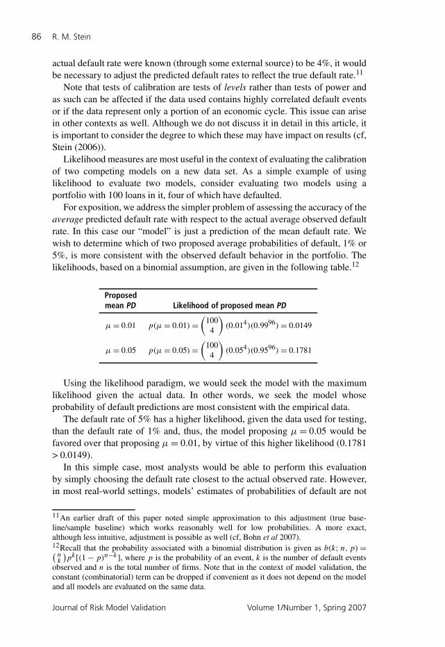
Likelihood measures are most useful in the context of evaluating the calibrationof two competing models on a new data set. As a simple example of usinglikelihood to evaluate two models, consider evaluating two models using aportfolio with 100 loans in it, four of which have defaulted.

For exposition, we address the simpler problem of assessing the accuracy of theaverage predicted default rate with respect to the actual average observed defaultrate. In this case our “model” is just a prediction of the mean default rate. Wewish to determine which of two proposed average probabilities of default, 1% or5%, is more consistent with the observed default behavior in the portfolio. Thelikelihoods, based on a binomial assumption, are given in the following table.12

Proposedmean PD Likelihood of proposed mean PD

µ = 0.01 p(µ = 0.01) =(

1004

)(0.014)(0.9996) = 0.0149

µ = 0.05 p(µ = 0.05) =(

1004

)(0.054)(0.9596) = 0.1781

Using the likelihood paradigm, we would seek the model with the maximumlikelihood given the actual data. In other words, we seek the model whoseprobability of default predictions are most consistent with the empirical data.

The default rate of 5% has a higher likelihood, given the data used for testing,than the default rate of 1% and, thus, the model proposing µ = 0.05 would befavored over that proposing µ = 0.01, by virtue of this higher likelihood (0.1781> 0.0149).

In this simple case, most analysts would be able to perform this evaluationby simply choosing the default rate closest to the actual observed rate. However,in most real-world settings, models’ estimates of probabilities of default are not

11An earlier draft of this paper noted simple approximation to this adjustment (true base-line/sample baseline) which works reasonably well for low probabilities. A more exact,although less intuitive, adjustment is possible as well (cf, Bohn et al 2007).12Recall that the probability associated with a binomial distribution is given as b(k; n, p) =( n

k

)pk[(1 − p)n−k ], where p is the probability of an event, k is the number of default events

observed and n is the total number of firms. Note that in the context of model validation, theconstant (combinatorial) term can be dropped if convenient as it does not depend on the modeland all models are evaluated on the same data.



constant as in the example above, but are conditional on a vector of input variables,x, that describes the company. Appendix B provides a review of the mathematicsthat extend the simple case to the more general case.

For technical reasons, it is convenient to work with the log of the likelihood,�(·), which is a monotonic transformation of the likelihood and thus the largestvalue of the likelihood will be associated with the model that produces the largestvalue for � (model). (Note that this amounts to the value with the least negativenumber.) The model with the highest log likelihood would be the best calibrated.Importantly, note that in this context, the likelihood measure is calculated givenonly a vector of model outputs and a vector of default outcomes. It is not thelikelihood that may have been calculated during the model estimation processand it does not admit information outside of the model predictions and actualoutcomes. This formulation allows it to accommodate out-of-sample testing.

While calibration can be challenging, it is generally far easier to calibrate apowerful model to true default rates than it is to make a weak but well calibratedmodel more powerful.

This fact highlights a drawback of using likelihood measures alone for val-idation. The focus on calibration exclusively can lead likelihood methods toincorrectly reject powerful, but imperfectly calibrated models in favor of weakerbut better calibrated models. This is true even when the poorly calibrated modelcan be “fixed” with a simple adjustment.

To see this, consider an example of two models W and P that are being appliedto an identical portfolio of 11,000 loans with a true default rate of 5%. Assume thatneither model was developed using the test set, so the test is an “out-of-sample”test, such as might be performed by a bank evaluating two credit models on itsown portfolio. The models themselves are very simple, with only two ratings:Good and Bad. The models have been calibrated so each rating has an associatedprobability of default.

The following table gives the log likelihoods for these two example modelsunder this data set. Using the likelihood criterion, we would choose model Wover model P because a difference of 132 in log likelihood is large.13

Model Log likelihood

W −2,184P −2,316

(W) − (P) 132

Now consider how the models that produced these likelihoods performed.The following tables show the number of defaults predicted by each model andthe predicted probabilities under each model for each class, based on the statedcalibration of the two models.

13See Appendix B for details.


88 R. M. Stein

Actual outcome

Model Model PD prediction Default Non-default

W 5.10% Bad 50 9504.90% Good 500 9,500

P 1.50% Bad 549 10.01% Good 1 10,449

Recall that the likelihood approach in this context is being used to determinethe effectiveness of model calibration. Now note that the preferred (under thelikelihood selection paradigm) model W (the weaker model) does a far worsejob separating defaulting firms from healthy ones. It turns out that model W’sactual performance is no different than a random model in that both Good andBad ratings have a 5% probability of default on the test set, and this is the same asthe actual central tendency of the test set. Thus, it does not matter which rating themodel gives, the actual default rate will be the same: the mean for the population(50/1,000 = 500/10,000 = 5%).

In contrast, model P (the more powerful model) demonstrates very goodpower, discriminating almost perfectly between defaulters and non-defaulters.Most lenders, if asked to choose, would select model P because, using this out-of-sample test data set, model P gives high confidence that the bank will identifyfuture defaulters.

Why is model W selected over model P under the likelihood paradigm? It isbecause its probabilities more closely match the observed probabilities of thedata set. Thus, even though it is a random model that results in the same realizedprobability for both Good and Bad classes, this probability is very close to whatis actually observed on average, and thus the model probabilities are more likely,given the data, than those of model P.

On the other hand, model P was miscalibrated and therefore its very powerfulpredictions do not yield the number of defaulters in each class that would beexpected by its predicted probabilities of 1.5% and 0.01%. It is not as wellcalibrated to its actual performance.

Now suppose that the modeler learns that the true prior probabilities of thesample were different than the probabilities in the real population and adjusts themodel output by a (naive) constant factor of two. In this case, the log likelihoodof model P would change to −1,936 and, after this adjustment, model P wouldbe preferred. Note that the model is still badly miscalibrated, but even so, underthe likelihood paradigm, it would now be preferred over model W. Thus, a simple(constant) adjustment to the prior probability results in the more powerful modelbeing better calibrated than model W.

It is reasonable to ask whether there is a similar simple adjustment we canmake to model W to make it more powerful. Unfortunately, there is generally nostraightforward way to do this without introducing new or different variables intothe model or changing the model structure in some other way.

Interestingly, if an analyst was evaluating models using tests of model powerrather than calibration, almost any model would have been chosen over model W.



To see this, consider that model W makes the same prediction for every credit andthus provides no ranking beyond a random one. Thus, model W would be identicalto the random model in a power test. Even a very weak model that still providedslight discrimination would be chosen over model W if the criterion were power.

Note that likelihood measures are designed for making relative comparisonsbetween competing models, not for evaluating whether a specific model is “close”to being correctly calibrated or not. So the best model of a series of candidatemodels might still be poorly calibrated (just less so than the other models). Owingto this, many analysts find it useful to perform other types of tests of calibration aswell. For example, it is often useful to bin a test data set by predicted probabilitiesof default and to then calculate the average probability of default for each bin todetermine whether the predicted default rate is reasonably close to the observeddefault rate. In this case, the analyst can get more direct intuition about theagreement and direction of default probabilities than might be available from thelikelihood paradigm, but may have a less precise quantitative interpretation ofthese results. Both analyses can be useful.

As a whole, the likelihood measures we have discussed here focus on theagreement of predicted probabilities with actual observed probabilities, not on amodel’s ability to discriminate between Goods and Bads. In contrast, a CAP plotor an ROC curve measures the ability of a model to discriminate between Goodsand Bads, but not to accurately produce probabilities of default.

If the goal is to have the most accurate probability estimate, irrespective of theability to discriminate between Good and Bad credits, the maximum likelihoodparadigm will always provide an optimal model selection criterion. However,there is no guarantee that the model selected by the likelihood approach will bethe most powerful or, as the example shows, even moderately powerful.

In contrast, if the goal is to determine which model discriminates best betweendefaulting and non-defaulting firms, tools such as ROC curves CAP plots providea well-established means for doing so. In this case, there are no guarantees on theappropriateness of the probability estimates produced by the model, but we do getan unambiguous measure of the model’s power.14

2.3 The relationship between power and calibration

Importantly, although they measure different things, power and calibration arerelated: the power of a model is a limiting factor on how high a resolution may beachieved through calibration, even when the calibration is done appropriately. Tosee this, consider the following example of four models each with different power:a perfect default predictor, a random default predictor, a powerful, but not perfect

14Both calibration and power analysis can be extended to more involved contexts. For example,likelihood measures can be used to evaluate long run profitability using the Kelly criteria (Kelly(1956)). While exceptions do exist (eg, Bell and Cover (1980)), in general, these criteria arebased on atypical assumptions of a series of sequential single-period decisions rather than theexistence of a portfolio. It is more common for an investor to own a portfolio of assets (eg,loans) and ask whether adding another is desirable.


90 R. M. Stein

FIGURE 3 Calibration curves for four hypothetical models with different power.The more powerful a model is, the better the resolution it can achieve inprobability estimation. Each of these models is perfectly calibrated, given thedata, but they are able to achieve very different levels because of their differingpower. The random model can never generate very high or very low probabilitieswhile the perfect model can generate probabilities that range from zero to one(although none in between). The more powerful model can give broad ranges,while the weaker model can only give narrower ranges.

Perfect Model

Model score

Calib

rate

d P

D

0 20 40 60 80 100

0.0

0.2

0.4

0.6

0.8

1.0

Powerful Model

Model score

Calib

rate

d P

D

0 20 40 60 80 100

0.0

0.2

0.4

0.6

0.8

1.0

Weak Model

Model score

Calib

rate

d P

D

0 20 40 60 80 100

0.0

0.2

0.4

0.6

0.8

1.0

Random Model

Model score

Calib

rate

d P

D

0 20 40 60 80 100

0.0

0.2

0.4

0.6

0.8

1.0

model and a weak, but not random one. Assume that the data used for calibrationis a representative sample of the true population.

Figure 3 shows the calibration curve for these four hypothetical models. In thisexample, we discuss only on the calibration of the very worst score (far left valuesin each graph) that the model produces because the other scores follow the samepattern.

How does the calibration look for the perfect model? In the case of the perfectmodel, the default probability for the worst score will be 1.00 since the modelsegregates perfectly the defaulting and non-defaulting firms, assigning bad scoresto the defaulters. On the other hand, how does this calibration look for the randommodel? In this case, calibrated default probability is equal to the mean default ratefor the population because each score will contain a random sample of defaultsand non-defaults. The other two models lie somewhere between these extremes.



For the powerful model, the calibration can reach levels close to the perfectmodel, but because it does not perfectly segregate all of the defaults in the lowestscore, there are also some non-defaulters assigned the worst score. As a result,even if the model is perfectly calibrated to the data (ie, the calibrated probabilitiesfor each bucket exactly match those in the data set), it cannot achieve probabilitiesof 1.00. Similarly, the weak model performs better than the random model, butbecause it is not very powerful, it gives a relatively flat curve that has a muchsmaller range of values than the powerful model.

This implies that a more powerful model will be able to generate probabilitiesthat are more accurate than a weaker model, even if the two are calibrated perfectlyon the same data set. This is because the more powerful model will generate higherprobabilities for the defaulting firms and lower probabilities for non-defaultingfirms due to its ability to discriminate better between the two groups and thusconcentrate more of the defaulters (non-defaulters) in the Bad (Good) scores.

There is no simple adjustment to the calibration of these models to improvethe accuracy of the probability estimates because they are calibrated as well aspossible, given their power. This does not mean that the probabilities of the weakerand more powerful model are equally accurate, only that they cannot be improvedbeyond their accuracy level through simple calibration unless the power is alsoimproved.15

3 HOW TO MEASURE: A WALK-FORWARD APPROACH TO MODELTESTING

Performance statistics for credit risk models are typically very sensitive to thedata sample used for validation. We have found that tests are most reliable whenmodels are developed and validated using some type of out-of-sample and out-of-time testing.16

Indeed, many models are developed and tested using some form of “hold-outtesting” which can range from simple approaches such as saving some fractionof the data (a “hold-out sample”) for testing after the model is fit, to moresophisticated cross-validation approaches. However, with time varying processessuch as credit,17 hold out testing can miss important model weaknesses notobvious when fitting the model across time because simple hold-out tests do notprovide information on performance through time.

In the following section, we describe a validation framework that accountsfor variations across time and across the population of obligors. It can provide

15Note that the relationship between power and calibration is direct provided that the calibrationmethod involves monotonic transformations of the model output. However, calibration tech-niques that change the ordering of observations (cf, Dwyer and Stein (2005)) do not maintainthe power–calibration relationship described above and can also improve model power.16Out-of-sample refers to observations for firms that are not included in the sample used to buildthe model. Out-of-time refers to observations that are not contemporanious with the trainingsample.17See, for example, Mensah (1984) or Gupton and Stein (2002).


92 R. M. Stein

FIGURE 4 Schematic of out-of-sample validation techniques. Testing strategiesare split based on whether they account for variances across time (horizontalaxis) and across the data universe (vertical axis). Dark circles represent trainingdata and white circles represent testing data. Gray circles represent data thatmay or may not be used for testing. (Adapted from Dhar and Stein (1998).)

Out of sample

Out of time

Out of universe

A

A

A

A

B B

Out of sample Out of sample

Out of time

Out of sample

Out of universe

Acro

ss

un

ive

rs

e

Across time

NO YES

NO

YES

important information about the performance of a model across a range ofeconomic environments.18

This approach is most useful in validating models during development and lesseasily applied where a third-party model is being evaluated or when data is morelimited. That said, the technique is extremely useful for ensuring that a model hasnot been overfit.

3.1 Forms of out-of-sample testing

A schematic of the various forms of out-of-sample testing is shown in Figure 4.The figure splits the model testing procedure along two dimensions: (a) time(along the horizontal axis) and (b) the population of obligors (along the verticalaxis). The least restrictive out-of-sample validation procedure is represented bythe upper-left quadrant and the most stringent by the lower-right quadrant. Theother two quadrants represent procedures that are more stringent with respect toone dimension than the other.

The upper-left quadrant describes the approach in which the testing data formodel validation is chosen completely at random from the full model fitting dataset. This approach to model validation assumes that the properties of the dataremain stable over time (stationary process). As the data is drawn at random, this

18The presentation in this section follows closely that of Dhar and Stein (1998), Stein (1999)and Sobehart et al (2000).



approach validates the model across the population of obligors but does not testfor variability across time.

The upper-right quadrant describes one of the most common testing proce-dures. In this case, data for model fitting is chosen from any time period prior to acertain date and testing data is selected from time periods only after that date. Asmodel validation is performed with out-of-time samples, the testing assumptionsare less restrictive than in the previous case and time dependence can be detectedusing different validation sub-samples. Here it is assumed that the characteristicsof firms do not vary across the population.

The lower-left quadrant represents the case in which the data is segmented intotwo sets containing no firms in common, one set for building the model and theother for validation. In this general situation the testing set is out-of-sample. Theassumption of this procedure is that the relevant characteristics of the populationdo not vary with time but that they may vary across the companies in the portfolio.

Finally, the most robust procedure is shown in the lower-right quadrant andshould be the preferred sampling method for credit risk models. In addition tobeing segmented in time, the data is also segmented across the population ofobligors. Non-overlapping sets can be selected according to the peculiarities ofthe population of obligors and their importance (out-of-sample and out-of-timesampling).

Out-of-sample out-of-time testing is beneficial because it prevents overfittingof the development data set, but also prevents information about future states ofthe world that would not have been available when developing the model frombeing included. For example, default models built before a market crisis may ormay not have predicted default well during and after the crisis, but this cannot betested if the data used to build the model was drawn from periods before and afterthe crisis. Rather, such testing can only be done if the model was developed usingdata prior to the crisis and tested on data from subsequent periods.

As default events are rare, it is often impractical to create a model usingone data set and then test it on a separate “hold-out” data set composed ofcompletely independent data. While such out-of-sample and out-of-time testswould unquestionably be the best way to compare models’ performance if defaultdata was widely available, it is rarely possible in practice. As a result, mostinstitutions face the following dilemma:

• If too many defaulters are left out of the in-sample data set, estimation of themodel parameters will be seriously impaired and overfitting becomes likely.

• If too many defaulters are left out of the hold-out sample, it becomesexceedingly difficult to evaluate the true model performance due to severereductions in statistical power.

3.2 The walk-forward approachIn light of these problems, an effective approach is to “rationalize” the defaultexperience of the sample at hand by combining out-of-time and out-of-sampletests. A testing approach that focuses on this last quadrant and is designed to test


94 R. M. Stein

models in a realistic setting, emulating closely the manner in which the modelsare used in practice, is often referred to in the trading model literature as “walk-forward” testing.

It is important to make clear that there is a difference between walk-forwardtesting and other more common econometric tests of stationary or goodness offit. For example, when testing for goodness of fit of a linear model in economics,it is common to look at an R2 statistic. For more general models, a likelihoodrelated (eg, Akaike’s information criterion (AIC), etc) measure might be used.When testing for the stationarity of an economic process, researchers will oftenuse a Chow test.

The key difference between these statistics and tests and statistics derived fromwalk-forward tests is that statistics such as R2 and AIC and tests such as Chowtests are all in-sample measures. They are designed to test the agreement of theparameters of the model or the errors of the model with the data used to fit themodel during some time period(s). In contrast, walk-forward testing provides aframework for generating statistics that allow researchers to test the predictivepower of a model on data not used to fit it.

The walk-forward procedure works as follows:

(1) Select a year, for example 1997.(2) Fit the model using all the data available on or before the selected year.(3) Once the model’s form and parameters are established for the selected time

period, generate the model outputs for all of the firms available during thefollowing year (in this example, 1998).

(4) Save the prediction as part of a result set.(5) Now move the window up (eg, to 1998) so that all of the data through that

year can be used for fitting and the data for the next year can be used fortesting.

(6) Repeat steps (2) to (5) adding the new predictions to the result set for everyyear.

Collecting all of the out-of-sample and out-of-time model predictions producesa set of model performances. This result set can then be used to analyze theperformance of the model in more detail. Note that this approach simulates, asclosely as possible given the limitations of the data, the process by which themodel will actually be used. Each year, the model is refit and used to predict thecredit quality of firms one year hence. The process is outlined in the lower left ofFigure 5.

In the example below, we used a one-year window. In practice the windowlength is often longer and may be determined by a number of factors includingdata density and the likely update frequency of the model itself, once it is online.

The walk-forward approach has two significant benefits. First, it gives arealistic view of how a particular model would perform over time. Second,it gives analysts the ability to leverage to a higher degree the availability ofdata for validating models. In fact, the validation methodology not only tests a



FIGURE 5 Schematic of the walk-forward testing approach. In walk-forwardtesting, a model is fit using a sample of historical data on firms and tested usingboth data on those firms one year later and data on new firms one year later(upper portion of exhibit). Dark circles represent in-sample data and white circlesrepresent testing data. This approach results in “walk-forward testing” (bottomleft) when it is repeated in each year of the data by fitting the parameters ofa model using data through a particular year, and testing on data from thefollowing year, and then moving the process forward one year. The results ofthe testing for each validation year are aggregated and then may be resampled(lower left) to calculate particular statistics of interest.

1997 1998 1999 2000 . . . . 2005

A

B

A

B

A

B

A

B

A

B

Training set of firms taken at t0

Validation set of original firms in training sample but taken at t

1

Validation set of new firms not in training sample and taken at t

1

}

Resu

lt Set

Prepayment Model

0%

10%

20%

30%

40%

50%

60%

70%

80%

90%

100%

0% 10% 20% 30% 40% 50% 60% 70% 80% 90% 100%

Percent of Portfolio

Pre

pay

men

ts

Model Subpr ime Literature 2 Simple

Accuracy Rat io - Severi ty

0

0.1

0.2

0.3

0.4

0.5

0.6

0.7

Simple Literature Model Subprime

Mean

Sq

uare

d E

rro

r

Performance

Statistics

1997 1998 1999 2000 . . . . 2005

A

B

A

B

A

B

A

B

A

B

A

B

A

B

A

B

A

B



1


1

A

B

A

B

A

B



1


1

}

Resu

lt Set

Prepayment Model

0%

10%

20%

30%

40%

50%

60%

70%

80%

90%

100%

0% 10% 20% 30% 40% 50% 60% 70% 80% 90% 100%


Pre

pay

men

ts


Prepayment Model

0%

10%

20%

30%

40%

50%

60%

70%

80%

90%

100%

0% 10% 20% 30% 40% 50% 60% 70% 80% 90% 100%


Pre

pay

men

ts



0

0.1

0.2

0.3

0.4

0.5

0.6

0.7


Mean

Sq

uare

d E

rro

r


0

0.1

0.2

0.3

0.4

0.5

0.6

0.7


Mean

Sq

uare

d E

rro

r

Performance

Statistics

particular model, but it tests the entire modeling approach. As models are typicallyreparameterized periodically as new data come in and as the economy changes, itis important to understand how the approach of fitting a model, say once a year,and using it in real-time for the subsequent year, will perform. By employingwalk-forward testing, analysts can get a clearer picture of how the entire modelingapproach will hold up through various economic cycles.

Two issues can complicate the application of the walk-forward approach. Thefirst is the misapplication of the technique through the repeated use of the walk-forward approach while developing the model (as opposed to testing a single finalmodel). In the case where the same “out-of-sample” data is used repeatedly togarner feedback on the form of a candidate model as it is being developed, theprinciple of “out-of-time” is being violated.


96 R. M. Stein

The second complication can arise when testing models that have continuouslyevolved over the test period. For example, banks often adjust internal ratingmodels to improve them continuously as they use them. As a result it is oftenimpossible to recreate the model, as it would have existed at various points in thehistorical test period, so it can be difficult to compare the model with others on thesame test data set. In such situations, it is sometimes feasible to test the model onlyin a period of time after the last change was made. Such situations are reflected inthe upper-right quadrant of Figure 4. This approach tends to limit the number ofdefaults available and as a result it can be difficult to draw strong conclusions (seeSection 4).

In light of the complications that can result in limitations on test samples, it isof interest to develop techniques for interpreting the results of validation exercises.In the next section we discuss some of these.

4 HOW TO INTERPRET PERFORMANCE: SAMPLE SIZE, SAMPLESELECTION AND MODEL RISK

Once a result set of the type discussed in Section 3 is produced and performancemeasures as described in Section 2 are calculated, the question remains of howto interpret these performance measures. Performance measures are sensitive tothe data set used to test a model, and it is important to consider how they areinfluenced by the characteristics of the particular data set used to evaluate themodel.

For problems involving “rare” events (such as credit default), it is the number ofoccurrences of the rare event more than the total number of observations that tendsto drive the stability of performance measures. For example, if the probability ofdefault in a population is of the order of 2% and we test a model using a sampleof 1,000 firms, only about 20 defaults will be in the data set. In general, had themodel been tested using a different sample that included a different 20 defaults,or had the model used only 15 of the 20 defaults, we could often observe quitedifferent results.

In addition to the general variability in a particular data set, a sample drawnfrom one universe (eg, public companies) may give quite different results thanwould have been observed on a sample drawn from a different universe (eg, privatecompanies). Recall again the discussion of Figure 4.

In most cases, it is impossible to know how a model will perform on a differentsample than the one at hand (if another sample were available, that sample wouldbe used as data for testing as well). The best an analyst can do is size the magnitudeof the variability that arises due to sampling effects.

We next focus on two types of uncertainty that can arise in tests using empiricaldata.

• There is a natural variability in any sample chosen from the universe ofdefaulting and non-defaulting firms. Depending on the number of defaultingand non-defaulting firms, this variability can be relatively small or quitelarge. Understanding this variability is essential to determining whether



differences in the performance of two models are spurious or significant.One approach to sizing this variability is through the use of resamplingtechniques, which are discussed, along with examples, in Section 4.1. Asexpected, the smaller the number of defaults, the higher the variability.

• There can be an artificial variability that is created when samples are drawnfrom different populations or universes, as in the case when a model is testedon a sample drawn from a population that is different than the populationthat the model will be applied to. For example, a bank may wish to evaluatea private firm default model but only have access to default data for publiccompanies. In this case, analysts will have less certainty and it will beharder to size the variably of testing results. We briefly discuss this typeof variability in Section 4.2 where we try to give some indication for thedifferences in model performance when samples are drawn from differentpopulations. We provide an example of the performance of the same modelon samples drawn from different populations.

It is often the case that competing models must be evaluated using only thedata that an institution has on hand and this data may be limited. This limitationcan make it difficult to differentiate between good and mediocre models. Thechallenge faced by many institutions is to understand these limitations and to usethis understanding to design tests that lead to informed decisions.

4.1 Sample size and selection confidence

Many analysts are surprised to learn of the high degree of variability in testoutcomes that can result from the composition of a particular test sample.

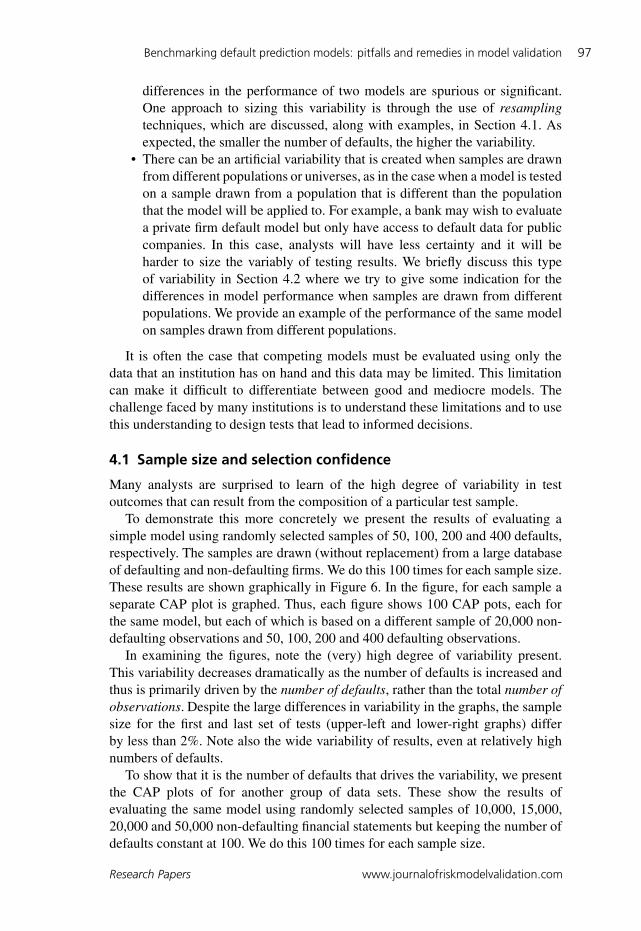
To demonstrate this more concretely we present the results of evaluating asimple model using randomly selected samples of 50, 100, 200 and 400 defaults,respectively. The samples are drawn (without replacement) from a large databaseof defaulting and non-defaulting firms. We do this 100 times for each sample size.These results are shown graphically in Figure 6. In the figure, for each sample aseparate CAP plot is graphed. Thus, each figure shows 100 CAP pots, each forthe same model, but each of which is based on a different sample of 20,000 non-defaulting observations and 50, 100, 200 and 400 defaulting observations.

In examining the figures, note the (very) high degree of variability present.This variability decreases dramatically as the number of defaults is increased andthus is primarily driven by the number of defaults, rather than the total number ofobservations. Despite the large differences in variability in the graphs, the samplesize for the first and last set of tests (upper-left and lower-right graphs) differby less than 2%. Note also the wide variability of results, even at relatively highnumbers of defaults.

To show that it is the number of defaults that drives the variability, we presentthe CAP plots of for another group of data sets. These show the results ofevaluating the same model using randomly selected samples of 10,000, 15,000,20,000 and 50,000 non-defaulting financial statements but keeping the number ofdefaults constant at 100. We do this 100 times for each sample size.


98 R. M. Stein

FIGURE 6 Variability of test results when different numbers of defaults are usedfor evaluation. These graphs show the results of evaluating a simple model usingrandomly selected samples of varying numbers of defaults. Each figure shows100 CAP pots, each of which is based on evaluating the same model using adifferent sample of 20,000 non-defaulting observations and 50, 100, 200 and400 defaulting observations.

These results are shown graphically in Figure 7 similar to the presentationin Figure 6. In this case, it is clear that the effect increasing the number ofnon-defaulting records, even by fivefold, does not materially affect the variabilityof the results. This outcome stands in contrast to that shown in Figure 6 andsupports the observation that the key factor in reducing the variability of testresults is the number of defaults used to test a model.

We can make this intuition more precise. For example, we calculated anaccuracy ratio for each of the 100 CAP plots in each graph in Figure 7. For eachgraph we then calculated the standard deviation (and interquartile ranges) of theaccuracy ratios. The SD (and IQR) for the four cases differed only at the thirddecimal place. Further, the differences showed no consistent pattern and statisticaltests showed no significant difference in distribution.

This is not unexpected. Most of the closed-form solutions that have beensuggested for the variance of the area under the ROC curve involve terms that



FIGURE 7 Variability of test results when different numbers of non-defaults areused for evaluation. These graphs show the results of evaluating the same modelusing randomly selected samples of 10,000, 15,000, 20,000 and 50,000 non-defaulting financial statements but keeping the number of defaults constant at100. It is clear that the effect increasing the number of non-defaulting recordsdoes not appear to affect the variability of the results greatly.

scale as the inverse of the product of the number of defaults and non-defaults.The intuition here is that the addition of another defaulting firm to a samplereduces the variance by increasing the denominator by the (much larger) numberof good records, while the addition of a non-defaulting firm only increases thedenominator by the (much smaller) number of bad firms.

In the extreme, Bamber (1975) describes an analytic proof (attributed to VanDanzig (1951)) that, in the most general case, the maximum variance of the areaunder the curve is given by

A(1 − A)/D

assuming there are fewer defaults than non-defaults, where A is the area underthe curve and D is the number of defaults. Another formulation, with stricterassumptions, gives the maximum variance as

(1/3ND)[(2N + 1)A(1 − A) − (N − D)(1 − A)2]where the notation is as above and N is the number of non-default records.


100 R. M. Stein

From inspection, the maximum variance in the first case is inversely propor-tional to number of defaults only, and in the second case it is inversely proportionalto the product of the number of defaults and non-defaults, due to the first term, sowhen the number of non-defaults is large, it decreases much more quickly as thenumber of defaults is increased.

Note that it is convenient to speak in terms of the maximum variance herebecause there are many possible model–data combinations that yield a spe-cific A, each producing its own unique ROC and each with its own variance.The maximum variance is the upper bound on these variances for a given A.Upper bounds for the variance in special cases (those with different assumptions)can be derived as well. However, it is generally difficult to determine whichassumptions are met in realistic settings and therefore closed-form approaches todefining confidence intervals for A based on either variance or maximum variancederivations can lead to over- or underestimates. We discuss this below.

If the number of defaults was greater relative to the number of non-defaults, therelationship would be reversed, with non-defaults influencing the variance moredramatically. Similarly, if the number of defaults and non-defaults were abouteven, they would influence the result to approximately the same degree. In general,it is the minority class (the class with fewer observations) of a sample that willinfluence the variance most dramatically.

Most institutions face the challenge of testing models without access to a largedata set of defaults. Given such a situation, there is relatively little that can bedone to decrease the variability of the test results that they can expect from testing.A far more reasonable goal is to simply understand the variability in the samplesand use this knowledge to inform the interpretation of any results they do obtainto determine whether these are consistent with their expectations or with otherreported results.

Sometimes we wish to examine not just the area under the curve, but a varietyof metrics and a variety of potential hypotheses about these statistics. To do this,we often need a more general approach to quantifying the variability of a particulartest statistic. A common approach to sizing the variability of a particular statisticgiven an empirical sample is to use one of a variety of resampling techniques toleverage the available data and reduce the dependency on the particular sample.19

A typical resampling technique proceeds as follows. From the result set, a sub-sample is selected at random. The performance measure of interest (eg, A or thenumber of correct predictions for a specified cutoff, or other performance statisticsof interest) is calculated for this sub-sample and recorded. Another sub-sampleis then drawn and the process is repeated. This continues for many repetitionsuntil a distribution of the performance measure is established. The samplingdistribution is used to calculate statistics of interest (standard error, percentilesof the distribution, etc).

19The bootstrap (eg, Efron and Tibshirani (1993)), randomization testing and cross-validation(eg, Sprent (1998)) are all examples of resampling tests.



Under some fairly general assumptions, these techniques can recover estimatesof the underlying variability of the overall population from the variability of thesample.

For example, Figure 8 shows the results of two separate experiments. In thefirst, we took 1,000 samples from a data set of defaulted and non-defaulted firms.We structured each set to contain 20,000 non-defaulted observations and 100defaulted observations. Conceptually, we tested the model using 1,000 differentdata sets to assess the distribution of accuracy ratios. This distribution is shown inthe top graph of Figure 8. In the second experiment, we took a single sample of100 defaults and 20,000 non-defaults and bootstrapped this data set (sampled withreplacement from the single data set) 1,000 times and again plotted the distributionof accuracy ratios. The results are shown in the bottom graph (adjusted to a meanof zero to facilitate direct comparison20).

Of interest here is whether we are able to approximate the variability of the1,000 different data sets from the full universe by looking at the variability of asingle data set from that universe, resampled 1,000 times. In this case, the resultsare encouraging. It turns out that the quantiles of the distribution of the bootstrapsample slightly overestimate the variability,21 but give a fairly good approximationto the variability.

This is useful because in most settings we would only have the bottom frameof this figure and would be trying to approximate the distribution in the top frame.For example, given the estimated variability of this particular sample, we candetermine that the 90% confidence interval spans about 14 points of AR, whichis very wide.

Resampling approaches provide two related benefits. First, they give a moreaccurate estimate of the variability around the actual reported model performance.Second, because of typically low numbers of defaults, resampling approachesdecrease the likelihood that individual defaults (or non-defaults) will overlyinfluence a particular model’s chances of being ranked higher or lower thananother model. For example, if model A and model B were otherwise identicalin performance, but model B by chance predicted a default where none actuallyoccurred on company XYZ, we might be tempted to consider model B as inferiorto model A. However, a resampling technique would likely show that the modelswere really not significantly different in performance, given the sample.

This example worked out particularly well because the sample we chose tobootstrap was drawn at random from the full population. Importantly, in cases

20We need to do this since the mean of the bootstrap sample will approach the value of the ARfor the original single sample, but the mean of the 1,000 individual samples drawn from the fullpopulation will approach the mean of the overall population. Due to the sampling variabilitythese may not be the same.21See Efron and Tibshirani (1993) for a discussion of adjustments to non-parametric andparametric estimates of confidence intervals that correct for sample bias, etc. Note that undermost analytic formulations, the variance of the estimate of the area under the ROC is itselfaffected by the value of the area. As a result, some of the discrepancy here may also be due tothe difference in the level of the AR, which is related to the area under the curve.


102 R. M. Stein

FIGURE 8 Two similar distributions of ARs: 1,000 samples and a bootstrapdistribution for a single sample. The top frame shows the distribution of accuracyratios for 1,000 samples from a data set of defaulted and non-defaultedfirms. Each set contains 20,000 non-defaulted observations and 100 defaultedobservations. The bottom frame shows the distribution of accuracy ratios for1,000 bootstrap replications of a single sample of 100 defaults and 20,000 non-defaults. Results are adjusted to a mean of zero to facilitate direct comparison.

-0.15 -0.10 -0.05 0.0 0.05 0.10 0.15

050

100

150

200

AR - mean(AR)

-0.15 -0.10 -0.05 0.0 0.05 0.10 0.15

050

100

150

200

AR - mean(AR)

Distribution around mean AR of 1,000 data sets: Ngood=20,000, Ndef=100

Distribution around mean AR of 1,000 boostrap replications: Ngood=20,000, Ndef=100

where a particular sample may not be drawn at random from the population, wherethere may be some selection bias, resampling techniques are less able to recoverthe true population variability. In such cases, resampling can still be used to sizethe variability of a set of models’ performance on that sample, and as such canbe useful in comparing models, but the results of that testing cannot easily beextended to the overall population.

For comparisons between competing models, more involved resampling tech-niques can be used that take advantage of matched samples. In such a setting, it ismore natural to look at the distribution of differences between models on matchedbootstrap replications.

For example, in comparing the performance of two models we are typicallyinterested in which model performs better along some dimension. One way tounderstand this is to resample the data many times and, for each sample, calculate



the statistic for each model. The result will be two sets of matched statistics, oneset containing all of the statistics for the first model on each resampled data set,and one set containing all of the statistics for the second model on each set. Thequestion then becomes whether one model consistently outperforms the other onmost samples.

Bamber (1975) also provides a (semi)closed-form solution for determiningthe variance of A, although this relies on assumptions of asymptotic normality.Bamber’s estimator derives from the correspondence between the area under theROC curve, A, and the Mann–Whitney statistic. A confidence bound for theMann–Whitney statistic can often be calculated directly using standard statisticalsoftware.

Engelmann et al (2003) discuss this approach and test the validity of theassumption of asymptotic normality, particularly as relates to smaller samples.The sample of defaulted firms in their experiments lead them to conclude thatthe normal approximation is generally not too misleading, particularly for large(default) samples. That said, they present evidence that as the number of defaultsdecreases, the approximations become less reliable. For (very) low numbers ofdefaults, confidence bounds can differ by several percentage points, however,such differences can be economically significant. As shown in Stein and Jordão(2003) a single percentage point of difference between two models can representan average of 0.97 bps or 2.25 bps additional profit per dollar loaned dependingon whether a bank was using a cutoff pricing approach, respectively. In 2002, fora medium sized US bank these translated into additional profit of about $2 millionand $5 million, respectively.

While smaller samples can lead to unstable estimates of model performancewhen using closed form approaches, Engleman et al (2003) show that the closedform results variance estimation approaches appear reasonably reliable.

It should be noted that a great advantage of Bamber’s (1975) closed-formconfidence bound is the relatively lower computational cost associated with calcu-lating confidence intervals based on this measure which enables fast estimation.One reasonable strategy is thus to use the approximations during early work indeveloping and testing models, but to confirm results using bootstrap in the laterphases. To the extent that these results differ greatly, more extensive analysis ofthe sample would be required.

4.2 Performance levels for different populations

In the previous section, we discussed ways in which resampling approachescan provide some indication of the sensitivity of the models being tested tothe particular sample at hand, and thus provide information that is valuable forcomparing models. However, this approach does not provide detailed informationabout how the models would perform on very different populations.

In this section, we give a brief example of how the performance observed onone set of data can be different to that observed on another set of data, if the datasets are drawn from fundamentally different populations. The goal of this section


104 R. M. Stein

is not to present strong results about the different universes that might be sampled,but rather to highlight the potential difficulties in drawing inferences about onepopulation based on testing done on another.

The example we choose comes up often in practice. We show that performancestatistics can vary widely when a model is tested on rated public companiesunrated public companies and private companies. In such cases, an analyst mightwish to understand a default model’s performance on a bank portfolio of middle-market loans, but incorrectly test that model on a sample of rated firms. Inferencesabout the future performance of the model on middle-market companies, based onan analysis of rated firms, could result in misleading conclusions.22

Earlier research has provided evidence that models fit on public or ratedcompanies may be misspecified if applied to private firms (eg, Falkenstein et al(2000)). A similar phenomenon can be observed in test results if models are testedon a different population than that on which they will be applied.

As an example, consider the CAP plot shown in Figure 9. The figure providesevidence of differences in performance statistics as the same model is applied torated, unrated and private firms, respectively.

This example serves to highlight the degree to which testing on the appropriatepopulation can affect decisions about models. It gives an indication of thesensitivity of models to different populations, particularly if the data are drawnfrom a population that is not representative of the population to which it will beapplied.

From this figure, we can see that the performance statistics generated fromtests run on one population are clearly different than those that were generatedfrom tests run on a different population.

What this implies is that it is very difficult to assess the performance of a modelon, say, private companies by testing on publicly rated firms. It would be evenmore difficult to compare two models intended for use on private firms if the testresults were generated using publicly rated firms. The reasons for these differencescould be manifold, from the design of the model to the nature of the data used todevelop it, and to the nature of the data used to test it. For these reasons, tests mustbe designed carefully. Given the differences in sample composition and samplesize, it is clearly inappropriate to compare these statistics directly with each other.In fact, it is not even clear how one would directly compare the statistics on thesethree samples.

For example, users of private firm models sometimes ask whether the modelmight perform well on public firms. This question can be answered, but it is only

22Note that this common-sense principle also shows up in some surprising settings, for example,in the rules of evidence that govern US court proceedings. In its landmark 1997 ruling, GeneralElectric versus Robert K Joiner, the United States Supreme Court upheld an appellate courtruling that the court may exclude scientific evidence when there is simply too great an analyticgap between the data and the opinion it is used to support. The Court ruled that, “The studies[offered as evidence] were so dissimilar to the facts presented. . . that it was not an abuse ofdiscretion for the District Court to have rejected the experts reliance on them.” (Opinion ofJudge Renquist, Supreme Court of the United States (1997)).



FIGURE 9 CAP plots of the same model applied to rated, unrated publicly tradedand private firms.

Model score

% d

efa

ults

0 10 20 30 40 50

0.2

0.4

0.6

0.8

1.0

Rated (AR=70.4)Unrated (AR=63.1)Private (AR=54.7)

meaningful to ask how the model performs relative to other public firm alternativeson public firms, not relative to the model’s performance on private firms, becauseno direct comparison can be made in this case. It can be particularly misleading todraw inferences about the performance of a model on one population if it is testedon a sample drawn from different model.

4.3 Extensions

Validation testing need not be limited to tests of model performance alone.Consider the evaluation of a model for use within a bank located where accountingdata is known to be of poor quality. Validation testing can be used to evaluatethe impact of this noisy accounting data on model performance by observingthe degradation in model performance as noise is added to test data and it is runthrough the model.

Figure 10, shows the results of adding random noise at various levels toaccounting data and running that data through a default model that was designedto be tolerant to noisy data. The noise levels indicate the distribution of the noise,in multiplicative terms, that is used to shock the accounting data and are plottedagainst the average accuracy ratio for the simulations at that noise level. So, for


106 R. M. Stein

FIGURE 10 The impact of noise levels in accounting data on accuracy ratios fora default model. The results of adding uncorrelated random errors to accountingdata and running that data through a default model that was designed tobe tolerant to noisy data are shown. As the noise levels increase the modelperformance degrades, but it does so gradually. The noise levels on the x-axisindicate the distribution of the noise, in multiplicative terms, that is used to shockthe accounting data and are plotted against the average accuracy ratio for thesimulations at that noise level.

1.0% 10.0% 100.0%2.0% 3.0% 4.0% 6.0% 20.0% 30.0% 50.0%

Noise level (=3 sigma)

0.57

0.62

0.67

Mean A

R

example, a noise level of 30% indicates that about 99% of the time an accountingvariable will be randomly increased or decreased by between 0 and 30%.

Figure 10 shows that for this particular model, the average performancedegrades as the noise levels increase, but does this fairly gradually. The noiselevels can be fairly high before the average model’s performance begins to degradesignificantly. In a fuller experiment, this would give some confidence in therobustness of the model and could provide some guidelines for its usage.

In a different study, Stein et al (2003), used validation testing approaches todetermine which risk factors, systematic or idiosyncratic, better explain privatefirm defaults. Through a series of validation experiments, they test the predictivepower of two different modeling approaches – one that relies primarily on system-atic factors and one that relies primarily on idiosyncratic factors. By segmentingthe population along dimensions that isolate these factors, they conclude that themajority, but not all, of the risk associated with private firms is attributable toidiosyncratic risk components.



5 CONCLUSION

In this article we have discussed several strategies for testing model performance.We can test for both power and calibration and these two properties are related.As a result, we find it useful to first identify the most powerful model availableand then to calibrate this powerful model. While this calibration may be flawed,by choosing a powerful model we increase the probability that the model chosen,when calibrated, will have acceptable performance. While it is never possible tocalibrate a model to future default experience, we can attempt to simulate thisthrough appropriately designed experiments.

We have discussed a framework called walk-forward testing that allows devel-opers to test models and modeling methodologies while controlling for sampleand time dependence. Where its use is feasible, the technique reduces the chancesthat models will be overfit because it never uses data in the testing that was usedto fit model parameters. At the same time, this approach allows modelers to takefull advantage of the data by using as much of the data as possible to fit and to testthe models.

The results of model testing, whether using walk-forward tests on a newlydeveloped model or whether testing a third-party model for use within a financialinstitution, are subject to sample variability. This variability is driven more by thenumber of defaults than by the total number of observations in a data set. Smallnumbers of defaults lead to very high variability results.

In general, it is not possible to reduce this uncertainty, so often the best we cando is size and understand it. We have suggested strategies, based on both analyticand resampling techniques, that permit the recovery of information about samplevariability from the sample of data at hand. We have also provided a suggestiveexample of cases in which a model could have very different performance on a testdata set than on the population to which it was being applied if that population wasstructurally different from the test set. We have shown an example of extendingthe application of validation work beyond model comparison, as in the case oftesting for model robustness in the presence of noise.

Taken as a whole, this suggests a strategy of:

• testing models against reasonable benchmarks to understand better therelative scale of performance statistics on the data set on hand;

• taking care to ensure that the population from which the test sample is drawnis similar in its characteristics to the population on which it will be applied;

• evaluating the variability of performance results through appropriate resam-pling experiments; and

• evaluating models first with respect to power and, upon selecting the mostpowerful model, testing the calibration and perhaps recalibrating.

We feel that it is of fundamental importance to understand the behavior of themetrics being calculated, to recognize the limitations of the data used to testthem and to design experiments that provide good measures of the performance


108 R. M. Stein

of default models along the dimensions that are important for the business andresearch applications at hand.

In this paper, we have attempted to bring together material from a number ofdisparate research streams and to discuss aspects of each that can have an impacton the interpretation of benchmarking results. We have found that the approacheswe describe here, while not appropriate for all models, form an effective suite oftools for benchmarking internal and external credit models where data permits andprovide guidance on interpreting results where data is sparse.

At the time that the first draft of this paper was circulated in 2002, formal modelvalidation research was still evolving. However, as evidenced by the additionalreferences and topics discussed in this updated version of the article, the past fiveyears have enjoyed increased interest both among academics and practitioners onthe issues of validation and on the limitations of various validation approaches.These results, in addition to being of keen interest intellectually, ultimately benefitpractitioners directly. They serve to highlight the importance of conducting carefulexperiments on credit model performance and, most importantly, the economicconsequences of failing to do so.

APPENDIX A TYPE I AND TYPE II ERROR: CONVERTING CAP PLOTSINTO CONTINGENCY TABLES

A common tool for evaluating default prediction models is the use of power curvesand CAP plots which graphically show the power of various models on a set oftest data. These diagnostics are often summarized though power statistics andAccuracy Ratios.

However, for some purposes, analysts and researchers are interested in under-standing Type I and Type II error rates for specific cutoffs. With knowledge of thesample default rates, these error rates are fully described by the CAP plots. In thisappendix, we describe a methodology for inferring Type I and Type II error ratesfrom these diagnostic plots.

For reference, we repeat that the CAP plot is constructed similarly to the ROCcurve. Like a ROC curve, the CAP plot describes the percentage of defaultsexcluded by a particular model for a given cutoff criteria on the y-axis. UnlikeROC curves, CAP plots display the percentage of the entire sample excluded by acutoff criteria on the x-axis (as opposed to only showing the non-defaulting creditson the x-axis, as in the ROC curve).

Thus, the x and y coordinates display the percentage of the sample excludedand the true positive rate respectively, as shown in Figure A.1.

With knowledge of the sample default rate, there is a straightforward transfor-mation that can be used to construct a table of Type I and Type II errors (andfalse negative and false positive results) from the CAP plot for any cutoff criteriaof interest. This, in turn, permits an analyst to determine what percentage of aportfolio would need to be excluded in order to capture a desired percentageof defaults or, conversely, determine the percentage of defaults that would beexcluded for a given exclusion of a portfolio.



FIGURE A.1 A schematic representation of a CAP plot.

TP%

S%

Portfolio ordered by model score percentile

Pct.

defaults

0 20 40 60 80 100k

0.0

0.2

0.4

0.6

0.8

1.0

To derive the transformation, first note that the true positive and false positiverates are defined directly from the y-axis of the CAP plot. The true negative andtrue positive rates are not directly observable from the x-axis, owing to the factthat the x-axis of a CAP plot contains both non-defaulted and defaulted firms: theentire sample (S%(k)).

As we are interested in percentages in terms of the total number of non-defaults,rather than the percentage of all firms in the sample, we need to back out thedefaulted firms. To do this, we need to know how many of them are contained inthe region between zero and the cutoff, k.

This is just the true positive rate times the total default rate, r%, since TP%(k)of the total defaults were excluded and r% of the total sample represents the totalpercentage of the sample that defaulted. This quantity,

S%(k) − (TP%(k) ∗ r%)

gives the total proportion of the entire sample that were non-defaulters, below thecutoff.

Finally, the above expression is still given in units of the total sample, ratherthan in units of the non-defaulters only. For true and false negatives, becausewe are interested in the proportion of the non-defaulters that are excluded for aparticular cutoff criterion, rather than the proportion of the total sample, we need


110 R. M. Stein

to normalize the expression above to put it in terms of total non-defaults only. Todo this, we adjust the above percentage so that it is a percentage not of the totalsample, but of the total sample minus the defaulters, or 1 − r%. This yields thefollowing expression for false positives:

FP% = S%(k) − (TP%(k) ∗ r%)

1 − r%

The remaining terms can be calculated directly.A contingency table, incorporating the above transformation, is shown in the

following table.

Actual default Actual non-default

Predicted default TP%(k)S%(k) − (TP%(k)∗r%)

1 − r%

Predicted non-default 1 − TP%(k) 1 − S%(k) − (TP%(k)∗r%)

1 − r%

In this table, k is a specific cutoff criterion, TP%(k) is the true positiverate (y-axis: percentage defaults captured) associated with criterion k, S%(k) isthe percentage of the full sample (x-axis: percentage of sample excluded) withcriterion k and r% is the sample default rate.

APPENDIX B THE LIKELIHOOD FOR THE GENERAL CASE OF ADEFAULT MODEL

In the case of a model predicting a binary event (default/no default), the model’sestimate of the probability of a single event y happening given data x is

prob(y | x) = p(x)y[1 − p(x)](1−y)

where p(x) is the probability (of default) predicted by the model, conditional onthe input x, and the event y is defined as follows:

y ={

1 if the firm defaults

0 if the firm remains solvent

Note that as either y or (1 − y) will always be 0, this reduces to the simplepredicted probability of the outcome, according to the model, conditioned on x.

For a given set of data, the likelihood of the model, L(model), is calculated bycomputing the model’s predicted probabilities, given the data inputs to the model,and calculating the appropriateness of these predictions for each observation,given the actual outcomes. Here we assume that the model is evaluated usinga specific data set and that the likelihood is thus with respect to this data set.

To do this we generalize the above probability by taking advantage of the factthat the overall likelihood of a model for a pooled data set is the product of the



individual likelihoods of any disjoint subsets of the data:

L(model) =n∏

i=1

prob(yi | xi) =n∏

i=1

p(xi)yi (1 − p(xi))

(1−yi)

In general, it is easier to work with summations than products, particularly formore complicated likelihood functions, so by convention we work with the logof the likelihood, �(model). This is also convenient computationally because forlarge datasets and small probabilities, the likelihoods can become tiny in their rawform causing underflows. The log likelihood is23

�(model) =n∑1

yi ln[p(xi)] + (1 − yi) ln[1 − p(xi)]

REFERENCES

Bamber, D. (1975). The area above the ordinal dominance graph and the area belowthe receiver operating characteristic graph. Journal of Mathematical Psychology 12,381–417.

Bell, R. M., and Cover, T. M. (1980). Competitive optimality of logarithmic investment.Mathematics of Operations Research 5(2), 161–166.

Bohn, J. R., Crosbie, P., and Stein, R. M. (2007). Active Credit Portfolio Management inPractice. Wiley, New York (forthcoming).

Blöchlinger, A., and Leippold, M. (2006). Economic benefit of powerful credit scoring.Journal of Banking and Finance 30(3), 851–873.

Burnham, K. P., and Anderson, D. R. (1998). Model Selection and Inference. Springer: NewYork.

Cantor, R., and Mann, C. (2003). Measuring the performance of Moody’s corporate bondratings. Moody’s Special Comment, Moody’s Investors Service, New York.

Dhar, V., and Stein, R. (1998). Finding robust and usable models with data mining:examples from finance. PCAI, December.

Dwyer, D., and Stein, R. (2005). Moody’s KMV RiskCalcTM 3.1. Technical Document,Moody’s KMV.

Edwards, A. W. F. (1992). Likelihood. Johns Hopkins University Press, London.

Efron, B., and Tibshirani, R. J. (1993). An Introduction to the Bootstrap (Monographs onStatistics and Applied Probability, No. 57). Chapman and Hall/CRC Press.

Engelmann, B., Hayden, E., and Tasche, D. (2003). Testing rating accuracy. RISK, January.

Falkenstein, E., Boral, A., and Carty, L. V. (2000). RiskCalc for private companies: Moody’sdefault model. Special Comment, Moody’s Investors Service.

Friedman, C., and Cangemi, R. (2001). Selecting and evaluating credit risk models. ERiskiConference series.

23Note that because yi is always either zero or one, this can also be written as ln[yip(xi ) +(1 − yi)(1 − p(xi ))] which is computationally slightly more convenient.


112 R. M. Stein

Green, D. M., and Swets, J. A. (1966). Signal Detection Theory and Psychophysics.Peninsula Publishing, Los Altos, CA.

Greene, W. (2000). Econometric Analysis. Prentice Hall, Upper Saddle River, NJ.

Gupton, G. M., and Stein, R. M. (2002). LossCalc(TM): Moody’s model for predicting LossGiven Default (LGD). Moody’s Rating Methodology. Moody’s Investors Service, NewYork.

Hanley, A., and McNeil, B. (1982). The meaning and use of the area under a ReceiverOperating Characteristics (ROC) curve. Diagnostic Radiology, 143(1), 29–36.

Hanley, J. A. (1989). Receiver Operating Characteristic (ROC) methodology: the state ofthe art. Critical Reviews in Diagnostic Imaging 29(3), 307–335.

Kelly, J. L. Jr. (1956). A new interpretation of information rate. The Bell System TechnicalJournal 35, 185–189.

Mensah, Y. M. (1984). An examination of the stationarity of multivariate bankruptcyprediction models: a methodological study. Journal of Accounting Research 22(1),380–395.

Pepe, M. S. (2002). Receiver operating characteristic methodology. Statistics in the 21stCentury, Raftery, E. A., Tanner, M. A. and Wells, M. T. (eds). Chapman and Hall/CRCPress.

Provost, F., and Fawcett, T. (2001). Robust classification for imprecise environments.Machine Learning 42, 203–231.

Reid, N. (2002). Likelihood. Statistics in the 21st Century, Raftery, E. A., Tanner, M. A., andWells, M. T. (eds). Chapman and Hall/CRC Press.

Royall, R. (1997). Statistical Evidence: A Likelihood Paradigm (Monographs on Statisticsand Applied Probability, Vol. 71). Chapman & Hall/CRC Press.

Sobehart, J. R., Keenan, S. C., and Stein, R. M. (2000). Benchmarking quantitative defaultrisk models: a validation methodology. Moody’s Special Comment, Moody’s InvestorsService.

Sprent, P. (1998). Data Driven Statistical Methods. Chapman & Hall, London.

Stein, R. M. (1999). An almost assumption free methodology for evaluating financialtrading models using large scale simulation with applications to risk control. WorkingPaper, Stern School of Business, New York University, New York.

Stein, R. M. (2002). Benchmarking default prediction models: pitfalls and remedies inmodel validation. Technical Report #020305, Moody’s KMV, New York.

Stein, R. M., Kocagil, A. E., Bohn, J., and Akhavein, J. (2003). Systematic and idiosyncraticrisk in middle-market default prediction: a study of the performance of the RiskCalc™and PFM™ models. Technical Report, Moody’s KMV, New York.

Stein, R. M., and Jordão, F. (2003). What is a more powerful model worth? TechnicalReport #030124, Moody’s KMV, New York.

Stein, R. M. (2005). The relationship between default prediction and lending profits:integrating ROC analysis and loan pricing. Journal of Banking and Finance 29,1213–1236.



Stein, R. M. (2006). Are the probabilities right? Dependent defaults and the numberof observations required to test for default rate accuracy. Journal of InvestmentManagement 4(2), 61–71.

Supreme Court of the United States (1997). General Electric Company, et al, Robert K.Joiner et ux.

Swets, J. A. (1988). Measuring the accuracy of diagnostic systems. Science 240,1285–1293.

Swets, J. A. (1996). Signal Detection Theory and ROC Analysis in Psychology andDiagnostics. Laurence Erlbaum Associates, Mahwah, NJ.

Van Danzig, D. (1951). On the consistency and power of Wilcoxon’s two sample test.Koninklijike Nederlanse Akademie van Wetenschappen, Proceedings, Series A 54.


benchmarking default prediction models: pitfalls - roger m stein

Documents