ABSTRACT

Title of Document: ABORT TRAJECTORIES FOR MANNED

LUNAR MISSIONS

E. David Beksinski Jr.

Master of Science, 2007 Directed By: Professor Mark J. Lewis

Department of Aerospace Engineering

With NASA’s renewed focus towards a permanent human presence on

the moon, comes the development of the Crew Exploration Vehicle. Unforeseen

circumstances can induce emergency situations necessitating contingency plans

to ensure crew safety. It is therefore desirable to define the feasibility of a direct

abort from an outbound translunar trajectory. Thus an astrodynamic model for

lunar transfer has been developed to allow for characterization of the abort

feasibility envelope for conceivable transfer orbits. In addition the model allows

for several trade studies involving differently executed abort options, factoring in

fuel margins. Two optimization schemes were utilized; one to expedite return

via any fuel in excess of that required for the abort, and one to explore the

boundary region of direct abort infeasibility envelope searching for plausible

abort trajectories.

The characterization and optimization of translunar abort trajectories for

the Crew Exploration Vehicle can ensure increased crew survivability in

emergency situations.

ABORT TRAJECTORIES FOR MANNED LUNAR MISSIONS

By

E. David Beksinski Jr.

Thesis submitted to the Faculty of the Graduate School of the University of Maryland, College Park, in partial fulfillment

of the requirements for the degree of Master of Science

2007 Advisory Committee: Professor Mark J. Lewis, Chair Professor Darryll J. Pines Professor Roberto Celi

© Copyright by E. David Beksinski Jr.

2007

ii

Dedication

To my parents and family whose love and support has given me so much

more then I ever thought possible. Thank you for everything Mom and Dad.

iii

Acknowledgements

I would like to express my most sincere appreciation and thanks to

Dr. Mark J. Lewis whose support and guidance has led me through my

undergraduate and into my graduate program. Also to Dr. Ryan P. Starkey for

his assistance and guidance throughout my graduate program. My gratitude

goes out to all of the professors who have led me through my journey at the

University of Maryland. And to my officemates Adam, Chris and Josh whose

guidance and company made my cubicle an enjoyable place to work, instead of,

well, just a cube. And lastly to my friends for the support and companionship

that has come to define my impressions and memories of college life.

iv

Table of Contents Dedication ..................................................................................................................ii Acknowledgements.................................................................................................iii Table of Contents.....................................................................................................iv List of Tables.............................................................................................................vi List of Figures ..........................................................................................................vii Nomenclature............................................................................................................ ix Acronyms................................................................................................................... xi Chapter 1. Introduction........................................................................................ 1

1.1. Motivation................................................................................................... 1 1.2. Research Objectives ................................................................................... 6 1.3. Thesis Overview......................................................................................... 7 1.4. Previous Lunar Abort Work ..................................................................... 7

Chapter 2. Abort Methodology ........................................................................ 15 2.1. Abort Rationale ........................................................................................ 15

2.1.1. Mechanical Failures ......................................................................... 15 2.1.2. Environmental Conditions ............................................................. 16 2.1.3. Unanticipated Hazards ................................................................... 18

2.2. Mission Overview.................................................................................... 19 2.3. Baseline Case: Apollo Mass/Propulsion Data ...................................... 21 2.4. CEV Mass/Propulsion Data .................................................................... 22 2.5. Abort Staging Methods ........................................................................... 23

2.5.1. Nominal Abort.................................................................................. 24 2.5.2. Ideal Abort ........................................................................................ 26 2.5.3. Lifeboat Case 1 Abort ...................................................................... 28 2.5.4. Lifeboat Case 2 Abort ...................................................................... 30

Chapter 3. Astrodynamic Model Development............................................ 31 3.1. Algorithm Overview ............................................................................... 31 3.2. Trajectory Characterization .................................................................... 36 3.3. Direct Abort Required ∆V....................................................................... 43

Chapter 4. Optimization of Return Trajectories........................................... 46 4.1. Expedited Return in Feasible Region .................................................... 46

4.1.1. Methodology/Algorithm ................................................................. 47 4.1.2. Implementation ................................................................................ 48

4.2. Infeasible Region Trajectory Search ...................................................... 51 4.2.1. Methodology/Algorithm ................................................................. 52

v

4.2.2. Implementation ................................................................................ 54 Chapter 5. Translunar Trajectory Analysis.................................................... 60

5.1. Reference Translunar Trajectory............................................................ 60 5.2. Translunar Abort Feasibility .................................................................. 63

5.2.1. Apollo Spacecraft ............................................................................. 63 5.2.2. CEV Spacecraft ................................................................................. 69 5.2.3. Model Verification ........................................................................... 75 5.2.4. Direct Comparison of CEV and Apollo Abort Capabilities....... 78

5.3. Abort Feasibility Across the Range of Possible Translunar Trajectories ............................................................................................................ 82 5.4. Expedited Return During Feasible Direct Aborts............................... 87 5.5. Return During Infeasible Region, Pseudo-Direct Aborts................... 94

Chapter 6. Conclusions and Implications.................................................... 100 6.1. Flexibility of Abort Trajectory Study .................................................. 100 6.2. Practicality & Conclusions for the CEV .............................................. 102 6.3. Future Work ............................................................................................ 110

Bibliography .......................................................................................................... 112

vi

List of Tables Table 2.1 Apollo spacecraft mass and propulsion data ...................................... 22 Table 2.2 CEV spacecraft mass and propulsion data .......................................... 23 Table 2.3 Nominal abort method ........................................................................... 25 Table 2.4 Ideal abort method.................................................................................. 27 Table 2.5 Lifeboat case 1 abort method................................................................. 29 Table 2.6 Lifeboat case 2 abort method................................................................. 30 Table 4.1 Direct abort fast return optimization design variables ...................... 50 Table 4.2 Pseudo-direct abort optimization design variables ........................... 58 Table 5.1 NASA historical translunar injection flight data ................................ 62 Table 5.2 Apollo abort methods infeasibility region data .................................. 68 Table 5.3 CEV abort methods infeasibility region data ...................................... 73 Table 5.4 Comparison of calculated ∆V requirements........................................ 77 Table 5.5 Upper/Lower energy trajectory bounded infeasibility regoins........ 81 Table 5.6 Pseudo-direct abort trajectories............................................................. 97 Table 6.1 Specific module fuel margin sensitivity on abort infeasibility ....... 103 Table 6.2 Specific module negative margin sensitivity on abort infeasibility105

vii

List of Figures

Figure 1.1 Representative lunar mission profile.................................................... 5 Figure 1.2 Hybrid translunar trajectories ............................................................. 11 Figure 2.1 Abort methods legend .......................................................................... 24 Figure 3.1 Direct abort trajectory ........................................................................... 33 Figure 3.2 Transit time versus translunar injection velocity.............................. 37 Figure 3.3 Required ∆V maneuvers for direct abort ........................................... 44 Figure 4.1 Constraints on flight path angle forming re-entry corridor ............ 49 Figure 4.2 Dual burn pseudo direct abort versus direct abort .......................... 53 Figure 5.1 Apollo XV feasibility profile for nominal abort (altitude)............... 63 Figure 5.2 Apollo XV First Feasibility Region...................................................... 64 Figure 5.3 Feasibility profile for Apollo XV nominal abort (time).................... 65 Figure 5.4 Feasibility profiles for various abort methods for Apollo XV ........ 67 Figure 5.5 Feasibility profile for CEV nominal abort (altitude) ........................ 69 Figure 5.6 CEV first feasibility region ................................................................... 70 Figure 5.7 Feasibility profile for CEV nominal abort (time) .............................. 71 Figure 5.8 Feasibility profiles for various abort methods for the CEV ............ 72 Figure 5.9 Abort feasibility trajectory schematic ................................................. 73 Figure 5.10 Apollo and CEV effective ∆V capabilities........................................ 79 Figure 5.11 Apollo and CEV infeasibility regions............................................... 80 Figure 5.12 Abort infeasibility versus translunar injection velocity ................. 83 Figure 5.13 Percent of mission abort infeasibility versus translunar injection

velocity............................................................................................................... 84 Figure 5.14 Abort infeasibility versus translunar injection velocity for ideal

abort in the CEV ............................................................................................... 85 Figure 5.15 Percent of mission abort infeasibility versus TLI velocity for ideal

abort in the CEV ............................................................................................... 86 Figure 5.16 Apollo XV division of ∆V high energy return................................. 89 Figure 5.17 Apollo XV nominal abort, higher energy trajectory reduction in

return time......................................................................................................... 90 Figure 5.18 CEV division of ∆V high energy return ........................................... 92 Figure 5.19 CEV ideal abort, higher energy trajectory reduction in return time

............................................................................................................................. 93 Figure 5.20 Reduction in return time for ideal CEV abort as a function of

mission time of abort initiation ...................................................................... 93

viii

Figure 5.21 CEV ideal abort, example data point locations............................... 96 Figure 6.1 Impact of fuel margin on available ∆V ............................................. 105 Figure 6.2 Percent fuel margin from added fuel mass on a specific module 106

ix

Nomenclature

ε Specific Mechanical Energy [km2/s2]

φ Flight Path Angle [deg]

µ Gravitational Constant [km3/s2]

ν True Anomaly

a Semi-Major Axis [km]

ax Acceleration X-direction [km/ss]

ay Acceleration Y-direction [km/ss]

c Foci Displacement [km]

e Eccentricity

h Angular Momentum [km2/s]

p Semi-Latus Rectum [km]

r Radius (Magnitude of radius vector) [km]

ra Apoapsis Radius [km]

rp Periapsis Radius [km]

E Eccentric Anomaly

M Mass [kg]

T Time of Flight [s]

V Velocity [km/s]

x

∆V Delta Velocity [km/s]

Vx Velocity X-direction [km/s]

Vy Velocity Y-direction [km/s]

X X Position [km]

Y Y Position [km]

xi

Acronyms

AS Ascent Stage

CEV Crew Exploration Vehicle

CM Command Module

CSM Command/Service Modules (docked configuration)

DS Descent Stage

EDS Earth Departure Stage

FRT Free Return Trajectory

GNC Guidance, Navigation, & Control

LEO Low Earth Orbit

LLO Low Lunar Orbit

LOI Lunar Orbit Insertion

LSAM Lunar Surface Access Module

LA Lunar Ascent

LD Lunar Descent

LV Launch Vehicle

RFP Request For Proposal

RCS Reaction Control System

SM Service Module

TDRS Tracking and Data Relay Satellite

xii

TEI Trans-Earth Injection

TLI Trans-Lunar Injection

1

Chapter 1. Introduction

This chapter explains the motivation for this study as well as outlines the

general format and goals of the study. A review of past abort trajectory work for

the Apollo program is included in the final section.

1.1. Motivation

The current goal set forth by NASA is to conduct a manned lunar mission

in 2018.1 Initial plans are superficially similar to the Apollo program, though

with exceptions of larger crew and increased lunar surface mission duration.

Safety will certainly be an issue for any lunar mission, and while significant

measures are taken to mitigate risk to the crew, sending people 378,000 km above

the surface of the Earth and landing them on the Moon carries an inherent risk.

Although mission planning will be performed to excruciating detail, the fact

remains that it can only account for any foreseeable circumstance. Even with

system redundancy and designing for zero single point modes of failure,

problems may arise requiring rapid return to Earth. The Apollo spacecraft had

limited transit abort capability; it is a reasonable goal that any future lunar transit

mission should be able to be performed with greater efficiency, and most

importantly, a greater margin of safety.

2

The need for contingency plan s in case of an emergency in transit to the

moon is most blatantly illustrated by the case of the Apollo XIII mission.

Mechanical failure of a fan in one of the oxygen tanks sparked and caused a

massive system failure and subsequent explosion. This induced an emergency

situation which was mitigated by conservation of available power and life

support resources and also via use of the Free Return Trajectory (FRT). Every

Apollo mission, as well as presumably any future missions, have or will utilize a

FRT or hybrid trajectory limited by FRT abort constraints. A FRT lunar transfer

is characterized by its zero delta velocity (∆V) requirements for return to Earth.

Once the Trans-Lunar Injection (TLI) burn is initiated in Low Earth Orbit (LEO),

if no other control burns are conducted, the spacecraft will slingshot around the

Moon and return to proper re-entry interface. This subset of lunar trajectories is

utilized such that in the event of an engine failure or other type of emergency,

the spacecraft will still return to Earth. Whereas, with a non-FRT, without a

decelerating burn in proximity to the moon, the spacecraft could fly past the

moon and move beyond a point of possible return. Hence the motivation for

utilization of a FRT for any manned mission is readily apparent.

The exception to this rule is hybrid trajectories, where the FRT is departed

from during the initial translunar trajectory by a midcourse correction, in order

to gain a fuel advantage allowing more expansive lunar access. While the hybrid

trajectories can allow a fuel savings, it is not done so at the cost of safety. The

3

hybrid trajectories are bounded by the abort capabilities of the spacecraft, such

that if a main engine failure occurred, an abort procedure could be performed

which would place the spacecraft on a direct return to a re-entry trajectory. The

application of these hybrid trajectories would therefore be highly dependant on a

well defined design space of abort trajectory options and spacecraft capabilities.

Motivation for a study of abort feasibility and optimized return is readily

apparent in the Crew Exploration Vehicle (CEV) Technical Requirements, as

explained in the Request For Proposal (RFP) released by NASA. The following

three requirements directly quoted from the RFP Section 6.0 CEV Technical

Requirements2 pertain directly to the need for this research:

Req. #2. Provide an abort capability during all phases of flight.

Req. #10. Be capable of return from lunar orbit to the earth surface

without assistance from external Constellation elements.

Req. #12. Abort capability independent of Launch Vehicle (LV) or

Earth Departure Stage (EDS) flight control.

With reference to requirement number two, abort capability could imply

use of FRT or direct abort; as it will be shown that ∆V cost requirements for

certain mission phases are prohibitively high. Requirement number ten seems to

imply that the CEV must have a ∆V budget sufficient to return to Earth without

refueling or any other required support from lunar based assets. Lastly

requirement number twelve indicates the CEV must have an abort capability

4

independent of LV and EDS stages. The EDS stage is the stage that provides the

TLI burn initiating the lunar transfer orbit. As will be discussed, this sets the

basis for the CEV ∆V budget based on the assumption that the LV and EDS will

not be required or available for utilization by the CEV for the remainder of the

lunar mission. In addition, upon completion of the TLI burn, the large ∆V

maneuver has already been imparted upon the spacecraft to attain lunar orbit

altitude. The spacecraft subsequent to the TLI maneuver will have high velocity

and the EDS propulsion system will be depleted, thus negating any possible gain

from its use during an abort. Figure 1.1 shows the representative Apollo mission

profile, which was used as a baseline for this analysis of future missions.

5

Figure 1.1 Representative lunar mission profile

While the possibility for an emergency situation arising from any single

mechanical, environmental or health concerns is slight; failures of these types

occur routinely on manned spacecraft. Although contingencies for these

concerns can be planned for, it is namely the concerns which have not been

thought of that preclude the necessity for sound and reliable mission abort

scenarios.

6

1.2. Research Objectives

The primary research objective is naturally to specifically characterize the

feasibility of a direct abort at any time during lunar transit. The characterization

will form a direct abort feasibility profile from which abort feasibility can be

determined quickly by inspection across the duration of the translunar trajectory.

A secondary research objective is based upon the abort feasibility profile.

It is reasonable to presume that as the ∆V requirement for direct abort varies,

during segments of the translunar trajectory when a direct abort is feasible, the

amount of ∆V available can exceed the direct abort requirement. Therefore the

goal of optimal usage of any excess fuel to attain a higher energy return

trajectory would be beneficial to crew survivability via reduction of time of flight

to re-entry.

Once the direct abort feasibility has been characterized and higher

energy trajectory options have been explored, a final research objective is to

survey the trajectory design space for other possible options. A similar

optimization scheme to the secondary research objective is used to explore

the boundary of the infeasibility region. An effort to find any possible return

trajectories utilizing multiple trajectory segments could offer further options

for the crew in an abort scenario.

7

1.3. Thesis Overview

Chapter 1 covers and introduction to the problem and a review of

previous abort studies conducted for the Apollo missions. A detailed rationale

for direct aborts as well as spacecraft overview is given in Chapter 2. Also

included in Chapter 2 is the development of four different abort staging

strategies and their impact on available ∆V for the spacecraft. Chapter 3 outlines

the development of the astrodynamic model utilized for the abort feasibility

study. Chapter 4 explains the two different optimizations utilized; one to

achieve a faster return time via utilization of any fuel left after a direct abort, and

a second to search the abort trajectory design space for trajectories consisting of

multiple course corrections. A typical translunar trajectory is thoroughly

analyzed and explained in Chapter 5. Lastly, Chapter 6 outlines the impacts of

this study on future manned lunar missions.

1.4. Previous Lunar Abort Work

Unmanned lunar bound spacecraft such as the Lunar Prospector mission

launched in January of 1998 can offer some insight along similar trajectories to

those used for Apollo and soon the CEV. The Lunar Prospector utilized a

trajectory characterized by a 105 hour time of flight; a lesser degree of orbital

transfer energy than the approximately 72 hour transit times for Apollo.3

8

Important facts that can be taken from this mission for abort scenarios

include the use of NASA Tracking and Data Relay Satellite (TDRS) for accurate

real time telemetry information. Accurate telemetry data combined with three

trajectory correction maneuvers allowed mission controllers to place the

spacecraft within 10 miles of its targeted lunar orbit altitude and within .1

degrees of the target inclination. Use of telemetry data from the TDRS confirmed

engine burn ∆V maneuvers were within 1% of targeted values. 3 The

conglomeration of this information has a positive impact on the outlook for

future lunar mission abort scenarios. Given the accurate telemetry data

available, as well as engine performance metrics, it can be established with

confidence that the exact location and ∆V capabilities of the CEV can be

ascertained throughout the mission. Vitally important for any abort trajectory

maneuver is an accurate knowledge of starting position and velocity, which is

crucial to ensuring safe transit into the re-entry corridor.

Previous studies of abort feasibility and trajectories are primarily centered

on the Apollo program as this is the only other program involving manned lunar

missions. As with the CEV RFP requirements, an operational constraint of the

Apollo missions stipulated that the spacecraft must be able to return the crew

safely to Earth from any point during the mission.4 Spacecraft return can be

accomplished via a combination of available abort trajectories and also

utilization of a free return trajectory. It was known that in a certain range along

9

the translunar trajectory the ∆V requirements were prohibitively high. Thus any

abort would either have to rely on the FRT to come back to Earth or wait until a

direct abort becomes feasible.

Two major classes of aborts were examined previously for Apollo;

minimum ∆V abort trajectories and minimum time of flight abort trajectories.

Minimum ∆V abort trajectories define the lowest possible ∆V requirements for

return to Earth, unbounded by constraints of landing at a predetermined

location. Landing site constraints were removed due to the added ∆V

requirement of any such landing site constraints. Minimum time of flight abort

trajectories are directly dependant on both available propulsion capabilities and

position along the translunar trajectory. 5

In an effort to increase the lunar landing site range for the Apollo

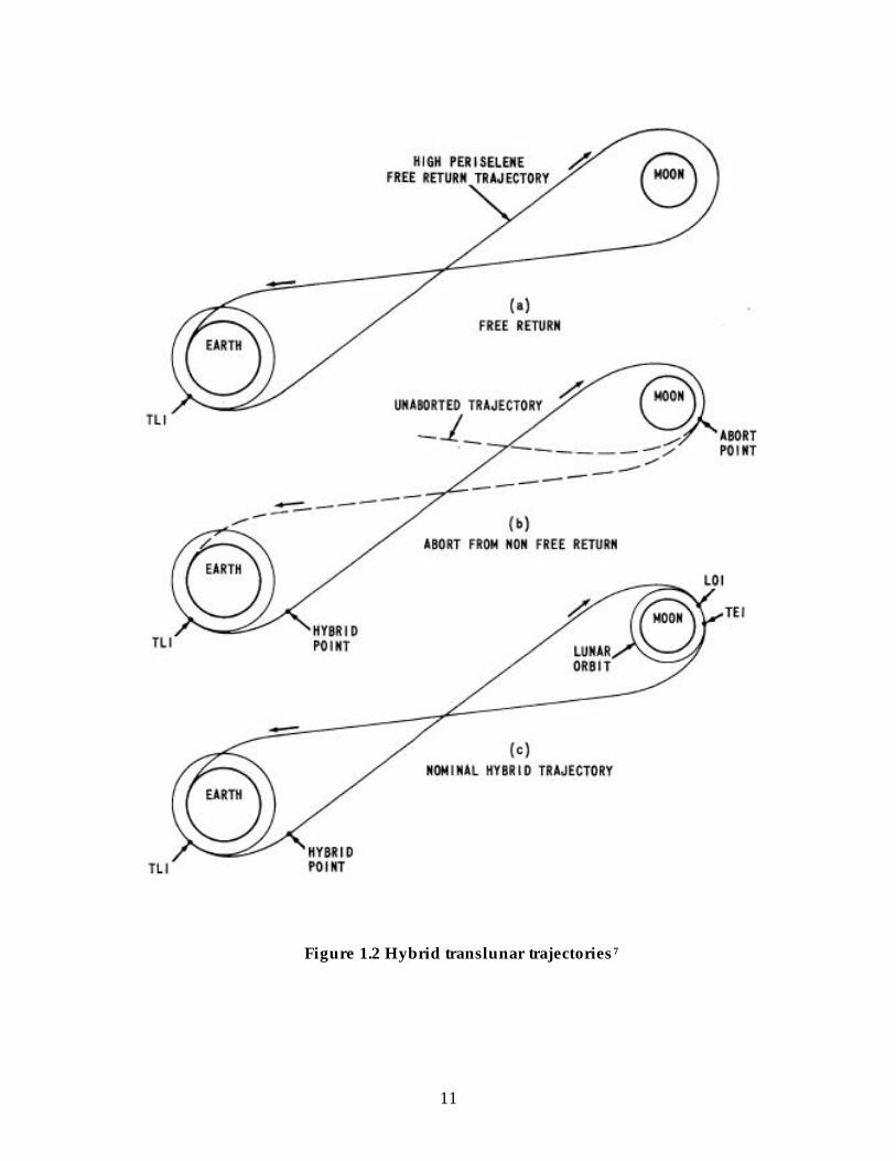
program hybrid trajectories were studied and utilized on the Apollo 14 mission.6

The hybrid trajectory allows a larger possible design space of translunar

trajectories by relaxation of the free return trajectory constraint. Hybrid

trajectories could be engaged in two ways. The first involves the injection of the

spacecraft into a TLI trajectory that satisfies the free return trajectory constraint,

followed five to ten hours later subsequent to a comprehensive propulsion and

guidance systems check, by a mid-course correction maneuver placing the

spacecraft on a non-free return trajectory. The second method involves a direct

injection at TLI into a non-free return trajectory. In relaxing the free return

10

trajectory constraint, a surrogate constraint was imposed on the mission design

criteria. All hybrid trajectories must satisfy an abort constraint based on the

lunar module descent propulsion system in the event that the service module

propulsion system failed at lunar orbit insertion.6

Optimization schemes were also previously developed by Bass in 1970 to

minimize the total ∆V for the Apollo hybrid trajectory missions. The energy

level of the hybrid trajectory was bounded on the lower range by the descent

propulsion system abort capabilities, and on the high end by the ∆V cost of a

similar mission along a free return trajectory. Optimization schemes enabled

hybrid trajectories that could reach areas of the lunar surface previously out of

the feasible mission required ∆V range for the Apollo spacecraft. An important

special case arose out of the optimization; that for landing sites far from the lunar

equator, the abort ∆V requirement always exceeded the abort capabilities. 7

The high ∆V requirement for an abort from trajectories to lunar polar

regions could influence the design of the CEV, as one of the design criteria

stipulates global lunar access. While the utilization of hybrid trajectories can

facilitate this goal; propulsion capabilities of the lunar module should be

designed to provide adequate abort capacity for global lunar access. Figure 1.2

illustrates the hybrid trajectory concept.

11

Figure 1.2 Hybrid translunar trajectories7

12

Another significant concept studied for the Apollo program involves

increasing abort capabilities of the spacecraft via jettisoning the service module.

Utilization of the lunar module descent propulsion system for abort burns could

be possible in the event of service propulsion system failure at lunar orbit

insertion. Primary reasoning for this strategy lies in reducing the spacecraft’s

mass such that the lunar module descent propulsion system has an increased

effective ∆V capability. The lunar module ascent system was not considered for

utilization due to insufficient Reaction Control System (RCS) capabilities to

control the spacecraft with the command and service module still docked.8 From

this fact an important design criterion for the CEV lunar module can be drawn.

In order to allow for maximum flexibility in off-design spacecraft configurations,

primarily extreme abort situations, the RCS system for each module should be

robust enough to control the spacecraft when at its maximum possible mass.

The “Translunar Abort Techniques for Non-Free-Return Missions”8 study

for Apollo centered on the assumption of service module propulsion failure at

lunar orbit insertion, implying that fuel tanks would be virtually full. With no

way to transfer fuel between the service module and lunar descent modules, the

service module fuel allotment becomes unutilized, dead mass. It is with this in

mind that it was recommended to jettison the service module. The reduction in

mass of the total spacecraft increased the effective ∆V of the lunar module

descent stage roughly 70% from 2700 feet per second to 4600. The increase in ∆V

13

made a single burn abort trajectory of approximately 3400 feet per second a

feasible option.8

Jettisoning the service module requires the lunar module to provide life

support for the crew during the return trajectory as the command module would

be required to shut down to conserve resources. Creating a dependency of three

crew members on a life support system designed for a crew of two implies an

added time constraint in return trajectories. Upon reaching the re-entry interface

the crew would enter the command module and jettison the lunar module for re-

entry. The principle strategy of reduction of spacecraft mass to improve effective

∆V of available propulsion systems will become central to several different abort

methods.

A final abort concept studied in the Apollo program is that of a manual

abort. In an emergency situation it is necessary to consider the ramifications of

partial or total loss of guidance and navigation. With this in mind a procedure

was developed involving a visually guided abort maneuver utilizing the docking

reticle to target Earth. In this situation the target landing site constraint has been

removed, due to emergency conditions, a fastest time to return is preferable over

landing site specification. It was found that there exists a preferred abort station

along a given translunar trajectory for manual abort. This station is defin ed by a

maximum allowable error tolerance on ∆V while maintaining safe re-entry

corridor conditions. For the standard Apollo reference trajectory this point

14

occurs approximately 31 hours after the initial translunar injection burn. At this

point an allowable ∆V dispersion of plus or minus 450 feet per second exists.9

The manual abort targeting method was partially flight verified during the

Apollo XIII mission. Although Apollo 13 utilized the free return trajectory abort

option, a midcourse correction was performed using the Earth viewed through

the docking reticle method during the return leg of the mission. While

complicated and very difficult to perform it was proven feasible.

Due to similarities in spacecraft architecture between the Apollo and CEV

design much of the previous work can be applied to the new. While differences

in the CEV design can lead to differing abort strategies, the fundamental

motivations and concepts of Apollo abort studies lay a comprehensive

foundation for any future lunar mission abort strategy.

15

Chapter 2. Abort Methodology

The motivation for a comprehensive abort trajectory study has been given

in Chapter 1, this chapter starts with an explanation of what causes could

necessitate a direct abort. Next follows an overview of a typical mission, as well

as identifying spacecraft masses and propulsive capabilities. From these masses

and ∆V capabilities, four different abort staging methods can now be developed.

2.1. Abort Rationale

2.1.1. Mechanical Failures

As with any other mechanical system, the CEV will almost certainly

encounter occasional failures. Any system is only as reliable as its least reliable

component. The complexity of the spacecraft and the environments it is

designed to operate in compound the strain on the spacecraft. Even prior to

launch the spacecraft is subjected to various physical loads during assembly and

launch preparation.

The cause of the Apollo XIII incident has been traced back to launch

preparations where the affected oxygen tank was allowed to slip and fall only a

few inches during installation. This single event caused some heater wires inside

16

the tank to loosen just enough to be exposed to oxygen, eventually leading to the

catastrophic failure of the tank and the resulting mission crisis.

Acceleration forces can impart strong loading conditions on the spacecraft

as it is propelled into orbit. Once in orbit, various environmental concerns such

as: radiation, thermal loading, space debris, and internal spacecraft

pressurization against vacuum, can all impart physical loads on the systems.

Material defects can also cause concern. Small imperfection in materials

undetectable to the eye can cause failure of mechanical components long before

their designed failure limit.

All of the above listed mechanical concerns are planned for and every

step is taken to avoid such failures via quality assurance practices and redundant

design characteristics. However it is not possible to attain total assurance against

all these issues and therefore abort scenarios for mechanical failures are

situations that must be planned for.

2.1.2. Environmental Conditions

The Earth offers protection from many environmental hazards; the

spacecraft can protect the crew to a certain degree, but cannot be a guaranteed

haven. Radiation is of key concern. While the spacecraft can offer shielding, the

sheer mass of shielding required to block all radiation is prohibitively high. The

boundary of the magnetosphere is approximately 95000 km above the surface of

17

the Earth.10 Implying that during any given manned lunar mission, the crew can

rely on the Earth’s magnetosphere for protection from solar events only for less

than the first 25% of the journey.

Compounding the radiation concern is the insufficient understanding and

prediction of solar events. The eleven year cycle of maximum solar activity is

somewhat understood, however only on a statistical basis. Virtually all

predictive solar activity models to date are based on a statistical analysis of

observation records.10 While these statistical models can form a reasonable basis

of understanding for mission planning, they are not founded on a physical

understanding of solar activity. The implication is that predicting a solar event

based on physical evidence or precursors to a solar flare is not possible, and

therefore warning time is on the order of hours. However statistically unlikely a

major solar eruption is during any given mission, the fact remains it is something

that cannot be determined far enough in advance to postpone launch. Therefore

a fastest return to Earth abort is an entirely necessary situation to avoid

potentially fatal radiation exposure.

NASA’s long term goals also have an effect on the need for abort

trajectories due to solar events. President George W. Bush 11 and NASA Director

Michael Griffin have both stressed the importance of a permanent human

presence in space and the importance of a permanently manned lunar base both

for operations in both Earth-Lunar space as well as interplanetary space to Mars

18

and beyond. A major implication of this level of space operations is a drastic

increase in manned space flight frequency over the next few decades. While

missions can be planned around statistical predictions of solar activity, and any

likely lunar base would have a radiation shielded “fallout” type shelter for solar

storms; any spacecraft in transit during a solar event will likely need to at

minimum abort to LEO for shelter. Frequent re-supply and crew transfer

missions increase the odds of an in-transit solar event necessitating a direct abort.

Another space environmental hazard is space debris and micro

meteorites. Significant effort is placed in tracking space debris and Earth-

crossing asteroids. However there is a limit on how many objects can be

tracked.12 The closing speeds of any object on a collision course with a spacecraft

makes even a fleck of paint dangerous. Impacts on the spacecraft from such

debris do occur and could potentially cause enough damage to necessitate an

abort scenario.

2.1.3. Unanticipated Hazards

The subject of unanticipated hazards is a final category that covers

anything else that could go wrong. A large concern is emergency healthcare in

space. Although astronauts endure a rigorous selection criteria, and strict health

examinations, the possibility for some unforeseen medical condition will always

be present. Medical training is mandatory for at least one member of the flight

19

crew, but limited training cannot come close to meeting the needs as a

professional doctor could. Medical equipment has advanced to assist in

emergency requirements such as portable defibrillators and pre-dosed auto

injection syringes allowing for a fairly substantial medical coverage in a

relatively small package for the spacecraft. However, in the event of an

astronaut requiring professional medical care, the spacecraft should perform the

function of an ambulance; stabilize and transport the patient to a medical facility.

In light of limited resources combined with difficulties in providing care due to

micro gravity effects, it is unreasonable to expect any transport spacecraft to offer

the medical equivalent of a trauma center. Such capabilities may one day be

realized on a larger space station, however for the present CEV and similar

vehicles, emergency medical care would prompt a direct abort scenario.

Although contingencies for any anticipated concerns can be planned for, it is

namely the concerns which have not been thought of that necessitate the need for

mission abort scenarios.

2.2. Mission Overview

A typical manned lunar mission consists of five major engine firing

events. Each propulsive maneuver initiates a primary phase of the mission.

First the Trans-Lunar Injection (TLI) maneuver is conducted. The

propulsion system responsible for this engine burn is the Earth Departure Stage

20

(EDS). Generally, as was the case for the Apollo spacecraft, the EDS is the top

stage of the launch vehicle, thus the ∆V requirement for TLI does not bear on the

spacecraft design. Once the TLI burn is completed the spacecraft coasts until the

lunar interface has been reached.

At this point the spacecraft must complete the Lunar Orbit Insertion (LOI)

maneuver. The LOI propulsive burn injects the spacecraft into a circum-lunar

orbit. The circum-lunar orbit, also known as Low Lunar Orbit (LLO) is typically

on the order of 100 km above the lunar surface and serves as the parking orbit for

the service and command modules of the spacecraft during lunar surface

excursions in the lander modules.

Once the spacecraft has achieved LLO, the next phase of the mission is

conducted by the lunar lander. The Lunar Descent (LD) mission phase is the

propulsive burden of the lunar descent module. As will be important later in

mass ratio calculations, it is important to note that the service and command

modules remain in LLO, and only the lunar module descent and ascent stages

descend to the lunar surface.

Following surface excursion activities the next phase of the mission is that

of Lunar Ascent (LA). The LA maneuver is performed by only the lunar module

ascent stage, as the descent stage is left on the surface. The crew then docks with

the command and service modules for the return trip to Earth.

21

The last mission phase is initiated by the Trans-Earth Injection (TEI)

maneuver. This engine burn imparts the spacecraft onto a coasting trajectory

directly into the re-entry interface upon return to Earth.

2.3. Baseline Case: Apollo Mass/Propulsion Data

When developing a set of abort strategies to study, it is necessary to

establish a baseline case from which to build various abort options. The Apollo

missions are the only previous example of manned lunar missions and thus an

obvious choice. At the time of development, final mass estimations for the CEV

were not yet available, thus the masses and propulsion capabilities of the Apollo

spacecraft modules formed a reasonable basis for model development. Table

2.113,14,15 shows statistics on individual modules utilized during the initial study.

It is important to note that the ∆V capabilities listed are only for the specified

module. As will be discussed later, a propulsion system’s effective ∆V when

docked with other modules is calculated via mass ratios of the docked modules.

22

Table 2.1 Apollo spacecraft mass and propulsion data

2.4. CEV Mass/Propulsion Data

In December of 2005, NASA released a report entitled “NASA’s

Exploration Systems Architecture Study (ESAS).”1 The ESAS report detailed the

recommendations for the new CEV architecture. Every conceivable system

architecture was evaluated and a final architecture was presented. It was

decided that the CEV would retain the basic module structure of Apollo,

however with some key changes. The modules would be sized for a crew of six

and designed for extended lunar surface mission durations of the entire crew.

The command and service module is to be left unmanned in low lunar orbit

during surface excursions. As shown in Table 2.21, this results in a

comparatively larger lunar module than that of Apollo. Other notable changes

include increased ∆V capability of the lunar module to afford global lunar access.

In a departure from the Apollo architecture, the service module propulsion

system is only responsible for the Trans-Earth Injection (TEI), while the Lunar

Surface Access Module (LSAM) descent stage assumes responsibility for the

23

Lunar Orbit Insertion (LOI) maneuver. Again as with the Apollo data, the ∆V

listed in Table 2.2, is the capability of each CEV module alone, different staging

options offering various effective ∆V’s for varying abort strategies will be

addressed via mass ratios.

Table 2.2 CEV spacecraft mass and propulsion data

2.5. Abort Staging Methods

Four separate abort staging methods were investigated for this study.

Since both the Apollo and CEV spacecraft have similar basic module architecture

all four methods are applicable to either spacecraft. Differences in relative

module mass fractions affect the effective ∆V for each method. The effective ∆V

available in each method is directly related to the abort capability during the

translunar trajectory. The feasibility of performing an abort maneuver increases

with increasing effective ∆V. Figure 2.1 illustrates the symbols used throughout

the descriptions of the four abort methods.

24

Figure 2.1 Abort methods legend

2.5.1. Nominal Abort

The nominal abort staging option provides a direct abort capability while

maintaining a standard mission spacecraft module configuration. In this

method, the lunar module propulsion system is utilized, first descent stage

following by descent stage jettison and burn of ascent stage engine. Next the

service module propulsion system is utilized. For the duration of the return

flight time the service module, command module and lunar ascent module

remain docked affording the maximum possible living space and, conceivably,

consumable resources. The service module and lunar ascent module would be

jettisoned just prior to re-entry as in a typical mission. This method is

25

summarized in Table 2.3. For clarity the current staged burn has been indicated

by a small flame symbol.

Table 2.3 Nominal abort method

The nominal abort configuration offers the maximum possible allotment

of resources during the abort trajectory. By retaining the lunar module ascent

stage until just prior to re-entry the habitable volume is dramatically increased.

For the Apollo spacecraft, the habitable volume of the command module is 6.17

cubic meters, while the lunar module ascent stage is 6.65 cubic meters.14,15 The

addition of the lunar ascent module more then doubles the habitable volume for

the crew during the duration of the abort trajectory. While the CEV will be

designed for a larger crew it is likely that the habitable volumetric ratio between

the CEV command module and the lunar ascent module will remain in the

approximate range of the Apollo spacecraft modular volumetric ratio. In

addition, with the design criterion of extended lunar surface excursions, it is

likely the CEV lunar module will retain a signific ant habitable volume. Tandem

to the habitable volume increase will be an inherent life support capability

26

comprised of the combined resources from the command module and lunar

ascent modules.

2.5.2. Ideal Abort

The ideal abort method summarized in Table 2.4 below is very similar to

the nominal abort. The difference is that prior to the final engine burn by the

service module the lunar ascent module is jettisoned. The lunar module jettison

is performed as a sacrifice of habitable volume and potentially usable

consumable supplies still in the lunar module in exchange for decreasing the

mass. For the Apollo spacecraft this mass advantage affords an extra kilometer

per second of effective ∆V. The effective ∆V gain for the CEV is still significant,

approximately half a kilometer per second of ∆V, however not as large as the

gains the Apollo spacecraft achieved due to the reduced size of the service

module. The service module for the CEV only performs the TEI burn, whereas

the service module for Apollo performed the LOI and TEI burns, thus the CEV

service module has comparatively less ∆V to start with, reducing the gain in

effective ∆V.

27

Table 2.4 Ideal abort method

Although the ideal abort method involves the jettisoning of the lunar

ascent module and thereby sacrifice of any available resources contained therein;

the CEV design will likely assist in mitigating any negative effects. Based on the

CEV design criterion of the service module remaining un-manned in low lunar

orbit for durations on the order of weeks to months, the service module is

designed with solar panel power supply.1 During the course of the Apollo XIII

mission abort, it was necessary to retain the lunar module for life support as well

as for power to re-start the command module guidance navigation and control

computer prior to re-entry. With the addition of solar panels, a non consumable

power supply is available to charge spacecraft batteries; contrary to the oxygen

consuming fuel cells of the Apollo spacecraft. It can reasonably be presumed

that a small amount of consumables, such as water and food could be transferred

to the command module prior to jettisoning the lunar module. This combined

with the solar power capability could help mitigate the negative drawbacks to

jettisoning the lunar module.

28

2.5.3. Lifeboat Case 1 Abort

The lifeboat case 1 abort method is the first of two methods devised to

afford the largest mass fraction advantage via module staging, as overviewed in

Table 2.5. The concept relies on utilization of the lunar module ascent stage as a

lifeboat of sorts. For the Apollo spacecraft the largest modules by mass are the

lunar module descent stage and the service module. By utilizing the available

fuel in the service module first, jettisoning it, and subsequently burning the

available fuel in the lunar module descent stage and jettisoning it as well, the last

burn by the lunar module ascent stage achieves the lightest mass ratio possible.

The Apollo spacecraft affords approximately 300 additional meters per second of

∆V in this manner. Of note for the CEV is that effective ∆V is actually less then

that of the ideal abort case. The lifeboat case methods were derived prior to the

release of the ESAS report and the subsequent mass specifications for the CEV

modules rendered the two lifeboat methods less then optimal due to the sizing

and differing propulsion responsibilities of the modules.

29

Table 2.5 Lifeboat case 1 abort method

While the loss of the service module resources imposes a serious

limitation on the life support capabilities of the spacecraft, it is potentially a

sacrifice made to gain a time advantage to return of the crew. The combined

available power of the command module with that of the lunar ascent stage

would be of key concern, as well as, the oxygen available for life support. This

extremely life support limited method would likely be utilized in situations

where the return time was on the order of 10 to 15 hours; with such short return

time of flight the primary consumable resource concern is reduced to oxygen for

breathing. Presumably, the gain in return time outweighs the need for water for

the crew during the return. The lifeboat method therefore has potential merit for

abort trajectories initiated early in the outbound translunar trajectory, though

bounded in practicality by the power and life support capabilities of the

spacecraft lunar ascent and command modules.

30

2.5.4. Lifeboat Case 2 Abort

The lifeboat case 2 abort method, illustrated in Table 2.6, is very similar to

its previous counterpart. This method simply switches the order of the first 2

stages, the lunar module descent stage and the service module. It was predicted

that this would not improve the effective ∆V for the Apollo spacecraft. However

due to ease of integration via mass ratios it was deemed worthy of examination.

Unfortunately, upon inclusion of the updated CEV mass and propulsion

capabilities it proved even less beneficial. The methods retention, if nothing else,

serves to illustrate via comparison the benefits of the other three abort methods,

reinforcing the merits of their utilization.

Table 2.6 Lifeboat case 2 abort method

Although mass ratios involved with this abort method preclude the

practicality of its utilization, the same life support constraints as the first lifeboat

abort method apply equally to this method.

31

Chapter 3. Astrodynamic Model Development

Now that spacecraft propulsive capabilities and various abort methods

have been discussed in Chapter 2; this chapter outlines the creation of an

astrodynamic model. It flows from the characterization of a translunar

trajectory, to the method of determining direct abort ∆V requirements.

3.1. Algorithm Overview

The lunar transit is the mission phase of most concern and uncertainty

during emergency situations. This is defined as the period of time after TLI burn,

but before Lunar Orbit Insertion (LOI) burn, as was shown in Figure 1.2. Aborts

performed during lunar transit are the most critical for several reasons, in

mission phase order:

1) Prior to the TLI burn in LEO an abort and subsequent re-entry will

be relatively straightforward, as the TLI energy has not yet been imparted on the

spacecraft.

2) After the LOI burn; the spacecraft is already in a low orbit around

the moon and return would simply involve pushing up the schedule of the

Trans-Earth Injection (TEI) burn which has already been planned for earth

return.

32

3) During Lunar Descent (LD); the spacecraft would use available ∆V

allotted for full LD and Lunar Ascent (LA) phases to return to Low Lunar Orbit

(LLO) and initiate TEI burn for Earth return.

4) After LA and LLO; initiate TEI burn for Earth return as presented

in cases 2) and 3) for a mission abort.

5) After the TEI burn and before Earth re-entry; as the mission has

already been completed, the only fuel that remains is the small percentage of

allowable fuel margin. The allowable fuel margin is presumably negligible;

however, it could potentially be used to increase return velocity thereby

reducing time to return, provided re-entry concerns are met.

It is for these aforementioned reasons that the scope of abort feasibility

will be focused on the outbound lunar transit mission phase.

In the event of an emergency situation requiring an abort scenario there

are two possible methods of return:

1) Do nothing; utilize the FRT which would presumably be planned

into the mission as essential to crew safety.

2) Perform a direct abort; effectively halting the spacecraft and

turning around to return to Earth, the astrodynamic equivalent of a U-turn, as

shown in Figure 3.1.

The first option of abort via free return trajectory requires little study in

regards to feasibility as it is a passive abort method requiring no trajectory

33

change maneuvers. In the case of a hybrid trajectory being utilized, as with

Apollo, the hybrid trajectory would be designed with abort capabilities as a

constraint.

Figure 3.1 Direct abort trajectory

The second method of aborting a lunar mission via direct abort is the

primary subject of the present study. In order to design for the possibility of a

direct abort, a model needs to be created to study the method feasibility and

requirements. The model should also be flexible so as to accept a wide variety of

translunar trajectories such that any future missions can be examined.

Direct solution of the basic orbital equations served as a basis for the

model rather than the patched conic method due to errors incurred in return

34

trajectory calculations. The patched conic method works well for outbound

trajectories as when the primary gravitational force of the Earth is considered,

the lunar gravitational force on the spacecraft is ignored. The magnitude of the

Earth’s gravitational force compared to the lunar gravitational force on the

spacecraft makes this assumption an acceptable one. The patched conic method

only considers the lunar gravitational force on the spacecraft when it is inside the

lunar sphere of influence, at which point the Earth’s gravitational field has a

weaker effect. Problems arise in the return trajectory however when the inverse

of the situation is utilized. When leaving lunar space, the gravitational force on

the spacecraft from the Earth’s influence compared to that of the Moon’s is not a

negligible factor. In this case the Earth’s influence is simply too large to be

ignored as in the case of ignoring the lunar gravitational influence for lunar

bound trajectories. As the focus of this study is abort trajectories returning the

spacecraft to Earth the errors incurred by utilizing the patched conic method on

return trajectories prohibited the use of the method.

In creating an astrodynamic model two primary objectives must be

addressed. First, the model must accurately track the trajectory. A translunar

trajectory, as well as any orbital trajectory, can be defined by stipulating position

and velocity. In the case of translunar trajectories, the obvious choice for

trajectory definition is the altitude and final velocity at engine shut down

following the translunar injection maneuver. From this point until injection into

35

low lunar orbit the ability to accurately determine abort feasibility is directly

dependant on the ability to track the spacecraft’s trajectory with accuracy.

The second of the primary objectives for the astrodynamic model is the

determination of abort requirements. Any abort maneuver to place the

spacecraft on a return to re-entry trajectory will have a defined ∆V requirement

based on the current position and velocity of the spacecraft. In order to

specifically define the regions of the translunar trajectory where a direct abort is

feasible the required ∆V maneuver must be known at all points in transit on the

translunar trajectory. By directly comparing the abort ∆V requirement with the

propulsive capabilities of the CEV via various staging options across the

translunar trajectory, the feasibility of a direct abort at any point during transit

can be determined.

Once the available trajectory has been defined, tracked, and abort

feasibility regions determined, a secondary objective for the astrodynamic model

emerges. While it is known that at some intermediary region during the

translunar trajectory the ∆V requirement for a direct abort will likely exceed the

propulsive capabilities of the CEV, the converse is also true. It is not

unreasonable to postulate that there will be regions where the direct abort ∆V

requirement is less then the propulsive capabilities of the spacecraft. For these

regions of direct abort feasibility it would be advantageous to ascertain the

magnitude of the fuel margin in excess of the required ∆V for direct abort. The

36

excess fuel margin subsequent to abort would serve no purpose upon arriving at

the re-entry corridor interface. Therefore it is desirable to attempt to utilize the

excess fuel to attain a higher energy return trajectory; consequently a reduction

in time of flight to return can be achieved. In an emergency situation requiring a

direct abort, it is likely that any decrease in time to return would be beneficial to

crew survivability.

3.2. Trajectory Characterization

In order to more thoroughly define the abort feasibility envelope, possible

lunar transfer orbits were modeled to provide a baseline. To characterize the

possible lunar transition orbits, the Time Of Flight (TOF) was decided upon as

the dominant metric. With the knowledge that a Hohmann transfer would have a

transit TOF of 120 hours and that this is in general the lowest possible energy

transfer, it set a bounds for the possible range.16 Thus it was decided to evaluate

the possible transfer orbits ranging from a TOF of 32 hours up to 120 hours for

future missions. The lower bound of 32 hours is based upon the required TLI

velocity to achieve such a short TOF. Not only is 11.2 kilometers per second a

potentially prohibitively high ∆V, it represents the transition of lunar trajectories

from elliptical to hyperbolic. Figure 3.2 illustrates the relationship between TLI

velocity and its consequential TOF to lunar orbit.

37

Figure 3.2 Transit time versus translunar injection velocity

Although not included in this present effort, higher energy transfers (TLI

velocity greater than 11.2 km/s to reduce TOF further) could be accounted for by

simply changing the bounds. Though it was presumed that due to the nature of

the system the vast ∆V increase required for an almost trivial reduction in TOF

does not justify the overall system mass increase to accommodate extra fuel. In

addition transfer orbits in that high of an energy range transition to hyperbolic

trajectories (eccentricity greater then 1) and would not be utilized on manned

lunar missions. Once an eccentricity greater than 1 has been attained, the

trajectory becomes hyperbolic and therefore providing escape velocity from

38

near-Earth space. Such a trajectory would never be utilized for a manned

mission as a lunar orbit insertion maneuver propulsion failure would condemn

the crew to drifting through deep space.

As previously mentioned, any orbit can be specifically defined by a

position and velocity. In the case of this model, translunar injection conditions

were selected as the initial trajectory definition parameters. Such trajectory

definition is advantageous in specifying future missions as well as comparing

with Apollo trajectory data since TLI conditions are of significant importance to

be documented for any lunar mission. From the specified TLI conditions the

trajectory in its entirety is charted via iterative solution of the basic orbital

equations throughout the range of radii from TLI to LOI. The orbital energy

equation (1)16 is utilized, where ε is the orbital energy, V is spacecraft velocity, r

is radius, and µ is the gravitational constant:

arV

22

2 µµε −=−= (1)

Also utilized was the angular momentum equation (2)16, often applied to the law

of conservation of angular momentum.

Φ= cosrvh (2)

The flight path angle is defined as the angle measure between the velocity vector

and the local horizontal plane which is defined as the plane normal to the radius

39

vector. Both these equations are utilized in conjunction with various forms of the

basic orbital geometric parameters:

νcos1 ep

r+

= (3)

pa

pa

rr

rrhac

e+

−=+==

2

221

µε (4)

( )21 eap −= (5)

( )eae

prp −=

+= 1

1 (6)

( )eae

pra +=

−= 1

1 (7)

µ

2hp = (8)

arr ap 2=+ (9)

Equation (3) gives the radius for a specified true anomaly.17 While

equations (4) and (5) define the eccentricity and semi-latus rectum respectively.18

Equations (6) and (7) solve for the periapsis and apoaspsis radii respectively.16

Equation (8) gives a useful relationship between the semi-latus rectum and

angular momentum.19 Finally, Equation (9) is a simple relationship between the

semi-major axis and the peri and apo-apsis radii.16

Utilizing the aforementioned equations the trajectory was iteratively

traced out based on radius. The radius vector was constructed by filling it with

the set data points utilized along the trajectory. The condition of building the

40

radius vector in an increasing fashion until a radius equal to that of the orbit of

the moon was used. Instead of defining a specified number of points along the

trajectory, an optimum number of data points would be generated based on the

shape and characteristic of the translunar trajectory. Equation (1) was solved to

result in velocity at the i-th radius data point. Next, equation (2) was solved for

the flight path angle at this i-th radius data point. Then the radius data point

corresponding to the ‘i+1’ index was set via addition of either 1 or 100 kilometers

depending on the value of the flight path angle. Equation (1) could now be

solved again for the velocity at the new ‘i+1’ radius index value yielding the

velocity at this new radius. Lastly, the flight path angle at the new ‘i+1’ index

could be calculated via solution of equation (2) Vectors containing the velocity,

radius, and flight-path angle at each point along the trajectory were stored for

later usage.

Of important note is the subject of resolution. In order to maintain data

vectors of reasonable length, both for review purposes and also to keep

computational time to a minimum, the trajectory was broken into approximately

10,000 data point stations. These data points represent the actual evaluations of

potential abort trajectories initiated at each of these points. A compromise was

conceived between having enough data points to accurately and smoothly

represent the translunar trajectory space vs. an overly ambitious resolution

resulting in extensive computation times. A dual resolution scheme was

41

created. In close proximity to Earth the spacecraft has both high velocity and

high angular velocity implying it will sweep across a large area in a short time

and hence short distance of radii which is the iterative basis. Flight-path angles

for this region of the trajectory remain small since the spacecraft is swinging

around the Earth, while far away from Earth where the flight path angle is larger,

velocity and flight path angle both have a relatively small change for larger

changes in radius. The resolution was defined such that for flight-path angles

less than 35 degrees the radius would be iterated by 1 kilometer, and once the

flight path angle exceeded 35 degrees the radius would be iterated by 100

kilometers. A dual resolution afforded high accuracy where the orbital

parameters varied strongly with iterated radius and sufficient accuracy where

the orbital parameters varied weakly with iterated radius. Radius was iterated

from TLI injection altitude up to 378,000 kilometers for the lunar orbit radius

necessitating the resolution compromise. In this manner the entire translunar

trajectory could be analyzed accurately and efficiently.

Radial distance is one basis for characterizing the position of the

spacecraft along the translunar trajectory. Another, perhaps more useful basis

for mission analysis, is that of time of flight. If a reference mission time is

established to start zero hour at the completion of the translunar injection

maneuver, location of the spacecraft in transit can quickly be determined by

knowledge of how many hours have passed since the TLI. Intuitively this allows

42

easy reference for determining position along the translunar trajectory at the time

of any emergency event. The time of flight basis is imposed upon the translunar

trajectory via:

( ) ( )( )oo EeEEeEa

T sinsin3

−−−=µ

10)

Where E is the eccentric anomaly as can be solved for by solution of equation

(11):

1coscos

cos−

−=

EeEe

ν (11)

Finally, where the true anomaly, ν , can be solved for from equation (3). Thus

working backwards from true anomaly to the eccentric anomaly combined with

the eccentricity from equation (4) yields a time of flight to reach the specified

data point from the initial time of completion of the TLI maneuver. As a

measure of clarification the eccentric anomaly, E, represents the value at the

current data point. Where as the Eo eccentric anomaly represents the anomaly at

the beginning of the segment of the trajectory currently under time of flight

calculation. The time of flight is calculated as the time elapsed as the spacecraft

travels from point Eo to point E. The returned time of flight unit is seconds,

which is easily converted to hours, and stored in a time of flight vector

characterizing the incremental flight times for each progressive data point in the

translunar trajectory. The time of flight vector can be used to plot the trajectory

from a basis of mission time.

43

3.3. Direct Abort Required ∆V

The feasibility for a direct abort is based upon a comparison of ∆V

required for abort with the available ∆V from the mission allotted fuel plan. This

available ∆V is calculated as part of an astrodynamic model based on transfer

orbit energy levels planned for the mission. Due to the magnitude and

orientation of the velocity vector at any given point along the lunar transfer orbit,

there are three distinct regimes during the lunar transfer phase to be concerned

with, as illustrated in Figure 3.3:

1) Close to Earth the magnitude of velocity is very high, however

the angle Φ it makes with the reference velocity vector (the reference velocity

vector is normal to the radius vector) is small, thus ∆V required for a direct abort

is small and the maneuver is feasible.

2) At a defined mid-region of the transfer orbit, the magnitude of the

velocity vector and its large value of Φ serve to make the required ∆V for a direct

abort prohibitively high.

3) Close to the moon the magnitude of the velocity vector is low, and

the angle Φ is also once again small, allowing for direct abort feasibility.

44

Figure 3.3 Required ∆V maneuvers for direct abort

The basic approach is to “reflect” the spacecraft’s current velocity vector

back to Earth if possible utilizing available fuel. The ∆V required for this

maneuver is based on velocity and flight path angle, and is characterized by20:

Φ=∆ sin2VV (12)

Next a calculation of available ∆V for a direct abort is required. ∆V for

each segment of the mission is calculated from each specific TLI trajectory

analysis, while ∆V for the lunar descent and lunar ascent are also based from a

reference orbit of 100 km above the moon, as this is likely to be the parking orbit

for the CEV during lunar missions. 21 It also should be noted that the ∆V for lunar

descent and lunar ascent is calculated based on total vehicle mass at the time of

45

abort burn, such that the ∆V for lunar descent module is normalized to the entire

vehicle via mass ratio estimations even though the actual fuel budgeted is for

descent of lunar module only. Reducing this budgeted ∆V amount by the mass

ratio between the module and the entire spacecraft yields the effective ∆V for the

specific module. An important during the abort staging tradeoff analysis and can

be accomplished via equation (13):

∆=∆

design

spacecrafttotaluleEffective M

MVV _

mod (13)

Where the mass of the total spacecraft in its current configuration, over the mass

of the module’s designed propulsion system capabilities completes the mass

fraction. The effective ∆V for each stage can then be calculated based on adjusted

mass fractions depending on staging methods. Once the effective ∆V has been

calculated for each module, the total available ∆V for the direct abort can be

calculated by the following equation (14):

∑ ∆=∆stageFinal

stageInitial EffectiveAvailable VV_

_ (14)

The available ∆V of the spacecraft can now be directly compared to the ∆V

required for a direct abort to determine feasibility of an abort at any point along

the translunar trajectory.

46

Chapter 4. Optimization of Return Trajectories

Once the ∆V requirement for a direct abort has been determined via the

methods described in Chapter 3, it is desirable to efficiently utilize any fuel left

after the direct abort to accelerate the crews return. The first half of this chapter

involves optimization for the expediting return, while the second half explains

the multi-segmented pseudo-direct abort trajectory optimization scheme.

4.1. Expedited Return in Feasible Region

The region of the translunar trajectory in which a direct abort is feasible

can now be specifically defined, by the aforementioned model, as well as

characterizing available and required ∆V’s for such a maneuver. At the

boundary of this region the available ∆V from the spacecraft is equal to the

required ∆V for the abort maneuver. However, after this region there exists an

excess fuel margin where there is more available ∆V then required for the abort

maneuver. Therefore, there may be an advantage available in the form of excess

fuel to speed the return to Earth on a higher-energy trajectory. Ideally, all excess

fuel would be used to attain a higher energy return orbit; contingent upon

matching re-entry corridor conditions. The conditions used here were based on

flight data from Apollo 4, with a re-entry velocity of Mach 40. This was

perceived as the highest velocity to safely return the crew, and was considered

47

valid due to its basis on actual flight data. This limit can be easily changed if the

CEV can withstand higher re-entry Mach numbers based on heating rates and G-

force limits imposed by flight path angle constraints.

It may be therefore desirable to utilize this excess fuel to enable a higher

energy return transfer orbit in order to reduce the time of flight to re-entry for

the spacecraft.

4.1.1. Methodology/Algorithm

The first design iteration of the expedited return method was founded on

the law of conservation of angular momentum. The excess fuel was divided into

two discrete burns, one at the point of abort, and one just prior to reaching the re-

entry corridor interface. The first burn at the position and time just after the

abort maneuver could in practice be combined with the abort burn to reduce the

number of engine firings, however for calculation purposes was taken to be a

separate burn. This would inject the spacecraft onto a higher energy trajectory

towards Earth. The second burn in close proximity to Earth would be required

to reduce the energy level of the transfer such that the re-entry trajectory could

satisfy re-entry velocity and flight-path angle constraints. The fuel margin was

divided by the ratio of radii for each burn position. In effect this ensured that the

exact amount of angular momentum imparted onto the spacecraft during

injection into the higher energy transfer would be subtracted from the spacecraft

48

to allow compliance with re-entry constraints. Otherwise re-entry velocities

would far exceed tolerances.

4.1.2. Implementation

The final design iteration of the algorithm is similar in technique,

preserving the dual burn mode, however it employs a gradient based

optimization scheme. The optimizer was allowed to vary design variables of the

two ∆V magnitudes, the re-entry velocity and re-entry flight-path angle.

Constraints on maximum re-entry velocity and a plus or minus one degree

margin on flight-path angle were imposed. Studies from the Apollo missions

found that a one degree variance in re-entry flight path angle had minor effects

on re-entry heating and g force loading and consequently minor effects on abort

trajectories initiated from distances greater then a few Earth radii. 22 The effect of

the flight path angle can be seen in Figure 4.1 as it defines the re-entry corridor

for the Apollo mission. Due to similarities in design and proposed lift to drag

ratio of the CEV, the corridor is just as applicable today as it was for the Apollo

missions.

49

Figure 4.1 Constraints on flight path angle forming re-entry corridor22

The Sequential Quadratic Programming (SQP) optimization scheme

returns burn data as well as time of flight for the new higher energy trajectory.

First a function was created for use by the main program. This function called

the optimization scheme and contains radius, velocity, and flight path angle data

at the specified trajectory data point, as well as the available ∆V for optimization.

It is important to note that the ∆V available for the optimization scheme is the

difference between the total effective ∆V of the spacecraft based on a specified

abort staging method and the required ∆V for the abort maneuver. In this

fashion, only the excess fuel not required for the direct abort was available to the

50

optimizer. Table 4.1 outlines the design variables, and their respective imposed

constraints, the SQP optimization scheme had control of.

Table 4.1 Direct abort fast return optimization design variables

The first four variables are locked as constants via equality constraints. While

this process appears counter intuitive to the very nature of a variable, it was

required as exact position and velocity data as well as available fuel for

optimization are required inputs for the objective function. The rest of the

variables are bounded by simple linear constraints. A nonlinear constraint

function based on conservation of angular momentum was also imposed to

relate and compliment the energy gained by the accelerating burn to that of the

energy diminished by the decelerating burn. The objective function for

minimization is the time of flight function, in this manner the SQP optimizer

returns the optimum division of the available fuel to affect the fastest possible

return bounded by the fuel and re-entry corridor constraints. The division of

available fuel and the resulting time of flight are returned for each data point in

the abort feasibility region along the outbound translunar trajectory.

51

Tracked across the entire direct abort feasibility region it profiles fastest

returns possible from any point in the lunar trajectory, allowing a significant

reduction in return time if utilized. Any reduction in return time, depending on

the emergency situation requiring a mission abort, could translate into increased

crew survivability.

4.2. Infeasible Region Trajectory Search

Now that the region of direct abort feasibility can be characterized a

region of abort infeasibility emerges. In this region the required ∆V for a direct

abort is prohibitively high. The obvious option is simply to wait until the

spacecraft crosses the threshold into the direct abort feasibility region and

proceed with an abort maneuver. While required ∆V in the peak of infeasibility

can be quite high, reaching up to the 10 kilometer per second range, near the

boundaries of the region it is not nearly as high. These boundary regions

warrant closer examination as to possible trajectory options. If successful, any

abort trajectories found in these boundary regions would serve to reduce the

duration of the infeasibility region, thereby increasing abort options for the

spacecraft and consequently crew survivability in the event of an emergency.

52

4.2.1. Methodology/Algorithm

Since a reflected orbit direct abort method is already found to be a

nonviable option in this region a new concept of a pseudo-direct abort was

devised. The pseudo-direct abort would in effect turn the spacecraft around onto

a return trajectory via the utilization of an intermediary trajectory. By allowing

multiple trajectory segments, a small ∆V maneuver could be performed. The

spacecraft could then coast along an intermediary trajectory until a position and

velocity is attained that would have a feasible direct abort solution. Figure 4.2

illustrates the differing strategies of a single burn direct abort, and a dual burn

pseudo-direct abort.

53

Figure 4.2 Dual burn pseudo direct abort versus direct abort

Due to the nature of the pseudo-direct abort problem, it is a situation

ideally suited for optimization. By allowing the optimizer to vary the design

variable of ∆V and coast time for each trajectory segment, the optimizer is put in

a position to find any feasible trajectories. The optimizer searches the design

space in an effort to search the direct abort infeasible region for any

unconventional trajectories not obvious to the operator. The optimization

scheme, the same gradient based SQP method previously used, would again be

constrained by re-entry corridor conditions.

54

4.2.2. Implementation

Although originally intended to become an added function to the existing

astrodynamic model, as in the case for the feasible abort region optimizer, this

pseudo-direct abort scheme proved impossible to integrate. The solution became

the development of an entirely separate astrodynamic model specifically

constructed for the pseudo-direct abort problem. An iterative solution of the

equations of motion via an Ordinary Differential Equation (ODE) solver became

the foundation for the new model.

The numerical integration via the ODE solver utilized an x vector:

=

y

x

V

VYX

x (15)

where the Cartesian position co-ordinates are defined by the components of the

radius vector and the Cartesian velocity components are determined by velocity

vector components. The velocity vector components are found from the

combination of the velocity magnitude and the flight path angle solved through

simple sine and cosine trigonometric relations. The x vector is then input into a

derivative function which returns the derivative vector defined by:

55

=

y

x

y

x

aa

V

V

dx (16)

For clarity purposes the equations for ax and ay are defined in equations (17) and

(18) respectively, for brevity position terms have been abbreviated by a

subscripted ‘p’:

[ ] XYX

a x

+

−=

322

µ (17)

[ ] YYX

a y

+

−=

322

µ (18)

Finally the x and dx vectors can be input into the ODE solver along with the

desired coast time increment to acquire the position and velocity data at the

optimizer specified coast time. The position and velocity data at this point

represent the position of the ∆V maneuver utilized to inject the spacecraft onto

the next trajectory segment.

∆V engine burn magnitudes as specified by the optimizer came in the

form of a set of x direction component and y direction components of the ∆V.

Equations (19) and (20) show the resulting simple addition method of

analytically performing an engine burn:

xixix VVV ∆+=+ ,1, (19)

yiyiy VVV ∆+=+ ,1, (20)

56

The ‘i’ index representing the spacecraft velocity components at the completion

of the specified coast time, and the ‘i+1’ index of course representing the new

spacecraft velocity components at the start of the new trajectory segment. The

new velocity data combined with the position at completion of the coast time are

combined to form the x vector for the next trajectory segment. In this manner the

entire process can be iterated from the beginning, starting with the new found x

vector, for the addition of subsequent pseudo-abort trajectory segments.

Due to the complexity of tracking up to several trajectory segments and

matching them up to create a complete closed trajectory from abort point to re-

entry; it was deemed necessary to work backwards since the terminal state was

explicitly specified at re-entry. Starting with re-entry corridor conditions, a

trajectory segment was traced by iteratively tracking position and velocity data

up to a specified coast time. The equations of motion are iterated along this

segment and solved for by the ODE solver. Once the coast time on the first

trajectory segment is attained, a ∆V maneuver is performed. The ∆V maneuver

injects the spacecraft onto a new trajectory segment along which position and

velocity are tracked again via ODE solutions of the orbital equations of motion

until the optimizer specified coast time is reached. A complete trajectory could

be built up in reverse, composed of anywhere from two to four segments. The

final trajectory segment would have a coast time calculated based on matching

the position of the spacecraft at abort, and a final ∆V maneuver was calculated to

57

match the pseudo-abort trajectory set to the outbound translunar trajectory.

When the data set is reversed a sequence of ∆V maneuvers and coast times is

presented in correct abort sequence order, forming the pseudo-direct abort

trajectory.

Inherent to the pseudo-direct abort problem is a question of optimum

segments in the complete trajectory. A direct solution of this would require a

secondary optimizer to determine and input the ideal number of trajectory

segments. Thus the model was set up with number of segments as an input

variable. This allowed a parametric study of two, three, or four segmented

pseudo-direct aborts. Pseudo-direct abort trajectories were limited to four or less

segments out of a desire to minimize the number of mid course corrections

requiring engine start up because of reliability concerns during an emergency

situation.

Table 4.2 lists the various design variable fed into the SQP optimizer:

58

Table 4.2 Pseudo-direct abort optimization design variables

The first six design variables are same as the design variables for the first

optimization, minus the two ∆V maneuvers. For the pseudo-direct abort

optimization, instead the cost time and each component of the ∆V maneuver are

repeated variables. By this it is meant that the repeated variables are set

sequentially for each trajectory segment. In this manner the number of design

variables varied depending on the selected number of pseudo-direct abort

trajectory segment. The total number of variables is simply six plus three times

the number of trajectory segments. Such that two segments yields 12 variables,

three segments yield 15 variables, and four segments yield 18 variables. The

expandable method of design variable vector definition lends itself towards an

unending supply of possible segments for a pseudo-direct abort. This flexibility

allows more than four segments to be studied if it is deemed beneficial to utilize

that many engine burn maneuvers. Conversely, model validation was enabled

59

by this flexibility, in that if a single trajectory segment is input the design

variable vectors are set up to emulate a direct abort.

Due to required computation time for an ODE based objective function to

the optimization scheme the entire region of direct abort infeasibility was not

analyzed. Instead a sample data set of points along the trajectory in the direct

abort infeasibility region was selected. From these points, current spacecraft

telemetry could be input as well as the number of desired segments in the

pseudo-direct abort trajectory. If a complete closed trajectory was found, a

complete trajectory profile was returned. The profile includes position, velocity,

∆V, and coast time data for each trajectory maneuver.

60

Chapter 5. Translunar Trajectory Analysis

The development of the model and implementation of optimization

schemes described in the two preceding chapters allows a complete trajectory

analysis as described in this chapter. A reference trajectory is chosen as a basis of

comparison between the Apollo and CEV spacecrafts. This reference trajectory is

utilized throughout the analysis such that the abort feasibility profile is

presented, followed by the optimized expedited return and pseudo-direct abort

analysis.

5.1. Reference Translunar Trajectory

Throughout the creation of the model, the key goal was flexibility to allow

for calculation of abort feasibility envelopes for any trajectory the CEV or other

manned lunar missions may use. In order to set a basis common to the trajectory

analysis, a single translunar trajectory across the analysis was utilized. The

Apollo XV mission trajectory was chosen from Table 5.1.23 The primary values

utilized were the translunar injection altitude and final velocity which convert to

321.7 kilometers and 10.845 kilometers per second respectively. These values

were used throughout the trajectory analysis for both feasibility determination

and optimized utilization of any excess fuel, as well as for the optimized

trajectory search centered on the region of direct abort infeasibility.

61

62

Table 5.1 NASA historical translunar injection flight data

63

5.2. Translunar Abort Feasibility

5.2.1. Apollo Spacecraft

Once a mission trajectory is chosen it can be input into the model for

analysis. In the event of an emergency situation, the first objective is

determining available options. Characterization of abort feasibility across the

entire translunar trajectory allows an easy reference for determining if a direct

abort is feasible. Figure 5.1 shows the feasibility profile for the Apollo XV

mission utilizing the nominal abort method as a function of altitude.

Figure 5.1 Apollo XV feasibility profile for nominal abort (altitude)

64

From the figure it is not readily clear that there are in fact two regions of

abort feasibility. The first feasibility region is very small due to close proximity

of the space craft to Earth, the velocity magnitude is very high as well as the rate

of change of flight path angle. Figure 5.2 shows the first feasibility region on a

much smaller scale for illustration purposes. The second region of feasibility is

clearly recognizable as approximately the last 60% of the distance to the moon

where the available ∆V exceeds the required ∆V for a direct abort.

Figure 5.2 Apollo XV First Feasibility Region

65

As shown in the Figure 5.3, the magnitude of the abort infeasibility region

is approximately 22 hours, for a nominal abort, of the total three day journey.

Figure 5.3 Feasibility profile for Apollo XV nominal abort (time)

The scale of hours from initial translunar injection is perhaps most

beneficial in an emergency situation. By tracking the course of the trajectory it

can easily be determined via inspection of the plot if the direct abort option is

feasible.

One conclusion to be drawn from the first feasibility region is that the

initial boundary is extremely soon after the TLI burn, on the order of five

minutes or less. Thus the time required for an abort decision and execution

66

extremely critical and in all likelihood prohibitively so. The abort procedure for

the Apollo program in the event of a service module propulsion failure at lunar

orbit insertion specifically built in a range of two to four hours for lunar module

propulsion burn preparation.8 Although technology has afforded vast increases

in computational power, ground control as well as flight hardware, and

guidance, navigation and control, it would seem unreasonable to presume that

the decision and execution of a direct abort for the CEV could be completed in

that short a time frame. Leading to the conclusion that if an emergency situation

arises during that time the best option would be to wait until the boundary of the

feasibility region has been reached and then perform a direct abort. It quickly

becomes obvious why the reduction of the infeasibility region via increasing

effective ∆V is beneficial.

The second conclusion to draw from the feasibility profile is the general

trend. Inspection of the plot reveals that due to the required ∆V curve flattening

out, that below about 5 kilometers per second of required ∆V, any small gain in

propulsive capability can result in a significant reduction in the magnitude of the

infeasibility region. However, since the required ∆V can reach a peak of ten km/s

or more, it is not likely to ever completely reduce the infeasibility region.

A significant improvement can be achieved via used of the various abort

methods to gain effective ∆V benefits. Figure 5.4 shows the effect of the staging

methods on the abort feasibility profile for the Apollo XV mission.

67

Figure 5.4 Feasibility profiles for various abort methods for Apollo XV

The benefits for the different staging methods show significant

improvement over the nominal staging method. Though they fall close to one

another, the lifeboat case 1 is clearly the most beneficial in terms of effective ∆V,

followed by the second lifeboat method and the ideal abort method respectively.

When compared in this manner the aforementioned trend of reduction in

magnitude of the infeasibility region via increase in effective ∆V is readily

apparent.

68

The effective ∆V’s and corresponding direct abort infeasibility regions are

summarized in Table 5.2.

Table 5.2 Apollo abort methods infeasibility region data

In a worst case emergency situation, the maximum effective ∆V for the

Apollo spacecraft and Apollo XV mission trajectory could be increased by 40%

via the lifeboat 1 abort method. The lifeboat 1 staging method takes advantage of

the best achievable mass ratios to affect a better effective ∆V, reducing the

infeasibility region by 53%.

If an emergency occurred immediately following the translunar injection

burn, the spacecraft would need to coast until direct abort becomes feasible.

Therefore, for an emergency occurring inside the infeasibility region, the

maximum time to return to re-entry would be 10.38 hrs multiplied by two (once

to coast out, once for the return flight) or 20.76 hours. For an emergency

occurring in the direct abort feasibility region the return to re-entry time is the

same amount of time as the time between TLI and the abort burn. The

coincidence in time of flight to return is due to simply reflecting the trajectory for

return to Earth, time of flight remains the same as the original lunar bound

trajectory.

69

5.2.2. CEV Spacecraft

As the concepts of the feasibility and infeasibility regions have been

discussed in the Apollo example section, Figure 5.5 characterizes the abort

feasibility profile for the CEV spacecraft. Also, as previously explained the

mission trajectory utilized was that of the Apollo XV to allow direct comparison.

Due to scale again the first feasibility region is not visible on Figure 5.5, but can

be viewed in Figure 5.6.

Figure 5.5 Feasibility profile for CEV nominal abort (altitude)

70

Figure 5.6 CEV first feasibility region

Figure 5.7 illustrates an already much smaller infeasibility region then the

Apollo spacecraft; only 10.75 hours. Again this is for the nominal case so given

the ideal abort method, one can expect an even further reduced infeasibility

region.

71

Figure 5.7 Feasibility profile for CEV nominal abort (time)

The various effective ∆V’s for the different methods are displayed in

Figure 5.8. For the CEV the ideal abort method achieves the shortest infeasibility

region, or conversely the largest feasibility region. The lifeboat 1, nominal, and

lifeboat 2 methods follow in that order respectively. Of interesting note is that

the lifeboat case 2 is actually detrimental to the cause of increasing abort

feasibility. The reasoning for this detrimental impact is due to the nature of the

CEV, as its design criteria focuses on a large lunar module to affect longer

duration missions as well as full crew complement to the lunar surface. Based on

72

the design criteria the lunar module has grown significantly in mass from the

Apollo spacecraft counterpart, offsetting the mass ratio benefit designed into the

lifeboat abort methods.

Figure 5.8 Feasibility profiles for various abort methods for the CEV

Figure 5.9 illustrates the abort feasibility regions on a schematic of the

trans-lunar trajectory. The feasibility boundaries are positioned to scale for the

CEV ideal abort scenario. The various different methods’ ∆V capabilities and

subsequent Infeasibility region magnitudes are summarized in Table 5.3.

73

Table 5.3 CEV abort methods infeasibility region data

Figure 5.9 Abort feasibility trajectory schematic

As shown in Table 5.3, the duration of abort infeasibility for the ideal abort

method in the CEV is 8.32 hours, yet in this time approximately 26% of the radial

distance to the moon has been traversed. For the worst case scenario of the

nominal abort (the lifeboat case 2 would not be practically considered) the

second boundary as shown in Figure 5.9 would be approximately 31% the radial

distance to the moon. A potentially significant factor to consider is this is

74

relatively close to the boundary of the Earths magnetosphere. The resulting

implication is that in the event of a solar radiation event leading to an abort

scenario, the potential to limit crew exposure to exo-magnetospheric space is

very promising. This is a marked improvement to that of the Apollo spacecraft,

where the second feasibility boundary for the nominal abort method does not

occur until approximately 51% of the radial distance to the moon.

Again referring to Table 5.3; although the ideal abort method for the CEV

does not achieve the same improvement over the nominal abort as the Apollo

spacecraft, an 11% gain in effective ∆V resulting in a 23% reduction in

infeasibility region magnitude is still significant.

Returning to the example presented in the Apollo mission analysis;

presuming an emergency situation occurring just after completion of the TLI

maneuver would result in a worst case 16.6 hour time to re-entry. The 16.6 hour

worst case TOF takes into account coasting until the threshold of abort feasibility

as well as the equal flight time for the return trajectory. The overall expansion of

the abort feasibility region for the CEV results in a shorter time of flight for direct

abort trajectories. In addition to this is an increased excess fuel margin

remaining subsequent to the abort maneuver; implying further possibilities for

higher energy return trajectory optimization.

75

5.2.3. Model Verification

Verification of the model can be ascertained via application of Lambert’s

Theorem utilizing the universal variable formulation. Lambert’s theorem defines

a trajectory via two position vectors and a time of flight between them.16 The

theorem states that the time required to transfer between the two radii is

dependent only on the semi major axis, the sum of the two radii, and the chord

length of the orbital transfer. The chord lengths and two radii from the problem

definition satisfy two of the three quantities required in Lambert’s Theorem. The

final quantity of semi-major axis is the only unknown parameter and can be

stipulated via manipulation of the time of flight equation, such that the time of

flight can be written as a function of the semi-major axis. The time of flight

equation presented is in Section 3.2, equation (10). The universal variable

formulation of the time of flight equation is shown below.16

µ

yASxt

+=∆

3

(21)

Equation (21) is based on the universal variable x and is also a function of S, A

and y defined below.

Cy

x = (22)

3

sinE

EES

∆∆−∆

= (23)

76

( )VrrA ∆+±= cos10 (24)

( )C

zSArry

10

−++= (25)

Where:

zz

Ccos1 −

= (26)

2Ez ∆= (27)

The solution to Lambert’s theorem follows from iteration of equation (21) via

equations (22) through (27) until the desired time of flight for the transfer is

attained.

Utilizing the universal variable formulation of the time of flight equation

to solve Lamberts theorem allowed a direct validation of the created model. The

solution to Lambert’s Theorem yielded the velocity of the transfer trajectory at

each radii. These velocities could then be compared to the outbound TLI velocity

and a ∆V could be calculated. Five sample data points were selected along the

outbound TLI trajectory. The ∆V requirement for direct abort was calculated via

the developed model and compared with the ∆V requirement found via

Lambert’s Theorem; results are summarized in Table 5.4.

77

Table 5.4 Comparison of calculated ∆V requirements

Mission hour refers to the time during the TLI trajectory that a direct

abort is performed. The sample data set shows a close correlation between the

developed astrodynamic model and the solutions via Lambert’s Theorem.

Lambert’s theorem forms a trajectory based on two position vectors and a

time of flight creating a new trajectory rather then reflecting the outbound TLI

trajectory as does the model. In addition Lambert’s theorem involves no

accommodation for assuring a re-entry trajectory. Re-entry trajectories have a

tightly constrained range of magnitude and orientation of the velocity vector;

application of Lambert’s theorem often does not satisfy these constraints.

Lambert’s method could be modified via addition of an engine burn just prior to

re-entry interface to match these constraints; however the ∆V requirement for a

maneuver in close proximity to Earth far outweighs its counterpart maneuver far

from Earth at the point of direct abort initiation. The lack of re-entry trajectory

accommodation in Lambert’s method precludes its use as a basis for the model,

78

however this does not preclude its value in direct abort ∆V requirement

verification.

5.2.4. Direct Comparison of CEV and Apollo Abort Capabilities

A primary goal in performing an abort trajectory analysis on both the

CEV and Apollo spacecraft utilizing the same mission trajectory is to directly

compare the capabilities of each. The common trajectory allows this, but in

addition the utilization of the Apollo XV mission trajectory allowed verification

with flight data. The model was run with the Apollo mission parameters and

confirmed via matching results with flight data.

Perhaps a foreseeable outcome of the CEV design criteria is the increased

abort capabilities of the CEV. In order to take a larger crew, as well as achieve

global lunar access, increased propulsion capabilities over the Apollo spacecraft

are inherently necessary. That combined with the re-distribution of primary

mission propulsive responsibilities, such as the lunar module descent stage

taking over the LOI burn from the service module as was the case with Apollo,

has had a positive impact on abort feasibility. Such a beneficial outcome in fact

that the ideal abort method became the optimum choice in terms of effective ∆V

which is coincidentally the optimum choice in terms of maintaining life support

and consumable resources for the return trip. Figure 5.10 illustrates a summary

79

of the effective ∆V capabilities for both the Apollo and CEV spacecrafts as

presented in Sections 5.2.1 and 5.2.2.

Figure 5.10 Apollo and CEV effective ∆V capabilities

A comparison of the direct abort infeasibility regions for both spacecraft

across the various abort methods is presented in Figure 5.11 Apollo and CEV

infeasibility regions. The abort infeasibility region for the mission is inversely

related to the abort capabilities of the spacecraft. A reduction of the infeasibility

region allows an increase in crew survivability in the event of an emergency

situation requiring a direct abort. The reduced infeasibility region not only

enables abort trajectories across a larger range of the entire translunar trajectory,

80

but also enables faster return to re-entry via aborts earlier in the trajectory or a

larger excess fuel margin for trajectory optimization.

Figure 5.11 Apollo and CEV infeasibility regions

While the previous plots have compared the Apollo and CEV spacecrafts

and their corresponding regions of abort infeasibility for the various abort

methods, a different perspective is presented in Table 5.5. The Apollo XIV

trajectory was the lowest energy translunar injection, while the Apollo XV

trajectory was the highest energy translunar injection utilized. Results for each

of the spacecraft mass fraction models across the four different abort staging

methods are presented. A promising general trend can be seen when comparing

81

the two spacecraft, overall the CEV has lower infeasibility magnitudes,

translating to a generally increased abort capability over the Apollo spacecraft.

Table 5.5 Upper/Lower energy trajectory bounded infeasibility regoins

The only case where the Apollo spacecraft exceeds the abort capabilities

of the CEV is on a higher energy trajectory utilizing the lifeboat 2 abort case. The

reason for this is simple, due to a departure in design of propulsive

responsibilities of each module of the CEV from Apollo the mass ratios do not

benefit. In this case the CEV lunar descent module is tasked with performing the

lunar orbit insertion burn and thus has a comparatively larger propulsion

system. Other than that specific case, which has already been discussed to be

less then ideal, the CEV as a whole possesses a marked improvement in abort

capability over the Apollo spacecraft. Of particular interest is the ideal abort case

in which the abort capabilities of the CEV on the higher energy trajectory exceed

that of the Apollo spacecraft on its lower energy trajectory. The two mission

trajectory data points for each abort method and each spacecraft serve as a

bounding pair. Specifically, the lower energy trajectory for the CEV ideal abort

82

case of 7.67 hours, combined with the higher energy trajectory for the same case

of 8.28 hours set the upper and lower bounds for the magnitude of the

infeasibility region of that method for the spacecraft. These bounds are however

subject to the practicality of the set of Apollo trajectories. Proposed trajectories

for the CEV are not currently available, hence the Apollo mission basis, but the

abort infeasibility region can easily be substituted upon determination of future

CEV mission trajectories.

5.3. Abort Feasibility Across the Range of Possible Translunar Trajectories

An important question is the effect of translunar injection velocity on the

magnitude of the abort feasibility envelope. A trade study was performed

comparing time of travel to the moon and the period in which direct abort would

not be possible. Examination of this trade study was performed via iteration of

the astrodynamic trajectory model across the range of possible trajectories

characterized by TLI velocity. Included in this investigation was a budgeted fuel

margin to also study the effect of reasonable fuel margins on time of abort

infeasibility. In other words, if a faster transit time trajectory is chosen, can a

certain fuel margin allow for an abort feasibility envelope characteristic of a

lower energy trajectory? The goal is to obtain the best of both strategies; fast

transit time and abort feasibility across an increased portion of the transit.

83

With this in mind the length of time of abort infeasibility was used as a

figure of merit, as illustrated in Figure 5.12 for the Apollo nominal abort case. As

a point of reference, Apollo 15 used 10.8445 km/s TLI velocity. Figure 5.13 shows

the same analysis utilizing the percent of total transit time during which an abort

is infeasible. The percentage of mission time analysis is presented to gain a

better understanding of the extent of the abort feasibility envelope, because as

the transit time decreases, the time of abort infeasibility increases, until above a

certain TLI velocity an abort will not be possible at any point in the trajectory.

Figure 5.12 Abort infeasibility versus translunar injection velocity

84

Figure 5.13 Percent of mission abort infeasibility versus translunar injection

velocity

The same trade study was conducted for the CEV spacecraft. The ideal

abort method was used as it was the most beneficial option for ∆V and life

support. Figure 5.14 illustrates the trends for the CEV; due to increased abort

capabilities for the CEV the sensitivity to translunar injection velocity is

diminished compared to the Apollo spacecraft. A possible benefit could be

further flexibility in mission design, allowing for higher energy transfers while

still maintaining abort feasibility.

85

Figure 5.14 Abort infeasibility versus translunar injection velocity for ideal

abort in the CEV

In an effort to maintain perspective on the meaning of the slow growth of

the abort infeasibility region with TLI velocity the same data is plotted as a

function of the infeasible percent of transit time. The trend shown in Figure 5.15

draws out the conclusion that the magnitude of the abort infeasibility region is

not necessarily the only concern. In the example of an 11 kilometer per second

TLI velocity the infeasibility region is only approximately 18 hours, which is less

then the nominal abort case for Apollo, appearing at first glance to be acceptable.

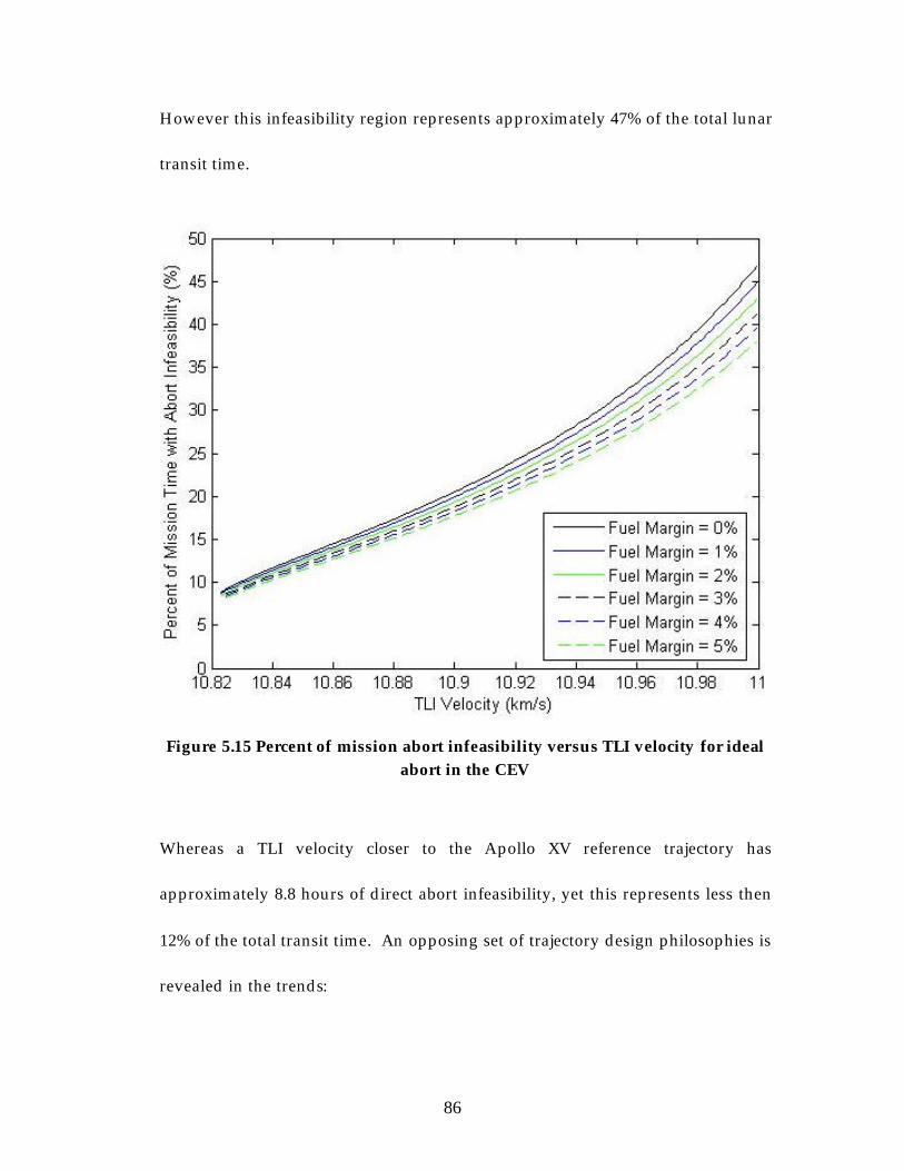
86

However this infeasibility region represents approximately 47% of the total lunar

transit time.

Figure 5.15 Percent of mission abort infeasibility versus TLI velocity for ideal

abort in the CEV

Whereas a TLI velocity closer to the Apollo XV reference trajectory has

approximately 8.8 hours of direct abort infeasibility, yet this represents less then

12% of the total transit time. An opposing set of trajectory design philosophies is

revealed in the trends:

87

1) Design for high final TLI velocity (reducing transit time) with the

theory that shorter transit time equates to statistically reduced possibility for an

emergency abort scenario occurring.

2) Design for low final TLI velocity (lengthening transit time) with

the idea that increasing the abort feasibility over the mission out weighs the

added statistical chances of an emergency abort scenario occurring.

Present results suggest that the first design philosophy would generally

have prohibitively high ∆V requirements. ∆V fuel budgets for that end of the

spectrum range as high as 2 km/s in excess of Apollo mission parameters. A

more beneficial strategy would be to blend the two design philosophies, by

designing for a higher TLI velocity to reduce transit time but build in a larger

fuel margin to in effect decrease transit time while holding the abort feasibility

envelope constant. Further system reliability studies would be required to

determine trade offs between shorter transit time combined with reduced abort

capabilities, versus longer transit times containing much higher abort feasibility

options.

5.4. Expedited Return During Feasible Direct Aborts

The available excess fuel was divided up into two burn portions, one

portion to accelerate the transfer orbit to a higher energy trajectory, and one to

88

decelerate just prior to re-entry to match re-entry corridor conditions. This

division of available fuel is shown in Figure 5.16 for the second segment of abort

feasibility for the Apollo nominal abort scenario. Mission hour time was utilized

as the independent variable for these plots such that if a direct abort is initiated

at ‘X’ hours into the translunar injection, data for that position along the

trajectory can easily be found by referencing mission time on the plots. The

acceleration burn to attain a higher energy return trajectory is the difference

between the solid and dotted line, while the ∆V shown by the dotted line is that

required just prior to re-entry to match corridor conditions. Of note on this plot

is the difference in the relative magnitude of the acceleration and deceleration

burns with respect to the near-Earth mission segment due to the large radial

distances from Earth during this portion of the lunar transit. Angular

momentum must be conserved, thus a small impulse of ∆V far away from Earth

translates to a much larger ∆V required to negate the increased angular

momentum in close proximity to Earth, namely, just prior to re-entry to assure

compliance with re-entry corridor conditions.

89

Figure 5.16 Apollo XV division of ∆V high energy return

A higher energy return trajectory enables a reduction in return to re-entry

time for the spacecraft. Also plotted as a function of mission hour, this reduction

in flight time can be examined in Figure 5.17, where the dotted line represents

the return time to re-entry of a standard abort, and the solid line represents the

return time for the optimized higher energy trajectory.

90

Figure 5.17 Apollo XV nominal abort, higher energy trajectory reduction in return time

The first segment of abort feasibility has been omitted from the

optimization as the altitude range is fairly small, and since the CEV transit time

through this altitude range is on the order of 3-4 minutes, no optimization of

excess fuel was required. An abort during the first segment of abort feasibility

during the mission will require fast recognition of the problem and action, and

has already been deemed highly improbable. If the near-Earth abort window is

missed, approximately 10-15 hours are required until the next region of abort

91

feasibility. Secondly, simply reflecting the orbit via the abort will yield the same

flight time to re-entry of 3-4 minutes; which is short enough not to require

acceleration (recalling that engine burns are considered to be instantaneous for

the model). The instantaneous change of ∆V assumed in the astrodynamic

model is fine for flight times on the order of hours; however with a flight time of

4 minutes or less, engine burn time will become a large factor requiring further

study. Thus if a direct abort can be executed in such a short time a simple

reflected abort is all that is necessary due to extremely short flight times.

Upon examining Figure 5.17 a best case reduction in flight time of

approximately five hours is apparent. However this is for the Apollo spacecraft,

taking into account the additional abort capabilities of the CEV, further benefits

can be realized. Figure 5.18 shows the division of ∆V for an optimized higher

energy return trajectory from an ideal abort method in the CEV.

92

Figure 5.18 CEV division of ∆V high energy return

Figure 5.19 illustrates the benefit in return time of flight for the optimized

higher energy trajectories for the CEV. As before, the dotted line represents the

standard direct abort return time, while the solid line represents the achievable

return time. Lastly to quantify the gain in return time Figure 5.20 shows a plot of

the reduction in flight time via the higher energy transfer orbit.

93

Figure 5.19 CEV ideal abort, higher energy trajectory reduction in return time

Figure 5.20 Reduction in return time for ideal CEV abort as a function of mission time of abort initiation

94

A factor of 12% reduction in return time could potentially be vital

depending on emergency situational concerns, fading life support,

environmental conditions, etc. Most importantly this higher energy return

trajectory is simply using fuel that would otherwise remain in the tanks un-

utilized, wasted. In practicality the direct abort ∆V maneuver and the ∆V

maneuver to initiate the higher energy transfer could be combined into a single

engine burn.

5.5. Return During Infeasible Region, Pseudo-Direct Aborts

The very nature of the problem holds grim outlook for this analysis in

terms of finding a panacea trajectory to return to Earth. The model was created

with a Sequential Quadratic Programming (SQP) method of minimization in an

attempt to search the abort trajectory design space for any unforeseen feasible

options. It has already been established that even for an ideal abort method the

CEV does not have the effective ∆V capability to perform a direct abort in this

region to the translunar trajectory. The optimization sought to discover any

feasible trajectories utilizing two or more segments, in effect, pseudo-direct

aborts.

The objective function for the optimization scheme was that of time of

flight for return. This was chosen because if minimizing ∆V was utilized, many

95

trajectories would have been expected, however all with much too long time of

flight characteristics. A well known tradeoff in astrodynamics is that between

time of flight and ∆V required for the maneuver, the lower the ∆V for the

maneuver, the longer the time of flight to reach the destination. For the case of

finding a return trajectory for the CEV, the shortest time of flight was desirable.

Namely due to the length of the infeasibility region; at approximately eight hours

long any feasible trajectory would need a time of flight for return to be less then

16 hours. This is assuming a worst case scenario where a direct abort is required

just after completion of the TLI burn. If the pseudo-direct abort has a longer time

of flight than simply waiting until the threshold of direct abort feasibility and

returning on a direct abort, than it is not a reasonable choice.

Inherent to the optimization is significant computational time due to

many iterations of the objective function. In the case of this model, the objective

function was required to be solved twice for each design iteration, once for the

actual objective function, and once again as a component of the nonlinear

constraint. In consequence, specific data points were chosen along the trajectory

to analyze.

Nearly 70 data points were evaluated in close proximity to the feasibility

threshold due to the lower required ∆V for a direct abort in these regions.

Although prohibitively high for a direct abort, the required ∆V for a direct abort

was low enough to be considered potentially achievable via pseudo-direct abort

96

methods. Figure 5.21 illustrates some of the data points, represented by vertical

lines, based on mission time of a theoretical emergency requiring an attempted

pseudo-direct abort.

Figure 5.21 CEV ideal abort, example data point locations

Each of 23 specific mission hour times was evaluated at potentially three

different trajectory options, two, three, or four intermediate burns. Not every

trial run resulted in a closed trajectory sequence. As the pseudo-direct abort

method is built one trajectory segment at a time, it was possible and quite likely

97

for the trajectory not to close. Meaning the optimizer could not find either a local

or global minimum. In this case, since the SQP method is gradient based, it is

reasonable to assume it should converge on any possible solution fairly quickly,

and a maximum of 1000 was set on the function evaluations.

Out of 23 data points including three different burn combinations at each

point, 14 trajectories did close. Of those 14, six of the trajectories required far too

much ∆V. The model was set up such that if the ∆V constraint was violated but a

closed trajectory sequence was found it would report the required ∆V. Of other

eight trajectories returned, six violated the ∆V constraint, leaving two viable

trajectories. However of the six violating the ∆V constraint, the maximum was

only 1.5 kilometers per second, higher, or approximately 30%. Table 5.6 gives the

data of the best five trajectories found and their associated performance gains

Table 5.6 Pseudo-direct abort trajectories

A major point of note is the first trajectory is in fact a feasible closed

pseudo-direct abort trajectory. In addition it also affords a 27% savings in return

time. The second trajectory is also worthy of note, specifically due to its ability to

save almost 14% in return time via an approximately 5% fuel increase.

98

These results, while not a very high success rate regarding the number of

data points vs. number of useful trajectories, do hint at a small niche of trajectory

design space. That although a single burn direct abort is not feasible, it is

possible to slightly ‘gray’ the feasibility boundaries utilizing intermediary

trajectories to form a pseudo direct abort sequence.

When viewing the raw trajectory data and interesting point emerges. The

algorithm utilized worked backwards form the re-entry corridor through the

pseudo-direct abort sequence to the original abort initiation position. In this

matter there is a trajectory matching burn that is calculated from the reverse

sequence such to match the entire sequence to the original outbound TLI prior to

abort, in effect closing the trajectory and defining a solution. Examining the ∆V

burn data and the optimizer selected coast times for the intermediate trajectories

reveals that the viable pseudo-direct abort trajectories closely mimic the form of

the direct abort trajectory. They all have a single major abort initiating burn,

followed by a long coast. However, subsequent trajectory segments are for the

most part very short coasting times, on the order of minutes, and tend toward

radii closer to Earth implying that the feasible pseudo-direct aborts in general

form verify that the direct abort method is in fact a correct strategy. By allowing

the optimizer to determine coast times and ∆V maneuvers, it is able to select the

best method for an abort, and when its selected method mimic the original

conceived direct abort, it verifies the concept. However few the actual closed

99

pseudo-direct abort trajectories were, they did serve to verify the direct abort

method. The pseudo-direct abort model was created to allow for any number of

intermediary burns in the trajectory sequence. A range of two to four was

chosen based on reliability and risk of firing main propulsion systems numerous

times in an emergency situation. It was presumed that the least number of ∆V

maneuvers required was preferred. To that effect the design variable vectors

were set up as a function of desired number of burns, flexible to any number.

Thus, verification of both models against each other was possible. By picking a

data point in the feasible region and setting the number of intermediary burns to

one, the model created for the infeasible region requiring a pseudo-direct abort,

should in effect mimic the direct abort model. Upon inputting a feasible data

point at mission hour 8.99, a direct abort trajectory was returned with a time of

flight of 8.58 hours. Which at first glance is within 4.7% of the direct abort model

results; however, referring to Figure 5.20, for a abort initiated at approximately

nine hours mission time, utilizing all available fuel a drop of approximately 0.4

hours is expected in return time. Taking this approximately 0.4 hours into

account with the 8.58, results in approximately 8.98 hours compared to 8.99

hours. Briefly, the pseudo-direct abort study provided a check for any missed

trajectory methods that were not thought of, verified the direct abort concept,

and allowed verification of data for both models.

100

Chapter 6. Conclusions and Implications

Following the comprehensive trajectory analysis presented in Chapter 5;

Chapter 6 details flexibility of the developed model to handle future lunar

missions. In addition, conclusions specific to the CEV are presented along with a

quick overview of possible future work.

6.1. Flexibility of Abort Trajectory Study

With regards to future applications the work completed thus far has been

aimed at creating a resource to be utilized for mission planning and potentially

spacecraft capability for any future lunar missions.

Flexibility between the Apollo spacecraft example and the CEV, as well as

any other lunar bound spacecraft for that matter, can be easily adapted into the

model via mass ratios and ∆V performance data. The spacecraft mass data is

included in the calculat ion of the mission budgeted ∆V for the spacecraft based

on trajectory profile. It is then converted from the budgeted ∆V to an effective

∆V for each type of abort method based on staging mass fractions. The four

abort methods are defined via mass fractions; simply rearranging the mass

fractions can create new abort staging methods.

101

Upon complete evaluation of the four abort methods it is the ideal abort

method which clearly is the primary choice for an abort during a CEV lunar

mission. This method not only provides the maximum effective ∆V, thereby

increasin g feasibility of a direct abort, it also retains the largest possible habitable

volume, and presumably available consumable resources contained on the

LSAM ascent stage, for the duration of the return trajectory.

Another point of note concerning various abort staging methods and their

application to optimized higher energy return trajectories is that of biased ∆V for

the deceleration burn. The vast majority of ∆V expenditure is just prior to re-

entry due to conservation of angular momentum. In close proximity to Earth it

takes a large amount of ∆V to affect a small change in angular momentum. The

consequences of this directly impact the available habitable volume and life

support resources for the crew during a higher energy return trajectory. Since

the accelerating burn requires such little ∆V it is likely that the first module

jettisoned may not be jettisoned until the remainder of its fuel is depleted at the

beginning of the decelerating maneuver. Therefore by virtue of a large bias in

∆V towards matching re-entry corridor conditions, further life support

capabilities than expected from examination of abort staging methods, may exist

for the duration of the return.

In addition to flexibility on spacecraft ∆V determination via mass ratios

and abort methods, the model has been designed with a reasonably wide range

102

of trajectories. Theoretically an infinite number of possible trajectories is

available by varying the translunar injection altitude and velocity. Noting;

however, that velocity should be kept below 11.2 kilometers per second for

manned missions regardless due to reaching near-Earth-space escape velocity

and attaining hyperbolic trajectories. Given the flexibility in spacecraft capability

characterization as well as trajectory definition, this work should be adaptable to

any future manned lunar mission.

6.2. Practicality & Conclusions for the CEV

Originally constructed around Apollo mission data as a basis, the model

has since been updated with all available CEV mass estimations and propulsion

system forecasted capabilities. Rationale for a necessitating a direct abort has

been explained. Emergency situations can arise from mechanical,

environmental, or other concerns such as health. If such a situation does arise,

several staging options have been examined and their effective ∆V capabilities

analyzed. The intent of the study was to characterize the feasibility of a direct

abort situation for the CEV. As such the first objective was an easy inspection

based method by which to ascertain abort feasibility via profile plots like that of

Figure 5.3 which characterize both the ∆V requirements and capabilities of the

spacecraft for various abort staging methods. Next, a SQP optimization scheme

was utilized to best distribute excess fuel margin after a direct abort maneuver in

103

order to attain the fastest return to Earth possible while still within the

constraints of the re-entry corridor. Following optimized higher energy

trajectory return optimization, a trade study was conducted to examine the

effects of varying TLI velocity as well as fuel margin. It was deemed possible to

affect a higher energy TLI trajectory with the same feasibility region as a lower

energy transfer if sufficient fuel margin was budgeted. For a spacecraft such as

the CEV bein g designed for global lunar access, it is likely to be utilized on

missions that are not reaching its propulsion capabilities limits. During such

missions, the ability to decrease transit time may be possible while maintaining

constant abort feasibility profiles via fuel margin.

Another possible concept to consider when designing the CEV is the

sensitivity of fuel margins to specific spacecraft modules on the overall abort

feasibility. To this effect a fuel margin of 5 and 10% was applied to each

propulsion module of the CEV stack; Table 6.1 summarizes the results of this

analysis for the CEV utilizing the ideal abort method.

Table 6.1 Specific module fuel margin sensitivity on abort infeasibility

104

For point of reference the infeasibility duration for the CEV on an ideal abort is

8.32 hours. The service module as well as the LSAM ascent stage both achieve a

relatively marginal gain in abort feasibility via increased fuel margin. However

the mass ratio advantage combined with added propulsive responsibility for the

LSAM descent stage grants a distinct advantage to abort feasibility via increasing

the LSAM descent stage fuel margin. The relative mass of the LSAM DS

compared to the other module, and its added responsibility of performing the

LOI burn to circularize the CEV stack in LLO demands a larger fuel capacity.

Inherently the LSAM DS is the most desirable module to lend a fuel margin;

resulting in a 6.8% and 13.1% increase in abort feasibility from 5 and 10% fuel

margins respectively. The design recommendation of maximizing the fuel

margin for the LSAM DS holds a two fold advantage. Primarily the direct

influence of added fuel margin to increasing abort feasibility; but the

recommendation also inherently improves the possibility of further lunar access

via landing site flexibility.

Converse to the fuel margin advantages is the situation of a spacecraft

mass over budget on design mass. The need to reduce mass of the spacecraft

could be represented by a negative fuel margin. In that respect the same fuel

margin study is expanded into the negative percentage range to represent the

impact on abort feasibility of reducing fuel by a given negative margin. Table 6.2

below parallels Table 6.1; a key focus is the negative reduction in infeasibility

105

region. This negative reduction increases the duration of the abort feasibility

region.

Table 6.2 Specific module negative margin sensitivity on abort infeasibility

Figure 6.1 illustrates the linear behavior of the sensitivity of the abort infeasibility

profiles with respect to fuel margin. The impact of small fuel margins (+ or –

10%) for specific modules on the total available ∆V for an abort can be estimated

from this plot.

Figure 6.1 Impact of fuel margin on available ∆V

106

From another point of view the impact of fuel margin on ∆V available for

abort can be examined based on mass. During the design of the CEV if a

specified amount of mass can be allotted to fuel margin, then Figure 6.2 shows

the percent fuel margin for a specific module that is achieved by adding a

specified amount of mass to the fuel budget. The percent fuel margin attained

from Figure 6.2 can then be examined via Figure 6.1 to yield the final impact on

∆V available for abort from a specified added fuel mass.

Figure 6.2 Percent fuel margin from added fuel mass on a specific module

In the situation of spacecraft module mass being larger than the budgeted design

mass Figure 6.2 can be applied to affect a negative fuel margin as well. For a

107

specified value of kilograms over budget, the percent fuel margin required to

reduce the fuel mass to within overall budgeted mass can be found. Figure 6.1

can than be used to determine the level of increased abort infeasibility from

decreasing the fuel load on a specific module. From the trends in these two plots

two design strategies drop out. The first for the case of positive design margin,

where there exists space in the mass budget to allow addition of fuel. In this case

the optimum choice, from the perspective of maximizing abort feasibility would

be to increase the fuel capacity of the LSAM Descent stage. As is shown in

Figure 6.1, this module yields the greatest benefit to total ∆V available for the

addition of fuel. The second case of a negative design margin where the

spacecraft mass is currently greater then the budgeted design mass, a reduction

in mass must be made. For this case it is clear from Figure 6.2 the ideal module

to reduce the fuel mass of, again from the standpoint of maximizing abort

capabilities, is the LSAM Ascent Stage. This module would allow the lowest

percent fuel margin for a given specified reduction in kilograms of fuel. When

applied to Figure 6.1 as a negative fuel margin, it yields the lowest impact on

total ∆V available. Thus utilizing the studied fuel margin of specific modules can

offer a significant benefit to designing for abort capability during the CEV design

phase.

A further recommendation directly impacting the abort feasibility of the

CEV is that of flexibility of attitude control. Given the technological advances in

108

computing power since the days of Apollo it is not unreasonable to recommend

an inter-module controllability. Given that an emergency situation requiring a

direct abort could include unforeseen circumstances, the ability to control any

given propulsion system from any module would be a distinct advantage for

crew survivability. It would almost negate entirely the need for a manually

targeted direct abort via centering the Earth in the docking reticle. For example

an inter-module propulsion control system could allow the LSAM DS propulsion

system to be controlled by the service module Guidance, Navigation, and

Control (GNC) computer. Or any other combination thereof; the situation of a

manually targeted course correction arose on the Apollo XIII mission due to

limited power constraints prohibiting the use of the GNC computer. The ability

to control the propulsion system of one module from the pilot seat of another

module would not only eliminate this problem and increase abort feasibility, but

also increase reliability via GNC redundancy. In conjunction with recommended

inter-module propulsion controllability would be a recommendation for the

design of robust RCS capabilities. The redundancy of RCS capability between

modules would increase odds of guaranteed abort feasibility. The loss of RCS

ability for any given module should not negate the ability to utilize the primary

propulsion system of the module. If an inter-module GNC capability exists it

follows that the RCS of one module should be designed robust enough such that

control of the entire spacecraft stack can be achieved while a second module is

109

providing primary prolusion. The Apollo spacecraft nearly achieved this

capability; the only exception was the LM AS RCS system was not robust enough

to control the spacecraft while docked with the CSM. Given the mass ratio

changes in the CEV design constituting the decrease in relative size of the SM

compared to the LSAM AS, it would seem reasonable to impose the

recommendation of a more robust RCS system. Overall the design

recommendations of inter-module GNC compatibility as well as completely

robust RCS design for any possible spacecraft module stack combination will

positively impact the ability and available abort options during an emergency

situation.

Lastly, of major accomplishment was the establishment of a pseudo-direct

abort method, opening up the possibility for the fast return of a spacecraft to

Earth via intermediary trajectories. The use of the SQP optimizer allowed

generic trajectory definition, in an effort to look for other trajectory methods not

previously considered. Given the CEV’s improved abort feasibility over that of

the Apollo spacecraft; the possibility exists to potentially perform a pseudo-

direct abort entirely within the Earth’s magnetosphere. This method of abort

would definitely be recommended in the case of abort due to solar radiation

concern and consequently bears value in future mission design studies.

As a side benefit from the need to create this second optimizer as a

completely autonomous model, it enabled the verification of trajectory

110

information from the original model. This combined with comparison of

trajectory profiles to both Apollo flight data and Lambert’s method trajectory

solutions, yields a high confidence in the model.

6.3. Future Work

There are two limitations to the models created in this study. First they

are both based in 2-D, assuming all maneuvers occur in the plane of departure

for the translunar trajectory. Plane changes are accounted for in a “worst case”

plane change factor method, however a fully 3D model could provide further

accuracy for abort feasibility characterization. Secondly, the primary motivation

in this study has been to bring the crew of the spacecraft home as quickly and

safely as possible. In line with this reasoning it was deemed more desirable to

land anywhere on the earth than remain in space during an emergency situation.

To this effect, landing foot print magnitude or location has been neglected.

While its inclusion would require a specific launch date, the inclusion of landing

site tracking in the trajectory analysis could add options for mission control. If

for instance a direct abort was required, but there exists enough time to loiter in

orbit and land in a predetermined location this may be a desirable function to be

included in the model.

111

Further work may cover trajectory analysis through re-entry taking into

account aero-thermodynamic effects. Or perhaps examine off design trajectory

re-entry. Fully understanding the extents of limitations on flight path angle and

re-entry velocity could be useful in abort situations. Allowing a higher re-entry

velocity could enable a faster return by utilizing less fuel to slow the spacecraft at

the re-entry interface.

This study has characterized the feasibility and requirements for various

abort trajectories as well as offered optimization of these trajectories. The

newfound understanding can offer the crew of any future manned lunar mission

the best possible chances for a safe return in the event of an abort scenario.

112

Bibliography

1 “Exploration Systems Architecture Study: Final Report (ESAS).” NASA, November 2005. NASA-TM-2005-214062. www.sti.nasa.gov 2 “Crew Exploration Vehicle,” NASA RFP NNT05AA01J, Attachment J-1, http://prod.nais.nasa.gov/cgi-bin/eps/sol.cgi?acqid=113638 3 Lozier, David. Galal, Ken. “Lunar Prospector Mission Design and Trajectory Support.” AAS 1998-323 4 Hoekstra, T.B. “The Abort Capabilities of the Apollo Spacecraft on the Translunar Trajectory.” Bellcomm, Inc., TM-68-2013-3. June 25 th 1968. 5 Anselmo, D.R. Baker, M.K. “Translunar and Lunar Orbit Abort Trajectories for Apollo 14.” Bellcomm, Inc., B70-12019, December 7th 1970. 6 Stern, R. J. “Preliminary Evaluation of SM/RCS Capability to Abort to Earth Entry from the Relaxed Free Return Profile.” Bellcomm, Inc., B70-09084, September 30th 1970. 7 Bass, R. A. “Optimization of Hybrid Trajectories for the Apollo Mission Under a DPS Abort Constraint.” Bellcomm, Inc., B69-02018, Febraury 7th 1970. 8 Babb, Jr., Gus R. “Translunar Abort Techniques for Non-Free-Return Missions.” NASA, TM X-1806 9 Foggatt, Charles E. “Manual Abort Maneuvers During the Translunar Coast Phase of a Lunar Mission.” NASA MSC Internal Note 66-FM-140, November 21st 1966. 10 Vaughan, W. W., Niehuss, K. O., Alexander, M.B. “Spacecraft Environments Interactions: Solar Activity and Effects on Spacecraft” NASA Reference Publication 1396, November 1996 11 “New Vision for Space Exploration Program Announcement.” President George W. Bush, January 14th 2004. http://www.whitehouse.gov/news/releases/2004/01/20040114-3.html

113

12 Larson, Wiley J., Pranke, Linda K. Human Spaceflight: Mission Analysis and Design. McGraw-Hill, New York. 13 Apollo by the Numbers: A statistical Reference,” NASA Historical Reference, SP-4029, Table: Launch Vehicle/Spacecraft Key Facts. http://history.nasa.gov/SP-4029/Apollo_18-12_Launch_Vehicle-Spacecraft_Key_Facts.htm 14 “Apollo LM” http://www.astronautix.com/craft/apollolm.htm September 19th 2005. 15 “Apollo CSM” http://www.astronautix.com/craft/apollocsm.htm September 19th 2005. 16 Bate, Roger R., Mueller, Donald D., and White, Jerry E. Fundamentals of Astrodynamics, Dover Publications, New York, 1971. 17 Vinti, John P., Orbital and Celestial Mechanics, Volume 177 in Progress in Astronautics and Aeronautics, AIAA, Reston, 1998. 18 Escobal, Pedro R., Methods of Orbit Determination, Volume John Wiley & Sons, New York, 1965. 19 Vallado, David A. Fundamentals of Astrodynamics and Applications, Second Edition. Microcosm Press/Kluwer Academic Publishers, El Segundo, 2001. 20 Beksinski, E. David; Starkey, R. P.; Lewis, M.J. ”Characterization of Feasibility, Methods, and Requirements for Lunar Mission Abort Trajectories” AIAA/AAS Space Flight Mechanics Conference, Tampa, January 22nd 2006. AAS -114 21 Puetrobon, Steven S., “Lunar Orbit Propellant Transfer,” Small World Communications, 1999. 22 “Preliminary Apollo Abort Study Trajectory Analysis.” Space Technology Laboratories, Inc., N79-76209, November 12th 1963. 23 “Apollo by the Numbers: A statistical Reference,” NASA Historical Reference, SP-4029, Table: Translunar Injection. http://history.nasa.gov/SP-4029/Apollo_18-24_Translunar_Injection.htm