Behavioral Micro-SimulationBehavioral Micro-Simulation

1

Jose Holguin-Veras, Ph.D., P.E.William H. Hart Professor

VREF’s Center of Excellence for Sustainable Urban Freight Systems

Center for Infrastructure, Transportation, and the Environment

Rensselaer Polytechnic Institute

jhv@rpi.edu

Main goals

To produce a reasonable guess of freight traffic in metropolitan areas using:Freight trip generation estimates (using NCFRP 25

models)Known delivery patterns, such as tour length

distributions by industry sectors (obtained from data collected by RPI from carriers and receivers)

Observed traffic counts at key corridorsThe BMS was originally developed to assess the

impacts of alternative policies to foster off-hour deliveries (7PM to 6AM)

2

Key components

Freight trip generation (FTG): estimated using the NCFRP 25 models and Zip Code Business Pattern data

Synthetic population of carriers (and receivers, if needed) is createdUsing the data collected by RPI, the sample data is

used to create the population of carriers needed to make all deliveries in the metro area

The origin of the deliveries are set to be the locations were warehouses and distribution centers are located

Delivery tours are created:Match the tour length (number of stops) by industry

sectorMatch the number of deliveries by ZIP code (or any

other level of geography used)

3

Graphically: Freight Trip Generation4

Graphically: Synthetic population of carriersDifferent industry sectors have different tour

lengthsNYC and NJ (Holguin-Veras et al. 2012):

Average: 8.0 stops/tour; 12.6% do 1 stop/tour; 54.9% do < 6 stops/tour; 8.7% do > 20 stops

Synthetic population match observed traffic and FTG

5

Tour simulations

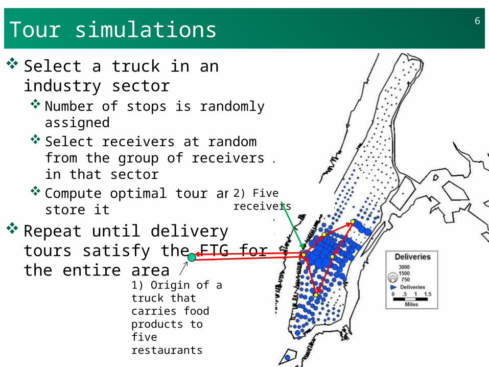
Select a truck in an industry sector Number of stops is randomly

assigned Select receivers at random from

the group of receivers in that sector

Compute optimal tour and store it Repeat until delivery tours

satisfy the FTG for the entire area

6

1) Origin of a truck that carries food products to five restaurants

2) Five receivers

Example: Use of the BMS in the OHD project

BMS use in the off-hour delivery project8

Carrier/receiver synthetic generation Randomly select industry segment

o Generate/locate carriero Generate/locate receivers to serve

 

Receiver behavioral simulation Model receiver’s decision to accept OHD

Carrier behavioral simulation Compute costs for base case and mixed operation Model carrier’s decision

Repeat for another carrier-receivers set

End

Change incentives, reset participation counts

Define range of incentives to receivers for OHD

Ordinal logit model (Holguin-Veras et al 2013)

Regular-hour receiver

Off-hour receiver

 a) Base case (no OHD) b) Mixed operation

 Carrier depotLegend:

Output: Joint Market Share (JMS) of OHD Receivers Market Share (RMS) at TAZ level

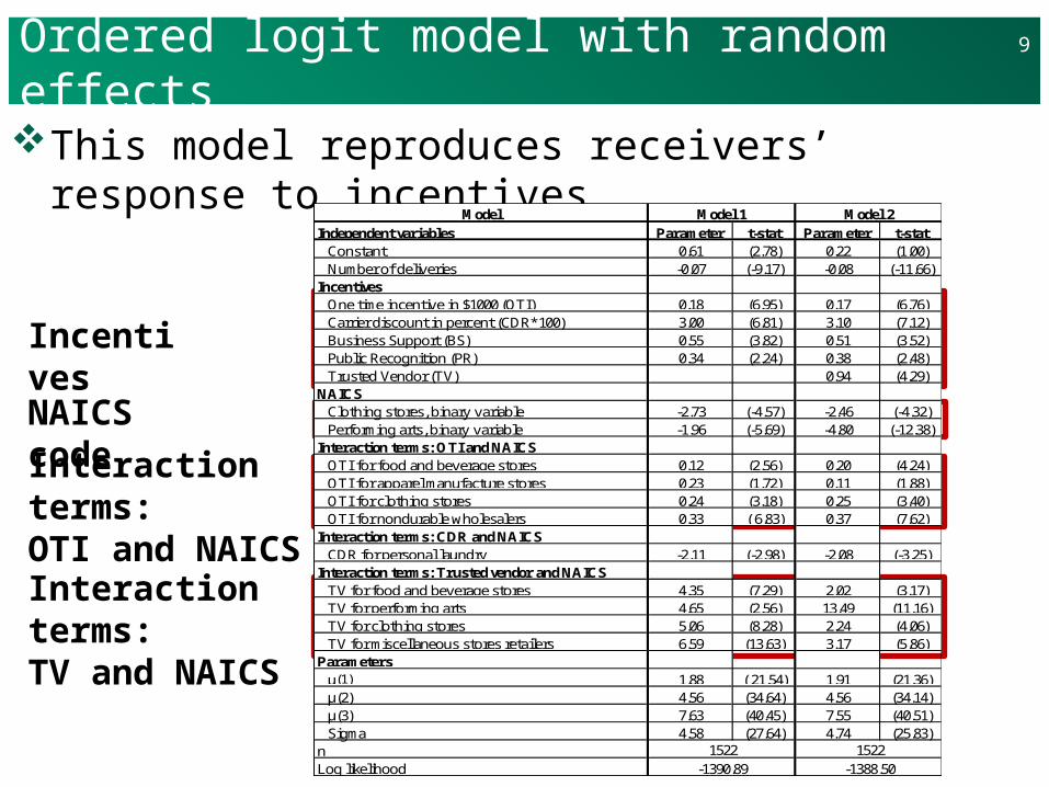
Ordered logit model with random effects

This model reproduces receivers’ response to incentives

9

ModelIndependent variables Parameter t-stat Parameter t-stat

Constant 0.61 (2.78) 0.22 (1.00)Number of deliveries -0.07 (-9.17) -0.08 (-11.66)

IncentivesOne time incentive in $1000 (OTI) 0.18 (6.95) 0.17 (6.76)Carrier discount in percent (CDR*100) 3.00 (6.81) 3.10 (7.12)Business Support (BS) 0.55 (3.82) 0.51 (3.52)Public Recognition (PR) 0.34 (2.24) 0.38 (2.48)Trusted Vendor (TV) 0.94 (4.29)

NAICSClothing stores, binary variable -2.73 (-4.57) -2.46 (-4.32)Performing arts, binary variable -1.96 (-5.69) -4.80 (-12.38)

Interaction terms: OTI and NAICSOTI for food and beverage stores 0.12 (2.56) 0.20 (4.24)OTI for apparel manufacture stores 0.23 (1.72) 0.11 (1.88)OTI for clothing stores 0.24 (3.18) 0.25 (3.40)OTI for nondurable wholesalers 0.33 ( 6.83) 0.37 (7.62)

Interaction terms: CDR and NAICSCDR for personal laundry -2.11 (-2.98) -2.08 (-3.25)

Interaction terms: Trusted vendor and NAICSTV for food and beverage stores 4.35 (7.29) 2.02 (3.17)TV for performing arts 4.65 (2.56) 13.49 (11.16)TV for clothing stores 5.06 (8.28) 2.24 (4.06)TV for miscellaneous stores retailers 6.59 (13.63) 3.17 (5.86)

Parametersµ(1) 1.88 ( 21.54) 1.91 (21.36)µ(2) 4.56 (34.64) 4.56 (34.14)µ(3) 7.63 (40.45) 7.55 (40.51)Sigma 4.58 (27.64) 4.74 (25.83)

nLog likelihood -1390.89 -1388.50

1522

Model 1 Model 2

1522

Incentives

Interaction terms:OTI and NAICS

NAICS code

Interaction terms:TV and NAICS

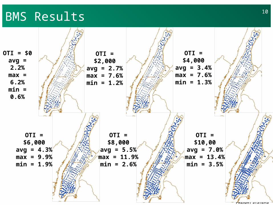
BMS Results10

OTI = $0avg = 2.2%max = 6.2%min = 0.6%

OTI = $2,000avg = 2.7%max = 7.6%min = 1.2%

OTI = $4,000avg = 3.4%max = 7.6%min = 1.3%

OTI = $6,000avg = 4.3%max = 9.9%min = 1.9%

OTI = $8,000avg = 5.5%

max = 11.9%min = 2.6%

OTI = $10,00avg = 7.0%

max = 13.4%min = 3.5%

Example: Geographically Oriented Incentives

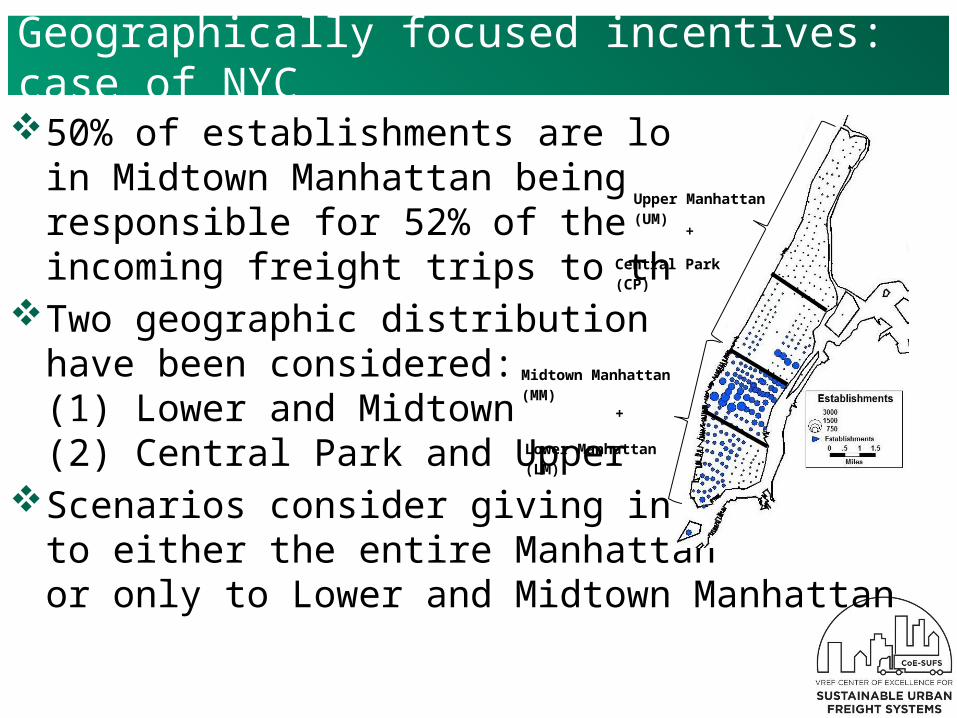
Geographically focused incentives: case of NYC50% of establishments are located

in Midtown Manhattan being responsible for 52% of the incoming freight trips to the city

Two geographic distribution have been considered: (1) Lower and Midtown (2) Central Park and Upper

Scenarios consider giving incentivesto either the entire Manhattanor only to Lower and Midtown Manhattan

Lower Manhattan (LM)

Midtown Manhattan (MM)

Central Park (CP)

Upper Manhattan (UM)

 +

+

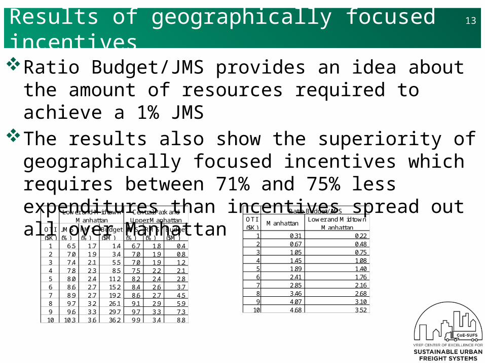
Results of geographically focused incentivesRatio Budget/JMS provides an idea about the

amount of resources required to achieve a 1% JMS

The results also show the superiority of geographically focused incentives which requires between 71% and 75% less expenditures than incentives spread out all over Manhattan

13

OTI ($K)

JMS (%)

RMS (%)

Budget ($M)

JMS (%)

RMS (%)

Budget ($M)

1 6.5 1.7 1.4 6.7 1.8 0.4 2 7.0 1.9 3.4 7.0 1.9 0.8 3 7.4 2.1 5.5 7.0 1.9 1.2 4 7.8 2.3 8.5 7.5 2.2 2.1 5 8.0 2.4 11.2 8.2 2.4 2.8 6 8.6 2.7 15.2 8.4 2.6 3.7 7 8.9 2.7 19.2 8.6 2.7 4.5 8 9.7 3.2 26.1 9.1 2.9 5.9 9 9.6 3.3 29.7 9.7 3.3 7.3 10 10.3 3.6 36.2 9.9 3.4 8.8

Lower and Midtown Manhattan

Central Park and Upper Manhattan OTI

($K)Manhattan

Lower and Midtown Manhattan

1 0.31 0.22 2 0.67 0.48 3 1.05 0.75 4 1.45 1.08 5 1.89 1.40 6 2.41 1.76 7 2.85 2.16 8 3.46 2.68 9 4.07 3.10

10 4.68 3.52

Ratio Budget/JMS

Example: Self-Supported Freight Demand

Management

Self supported freight demand managementA self-supported freight demand management

system (SS-FDM), is one that generates the funds required for a continuing improvement towards sustainability

The incentives to be handed out to the receivers are generated by a toll surcharge to the vehicles that travel in the regular hours

The analyses consider tolls to only trucks (per axle) or both; trucks and cars. Finally, different levels of toll collection efficiency were also considered

15

Results: tolls to trucks (per axle)

Toll collection 100%

Toll collection 75%

16

$1 $2 $5 $8 $10

$0 7.1% 8,467 $0.00 $0.00 $58.08 $116.16 $290.40 $464.63 $580.79

$1,000 7.6% 9,031 $5.65 $1.88 $57.78 $115.56 $288.91 $462.26 $577.82

$2,000 8.2% 9,783 $26.32 $8.77 $57.39 $114.77 $286.93 $459.10 $573.87

$3,000 8.8% 10,463 $59.89 $19.96 $57.03 $114.06 $285.15 $456.23 $570.29

$4,000 9.5% 11,265 $111.95 $37.32 $56.61 $113.21 $283.04 $452.86 $566.07

$5,000 10.3% 12,209 $187.14 $62.38 $56.11 $112.22 $280.55 $448.89 $561.11

$6,000 11.0% 13,058 $275.51 $91.84 $55.66 $111.33 $278.32 $445.31 $556.64

$7,000 11.9% 14,175 $399.58 $133.19 $55.08 $110.15 $275.38 $440.62 $550.77

$8,000 12.8% 15,200 $538.65 $179.55 $54.54 $109.08 $272.69 $436.30 $545.38

$9,000 13.7% 16,279 $703.14 $234.38 $53.97 $107.94 $269.85 $431.76 $539.70

$10,000 14.9% 17,754 $928.70 $309.57 $53.19 $106.39 $265.97 $425.56 $531.95

Freight vehicle surcharge per axle:One-time-incentive

% OHDOHD tours (year)

Total incentive

budget

Yearly incentive

budget

Yearly toll revenues (car surcharge = $0)

$1 $2 $5 $8 $10

$0 7.1% 8,467 $0.00 $0.00 $77.44 $154.88 $387.19 $619.51 $774.39

$1,000 7.6% 9,031 $5.65 $1.88 $77.04 $154.09 $385.21 $616.34 $770.43

$2,000 8.2% 9,783 $26.32 $8.77 $76.52 $153.03 $382.58 $612.13 $765.16

$3,000 8.8% 10,463 $59.89 $19.96 $76.04 $152.08 $380.19 $608.31 $760.39

$4,000 9.5% 11,265 $111.95 $37.32 $75.48 $150.95 $377.38 $603.81 $754.76

$5,000 10.3% 12,209 $187.14 $62.38 $74.81 $149.63 $374.07 $598.51 $748.14

$6,000 11.0% 13,058 $275.51 $91.84 $74.22 $148.44 $371.09 $593.75 $742.19

$7,000 11.9% 14,175 $399.58 $133.19 $73.44 $146.87 $367.18 $587.49 $734.36

$8,000 12.8% 15,200 $538.65 $179.55 $72.72 $145.43 $363.59 $581.74 $727.17

$9,000 13.7% 16,279 $703.14 $234.38 $71.96 $143.92 $359.80 $575.68 $719.60

$10,000 14.9% 17,754 $928.70 $309.57 $70.93 $141.85 $354.63 $567.41 $709.26

Yearly toll revenues (car surcharge = $0)Freight vehicle surcharge per axle:

One-time-incentive

% OHDOHD tours (year)

Total incentive

budget

Yearly incentive

budget

Note: The shaded cells represent non-feasible combinations of financial incentives to receivers and tolls.

Results: tolls to trucks (per axle) and cars

Toll collection 100%

Toll collection 75%

17

$1 $2 $5 $8 $10

$0 7.1% 8,467 $0.00 $0.00 $382.94 $460.38 $692.69 $925.01 $1,079.89

$1,000 7.6% 9,031 $5.65 $1.88 $382.54 $459.59 $690.71 $921.84 $1,075.93

$2,000 8.2% 9,783 $26.32 $8.77 $382.02 $458.53 $688.08 $917.63 $1,070.66

$3,000 8.8% 10,463 $59.89 $19.96 $381.54 $457.58 $685.69 $913.81 $1,065.89

$4,000 9.5% 11,265 $111.95 $37.32 $380.98 $456.45 $682.88 $909.31 $1,060.26

$5,000 10.3% 12,209 $187.14 $62.38 $380.31 $455.13 $679.57 $904.01 $1,053.64

$6,000 11.0% 13,058 $275.51 $91.84 $379.72 $453.94 $676.59 $899.25 $1,047.69

$7,000 11.9% 14,175 $399.58 $133.19 $378.94 $452.37 $672.68 $892.99 $1,039.86

$8,000 12.8% 15,200 $538.65 $179.55 $378.22 $450.93 $669.09 $887.24 $1,032.67

$9,000 13.7% 16,279 $703.14 $234.38 $377.46 $449.42 $665.30 $881.18 $1,025.10

$10,000 14.9% 17,754 $928.70 $309.57 $376.43 $447.35 $660.13 $872.91 $1,014.76

Yearly toll revenues (car surcharge = $1)Freight vehicle surcharge per axle:

One-time-incentive

% OHDOHD tours (year)

Total incentive

budget

Yearly incentive

budget

$1 $2 $5 $8 $10

$0 7.1% 8,467 $0.00 $0.00 $363.58 $421.66 $595.90 $770.13 $886.29

$1,000 7.6% 9,031 $5.65 $1.88 $363.28 $421.06 $594.41 $767.76 $883.32

$2,000 8.2% 9,783 $26.32 $8.77 $362.89 $420.27 $592.43 $764.60 $879.37

$3,000 8.8% 10,463 $59.89 $19.96 $362.53 $419.56 $590.65 $761.73 $875.79

$4,000 9.5% 11,265 $111.95 $37.32 $362.11 $418.71 $588.54 $758.36 $871.57

$5,000 10.3% 12,209 $187.14 $62.38 $361.61 $417.72 $586.05 $754.39 $866.61

$6,000 11.0% 13,058 $275.51 $91.84 $361.16 $416.83 $583.82 $750.81 $862.14

$7,000 11.9% 14,175 $399.58 $133.19 $360.58 $415.65 $580.88 $746.12 $856.27

$8,000 12.8% 15,200 $538.65 $179.55 $360.04 $414.58 $578.19 $741.80 $850.88

$9,000 13.7% 16,279 $703.14 $234.38 $359.47 $413.44 $575.35 $737.26 $845.20

$10,000 14.9% 17,754 $928.70 $309.57 $358.69 $411.89 $571.47 $731.06 $837.45

Freight vehicle surcharge per axle:One-time-incentive

% OHDOHD tours (year)

Total incentive

budget

Yearly incentive

budget

Yearly toll revenues (car surcharge = $1)

Note: in this case all combinations of financial incentives to receivers and tolls are feasible

Potential Uses

Potential Uses

The BMS will replicate freight traffic in any metro area

The BMS could be used to:Produce realistic estimates of freight VMTAnalyze the impacts of alternative logistical

configurations (using a Urban Consolidation Center, transfers of cargo to environmentally friendly modes like freight bicycles)

Analyze the impacts of retiming of deliveries, or receiver-led consolidation programs by receivers

Analyze the impacts of policies that change operational patterns, technologies, or infrastructure used by carriers

Changes in work hours, limited emission zones, etc.

19

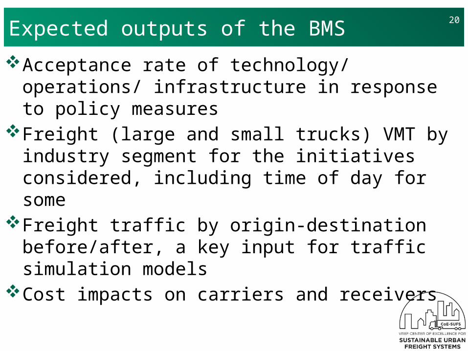
Expected outputs of the BMS

Acceptance rate of technology/ operations/ infrastructure in response to policy measures

Freight (large and small trucks) VMT by industry segment for the initiatives considered, including time of day for some

Freight traffic by origin-destination before/after, a key input for traffic simulation models

Cost impacts on carriers and receivers

20

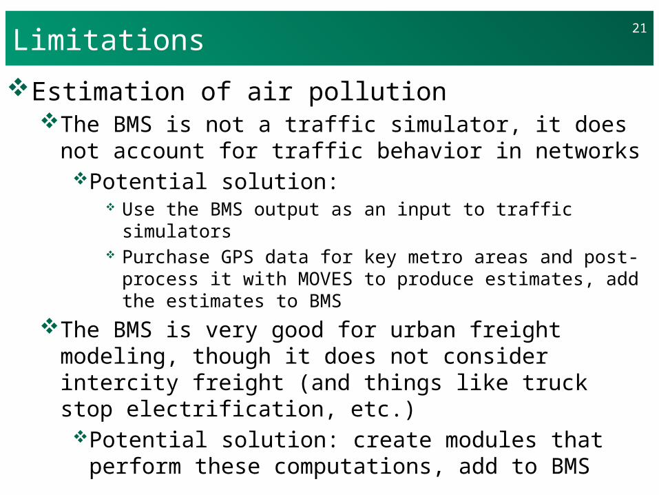
Limitations

Estimation of air pollutionThe BMS is not a traffic simulator, it does not account

for traffic behavior in networksPotential solution:

Use the BMS output as an input to traffic simulators Purchase GPS data for key metro areas and post-process

it with MOVES to produce estimates, add the estimates to BMS

The BMS is very good for urban freight modeling, though it does not consider intercity freight (and things like truck stop electrification, etc.)Potential solution: create modules that perform

these computations, add to BMS

21

Conclusions

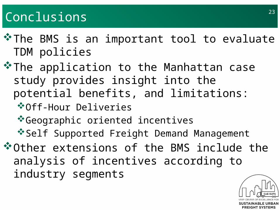
Conclusions

The BMS is an important tool to evaluate TDM policies

The application to the Manhattan case study provides insight into the potential benefits, and limitations: Off-Hour DeliveriesGeographic oriented incentivesSelf Supported Freight Demand Management

Other extensions of the BMS include the analysis of incentives according to industry segments

23

Questions?

24