beef and pork values and price spreads explained

United StatesDepartmentof Agriculture

www.ers.usda.gov

Electronic Outlook Report from the Economic Research Service

LDP-M-118-01

May 2004 Beef and Pork Values and Price Spreads Explained

Abstract

Livestock and meat prices vary more in the short run than costs of production, process-ing, and marketing. ERS research shows that month-to-month changes in livestock andmeat prices are driven by dynamic adjustment. It takes time for prices to adjust, andthey tend to adjust more rapidly when they are increasing than when they are decreasing.When rates depend on direction, price adjustment is called asymmetric. The slow andasymmetric adjustment of prices does not appear to work against livestock producers.This report examines these price transmission issues and also explains price spread cal-culations and analyzes the relationship between marketing costs and livestock prices inthe long run.

Keywords: Beef and pork price spreads, asymmetric price transmission, livestockprices, wholesale meat prices, retail meat prices.

Acknowledgments

This report was improved by comments from Keithly Jones, Suresh Persaud, Janet Perry,and Joy Harwood of the Economic Research Service, from Shayle Shagam of the WorldAgricultural Outlook Board, and from Dawn Thilmany of Colorado State University.The report also benefited from technical review by Dale Simms and production helpfrom Juanita Tibbs.

William Hahn*

* Economist with the Market and Trade Economics Division, Economic Research Service, USDA.

This report examines a number of controversies sur-rounding price spreads for beef and pork. A pricespread is the difference between the cost of an item atone stage of the marketing channel and a differentstage. ERS collects prices at three different stages ofthe marketing chain for beef and pork: the farm, thepacking plant (wholesale), and at the grocery store(retail). These three sets of prices are used to calculatefarm, wholesale, and retail values for beef and pork.These three price levels allow the calculation of threeprice spreads: farm-wholesale, wholesale-retail, andfarm-retail.

High and increasing price spreads often lead to contro-versy. Livestock producers often blame low livestockprices on high price spreads. Consumers blame highretail prices on high price spreads. Increasing pricespreads can both inflate retail prices and deflate farmprices.

Sometimes analysts cite increasing amounts of value-added as a cause of rising price spreads. Consumersshifting demand toward more value-added productswill result in lower percentages of the consumer food

dollar being passed on to farmers. A higher demandfor value-added products and a lower farm share of theconsumer food dollar will not generally lead todecreases in farm prices. Analysts who cite increasingvalue-added as a factor in pork and beef price spreadsmisunderstand how these are calculated.

Price spreads fluctuate greatly from one month to thenext. These short-term fluctuations are consistent withwhat economists call “dynamic price adjustment.” Ittakes time for prices to adjust to changes in economicconditions. With dynamic price adjustment, pricespreads can be temporarily higher or lower than they“ought” to be. Price adjustment dynamics will tend tomove prices so that price spreads go toward wherethey ought to be. One of the important factors thatdetermines how farm and retail prices react to dynamicadjustment is a concept that economists call price dis-covery. In this case, price discovery is about which, ifany, of the stages in the marketing system is mostimportant in determining prices. In simple cases, oneprice reacts first and the others follow. In more com-plex cases, each price can simultaneously influenceand be influenced by the others.

2 • Economic Research Service, USDA Beef and Pork Price Spreads Explained • LDP-M-118-01

Introduction

The basic idea behind price spreads is simple.Consumers, for the most part, do not buy food directlyfrom farmers. The price consumers pay for food isalmost invariably higher than that received by farmers.The farm-to-retail price spread is the differencebetween what the consumer pays and what the farmerreceives. From the consumer’s point of view, the retailprice is the most important. Changes in retail pricesaffect consumers directly. Producers are directlyaffected by the farm price. Why would either careabout price spreads?

Producers expect two things out of a price-spread-reporting system. The first is help with marketingtheir products. The better their knowledge of whatconsumers want from meat, the better producers canmeet consumer expectations. Retail prices or valuesare part of the information producers need to under-stand consumer demand. Price-spread calculationsrequire the collection, calculation, and reporting ofretail prices.

Producers also use price spreads to measure the effi-ciency and equity of the food marketing system.Producers are concerned about getting their fair share.Consumers are also concerned about the efficiency andequity of the food marketing system. All other thingsthe same, consumers would prefer lower prices andproducers higher prices. In mathematical terms, theprice spread is the retail price minus the farm price.We can rearrange the price-spread equation and makeit more useful for farmers or consumers. Consumerscan view their price as the farm price plus spread. Theconsumer equation implies that higher price spreadscause higher retail prices. Farmers can see their priceas the retail price minus spread. The farmer equationimplies that higher price spreads cause lower farmprices. Price spreads can become lower if farm pricesincrease and/or retail prices decrease.

Turning the price-spread definition into a farm-price orretail-price equation is a mathematical exercise. Inorder for this exercise to correspond to something inreality, the price spread has to be something more thanjust the difference between the farm and retail price. Itis. The price spread is the costs and profits of the mar-keting system that moves the farm product from thefarm to the consumer and processes it to its final form.

Innovative technologies can lower costs and, conse-quently, price spreads.

The farm-to-wholesale and wholesale-to-retail spreadsdivide the total costs and profits between packers andgrocery stores. Economic efficiency increases whencosts and profits drop. In theory, changes in pricespreads can help measure changes in the efficiency ofthe beef or pork marketing system. Both consumersand farmers can gain if the food marketing systembecomes more efficient and price spreads drop. Lowerprice spreads can reflect both higher farm prices andlower consumer prices.

One of the problems with implementing a price-spreadcalculation is coming up with a definition for the farmand retail product. At the farm level, hogs and cattlecome in a variety of sizes, ages, grades, and other fac-tors that affect their price. Consumers also have avariety of outlets where they can buy meat, and canoften buy multiple forms of this meat from the sameoutlet. The perfect price-spread system would calcu-late price spreads for all animal types and outlets, andgive information on the relative importance of each ofthe marketing channels. The perfect price-spread sys-tem would require large amounts of data, computingresources, and human time, and consequently wouldbe extremely expensive. The perfect price-spread sys-tem would also require data the government does notcollect. For example, official statistics show only totaldomestic disappearance of meat, which means we donot know how much meat goes through stores and howmuch goes through food service, only the total goingthrough both.

ERS provides two different “compromise” measures ofmeat price spreads. One compromise is to comparethe “average” value of all hogs and cattle sold to the“average” value of pork or beef purchased in all formsfrom all outlets. The Food and Rural EconomicsDivision of ERS calculates price spreads for meats andother foods using this method.1 The major purpose ofthese price spreads is to calculate the farmer’s share ofthe consumer food dollar. The consumer costs of meatare based on research that the Bureau of Labor

Beef and Pork Price Spreads Explained • LDP-M-118-01 Economic Research Service, USDA • 3

How Values and Spreads Are Calculated

1 See www.ers.usda.gov/Briefing/FoodPriceSpreads/

http://www.ers.usda.gov/Briefing/FoodPriceSpreads/

Statistics (BLS) uses to calculate the Consumer PriceIndex (CPI). The consumer market basket is based onperiodic surveys of consumer purchases. Between sur-veys, price spreads are calculated using the assumptionthat the items consumers buy do not change.

ERS’s Market and Trade Economics Division, on theother hand, calculates price spreads based on a stan-dard animal, cut up in a standard way at the packingplant, and sold in standard form through the retailstore.2 These price spreads are the basis of this report.Focusing on a standard animal and marketing channelreduces the amount of data that has to be collectedcompared with that needed to calculate an “average”spread. Spreads based on average costs of beef andpork through all outlets change when the mix of out-lets changes and when the margins in each outletchange. Increasing “average” spreads can be the resultof increasing costs/profits, shifts to more costly chan-nels, or both. Focusing on a single market channelallows one to attribute changing spreads to changes ineconomic performance in that channel. Given that oneis focusing on a single channel, it would be helpful ifthat channel handles a relatively large volume of meat.Grocery stores are an important channel for meatsales, which is one reason that ERS calculates its retailvalue based on grocery-store prices.

Producers also use retail-price information in analyz-ing the end demand for their livestock. Focusing on asingle channel and type of animal makes the retail val-ues more consistent over time and easier to compare.The ERS standard marketing channel is a non-special-ized or generic market. Those producers that are look-ing into market niches could always divert their ani-mals into this “generic” channel. The ERS retail valuerepresents a potential minimum value for more spe-cialized producers.

The quality of animals that producers raise, and thecutting practices at the packing plant and the grocerystore, evolve over time. ERS makes occasionalchanges in its standard animals and standard cuts tobetter reflect current practices. When the standard ani-mals or cuts are changed, ERS recalculates the previ-ous farm, wholesale, and retail values in an effort tomake the historical data consistent with the new prac-tices. The current standard beef animal (farm) price isthe five-market, weighted average for a 35-65%

Choice Steer as reported by USDA’s AgriculturalMarketing Service (AMS). The standard hog (farm)price is the AMS 51-52% base-lean-hog price. Somepeople have complained that these ERS standard ani-mals are now substandard relative to the bulk of themarket. However, the goal of this methodology is tocompare price spreads for a consistent animal overtime, not to compare price spreads for each period’smost “representative” animal.

Wholesale values for beef and pork cuts are also pub-lished by AMS. ERS uses these wholesale values tomake the wholesale composite values. The retail beefand pork cuts that ERS uses in the calculation of itsretail composite prices are relatively low value-addedcuts. All the beef cuts are fresh cuts sold through themeat case. The pork cuts are all fresh except for hamand bacon. Consumers purchase little fresh ham orbellies. (Bacon is cured and smoked pork bellies.) ERSchanges in the standard retail value have been small.The current standard retail product has fewer bonesand less fat than the standard product of the 1970s.The standard retail product has always been a relative-ly low-value-added mix of cuts sold through the retailmeat case.

Before 1980, ERS collected data directly from cooper-ating retail stores. The ERS survey started with 20chains; however, the number declined over time. Thecooperators kept track of the prices of their cuts andthe volume sold of those cuts, and provided ERS withsales-weighted average prices. Stores commonlychange meat prices only weekly. When a store lowersthe price of a cut, it will likely sell more of it. Thesales-weighted price of an item was usually lower thanthe price averaged over weeks.

High costs and loss of cooperators led to a change inERS procedures. Since 1980, ERS has used retailprices reported by the Bureau of Labor Statistics(BLS). BLS data are collected from more outlets thanthe old ERS data and from a statistical sample of out-lets versus self-selected cooperating stores. The self-selected stores ERS used prior to 1980 may have beendifferent from stores in general, and this might haveinduced some degree of unknown bias in the retailprices. However, BLS collects only prices from stores,not sales volume on the individual cuts. It can notchange the weights on its averages to reflect changesin sales volume associated with changes in retailprices.


2 See www.ers.usda.gov/briefing/foodpricespreads/meatprice-spreads/

http://www.ers.usda.gov/Briefing/FoodPriceSpreads/meatpricespreads/

http://www.ers.usda.gov/Briefing/FoodPriceSpreads/meatpricespreads/

This omission led to some concern that using BLSretail prices leads ERS to overstate the retail values forbeef and pork. The Livestock Mandatory ReportingAct of 1999 required that USDA “compile and publishat least monthly (weekly, if practicable) informationon retail prices for representative food products madefrom beef, pork, chicken, turkey, veal, or lamb.” Inresponse, ERS began to buy commercially availableretail-scanner data, which are compiled and publishedon the web. These data have sales-weighted averageprices for beef and pork cuts, which are generally, butnot consistently, lower than BLS prices.

Grocery stores are not required to provide scanner datato ERS, so these data come from a self-selected sam-ple of stores. These stores may have either consistentlyhigher or lower prices than the average supermarket.As with the pre-1980 ERS data, the self-selected sam-ple could induce some unknown bias in the reportedaverage prices.

ERS continues to use the BLS data in calculating pricespreads, also mandated in 1999’s Livestock MandatoryReporting Act. Sticking with the BLS data also makescurrent estimates consistent with those from the 1980sand 1990s.

The retail value used in price spread calculations is theaverage price per pound of all the cuts an animal pro-duces. In other words, the retail value is the averagecost per pound rebuilding the animal with meat partsonly from the grocery store. Animals are not entirelymeat. The further up the marketing chain an animalgoes, the more weight it loses due to the removal ofbone and fat trimming, hides, hair, offal, and the like.For example, a 1,000-pound steer produces 417pounds of retail meat cuts, 110 pounds of edible fat,38 pounds of variety meats, 80 pounds of hide, 40pounds of blood, 175 pounds of inedible fats, and 140pounds of liquids lost during processing (shrinkage).

To make the price comparisons easier, ERS transformsthe farm and wholesale prices to a retail-weight equiv-

alent. The live animal value is the cost of the amountof live animal it takes to produce 1 pound of retailmeat. The ERS conversion factors are 2.4 pounds oflive, Choice steer to produce a pound of “standard”retail beef; and 1.869 pounds of 51-52 % lean hog toproduce a pound of “standard” pork. Some bone andfat trimmings are removed in converting wholesalecuts to retail cuts, so wholesale prices also must beadjusted to a retail-weight basis. The ERS standardconversion is 1.14 pounds of wholesale beef per poundof retail beef, and 1.04 pounds of wholesale pork perpound of retail pork.

Table 1 shows January 2003 price spread figures forbeef and pork and includes two farm values and abyproduct value. Many animal parts that are not meat(hides/skins, tallow/lard, bone meal, and edible/inedi-ble offal) have value. ERS does not track the value ofthese byproducts past the packer level. Most of theseproducts are used as intermediate inputs in the produc-tion of other goods, and tracking their contribution tothe final products demanded by consumers is not feasi-ble. Still, the byproducts have value, and this value isused to calculate the byproduct allowance and net farmvalues in table 1.

The total sales that an animal generates for a packerare the value of its meat and byproducts. ERS calcu-lates the percentage of the animal’s value generated bybyproducts. Call that percentage “x.” The byproductallowance is “x” times the gross farm value. The netfarm value is the gross farm value minus the byproductallowance. You could also calculate the net farm valueby multiplying the gross farm value by the percentageof the animal’s value that is meat, 1-x. For example,in January 2003, the byproducts represented 10 per-cent of a steer’s total wholesale value. The byproductvalue for beef in January 2003 is 9 percent of the grossfarm value while the net farm value is 91 percent ofthe gross farm value. The wholesale-to-retail spread isthe difference between the wholesale value and theretail value. The farm-to-wholesale spread is the dif-ference between the wholesale value and the net farm


Table 1—Recent values and spreads for beef and pork

Values Spreads

Species Month Retail Wholesale Gross farm Byproduct Net farm Total Wholesale- Farm-retail wholesale

Beef Jan-03 339.7 200.4 187.1 18.8 168.3 171.4 139.3 32.1Pork Jan-03 258.2 101.9 64.3 3.5 60.8 197.4 156.3 41.1

value. The total spread is the sum of the farm-whole-sale and wholesale-retail spreads, which can also becalculated by subtracting the net farm value from theretail value.

Price Spreads Versus Gross Margins

ERS has historically stressed that it is calculating pricespreads and not gross margins. Gross margins andprice spreads are related, and increases in gross mar-gins are likely to cause increases in price spreads. Agross margin is the difference between the purchaseand selling price of a product. The farm-to-retail pricespread is the difference between the value of an animalat the farm and its value at the grocery store. Theprice spread looks suspiciously like a gross margin.What makes them different?

Let us start by examining the farm-to-wholesalespread. The farm value is based on a specific type andquality of animal. The ERS standard steer or hog isnot the only type of animal that packers slaughter.Each type of animal has its own value at the farm andproduces a different mix of wholesale products. Everyanimal that a packer buys could have a different farm-to-wholesale spread. In the best-case scenario, theERS farm-to-wholesale price spread represents theaverage gross margin for its standard animal.

The ERS farm-to-wholesale price spread is unlikely tomatch average packer margins on livestock exactly.Different animals will have different gross margins.However, we expect that all the possible gross marginsmove together, so that increases and decreases in thefarm-to-wholesale price spread closely follow packers’overall gross margins. The price spread may be higheror lower than packers’ total gross margins; still, ERSprice spreads and packer gross margins are likely to behighly correlated.

The relationship between grocery stores’ gross marginsand the wholesale-to-retail price spread is likely to beweaker than that between packers’ gross margins andthe farm-to-wholesale price spread. The wholesalevalue is the value for which a packer can sell the stan-dard animal’s meat. A packer that buys a standard ani-mal is going to want to sell all its meat and byproducts.The retail value is the value of that animal’s meat in thegrocery store. However, grocery stores do not buywhole animals. They buy selected cuts of the animal.There is no government data on the mix of cuts thatstores sell. The consensus is that grocery stores tend tosell mostly medium-priced cuts of beef and pork, while

foodservice firms tend to sell either low-priced cuts(fast food) or premium cuts. We expect that ERSwholesale-retail price spreads would likely move in thesame direction as grocery store gross margins.

Some people have raised questions about the shifttoward “case-ready” meats and what that implies forprice-spread calculations. Stores have traditionallypurchased wholesale cuts that need further processingbefore sale to consumers. Case-ready cuts arrive inthe store ready to put directly in the meat case. TheERS wholesale pork composite is based on primalpork cuts and the wholesale beef cuts are subprimalcuts. These primal and subprimal cuts are large piecesof meat that grocery-store butchers trim, cut, and pack-age for retail sale. Packers and other intermediaries arenow trimming, cutting, and packaging large volumesof these retail cuts for sale to stores. A store that usescase-ready meat no longer has to process meat itself.Its employees simply take delivery and stock packagesin the meat case. Those stores that buy case-readymeats are essentially subcontracting out their meatprocessing.

One may also consider the ERS wholesale-retail pricespread as the packer-cuts to retail-cuts price spread.Rather than measuring the efficiency of grocery storesin turning wholesale meat into retail meat, it measuresthe efficiency of grocery stores and their subcontrac-tors in turning wholesale meat into retail meat. Ifcase-ready meat has significant cost advantages, it canlead to improved efficiency of the meat marketing sys-tem and lower wholesale-retail spreads.

Case-ready meat could grow to such an extent that itdominates the market, largely eliminating sales of pri-mal and subprimal cuts. If this happens, ERS willhave to switch its price spread methodology to awholesale-case-ready-to-retail price spread.Something like this happened to the ERS methodologyin the late 1970s. Stores used to buy beef by the halfor quarter carcass. Meatpacking companies developedboxed beef in which the carcasses were broken downto (largely boneless) subprimal cuts. As boxed beefgrew to dominate the market, the ERS standard whole-sale beef switched from a carcass to a mix of boxed-beef cuts.

ERS’s retail values are often used by industry analyststo measure the value of beef and pork to consumers.For example, analysts sometimes multiply the totalamount of pork consumed by the pork value, and callthat figure “expenditures on pork.” The ERS retail


value (and the BLS cut-prices underlying it) are basedon retail market prices. Not all meat is bought throughgrocery stores; meat bought in food service is general-ly more expensive than the same cut bought at retail.In addition, the ERS retail value does not include thevalue-added meat products that stores sell. The ERSretail value does not include cooked and processedmeats sold through the service deli or the meat includ-ed in processed foods. Multiplying ERS retail valuesby consumption will understate total consumer expen-ditures on meat.

While the ERS retail composite is a poor measure ofthe price that consumers pay for beef in general, is it agood measure of what consumers pay for beef in thegrocery store meat case? Probably not. As notedabove, the ERS composites are based on the value ofthe whole animal at the store. If stores buy relativelymore of the expensive parts of the animal, the ERScomposite will understate what consumers pay at gro-cery stores. If stores buy more of the relatively cheap

parts of the animal, then the ERS composite will over-state what consumers pay. It is generally believed thatgrocery stores sell relatively more of the lower-pricedcuts. Further, in the case of beef, the standard ani-mal—the Choice, Yield Grade 2-3 steer—is a higherquality animal. Select or ungraded beef cuts generallysell for less than Choice.

One reason that analysts use ERS retail values as ameasure of “price” is to help separate the value of themeat from the other ingredients and services embed-ded in value-added products and food service. Mostvalue-added and foodservice items are a mix of meatand other foods. For example, eating a hamburgerincreases one’s beef consumption, as well as bread andcondiment consumption. One way of valuing thehamburger’s ingredients to a consumer is to use theretail cost of the ingredients. The service value is thedifference between the ingredient costs and total priceof the hamburger.


The demand for livestock is derived from the demandfor meat. Knowing retail prices and price spreadsfrom farm to retail gives us a clearer picture of whatfactors drive the demand for livestock. Economistsuse price spreads as a measure of gross margins, or atthe very least, an indicator of trends in gross margins.The following discussion assumes that price spreadsand gross margins are the same thing. As noted above,gross margins and price spreads are not in fact thesame thing, but they are likely to be related. Grossmargins represent the profits and costs of the foodmarketing system. Increasing economic efficiencyleads to lower gross margins, by either lowering costsor reducing profits. Since high gross margins implyhigh price spreads, for the purpose of theory, it makeslittle difference whether spreads are gross margins orindicators of gross margins. The following discussionis nontechnical. Technical proofs are in the Appendix.

The discussion of how margins affect livestock andmeat prices is based on the economic concept ofderived demand. In economics, “demand” usuallyrefers to the relationship between what consumerswant to buy, their incomes, and the prices they have topay. Livestock and wholesale meat are used to makeconsumer products. The demand for livestock andmeat is derived from the consumer demand for meatand meat products.

No discussion of economic theory is complete withoutassumptions. One assumption is that the technologyof transforming livestock into meat has a very simpleform, the form inherent in ERS price spread proce-dures. ERS price spread procedures are based on theassumption that there is a fixed yield of meat fromeach kind of animal. We also assume that the longrunprice spread is independent of the volume of livestockprocessed. If we keep the assumption of fixed propor-tions, then derived demand and price spreads are inti-mately related. Under these assumptions, the price oflivestock is the price of meat minus the price spread.Higher price spreads translate into lower prices forlivestock.

How much does an increase in gross margins decreaselivestock prices? It is hard to say. Two factors makemeasuring this effect difficult. The first is producers’supply response. Higher margins would tend to

decrease livestock prices. Lower livestock prices dis-courage livestock production. Lower livestock andmeat production leads to higher prices to consumers.The longrun effect of higher marketing margins is lessproduction (than there would be with lower margins)and some combination of lower farm prices and higherretail prices.

The second complicating factor is that ERS pricespreads are farm-to-supermarket price spreads. Thesupermarket is just one of the outlets for beef andpork. If supermarkets were the only outlets for beef orpork, then a 1-cent rise in margins would translate to a1-cent decline in the derived demand for livestock.From that point, the supply adjustments begin to affectthe market. However, because there are other outletsfor beef and pork, particularly food service and export,a 1-cent increase in spread will translate to a less-than-1-cent decrease in the retail-weight derived demandfor livestock. Higher price spreads from wholesale tothe supermarket will raise supermarket prices. Highersupermarket prices mean less demand for meat fromsupermarkets and make other outlets more competitivefor the consumer’s food dollar. A 1-cent increase inthe wholesale-to-retail spread will decrease deriveddemand for livestock by less than 1 cent.

One of the problems caused by focusing only on farm-to-retail spreads for meat is that it ignores the othersources of derived demand. In theory, we should keeptrack of all the sources of derived demand. Officialgovernment statistics allow us to estimate exports.U.S. Government measures of domestic meat demandtrack the meat that leaves meatpackers and warehousesfor domestic consumers but do not account for thetype of outlet that buys it.

The effect of an increase in the farm-to-retail spreadon the farm price is larger when grocery stores have alarger share of total meat markets. Over time, exportand foodservice markets have become more importantoutlets for U.S. beef and pork. Wholesale-to-retailprice spreads probably have less effect on longrunlivestock prices than they did in the past. On the otherhand, packing plants are by far the largest users ofslaughter animals, the other major use of slaughter ani-mals being the export market. A 1-cent increase in thefarm-to-wholesale spread is likely to translate into a 1-


Price Spreads or Gross Margins in Theory

cent decline (or something very close to that) in thederived demand for livestock.

The theoretical effects of the wholesale-retail marginon the derived demand for livestock are also based onthe assumption that only the wholesale-retail marginchanges—and the margins in the other parts of themarketing channel do not. One can discuss this casein theory; in real life, it is, however, extremely unlike-ly that only the grocery store margin would changeand the others not. For instance, grocery stores andrestaurants may be buying some of the same nonmeatinputs. Increases in the costs of common inputs willincrease costs in all the marketing channels, so thathigher grocery store margins would be associated withhigher margins in the rest of the marketing channel.Inflation generally raises the cost of all items, so thatinflation-driven increases in wholesale-retail grossmargins might be associated with inflation-drivenincreases in other outlets’ margins. If a 1-cent increasein the grocery channel’s margin implies a 1-centincrease in all the other marketing channels’ margins,then derived demand will decline by 1 cent. If a 1-centincrease in the grocery store margin implies differentincreases in the other channels, then derived demandcould drop by more or less than 1 cent.

What effect has the growth of the foodservice andexport markets had on the derived demand for live-stock? As these outlets become more important, their

gross margins have a larger effect on the livestockprice. Consumers shifting their meat consumptionfrom retail stores, a lower-margin source, to food serv-ice, a higher-margin source, may or may not depresslivestock prices. Cattle or hog prices will be depressedif consumers buy less beef and pork when they replaceat-home food preparation with away-from-home foods.If they increase meat consumption as they shift towardfood service, derived demand for livestock—and live-stock prices—will increase.

Price spreads are highly volatile, varying greatlymonth to month. This volatility is difficult to recon-cile with the derived demand and livestock supplyexplanation for price interactions. Therefore, econo-mists explain this volatility with price adjustmentdynamics, wherein it takes time for prices to adjust tochanges in the market. If prices at different parts ofthe market adjust at different rates, then price spreadswill be volatile.

In a market with dynamic adjustment, price spreadscan be temporarily either too high or too low. Supposethat current price spreads are too high. Adjustmentdynamics will tend to move prices to narrow the pricespreads. Price spreads narrow if farm prices rise orretail prices fall. High price spreads now may actuallybe a leading indicator that farm prices are likely toincrease in the near term.


Figures 1 and 2 show monthly gross farm, wholesale,and retail values for beef and pork. All the values forall the meats fluctuate from month to month, but thegeneral trend in nominal prices has been upward.While ERS price spreads are meant to capture thevalue of a “standard” animal over time, inflationmakes comparing 1970s values with more current onesdifficult. The animals remain more or less the same,but the value of money changes. Figures 3 and 4 showthe same set of values corrected for inflation using theConsumer Price Index, or CPI. The general trend aftercorrecting for inflation is downward. The prices thatconsumers pay for beef and pork have increased lessrapidly than inflation. In other words, the real cost ofbeef and pork is declining. Economists assume thatthis downward trend in real prices over the long runshows that the beef and pork production/marketingsystems are becoming more efficient.

What do price spreads show about changes in the effi-ciency of the packer and retail segments of the meatmarketing system? Figures 5-8 show the price spreadsfor beef and pork before and after correcting for infla-tion. The general trends in the noncorrected pricespreads are the same for beef and pork. The totalspreads and the wholesale-retail spreads are increasing

over time. The farm-to-wholesale spreads fluctuate,with a slight upward trend. Because noncorrectedfarm-to-wholesale spreads have shown small growth,the inflation-corrected farm-to-wholesale spreadstrended downward until the mid-1990s. After thattime, both farm-to-wholesale price spreads have trend-ed upward. The wholesale-to-retail spreads for bothbeef and pork have trended upward, even after correct-ing for inflation. The declines in the inflation-corrected farm-to-wholesale spreads largely offset theincrease in the wholesale-to-retail spreads. Therefore,the total price spreads show a weak upward trendwhen corrected for inflation.

The discussion to this point has focused on the meatmarketing system. Much of the decline (relative toinflation) in livestock and meat prices has been drivenby technology changes in agricultural production.Research shows that U.S. livestock farms have becomeincreasingly productive over time (Ahearn et al.; Galeand Kilkenny; USDA-NASS). This increasing produc-tivity explains part of the longrun decline in inflation-adjusted livestock prices. Producers are willing and


Beef values

Figure 1

Cents per pound, retail weights

1970 74 78 82 86 90 94 98 020

50

100

150

200

250

300

350

400

450

Gross farm Retail Wholesale

Pork values

Figure 2

Cents per pound, retail weights

1970 74 78 82 86 90 94 98 20020

50

100

150

200

250

300


What Do 30-Plus Years of Beef and Pork Values and Spreads Say About the Market?


Source: ERS. Source: ERS.


Beef values deflated by the CPI

Figure 3

Cents per pound, retail weight

1970 74 78 82 86 90 94 98 20020

50

100

150

200

250

300

350


Pork values deflated by the CPI

Figure 4

Cents per pound, retail weight

1970 74 78 82 86 90 94 98 20020

50

100

150

200

250

300

350


Beef price spreads

Figure 5

Cents per retail pound

1970 74 78 82 86 90 94 98 20020

50

100

150

200

250

Total Wholesale-retailwholesale Farm-

Pork price spreads

Figure 6

Cents per retail pound

1970 74 78 82 86 90 94 98 20020

50

100

150

200

250




able to supply more animals at lower prices.Economic studies of the meatpacking industry alsodemonstrate increasing productivity, which is consis-tent with the longrun decline in farm-to-wholesalespreads. Lower livestock prices and lower packingcosts have led to lower wholesale prices. While thereare no studies published on meat department produc-tivity, there is evidence of declining productivity ingrocery stores’ overall operations (Fortune Magazine;,Harris et al.; Food Marketing Institute; U.S.Department of Labor, Bureau of Labor Statistics). Adecline in productivity would lead to an increase ingross margins. As productivity declines, grocerystores would use more labor and materials to processwholesale beef and pork into retail beef and pork. Theincreasing costs of processing meat will generally leadto increasing gross margins between the wholesale andretail value of meats.

Some of the measured decline in grocery store produc-tivity is likely a shift in product composition. Grocerystore productivity is measured by comparing laborhours and sales. Grocery stores have switched theirproduct mix over time toward more food service. Partof the apparent decline in total store productivity islikely due to the increasing levels of food service. The

new product mix requires more labor, which wouldlead to lower productivity measures for the store as awhole—regardless of the actual productivity of indi-vidual departments. Wholesale-retail spreads for beefand pork have increased more rapidly than inflation.This kind of increase is consistent with declining pro-ductivity of grocery store meat departments.

Grocery stores seem to be selling more boneless,closely trimmed, and value-added meat cuts and peo-ple have often cited this as a cause of increasingwholesale-retail price spreads. However, this explana-tion is not consistent with BLS procedures and ERScalculations. ERS’s retail beef and pork compositeshave been adjusted to reflect the shift to more closelytrimmed and boneless products. Past retail valueswere adjusted to make them consistent with currentcutting practices. The BLS collects consistent prod-ucts over time. ERS takes the value of these cuts andcalculates retail composites. Although value-addedcuts may be increasingly important to stores and con-sumers, ERS composites are based on a fixed mix of(relatively) low-value-added cuts. One goal of theERS retail price calculation procedure is to give pro-ducers an estimate of the end-use value of their live-stock that is consistent over time. The estimated


Beef price spreads deflated by the CPI

Figure 7

1970 74 78 82 86 90 94 98 020

20

40

60

80

100

120

140


Pork price spreads deflated by the CPI

Figure 8

1970 74 78 82 86 90 94 98 020

20

40

60

80

100

120

140



wholesale-retail spreads for beef and pork have beenincreasing over time. If these spreads included theshift to more value-added products, their increasewould be even greater.

A large part of the decline in real livestock prices hasbeen driven by increasing efficiency on the supplyside. On the derived-demand side, the decline in thereal farm-to-wholesale price spread has increased thederived demand for hogs and cattle, resulting in higher

livestock prices. The increase in livestock demandcaused by more efficient meatpacking has been offsetby the increase in the real wholesale-to-retail spread.But again, the retail meat case is only part of the totaldemand for meat. Total, inflation-corrected pricespreads have increased since the 1970s. If grocerystores were the only outlet for meat, then the increasesin wholesale-retail spreads would have more than off-set the increased efficiency of the packing sector.


Prices and price spreads fluctuate a great deal frommonth to month. In the derived-demand view of priceand price spread interaction, these fluctuations in pricespreads might imply wide swings in the cost of meatprocessing. These frequent, extreme changes in meatprocessing costs are not plausible. Economists fre-quently use “dynamic adjustment” to explain price andprice spread behavior.

The following results are based on statistical models ofdynamic price adjustment. Economists often use sup-ply and demand interactions to analyze how prices andquantities are set. The statistical models used herefocus only on price setting behavior in pork and beefmarkets. The models measure how quantities affectprices in the short run, without measuring how pricesaffect quantities. Beef and pork prices are analyzedseparately. The statistical analysis is based on a “par-tial-adjustment model.” The idea of partial adjustmentactually encompasses the range from “no adjustment”to “complete adjustment.” In practice, the no-adjustment model assumes that this month’s prices(and price spreads) are basically last month’s. Underpartial adjustment, prices this month are somewherebetween the no-adjustment prices and the full-adjust-ment prices.

Sometimes, partial-adjustment models work out to be“overreacting” models. Rather than ending up some-where between the no-adjustment and full-adjustmentvalues, prices may overshoot their full-adjustment val-ues. Another way of looking at these types of modelsis to consider last month’s price as where the price“was,” and this month’s full-adjustment value as wherethe price “ought to be.” Adjustment dynamics look athow prices react to the difference between where theywere and where they “ought to be.”

The models are similar to those estimated previouslyby ERS researchers (Hahn, 1989, 1990; Mathews et al,1999) with some new features. Details on the statisti-cal models are in the Appendix. These models haveasymmetric price dynamics built into them. Theasymmetric part of the model allows prices to adjust atdifferent rates depending on whether they are increas-ing or decreasing. (A price’s adjustment rate can alsodepend on the directions of the other prices.)

The no-adjustment case is defined as this month’sprices being last month’s prices. We have yet to definethe complete- (or full-) adjustment case. One of thereasons that prices fluctuate so much from month tomonth is that livestock and meat supplies fluctuatemonth to month. The complete-adjustment case is thatset of prices and spreads that fully reflects changes inlivestock supplies and other factors. This definition of“complete-adjustment values” is vague. However,when estimating a partial-adjustment model, one hasto measure (directly or indirectly) the complete-adjust-ment values for each period in the data. The completeadjustment values depend on pork and beef produc-tion, the month of the year, and trends. As all thesevariables change from month to month, complete-adjustment values also change. (See the Appendix fortechnical details.)

It is common for increases in livestock supply to befollowed by decreases in supply. With partial adjust-ment to supply and demand shocks, prices can bemore stable than they would be under complete adjust-ment. If prices at different levels adjust at differentrates, partial adjustment can make price spreads morevolatile even while making prices less volatile.

ERS calculates gross-farm, byproduct, wholesale, andretail values. From these, ERS calculates another fournumbers: the net farm value and three price spreads(farm-wholesale, wholesale-retail, and farm-retail).The asymmetric adjustment models are estimatedusing the first four sets of variables. We need four setsof complete-adjustment values to complete the model.Algebra enables any four of the eight price spread sta-tistics to determine the rest. The statistical modelsestimate the complete-adjustment values of the whole-sale value, byproduct value, farm-to-wholesale spread,and wholesale-to-retail spread.

The full-adjustment wholesale and byproduct valueswere made functions of, among other things, pork andbeef production. Month-to-month changes in produc-tion can make the full-adjustment values volatile. Thefull-adjustment price spreads were made smooth func-tions of time. (The month-to-month changes in thefull-adjustment price spreads are small.) Dynamicadjustment is partly self-generating. Differential ratesof adjustment can mean that this month’s price spreads


Price Spreads and Price Dynamics

are quite different from their full-adjustment values.The actual price spread can be either above or belowits full-adjustment value. This month’s actual pricespread is next month’s no-adjustment price spread.Part of next month’s dynamic adjustment will be anattempt to narrow the gap between this month’s pricespread and next month’s full-adjustment value.Narrowing price spreads might require increases in thefarm price. A higher-than-full-adjustment price spreadthis month might be a leading indicator that farmprices could increase next month.

Derived-demand analysis demonstrates that loweringspreads causes some combination of higher farmprices and lower retail prices. In the short run, theopposite can happen: low price spreads can lead tohigher retail prices and/or lower farm prices. In thiscase, the price spread is low relative to its full-adjust-ment value. “Low” actual price spreads can lead towidening of price spreads in later periods. Makingprice spreads wider means lowering farm prices, rais-ing retail prices, or some combination of both. Thedifference between the long- and shortrun results iscaused by dynamic price adjustment.

Two sets of analyses were performed, one using thebeef data and one using the pork data. In each of thesesets of analysis, statistical tests were performed. Thefirst tests attempt to answer the questions: (1) “Doprices exhibit dynamic adjustment?” and (2) “If priceadjustment is dynamic, is it asymmetric?” Prices willbe dynamic if the model has partial adjustment. Priceadjustment is asymmetric if the rates of adjustmentdepend on the direction in which prices are going. Theasymmetric part of adjustment is only possible if thereis partial adjustment in the first place. The completeand no-adjustment cases are both defined as symmetric.

Dynamic adjustment was tested by comparing thedynamic, asymmetric estimates to the complete adjust-ment estimates. The dynamic, asymmetric estimatesare statistically different from the complete-adjustmentones. The asymmetry of the estimates is also statisti-cally significant.

Statistical comparisons of partial adjustment andasymmetry depend on two factors. The first is how farthe estimates are from showing either complete adjust-ment or asymmetry and the second is how accuratelythis difference is measured. This concept is easierexplained using an example. Technically speaking,99.99-percent adjustment is partial adjustment. (Fulladjustment is 100-percent adjustment.) The 0.01-per-

cent difference has little practical effect on priceadjustment. However, this difference will be statisti-cally significant if it is measured accurately enough.An adjustment rate of 10 percent would make a large,practical difference, but if imprecisely measured,might not be statistically significant.

So dynamics and asymmetry are statistically signifi-cant, but do they have large effects on price adjust-ment? To evaluate the “practical” effects of dynamicsand asymmetry, the estimated beef and pork modelswere simulated under the unrealistic scenario wherethe complete-adjustment prices and spreads were fixedfor a long period. If the full-adjustment values arefixed for a long enough time, the actual prices willbecome the full adjustment prices. The length of timeit takes prices to adjust to their full-adjustment valuesand the difference between adjustment times forincreasing and decreasing prices show the practicaleffects of the estimated dynamics and asymmetry.

The model was simulated with full-adjustment valuesfixed for 100 months. All prices converged before theend of the 100 months. None of the prices showsimmediate adjustment. However, pork prices adjustconsiderably faster than beef prices. In all cases forboth species, price-increasing adjustment is quickerthan price-decreasing adjustment. It takes 2 monthsfor pork’s gross farm value to fully adjust when it isincreasing and 5 months when it is decreasing. Pork’swholesale value fully adjusts in 6 months whenincreasing and 10 months when decreasing, whileretail adjustment takes 7 months for increases versus12 months for decreases. Beef price adjustment takesover a year in all cases. Increases in beef’s gross farmvalue take 18 months, while decreases take 29 months.Increases in the wholesale value take 17 months, whiledecreases take 29 months. Retail price increases take21 months; decreases, 32 months.

Dynamic adjustment in prices leads to dynamic adjust-ment in price spreads. Price spreads can be differentfrom their full-adjustment values. If price spreads arebelow the full-adjustment level (that is, too small),price-spread adjustment may lead to lower farm prices.Widening the farm-wholesale spread requires the farmprice to drop or the wholesale price to rise. In thelong run, wide price spreads tend to depress livestockprices. In the short run, large price spreads can be aleading indicator that livestock prices are going to rise.

It is, however, possible that livestock prices are notaffected by price-spread adjustment. For example,


economists commonly use markup models, whereinthe farm price changes first. The wholesale pricedynamically adjusts to the farm price and the farm-to-wholesale price spread. The retail price dynamicallyadjusts to the wholesale price and the wholesale-to-retail price spread. In a markup model, the farm pricedoes not react to dynamic-price-spread adjustment.The simulations above show that farm prices adjustmore quickly than wholesale and retail prices. Thistype of adjustment is what you would expect to see inthe markup case.

One can also build models where the wholesale orretail prices move first and the others follow. Markupmodels and those where retail or wholesale prices leadthe others can be called “leader-follower” models.Leader-follower models imply that one level of themarket is the most important center for price discov-ery. Leader-follower models are special cases of moregeneral models where each price can have a role inprice discovery. Each of the leader-follower modelswas tested against the most general case. None of theleader-follower models passed the statistical tests.Leader-follower models have a relatively simple expla-nation for price discovery. The fact that all these rela-tively simple models failed the statistical tests suggeststhat price discovery is more complicated. All levels ofthe marketing chain have a role in the discovery ofmeat and animal prices.

To evaluate the effects of price spread adjustment onlivestock prices, simulations were run to see whateffect a difference between full-adjustment and lastmonth’s price spreads does to this month’s prices.Price changes caused by differences between lastmonth’s actual and this month’s full-adjustment farm-to-wholesale spreads affect both livestock and whole-sale prices. Adjustments that narrow price spreadsraise farm prices and lower wholesale prices. Farm-wholesale spread widening adjustments lower farmprices and raise wholesale prices. Because of theasymmetry of price transmission, there are 16 types ofadjustment to the farm-wholesale spread. We will dis-cuss averages.

The simulations all used 1-cent differences betweenthe actual and full-adjustment values. A 1-cent changein this case will represent full adjustment. A half-centchange is 50-percent adjustment. A 1.1-cent changerepresents a 10-percent overadjustment. For example,suppose that the full-adjustment farm-wholesale pricespread is 1 cent below last month’s price spread.

Dynamic adjustment will work to make this month’sprice spread lower than last month’s. Beef prices tendto overadjust in the current month. The farm pricewill go up by 0.4 cent and the wholesale price willdrop by 0.9 cent, for a total drop in the farm-wholesalespread of 1.3 cents. Pork prices show partial adjust-ment in the current month. If pork’s target farm-wholesale price spread is 1 cent below last month’sprice spread, then farm prices rise by 0.8 cent andwholesale prices drop by 0.1 cent.

Much of the data used by ERS to create its gross-farm,byproduct, and wholesale values is available on a dailybasis from USDA’s Agricultural Marketing Service.BLS retail price data for a month are published 2-3weeks after the end of the month. Livestock interestssupported the development of a retail scanner data setfor meat partly because of their concern over the lag inBLS price reporting. It was generally believed thatquicker reporting of retail prices might improve infor-mation flow in livestock and meat markets. Scannerdata are electronic, and it was believed that they wouldbe more quickly available than BLS data. Because ofvarious data-delivery and processing problems, it turnsout that scanner data take longer to deliver than theBLS data. However, the model estimates show thatcurrent changes in retail prices affect wholesale andfarm values even though retail-price information is notpublicly available. Still, it might be the case that moretimely reporting of retail prices could change the pat-tern of price transmission and improve the flow ofinformation through the system.

The lags and asymmetry in price transmission mightbe considered evidence of problems in informationflow through the markets. Would improving informa-tion flow help livestock producers? A partial answerto this question might be found by seeing how speed-ing up price transmission affects livestock prices andproducer revenues. As an extreme case, one mightcompare prices and revenues with actual prices tothose with full adjustment.

Because prices adjust more quickly upward thandownward, actual prices tend to be somewhat higherthan their full-adjustment values. The farm price forcattle averages about 4 percent higher under asymmet-ric adjustment than it would be with complete adjust-ment. Hog prices average around 1 percent higher.

Price adjustment asymmetry can have different effectson revenues than it does on prices. Three producerrevenue indices were created for both hogs and cattle


by multiplying monthly production and three sets offarm values. The first set of farm values is the actualfarm values. The other two sets are two differentmeasures of the full-adjustment price. The full-adjust-ment farm price is an estimated function of observedvariables such as beef and pork production. The esti-mated functional relationship determines one estimateof the full-adjustment value.

One feature of statistical models is that their equa-tions are usually only approximations. Statistical equa-tions are about what you would expect to see on aver-age. Consequently, there will be some differencebetween what the statistical model predicts and whatactually happens. The difference is usually called the“error.” One possible source of error is that the esti-mated full-adjustment function might only approxi-mate the true full-adjustment values. The first set offull-adjustment estimates takes the functions as accu-rate. The second set assigns all the errors in the equa-tions to the full-adjustment estimates. The first set offull-adjustment estimates is much more stable than thesecond set. The first set of full-adjustment estimates ismore stable than the actual prices, while the second setis less stable than the actual prices.

Sometimes the actual revenue index is higher than afull-adjustment index. Sometimes it is lower. The lagsand asymmetry of price transmission do appear to helpcattle producers’ revenues. The cattle revenue indexusing actual prices averages 2 percent higher than thefirst full-adjustment index and 7 percent higher thanthe second index. Lags and asymmetry have littleeffect on hog producers’ revenue. Over time, the dif-ferences between the actual and first full-adjustmentindex cancel out. Hog producers’ actual revenue indexaverages 1 percent higher than the second full-adjustment index.

For both sets of producers, actual revenues vary lessfrom month to month than the second full-adjustmentindex. Beef revenues are higher and more stable underpartial adjustment, while pork revenues are more sta-ble, but not higher. Livestock producers benefit frommore stable revenues. There is little differencebetween the variances of the actual livestock index andthe index using the first full-adjustment price, eventhough this estimated price is more stable than theactual price.


Simulated full and partial adjustment farm-wholesale price spreads for pork

Figure 9

1970 74 78 82 86 90 94 98 020

10

20

30

40

50

60

70"Real" cents per retail pound

Partial Full

Simulated full and partial adjustment wholesale-retail price spreads for pork

Figure 10

1970 74 78 82 86 90 94 98 020

10

20

30

40

50

60

70

80

90

100

"Real" cents per retail pound

Partial Full



Simulated full and partial adjustment farm-wholesale price spreads for beef

Figure 11


1970 74 78 82 86 90 94 98 020

5

10

15

20

25

30

35

40

Partial FullS

Simulated full and partial adjustment wholesale-retail price spreads for beef

Figure 12


1970 74 78 82 86 90 94 98 020

10

20

30

40

50

60

70

80

90

100

Partial Full

Simulated full and partial adjustment wholesale values for pork

Figure 13


1970 74 78 82 86 90 94 98 020

50

100

150

200

250

Partial Full

Simulated full and partial adjustment byproduct values for pork

Figure 14


1970 74 78 82 86 90 94 98 020

2

4

6

8

10

12

14

Partial Full



Faster price transmission is unlikely to help livestockproducers much—and may even hurt them. This is notto say that improved market information would be badfor producers. There is no guarantee that improvedinformation would change price transmission, but itcould provide other benefits to livestock producers.For example, ERS price spreads are based on a specif-ic type of animal, which may or may not match thetype of animal a specific producer raises. One advan-tage of the scanner data is that they provide informa-tion on more retail cuts than the BLS data.

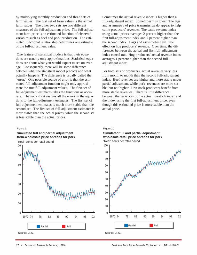
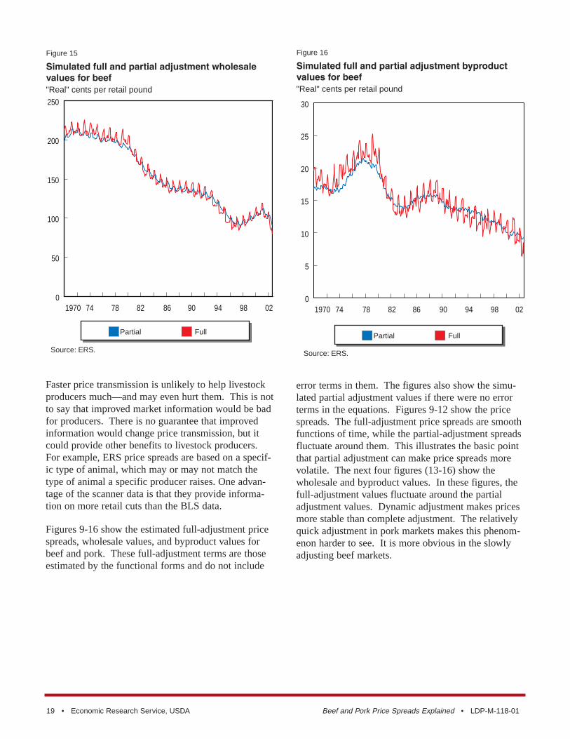
Figures 9-16 show the estimated full-adjustment pricespreads, wholesale values, and byproduct values forbeef and pork. These full-adjustment terms are thoseestimated by the functional forms and do not include

error terms in them. The figures also show the simu-lated partial adjustment values if there were no errorterms in the equations. Figures 9-12 show the pricespreads. The full-adjustment price spreads are smoothfunctions of time, while the partial-adjustment spreadsfluctuate around them. This illustrates the basic pointthat partial adjustment can make price spreads morevolatile. The next four figures (13-16) show thewholesale and byproduct values. In these figures, thefull-adjustment values fluctuate around the partialadjustment values. Dynamic adjustment makes pricesmore stable than complete adjustment. The relativelyquick adjustment in pork markets makes this phenom-enon harder to see. It is more obvious in the slowlyadjusting beef markets.


Simulated full and partial adjustment wholesale values for beef

Figure 15


1970 74 78 82 86 90 94 98 020

50

100

150

200

250

Partial Full

Simulated full and partial adjustment byproduct values for beef

Figure 16


1970 74 78 82 86 90 94 98 020

5

10

15

20

25

30

Partial Full


So, in the beef and pork markets, how much do pricespreads matter? Before answering this question, onemust determine what price spreads are supposed tomeasure. Price spreads are based on farm, wholesale,and retail values for beef and pork. These values meas-ure how much an animal’s meat is worth at variousstages of the farm-to-retail marketing channel. Pricespreads provide a rough measure of the economic effi-ciency of the various segments of the channel.Improved technology that lowers costs can lead tolower price spreads. Improved competition in the mar-ket channels can eliminate monopoly or monopsonyprofits, also improving economic efficiency and lower-ing price spreads. High price spreads dampen thederived demand for livestock, which will lead to somecombination of lower livestock prices and lower live-stock production.

How much do price spreads matter? That depends onwhat time frame one considers. From the long-termperspective, higher price spreads cause lower deriveddemand for livestock, and possibly lower livestockprices. The farm-to-wholesale price spreads haveincreased less rapidly than inflation over the past 30years, while the wholesale-to-retail spread hasincreased more rapidly than inflation. Total, inflation-adjusted price spreads are slightly higher now thanthey were 30 years ago.

The declining, inflation-adjusted farm-to-wholesaleprice spread can be explained by the increased effi-ciency observed in meatpacking. Grocery stores seemto have experienced a decline in overall productivity,which is consistent with the increasing wholesale-to-retail spreads. Higher retail meat margins will lead todeclines in the derived demand for livestock, and maycause lower livestock prices.

The problem with assessing how the change in grocerystore productivity has lowered livestock prices is that

the grocery store meat case is only one of the outletsfor beef and pork. High grocery store costs makeother meat outlets more competitive. The effect ofgrocery store costs on livestock prices depends in parton the share of meat going through the retail meatcase. Given the expanding role of export markets,foodservice, and value-added products, changes in gro-cery store costs probably have less influence on live-stock prices now than they did in the past. Increasesin the wholesale-retail price spread have decreased thederived demand for livestock. It is hard to say if thedeclines in the farm-to-wholesale spreads have beenenough to offset the higher wholesale-to-retail spreads.

From the short-term perspective, price spreads arevolatile, which is consistent with dynamic price adjust-ment. In other words, it takes some time for all theprices to adjust to changes in conditions. Althoughadjustment dynamics make price spreads volatile, theextra time it takes prices to adjust to changes makesthem more stable than if price adjustment were instan-taneous. Price adjustment is also asymmetric, in thatall prices adjust more quickly when they are increasingthan when they are decreasing. While asymmetry andprice adjustment have important effects on month-to-month price changes, it appears that they have littleeffect on the average levels of livestock prices whencalculated over several months. However, dynamicprice adjustment makes livestock prices more stablethan they would be under complete price adjustment.This increased price stability may benefit livestockproducers.

Dynamic adjustment in prices causes dynamic adjust-ment in price spreads as well. Price spread adjustmenthas a significant effect on livestock prices. Whenprice spreads are lower than their full-adjustment val-ues, price spread adjustment leads to lower farmprices, and vice versa.


Summary

Ahearn, Mary, Jet Yee, Eldon Ball, and Rich Nehring,Agricultural Productivity in the United States, AIB-740, ERS-USDA, January 1998.

Food Marketing Institute, Competition and Profit,www.fmi.org/facts_figs/Competitionandprofit.pdf.

Fortune Magazine, electronic edition, “Fortune 500 topperformers”, www.fortune.com/fortune/, accessed June2003.

Gale, Fred, and Maureen Kilkenny, “Agriculture’sRole Shrinks as the Service Economy Expands,” RuralConditions and Trends, Volume 10, Issue 2, ERS-USDA, July 2000.

Gourieroux, J., J. Laffont, and A. Monfort, “CoherencyConditions in Simultaneous Linear Equation Modelswith Endogenous Switching Regimes,” Econometrica,Volume 48, Number 3, April 1980.

Hahn. William F., Asymmetry in Price Transmissionfor Beef and Pork, TB-1769, ERS-USDA, December1989.

Hahn, William F., “Price Transmission Asymmetry inPork and Beef Markets,” Journal of AgriculturalEconomics Research, volume 42, number 4, Fall 1990.

Harris, J. Michael, Phil R. Kaufman, Steve W.Martinez (coordinator), and Charlene Price, The U.S.Food Marketing System: 2002, Competition,Coordination, and Technological Innovations Into the21st Century, AER–811, ERS-USDA, June 2002;

Mathews, Kenneth H., William F. Hahn, Kenneth E.Nelson, Lawrence A. Duewer, and Ronald A.Gustafson, U.S. Beef Industry: Cattle Cycles, PriceSpreads, and Packer Concentration, TB-1874, ERS-USDA, April 1999.

U.S. Department of Agriculture, AgriculturalMarketing Service, 5 Area Weekly Weighted AverageDirect Slaughter Cattle, various issues.

U.S. Department of Agriculture, AgriculturalMarketing Service, National Carlot Meat Report, vari-ous issues.

U.S. Department of Agriculture, AgriculturalMarketing Service, National Daily Base Lean HogCarcass Slaughter Cost, various issues.

U.S. Department of Agriculture, National AgriculturalStatistics Service. Hogs and Pigs (various issues).

U.S. Department of Labor, Bureau of Labor Statistics.Annual Indices of Output Per Hour for SelectedIndustries (various issues).


References

http://www.fmi.org/facts_figs/Competitionandprofit.pdf

http://www.fortune.com/fortune/

This appendix consists of two parts. The first partexamines the theoretical relationship between pricespreads or marketing margins and the derived demandfor livestock. The second part is an econometricmodel of shortrun price interactions among the farm,wholesale, retail, and byproduct values for beef andpork.

Price Spreads and Farm Prices

The goal here is to compare how the farm price reactsto margins in any of the product's potential marketingchannels. We will leave the definition of marketingchannel vague. We will work within a derived demandcontext, and therefore will treat farm production asexogenous. (We will not worry about supply respons-es.) We also treat the margins in the marketing chan-nels as fixed/exogenous. The endogenous variablesare the farm price, the various retail prices, and theamount of farm product going through the variouschannels. The following derivations examine the longrun relationship between marketing costs/marginsand livestock prices. In the long run, we expect highermarketing costs to produce lower farm prices. Short-term price adjustment can make price spreads higherthan their full-adjustment values, which means thatrelatively high price spreads can be a leading indicatorof future increases in livestock prices.

There is one type of farm production, and the level ofthat production is denoted by “q.” This farm productioncan be used to produce an array of retail goods. Thisarray of retail goods will be denoted by the vector “Y.”We are going to assume that the retail prices of the out-puts, denoted by the vector “R,” can be written as thefarm price plus a markup, as in the equation below:

R = f *[1] + M

In (a1), R is the retail price vector, f is the farm price,[1] is a vector of ones, and M is a marketing margin orprice-spread vector. We are measuring retail prices infarm-price-equivalent units. (When calculating beefand pork price spreads, we calculate all the prices inretail-weight equivalent units.) We have assumedaway differences in the animals' cuts in specifying(a1). The pricing implied by (a1) is consistent withconstant-returns-to-scale transformation of retail prod-

ucts from farm products and competitive markets.One need only aggregate all the marketing inputs usedin each sector to a single input for that sector, thenscale the R and M appropriately. The derivative of anyretail price with respect to the farm price is one (1)and the derivative of the retail price with respect to itsinput-cost index is also one (1). Equation (a1) is alsoconsistent with a fixed-proportions technology andfixed markups over the farm price.

Because of the way the retail output is scaled, we canrelate the total farm input used to the retail outputusing the following function:

q = [1]'Y

To complete our system of equations, we are going toassume a set of retail demand functions. The deriva-tives of this system with respect to price (∂Y/∂R) aredenoted by the matrix “D.”

To show the relationship between margins and thefarm price, we create the differential system using thedemand system, (a2) and (a1):

Solving (a3) for the derivatives of its endogenous vari-ables with respect to its exogenous variables gives:

The change in the farm price from a change in one ofthe margins is given by:


Appendix

DI

RYf

IMq

−−

−

=

1 00 1

0 1 0

0 00

0 1

[ ][ ]

[ ]' [ ]' [ ]'

∂∂∂

∂∂

(a3)

∂∂∂

∂∂

RYf

I DD D

D I DD

DD

DD D

Mq

=

−

−

−

[ ]*[ ]'[ ]' [ ]

[ ][ ]' [ ]

[ ]*[ ]'[ ]' [ ]

[ ][ ]' [ ]

[ ]'[ ]' [ ] [ ]' [ ]

1 11 1

11 1

1 11 1

11 1

11 1

11 1

∂∂fM

DD

= −[ ]'[ ]' [ ]1

1 1(a5)

(a2)

(a4)(a1)

Equation (a5) is simply a small part of (a4). We wouldgenerally expect that all the terms of (a5) would benegative because increasing margins should notincrease the farm price. If there is only one outlet forthe farm product, then (a5) implies that increases inthe margin causes an equal decrease in the farm price:

In (a6) “d” is the demand derivative of the single retailoutput with respect to its price. It is a single number,not a block of numbers. Likewise the vector [1] col-lapses to the number 1. In the case with multiple out-lets, if all the margins change by one, then (a5) impliesthat:

We would expect that having one of the marginschange would have a lesser effect on the farm pricethan having all of the margins change. That is, anincrease in one margin is likely to decrease the farmprice by less than the change in the margin.

The effect that a margin change has on the farm pricedepends on all the derivatives of the demand system.Economists seldom work with demand derivatives;they generally work with demand elasticities. Thelarger the demand elasticity, the larger the demandderivative. For a given elasticity, larger quantitiesand/or smaller retail prices make the demand deriva-tives larger. Low margins in a channel mean that itsretail prices are low. The more elastic the demand, thelower the margin, and the larger the volume movingthrough the channel, the larger the effect the channel'smargin has on the derived demand for livestock.

We have not defined the term “marketing channel.”The generic format that we have used so far is consis-tent with many definitions. We could treat each possi-ble way that the animal could get from the farm to anyconsumer as a different channel. For the most part, weare interested in more aggregated definitions of market-ing channels. For purposes of discussion, we will con-sider grocery store markets, the food service group, andthe export market. It is safe to combine these channels

if the individual firms in each of the three sectors havesimilar costs. For example, it makes sense to talkabout a grocery store sector if grocery stores' meatmarkups follow one another closely over time.

Note also that we have not separated out the packingsector from the downstream marketing firms. All ani-mals go through the packing sector before their meatenters the other marketing channels. If we treat meat-packing as a single marketing channel and the whole-sale meat price as a “retail” price, then (a6) becomesrelevant. We expect that a 1-cent increase in the farm-to-wholesale spread would translate into a 1-centdecrease in the farm price.

ERS price spread statistics focus on the farm-to-grocery store part of the marketing system. Equation(a7) implies that a 1-cent increase in the wholesale-retail spread would decrease farm prices by less than 1cent. The exact effect cannot be estimated with cur-rent information. We know that grocery store sales arean important outlet for beef and pork, and grocerystore margins are lower than food service margins butprobably higher than export margins. We do not knowthe own- and cross-price elasticities of demand for thevarious marketing channels' outputs; although wewould expect that export demand would be more elas-tic than the other two channels.

The foodservice and export markets have becomeincreasingly important markets for U.S. meat, whichmeans that the supermarket sector has become lessimportant. This makes the farm-to-retail price spreadhave less of an influence on the derived demand forlivestock.

The derivations above are based on the assumptionthat the price spreads in the different marketing chan-nels are independent. This is unlikely to be the case,especially if the different marketing channels use someof the same nonmeat inputs. We could make the rela-tionship expressed in (a1) more complex by makingthe vector of margins, M, a function of input prices.Changes in the costs of common inputs would lead tochanges in more than one of the elements of M. Pricespread calculations attempt only to measure (at best)total margins, not the contribution of individual inputsto margins.

One special case we could analyze is where the mar-gins in all the markets are proportional to one another.This is the case where if one margin increases by 1percent, all the others also increase by 1 percent. If


∂∂fM

dd

=−

= −1 (a6)

∂ ∂∂

∂f fM

M DD

DD

= = − = − = −* [ ]'[ ]' [ ]

*[ ] [ ]' [ ][ ]' [ ]

11 1

1 1 11 1

1 (a7)

this is the case, we can create a common marketingcost index for all the marketing channels. Call it “s.”Each marketing channel's margin would be “s” timessome constant. The more marketing inputs used, thehigher the constant. We could make “s” equal to thegrocery-store margin and the grocery store's constantequal to 1. A 1-cent increase in the farm-to-retail mar-gin implies a k-cent increase in all the other channels'margins. We can express this relationship using thefollowing function:

M = Ks (a8)

“K” in (a8) is a vector of positive constants.Combining (a8) and (a5) gives us:

It turns out that equation (a9) is uninformative. A 1-cent change in the farm-to-retail margin can be associ-ated with a decrease in derived demand by more orless than 1 cent. We would expect that the decreaseimplied by (a9) in the derived demand for livestock isgreater than that implied by a change in the farm-to-retail margin alone.

The Dynamic Asymmetric Model

The statistical model used in this analysis is anendogenous switching model. This type of model hasbeen used to model price spread behavior by Hahn(1989, 1990) and in Mathews et al. The previousworks were all three-equation systems predictinggross-farm, wholesale, and retail prices, ignoring thebyproduct price. This model predicts all four values.The new model also puts fewer restrictions on howprices interact. The new model uses quadratic splinesto estimate the full-adjustment price spreads, which isa more flexible approach than was used before.

Standard econometric software does not include rou-tines for the estimation of this type of endogenousswitching model. Mathematical programming soft-ware was used. The equation structure may appearodd for three reasons. The first is that the equationsare designed for the convenience of the software. Thesecond is that no prior markup or markdown structurewas imposed on the models. The structure allows thedata to “select” the best type of price-transmissionrelationships. The third reason is that the farm-wholesale and wholesale-retail spread equations aredesigned to directly calculate the full-adjustmentspreads.

The structure of the model makes somewhat moresense if one starts with a general, symmetric, partial-adjustment model, then adds asymmetry to it. A gener-al, symmetric partial adjustment model can be written:

In (b1), dYt is a vector of changes in the four values; Θis a (4 by 4) matrix of adjustment parameters; Tt is avector of target levels for the meat value, byproductvalue, and the two price spreads; At-1 is last month'sactual values; while et is a vector of four random errorterms. The term “target” is generally used in theeconometric literature to mean “full-adjustment.”Since this is the technical appendix, we use the moretechnical language. The target vector is a function ofother variables. Its structure will be discussed later.Equation (b1) is a very general, partial adjustmentmodel. It is possible to restrict Θ so that it impliescomplete adjustment.

Prior expectations on what the bounds of some of theindividual elements of Θ should be are shown in tableB1. If the elements of the Θ matrix are consistentwith these prior expectations, then price adjustment


∂ ∂∂

fds

fM

K DKD

= = −* [ ]'[ ]' [ ]11 1

(a9)

dY T A et t t t= − +−Θ( )1 (b1)

Appendix table B1—Sign expectations for the ΘΘ matrix1

Price adjustment factor

Meat Byproduct Farm-to- Wholesale-to-Endogenous variable wholesale spread retail spread

Gross farm positive positive negative negativeByproduct positive positiveWholesale positive positive negativeRetail positive positive positive

1Blank cells have no “sensible” prior values and could be either positive or negative.

will move prices toward their target values rather thanaway from their target values.

There are four types of target values: meat value,byproduct value, farm-wholesale spread, and whole-sale-retail spread. A 1-cent increase in the target meatvalue will increase the target values for gross-farmvalue, wholesale value, and retail value by 1 cent. Ifthe target meat value is above the actual meat value,dynamic adjustment ought to raise gross-farm, whole-sale, and retail prices. The target meat value is expect-ed to have positive coefficients in the gross-farm,wholesale, and retail parts of the T matrix. We allowthe effect of higher target meat values on currentbyproduct price to be either positive or negative.

The "byproduct" factor in the T matrix is the byprod-uct value. Live animals have byproducts in them aswell as meat. A 1-cent increase in the target byprod-uct value will also increase the target gross-farm valueby one cent. Rising target byproduct values ought toincrease current livestock and byproduct values. Thereare no prior sign constraints on the effect of byprod-uct-value adjustment on wholesale or retail meatprices.

The other two targets are the farm-wholesale andwholesale-retail price spreads. Suppose the targetfarm-wholesale price spread is above the actual pricespread. The farm-wholesale price spread can increaseif farm prices drop, wholesale prices rise, or byproductprices rise. We also expect that higher wholesaleprices caused by widening the farm-wholesale spreadwill lead to higher retail prices. Making the whole-sale-retail spread wider requires lowering the whole-sale price and/or raising the retail price. Lowering thewholesale price because of increasing wholesale-retailspreads ought to lower the gross-farm value as well.

With mathematical programming software one canimpose bounds on coefficients, which was done in thiscase. Imposing these bounds insures that the estimat-ed adjustment directions make sense and it also helpsto insure that the endogenous switching model iscoherent. Gourieroux, Laffont, and Monfort (1980)discuss coherency conditions. A switching equation iscoherent if you can solve it. If an equation is notcoherent, then it may have more than one solution ornone.

Equation (b1) is useful for estimation of symmetricmodels and static models, but not much help for speci-fying asymmetric models. The first step in making

(b1) asymmetric is to transform it by multiplying bothsides by the inverse of Θ, which will be called “B.”

The trick to making (b2) asymmetric is to split thechanges in endogenous variables into two parts, theincreasing part and the decreasing part. The increas-ing part will be called dYup,t and the decreasing partdYdn,t. Explaining the split is easier with a specificexample. Consider the gross farm value. When thegross farm value is increasing, its term in dYup,t is theincrease in the gross farm value and its term in dYdn,tis 0. When the gross farm value is decreasing, its termin dYup,t is 0 and its term in dYdn,t is the decrease inthe gross farm value. The asymmetric version of (b2)is written as:

One way of transforming (b3) back to (b2) is torequire that Bup and Bdn be the same. Also, since Θcan be restricted to imply complete adjustment, the“B” matrices, if symmetric, can also be restricted toimply complete adjustment. The structure in (b2) canbe tested for complete adjustment and asymmetry.

In an endogenous switching model, the coefficientsthat multiply the dY terms switch when one of theterms changes sign. We could also write (b3) in thesame form as (b2), except that there would be 16 ver-sions of the “B” matrix, and the one selected woulddepend on which directions the four values were mov-ing. The 16 different B matrices were inverted in theprogram to insure that all the implied Θ matrices hadsensible elements.

One commonly used model of price discovery is the“markup” model. In markup models, the farm pricechanges first. The wholesale price dynamically adjuststo the farm price and the farm-to-wholesale pricespread. The retail price dynamically adjusts to thewholesale price and the wholesale-to-retail pricespread. In a markup model, the farm price does notreact to price spreads in the short run. One can alsobuild models where the wholesale or retail prices movefirst and the others follow. The strict leader-followermodels imply that one level of the market is the mostimportant center for price discovery. Leader-followermodels are special cases of more general models whereeach price can have a role in price discovery.


B dY B dY T A eup up t dn dn t t t t⋅ + ⋅ = − +−, , 1 (b3)

B dY T A et t t t⋅ = − +−1 (b2)

The problem with a “pure” leader-follower modelwhen analyzing beef and pork price spreads is thatthere are actually two kinds of products being valued:the value of meat and the value of byproducts. Thegross farm value or animal value has both meat andbyproducts in it. The wholesale and retail values areexclusively meat. Obviously, the byproduct value isexclusively byproducts. To make a leader-followermodel in this case, one needs to select two leadingprices and two following prices. The two leadersdetermine meat and byproduct values. One of theprices selected as a leader has to have meat in it, andthe other has to have byproducts in it. As noted above,there are three variables in the model with meat inthem. There are two with byproducts. Picking one ofthe three variables with meat and one of the two withbyproducts, and dropping the livestock-livestock pairgives five models of price leaders/followers.

The asymmetric price leader-follower models weregenerated by restricting the terms of the two “B”matrices. The leader-follower models have a block-recursive structure. The “meat” and byproduct valueequations only have the two leader terms in them. Thewholesale-to-retail spread equations are functions ofonly the retail and wholesale prices, while the farm-to-wholesale equation is a function of the gross farm,byproduct, and wholesale values only. This makes thefollowing prices a markup or markdown from the lead-ing prices.

The target values , Tt, are a function of other variables.The two target spreads are derived from a quadraticspline function. Past models of this type (e.g. Hahn(1989, 1990), Mathews et al.) specified the targetspread using a trend over time. Graphing this type oftarget value over the months gives a straight line overtime. The spline approach is more flexible. It has anintercept and a trend, like previous research, and atrend squared term. To add further flexibility, every 5years, the intercept, trend, and trend-squared termschange. The different spline functions are related:they are required to join at the ends. For example,there is one function that covers 1970-1974 and anoth-er that covers 1975-1980. The 1970 and 1975 func-tions are required to give the same values forDecember 1974 and January 1975. The two functionscan be different in other months. The 1975 and 1980functions match in December 1979 and January 1980,and so on. Although the specification started with 21potential spline coefficients, the joint restrictions allowthese 21 to be reduced to 9 free terms. Inflation was

factored into the model by multiplying the nine freespline terms by the consumer price index, CPI.

The byproduct and meat price equations also have thenine spline terms. In addition, these two equationshave seasonality and depend on beef and pork produc-tion. Seasonality is measured using four harmonicvariables. Beef and pork production get the asymmet-ric treatment also as they are both split into increases,decreases, and last month's values. The seasonal andquantity terms are also multiplied by the CPI toaccount for inflation over the sample.

The last part of the general, asymmetric model thatneeds to be specified is the error term. It is specifiedusing a very general, first-order process:

In (b4), R is a matrix of general autocorrelation effectsand ut is a normally distributed error term with mean 0that is identically and independently distributed overtime. This very general error structure was selected sothat the leader-follower models and the most generalmodel would nest one another.

Estimates and Tests

Table B2 presents the statistical tests for dynamicadjustment and asymmetry. The complete adjustmentand symmetric adjustment models are rejected for bothbeef and pork. Table B3 presents the tests of theasymmetric leader-follower models against the gener-al, asymmetric model. You will note that there are twosets of tests of the leader-follower models in table B3.One set imposes the block-recursive structure only onthe “B” matrices. The other assumed that the errorstructure, including the autocorrelation, was also blockrecursive. One of the indirect implications one mightdraw from the results of table B3 is that allowing verygeneral autocorrelation greatly improves model per-formance. Some models not reported here were runwith more structured autoregressive relationships; free-ing up the autoregression greatly improves model per-formance.

Tables B4 and B5 show the “B” matrix estimates andthe quantity and seasonality estimates for the mostgeneral beef and pork models. Rather than report thespline-coefficient estimates, the splines' effects on thebyproduct and wholesale values for beef and pork aregraphed in figures B1 and B2. The spline effects on


e R e ut t t= ⋅ +−1 (b4)

the price spreads are graphed in the main part of thedocument.

One of the sets of simulations measured the ability ofthe system to explain changes in the prices.Predictions of changes in the gross-farm, byproduct,wholesale, and retail values can be used to make pre-dictions of the net-farm value and spreads. The sym-metric versions of the model are linear, which meansthat the current error terms' mean effect on the values

is zero. Switching and asymmetry make the modelnonlinear, and the average effects of this month's errorterms are not zero. Getting the average error termeffect is a complicated problem involving multinomialprobit analysis, so the simulations estimated median(error terms are 0) predictions. Table B6 shows the fitbetween actual and median values and price spreadsusing r-square as a measure of fit. The r-squares arequite good, given that first-differences in the data arebeing analyzed.


Appendix table B2—Testing hypotheses: dynamics and asymmetry

Species Hypothesis Degrees Likelihood Significance 5% critical of freedom ratio test level value

Beef Adding dynamics to static model 16 226.20 0.00% 26.30 Beef Adding asymmetry to dynamic model 16 37.06 0.21% 26.30 Beef Adding dynamics and asymmetry to static model 32 263.26 0.00% 46.19 Pork Adding dynamics to static model 16 207.05 0.00% 26.30 Pork Adding asymmetry to dynamic model 16 43.34 0.02% 26.30 Pork Adding dynamics and asymmetry to static model 32 250.40 0.00% 46.19

Byproduct spline effects

Figure B1

Cents/pound, retail weight

1970 74 78 82 86 90 94 98 020

20

40

60

80

100

120

pork beef

Meat-price spline effects

Figure B2

Cents/pound, retail weight

1970 74 78 82 86 90 94 98 020

50

100

150

200

250

300

350

400

450

500

pork beef


Appendix table B3—Making the models block recursive: testing uni-directional price transmission

Market determining the values of Degrees Likelihood Significance

Species Meat Byproducts of freedom ratio test level

Testing block recursive model against most general, asymmetric modelBeef farm byproduct 26 312.05 0.00%Beef wholesale farm 26 341.02 0.00%Beef wholesale byproduct 26 315.34 0.00%Beef retail farm 26 833.32 0.00%Beef retail byproduct 26 426.36 0.00%

Pork farm byproduct 26 243.39 0.00%Pork wholesale farm 26 500.45 0.00%Pork wholesale byproduct 26 386.51 0.00%Pork retail farm 26 994.58 0.00%Pork retail byproduct 26 592.58 0.00%

Testing block recursive structure with general covariance and autocorrelationBeef farm byproduct 14 169.32 0.00%Beef wholesale farm 14 76.77 0.00%Beef wholesale byproduct 14 83.05 0.00%Beef retail farm 14 69.87 0.00%Beef retail byproduct 14 57.34 0.00%

Pork farm byproduct 14 141.58 0.00%Pork wholesale farm 14 76.13 0.00%Pork wholesale byproduct 14 26.78 2.06%Pork retail farm 14 53.03 0.00%Pork retail byproduct 14 167.81 0.00%


Appendix table B4—Asymmetry coefficient (B-matrix) estimates1

Item Level Byproduct Farm-to-wholesale Wholesale-to-retail

Beef results:Increase in byproduct value 1.3903 1.9346 0.7420 1.2175Decrease in byproduct value 1.7137 2.2751 0.9868 1.3288Lagged byproduct value 0 1 1 0Increase in gross farm value 2.8873 0.3413 -0.2001 -0.4571Decrease in gross farm value 4.1001 0.7554 -0.0083 0.7442Lagged gross farm value 0 0 -1 0Increase in wholesale value 0.5926 -0.0424 0.8866 -0.8409Decrease in wholesale value 0.0000 -0.2928 0.8155 -1.9445Lagged wholesale value 1 0 1 -1Increase in retail value 1.8114 0.7318 0.1975 3.4206Decrease in retail value 4.4807 1.2191 0.7248 3.8695Lagged retail value 0 0 0 1

Pork results:Increase in byproduct value -1.0615 0.8309 0.9102 0.2371Decrease in byproduct value -1.2554 0.8309 0.0000 0.2804Lagged byproduct value 0 1 1 0Increase in gross farm value -0.0618 0.0484 -1.2072 0.0138Decrease in gross farm value 0.3085 0.0350 -0.9619 -0.0689Lagged gross farm value 0 0 -1 0Increase in wholesale value 1.6143 -0.0315 1.6812 -0.4881Decrease in wholesale value 1.6649 -0.0055 1.8432 -0.3719Lagged wholesale value 1 0 1 -1Increase in retail value 0.6595 0.0057 0.5436 1.3994Decrease in retail value 1.4028 0.0504 0.9187 1.7762Lagged retail value 0 0 0 1

1 Lagged-price coefficients are fixed, not estimated.

Appendix table B5—Quantity and seasonal parameter estimates

Beef estimates Pork estimatesLevel Byproduct Level Byproduct

Seasonal factor 1, cosine 1 turn per year 0.3052 0.0199 -0.5606 -0.0345Seasonal factor 2, cosine 2 turns per year -1.1511 -0.3424 -0.7406 -0.0817Seasonal factor 3, sine 1 turn per year 4.7461 0.5406 0.1980 -0.0501Seasonal factor 4, sine 2 turns per year 2.8960 0.6929 -0.0871 0.0071Increase in beef production (in logarithms) -37.1980 -8.3374 44.1702 2.7463Decrease in beef production (in logarithms) -41.1724 -9.7517 45.6015 2.5708Last month's beef production (in logarithms ) -49.8862 -13.0418 40.1690 2.0163Increase in pork production (in logarithms) 35.2243 7.5408 -55.1258 -3.6281Decrease in pork production (in logarithms) 24.9107 5.4591 -62.1463 -3.8888Last month's pork production (in logarithms) 32.7133 7.1576 -70.5305 -4.3162


Appendix table B6—Measuring the most general models’ median forecast fit using R-squares

Item Beef Pork

PercentGross farm value 36.61 46.64 Byproduct value 25.13 36.64 Net farm value 35.89 46.64 Wholesale value 35.78 34.26 Retail value 57.89 51.53 Farm-to-wholesale price spread 37.80 43.37 Wholesale-to retail price spread 28.63 29.30 Total price spread 32.25 44.48

beef and pork values and price spreads explained

Documents