beams triangular distributed force - kmim.wm.pwr.edu.pl
TRANSCRIPT

Beams – triangular distributed force
Since the theory is best understood by example, below I will introduce a step-by-step solution to
a simple beam with all types of loads. An important information, the beam solution also includes
drawing internal force diagrams.
Ex.6
For the beam shown in the drawing determine: reactions in supports, bending moments, cutting
forces and normal forces. Draw the graphs of these forces. Data: a, F = q*a, q.
1. The first thing to do when solving beams is to determine the number of supporting
unknowns, as was the case with trusses. It is clear that in this case we have three unknown
supports. In addition, you must specify how we will adopt the coordinate system in
accordance with which we will determine the values of supporting unknowns and in which
direction the moments will have positive values. In this case, clockwise turning moments will
be positive.
2. Now we can find the unknown reactions in the supports. In order to do this we will use our
three equations of equilibrium. Of course we cannot forget about assumption that moments
rotating anticlockwise will be with positive sign.
∑ 𝐹𝑥𝑖
𝑛
𝑖=1
= 0; ∑ 𝐹𝑦𝑖
𝑛
𝑖=1
= 0; ∑ 𝑀𝑂
𝑛
𝑖=1
= 0
3. However, before calculating the unknown reactions, I will show you how you can reduce the
force in the case of a triangular load. First of all, as in the case of a rectangular load, we must

calculate the surface area of our figure formed by the distributed load. In this case, a triangle.
Our reduced force will be Q.
4. In the next step, we need to determine where this reduced force is located. In the case of a
rectangle, the matter was simple, because we put the reduced force at the intersection of
the diagonals. In this case, our figure is a triangle. In a right-angled triangle, the reduced
force will always be a third of the distance from the long side and two-thirds from the short
side, as shown in the figure below.
5. Now that we know where the reduced force from the continuous load is, we can calculate
the reactions (we will know the distance needed in the equation of moments).
∑ 𝐹𝑥𝑖
𝑛
𝑖=1
= 0; ∑ 𝐹𝑦𝑖
𝑛
𝑖=1
= 0; ∑ 𝑀𝑂
𝑛
𝑖=1
= 0
∑ 𝐹𝑥𝑖
𝑛
𝑖=1
= 0 = 𝑅𝐴𝑥 → 𝑅𝐴𝑥 = 0
∑ 𝐹𝑦𝑖
𝑛
𝑖=1
= 0 = 𝑅𝐴𝑦 +𝐹
2−
𝑞 ∗ 2𝑎
2→ 𝑅𝐴𝑦 =
𝑞 ∗ 2𝑎
2−
𝑞𝑎
2=
𝑞𝑎
2
∑ 𝑀𝐴
𝑛
𝑖=1
= 0 =𝐹
2∗ 2𝑎 −
𝑞 ∗ 2𝑎
2∗
4
3𝑎 − 𝑀𝐴 → 𝑀𝐴 =
𝑞𝑎
2∗ 2𝑎 −
𝑞 ∗ 2𝑎
2∗
4
3𝑎 = −
1
3𝑞𝑎2

6. Important information. Here it will be shown how one can check if the values of unknown
reactions have been counted well. To do this, select a point on the system through which the
directions of previously found reactions do not pass (the exception is the reaction along the X
axis where it is difficult to make a mistake). After choosing a point - in this case it will be a
point marked as C - you should count the sum of moments relative to this point by inserting
the previously calculated reaction values. After conversion at the end we should get zero. If
the value is different, it means that an error has been made somewhere and the reaction
should be recalculated as well as the test equation.
∑ 𝑀𝐶
𝑛
𝑖=1
=𝐹
2∗ 𝑎 −
𝑞 ∗ 2𝑎
2∗ (𝑎 −
2
3𝑎) − 𝑀𝐴 − 𝑅𝐴𝑌 ∗ 𝑎 → 𝑀𝐴
=𝑞𝑎2
2− 𝑞𝑎 ∗
𝑎
3+
1
3𝑞𝑎2 − 𝑎 ∗
𝑞𝑎
2=
𝑞𝑎2
2∗ (
1
2−
1
3+
1
3−
1
2) = 0
7. After determining the reaction in the supports, in the next step we need to determine how
many cuts the beam needs to be made to be able to solve it. First of all, we forget about the
just introduced coordinate system and how the moment rotate with positive value. From
here, we will use the notation for internal forces that was introduced at the beginning. In this
case, I will show a more complicated version of the calculations for a triangular load, that's
why we enter the beam from the left. Of course you can also enter from the right.
8. Cuts will be made on the beam in places where something happens on the beam (something
appears or disappears). The important information is that we always cut before something
on the beam has happened.

We see that when we enter the beam from its left, forces F/2 and triangular distributed force
appear. However, we cannot make the cut before these forces, because then we are not yet
on the beam. We go further along the beam and come across force RAY and moment MA.
Something happened, force and moment appeared. So we know that in this place just before
the appearance of force RAY and moment MA should be first cut.
9. In this way, we divided the beam into one section I. The first section within 0 ≤ 𝑥 < 2𝑎.
BENDING MOMENTS, CUTTING FORCES, NORMAL FORCES
10. At this point, we can move on to determining internal forces. To do this we have to go
through the section. In this example, at the beginning we will determine what sign will have
the bending moment from each of the forces in our section.
I section within 0 ≤ 𝑥 < 2𝑎.
The bending moment will be from the F/2 force and will look like in the picture (dashed
purple line).
And also the bending moment will be from the triangular distributed force and will look like
in the picture (dashed purple line).

11. In order to overcome the difficulty that is associated with a triangular load in this case, let's
move slightly beyond half the beam. It can be clearly seen that from our triangle load we
have actually got a trapezoid. And this figure is the problem here. Because I know where the
reduced force will be for the rectangle and the triangle, but it is difficult to determine the
position of the reduced force for the trapezoid.
12. To deal with this problem, let's replace our trapezoid with two known triangle and rectangle
figures.
13. We are now introducing a reduced force from each load into our system.
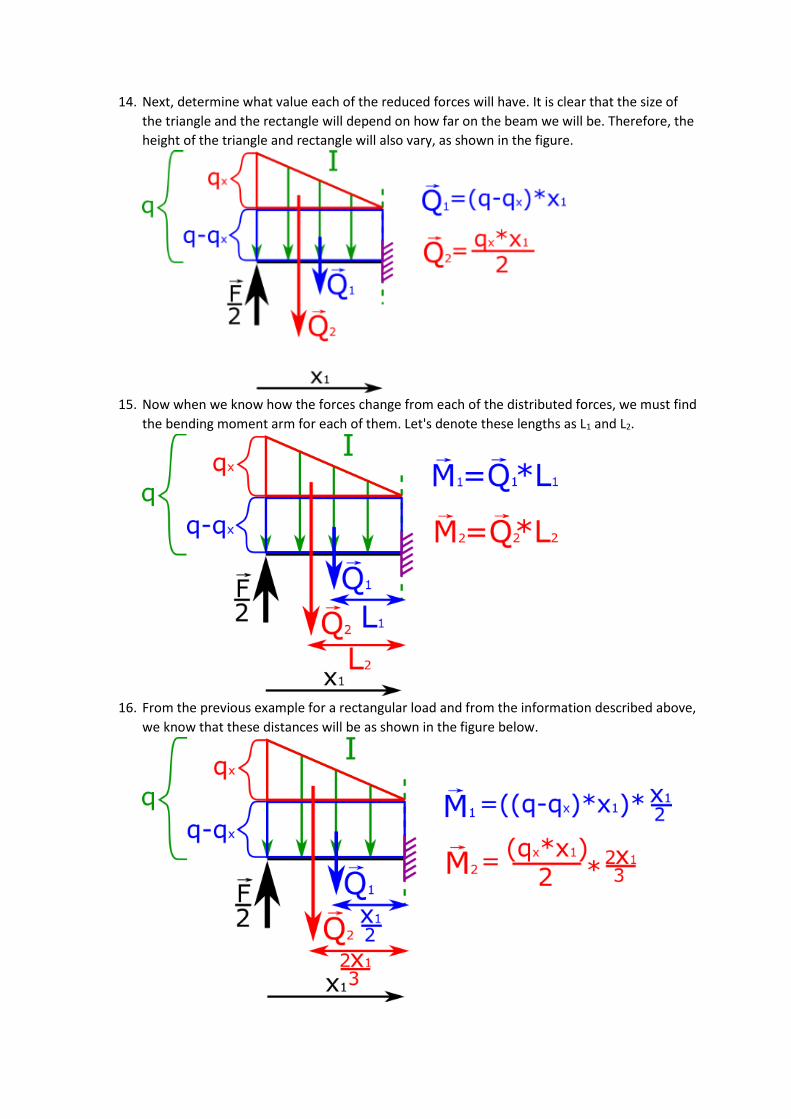
14. Next, determine what value each of the reduced forces will have. It is clear that the size of
the triangle and the rectangle will depend on how far on the beam we will be. Therefore, the
height of the triangle and rectangle will also vary, as shown in the figure.
15. Now when we know how the forces change from each of the distributed forces, we must find
the bending moment arm for each of them. Let's denote these lengths as L1 and L2.
16. From the previous example for a rectangular load and from the information described above,
we know that these distances will be as shown in the figure below.
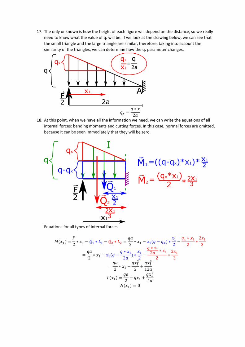
17. The only unknown is how the height of each figure will depend on the distance, so we really
need to know what the value of qx will be. If we look at the drawing below, we can see that
the small triangle and the large triangle are similar, therefore, taking into account the
similarity of the triangles, we can determine how the qx parameter changes.
𝑞𝑥 =𝑞 ∗ 𝑥
2𝑎
18. At this point, when we have all the information we need, we can write the equations of all
internal forces: bending moments and cutting forces. In this case, normal forces are omitted,
because it can be seen immediately that they will be zero.
Equations for all types of internal forces
𝑀(𝑥1) =𝐹
2∗ 𝑥1 − 𝑄1 ∗ 𝐿1 − 𝑄2 ∗ 𝐿2 =
𝑞𝑎
2∗ 𝑥1 − 𝑥1(𝑞 − 𝑞𝑥) ∗
𝑥1
2−
𝑞𝑥 ∗ 𝑥1
2∗
2𝑥1
3
=𝑞𝑎
2∗ 𝑥1 − 𝑥1(𝑞 −
𝑞 ∗ 𝑥1
2𝑎) ∗
𝑥1
2−
𝑞 ∗ 𝑥12𝑎 ∗ 𝑥1
2∗
2𝑥1
3
=𝑞𝑎
2∗ 𝑥1 −
𝑞𝑥12
2+
𝑞𝑥13
12𝑎
𝑇(𝑥1) =𝑞𝑎
2− 𝑞𝑥1 +
𝑞𝑥12
4𝑎
𝑁(𝑥1) = 0

19. Let's write equations for the whole beam in one place to clarify everything.
∑ 𝐹𝑥𝑖
𝑛
𝑖=1
= 0 = 𝑅𝐴𝑥 → 𝑅𝐴𝑥 = 0
∑ 𝐹𝑦𝑖
𝑛
𝑖=1
= 0 = 𝑅𝐴𝑦 +𝐹
2−
𝑞 ∗ 2𝑎
2→ 𝑅𝐴𝑦 =
𝑞 ∗ 2𝑎
2−
𝑞𝑎
2=
𝑞𝑎
2
∑ 𝑀𝐴
𝑛
𝑖=1
= 0 =𝐹
2∗ 2𝑎 −
𝑞 ∗ 2𝑎
2∗
4
3𝑎 − 𝑀𝐴 → 𝑀𝐴 =
𝑞𝑎
2∗ 2𝑎 −
𝑞 ∗ 2𝑎
2∗
4
3𝑎 = −
1
3𝑞𝑎2
I Section 0 ≤ 𝑥1 < 2𝑎
𝑀(𝑥1) =𝐹
2∗ 𝑥1 − 𝑄1 ∗ 𝐿1 − 𝑄2 ∗ 𝐿2 =
𝑞𝑎
2∗ 𝑥1 − 𝑥1(𝑞 − 𝑞𝑥) ∗
𝑥1
2−
𝑞𝑥 ∗ 𝑥1
2∗
2𝑥1
3
=𝑞𝑎
2∗ 𝑥1 − 𝑥1(𝑞 −
𝑞 ∗ 𝑥1
2𝑎) ∗
𝑥1
2−
𝑞 ∗ 𝑥12𝑎
∗ 𝑥1
2∗
2𝑥1
3
=𝑞𝑎
2∗ 𝑥1 −
𝑞𝑥12
2+
𝑞𝑥13
12𝑎
𝑇(𝑥1) =𝑞𝑎
2− 𝑞𝑥1 +
𝑞𝑥12
4𝑎
𝑁(𝑥1) = 0

CHARTS
20. The last part related to solving beams – charts. To easily draw charts, it is best to draw them
under the beam, which we solve, as shown in the figure.

21. In this example, the charts will be drawn for all internal forces.
We will need the equation for the first section.
𝑀(𝑥1) =𝑞𝑎
2∗ 𝑥1 −
𝑞𝑥12
2+
𝑞𝑥13
12𝑎
𝑇(𝑥1) =𝑞𝑎
2− 𝑞𝑥1 +
𝑞𝑥12
4𝑎
𝑁(𝑥1) = 0
We know the limits of the first section.
0 ≤ 𝑥 < 2𝑎
We substitute the boundary values into our equations (for x1).
𝑀(0) =𝑞𝑎
2∗ 0 −
𝑞0
2+
𝑞0
12𝑎= 0
𝑀(2𝑎) =𝑞𝑎
2∗ 2𝑎 −
𝑞(2𝑎)2
2+
𝑞(2𝑎)3
12𝑎= −
𝑞𝑎2
3
𝑇(0) =𝑞𝑎
2− 𝑞0 +
𝑞0
4𝑎=
𝑞𝑎
2
𝑇(2𝑎) =𝑞𝑎
2− 𝑞2𝑎 +
𝑞(2𝑎)2
4𝑎= −
𝑞𝑎
2
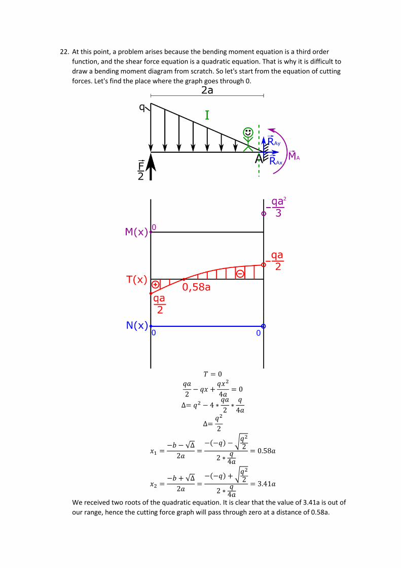
22. At this point, a problem arises because the bending moment equation is a third order
function, and the shear force equation is a quadratic equation. That is why it is difficult to
draw a bending moment diagram from scratch. So let's start from the equation of cutting
forces. Let's find the place where the graph goes through 0.
𝑇 = 0
𝑞𝑎
2− 𝑞𝑥 +
𝑞𝑥2
4𝑎= 0
∆= 𝑞2 − 4 ∗𝑞𝑎
2∗
𝑞
4𝑎
∆=𝑞2
2
𝑥1 =−𝑏 − √∆
2𝑎=
−(−𝑞) − √𝑞2
2
2 ∗𝑞
4𝑎
= 0.58𝑎
𝑥2 =−𝑏 + √∆
2𝑎=
−(−𝑞) + √𝑞2
2
2 ∗𝑞
4𝑎
= 3.41𝑎
We received two roots of the quadratic equation. It is clear that the value of 3.41a is out of
our range, hence the cutting force graph will pass through zero at a distance of 0.58a.

23. Knowing where the cutting force graph goes through zero and that the shear force graph is a
derivative of the bending moment, we can say that the bending moment function must take
the extreme here. Therefore, the bending moment value for this distance should be
calculated.
𝑀(0.58𝑎) =𝑞0.58𝑎
2∗ 2𝑎 −
𝑞(0.58𝑎)2
2+
𝑞(0.58𝑎)3
12𝑎= 0,138 𝑞𝑎2
In addition, it is also worth calculating the value for half the section.
𝑀(𝑎) =𝑞𝑎
2∗ 2𝑎 −
𝑞(𝑎)2
2+
𝑞(𝑎)3
12𝑎=
1
12𝑎 𝑞𝑎2