beam element in fem/fea
DESCRIPTION
Beam element in FEA/FEM .TRANSCRIPT

Ananthasuresh, IISc
Chapter 7
Finite Element Formulations for Beams and Frames
Beams and frames can take axial, transverse (i.e., perpendicular to the axis), and moment loads. Unlike
truss elements, they undergo bending. In this chapter, we will obtain element stiffness matrix and force
vectors for a beam element by following the same procedure as the one used for the axially loaded bars.
This will reinforce our understanding of the finite element formulation so that we can discuss the general
procedure for any type of element in the coming chapters.
We will first obtain an expression for the strain energy and work potential of a beam. Then, by
assuming shape functions of certain form, we will write the strain energy for a beam element in order to
obtain the stiffness matrix and force vectors for the element.
7.1 The bending strain energy for a beam
For a beam of length L, we write the strain energy density (= half of the product of stress and strain), and
then integrate it over the entire volume to get SE of the beam.
( )( ) ( ) dVstressE
dVstrainstressSEVV
2
21
21
∫∫ == (1a)
dVI
MyEV
2
21
∫ ⎟⎠⎞
⎜⎝⎛= (1b)
dxdAyEIM
L A∫ ∫ ⎪⎭
⎪⎬⎫
⎪⎩
⎪⎨⎧
⎟⎟⎠
⎞⎜⎜⎝
⎛= 2
2
2
2 (1c)
Equation (1b) is obtained by using the fact that the bending stress in a beam is given by
I
Mystress = (2)
Next, we evaluate the area integral in Equation (1c).
⎟⎟⎠
⎞⎜⎜⎝
⎛=⎟⎟
⎠
⎞⎜⎜⎝
⎛=⎟⎟
⎠
⎞⎜⎜⎝
⎛=⎟⎟
⎠
⎞⎜⎜⎝
⎛∫∫ EI
MIEIMdAy
EIMdAy
EIM
AA 2222
2
2
22
2
22
2
2
(3)

7.2
In Equation (3) above, we noticed that IdAyA
=∫ 2 is nothing but the area moment of inertia of the beam
cross-section. Next we use Bernoulli’s beam deflection theorem that states that the bending moment is
proportional to the curvature. Since for small strains, the curvature is given by the second derivative of
the transverse deflection v(x) of the neutral axis, we write:
2
2
dxvdEIM = (4)
Substitution of Equation (3) into Equation (1c) and using (4) yields
dxEI
MSEL∫= 2
2
(5a)
dxdx
vdEIdxdx
vdEIEI LL
2
2
22
2
2
221
⎟⎟⎠
⎞⎜⎜⎝
⎛=⎟⎟
⎠
⎞⎜⎜⎝
⎛= ∫∫ (5b)
The importance of Equation (5b) lies in the fact that if we know the transverse deflection v(x), we can
compute the bending strain energy by evaluating the integral⎯an essential feature for the finite element
formulation.
7.2 Shape functions for beam elements
The first step in the finite element formulation is to choose the suitable shape functions. We will consider
two-noded beam elements. Each node will have three degrees of freedom, viz. axial and transverse
displacements, and the slope. We will first consider only the transverse displacement and the slope, and
we include consider the axial displacement later. We do this because, in bar elements we already
accounted for the axial displacement. It will be a simple matter to include this effect later, as you will see
at the end of this chapter.
x1
x2
ξ=-1 ξ=1ξ
q1q2q3q4
Figure 1 The four degrees of freedom of a beam element in local coordinate system

7.3
The degrees of freedom q1, q2, q3, and q4 are shown in the local ξ -coordinate system in Figure 1.
Recall that the purpose of using a local coordinate system is to make the derivation general so that the
formulation is applicable to all elements of different sizes and orientations. Recall also the transformation
from the local to the global system:
( ) 121 −−= xx
Le
ξ (6)
We will now define four shape functions Ni (i = 1,2,3, and 4) such that v(x) and dx
xdv )(give the transverse
displacement and the slope of the beam respectively.
⎪⎪⎭
⎪⎪⎬
⎫
⎪⎪⎩
⎪⎪⎨
⎧
⎭⎬⎫
⎩⎨⎧=
4
3
2
1
4321 22)(
qqqq
NL
NNL
Nv eeξ (7)
where
( ) ( )
( ) ( )
( ) ( )
( ) ( )1141
2141
1141
2141
24
23
22
21
−+=
−+=
+−=
+−=
ξξ
ξξ
ξξ
ξξ
N
N
N
N
(8)
Note that
dxd
ddv
dxdv ξ
ξξ )(
= (9)
where
eLdxd 2
=ξ
(10)
and
⎪⎪⎭
⎪⎪⎬
⎫
⎪⎪⎩
⎪⎪⎨
⎧
⎭⎬⎫
⎩⎨⎧
=
4
3
2
1
4321
22qqqq
ddN
ddNL
ddNL
ddN
ddv ee
ξξξξξ (11a)
Displacement at node 1
Slope at node 1
Displacement at node 2
Slope at node 2

7.4
⎪⎪⎭
⎪⎪⎬
⎫
⎪⎪⎩
⎪⎪⎨
⎧
⎭⎬⎫
⎩⎨⎧
=
4
3
2
1
24
2
23
2
22
2
21
2
2
2
22qqqq
dNd
dNdL
dNdL
dNd
dvd ee
ξξξξξ (11b)
-1 0 1
0
0.5
1
N1
-1 0 1
-0.5
0
0.5
N2
-1 0 1
0
0.5
1
N3
-1 0 1
-0.5
0
0.5
N4
Figure 2 Plots of beam shape functions
We should pause a little here to think about why the shape functions are defined this way. Study
Figure 2 carefully where the four shape functions are shown graphically. Note that N1 has zero slope at
the beginning and end, and zero value at the end. Likewise, N2 has zero values at beginning and the end,
and zero slope at the end. Just as N1 has unit displacement at the beginning, N2 has unit slope (angle =
45°). N3 and N4 exhibit similar features. i.e., i th shape function is zero at all other dofs and unity at i th
dof. Recall from our discussion of shape functions for the bar element. There, the two shape functions
were defined such that each shape function is unity only at one at one end and zero at the other. This is to
ensure that the interpolating shape functions satisfy the deformations at the ends. Here also, all the four

7.5
end conditions q1, q2, q3, and q4 are satisfied, as can be seen in plots in Figure 2. Notice that each shape
function is unity at its corresponding degree of freedom while it is zero at the other degrees of freedom. If
you understand this property, you can easily sketch the shape functions without looking at their
expressions. Please also note that you can also easily derive them then. Let us demonstrate that with the
first shape function.
Shape function )(1 ξN must satisfy four conditions:
0)1(
0)1(
0)1(
1)1(
1
1
1
1
==
==
=−=
=−=
ξξ
ξ
ξξ
ξ
ddNNddNN
(12)
A polynomial curve that satisfies four conditions must be a cubic at the minimum. So, let us take )(1 ξN
to be a cubic in ξ .
33
22101 )( ξξξξ aaaaN +++= (13a)
Then,
2321
1 32)(
ξξξξ
aaad
dN++= (13b)
Conditions in Equation (12) when substituted into Equation (13a) and (13b) give:
0321
0321
321
3210
321
3210
=++=+++
=+−=−+−
aaaaaaa
aaaaaaa
(14)
Solving for 3210 and,,, aaaa in Equation (14) yields
4/1and,0,4/3,5.0 3210 ==−== aaaa
That means
( )331 32
41
41
435.0 ξξξξ +−=+−=N (15)

7.6
You can easily verify that the first shape function in Equation (8a) is the same as the one in Equation (15)
because ( )32 3241)2()1(
41 ξξξξ +−=+− .
It is important to notice also that the shape functions N2 and N4 are multiplied by Le
2. This is
because these two shape functions multiply with slope coordinates which have radians as units. So, this is
necessary in order to be consistent with units in Equation (7). Another reason becomes apparent from
Equations (10) and (11) if you think about the slope being equal to unity at those degrees of freedom.
There is a name to the four shape functions that we just used. They are called Hermite
polynomials. Recall that the shape functions used for bar elements were called Lagrange polynomials.
While Lagrange polynomials satisfy only the C0 continuity (i.e., only the position continuity), Hermite
polynomials satisfy C1 continuity (i.e., the slope is also continuous). In beam elements, since the slope is
one degree of freedom, we need slope continuity.
7.3 Element stiffness matrix for beam elements
As shown in Equation (5b), the strain energy of a beam element is given by
dxdx
vdEISEx
xe ∫ ⎟⎟
⎠
⎞⎜⎜⎝
⎛=
2
1
2
2
2
21
(16)
Using the shape functions and the ξ -coordinate system presented above,
ξ
ξ
ξξ
ξ
ξξ
ξ
ddx
vdLEI
dL
LdxvdEI
dddx
dxd
dxvdEI
dddx
dxd
dxvdEISE
e
e
e
e
∫
∫
∫
∫
−
−
−
−
⎟⎟⎠
⎞⎜⎜⎝
⎛⎟⎟⎠
⎞⎜⎜⎝
⎛=
⎟⎟⎠
⎞⎜⎜⎝
⎛⎟⎟⎠
⎞⎜⎜⎝
⎛=
⎟⎠⎞
⎜⎝⎛
⎟⎟⎠
⎞⎜⎜⎝
⎛=
⎟⎟⎠
⎞⎜⎜⎝
⎛⎟⎟⎠
⎞⎜⎜⎝
⎛⎟⎠⎞
⎜⎝⎛=
1
1
2
2
2
3
1
1
42
2
2
1
1
42
2
2
1
1
22
2
2
821
22
2
2
2
(17)
where 2
2
dxvd
is given in Equation (11b). To evaluate
2
2
2
⎟⎟⎠
⎞⎜⎜⎝
⎛dx
vd, we will use the matrix notation instead of
doing that tediously by expanding Equation (11b). Because squaring a matrix entity is equivalent to
multiplying its transpose with itself,
7.7
⎪⎪⎭
⎪⎪⎬
⎫
⎪⎪⎩
⎪⎪⎨
⎧
⎪⎪⎭
⎪⎪⎬
⎫
⎪⎪⎩
⎪⎪⎨
⎧
⎭⎬⎫
⎩⎨⎧
×
⎪⎪⎭
⎪⎪⎬
⎫
⎪⎪⎩
⎪⎪⎨
⎧
⎪⎪⎭
⎪⎪⎬
⎫
⎪⎪⎩
⎪⎪⎨
⎧
⎭⎬⎫
⎩⎨⎧
=⎟⎟⎠
⎞⎜⎜⎝
⎛⎟⎟⎠
⎞⎜⎜⎝
⎛=⎟⎟
⎠
⎞⎜⎜⎝
⎛
4
3
2
1
24
2
23
2
22
2
21
2
4
3
2
1
24
2
23
2
22
2
21
2
2
2
2
22
2
2
22
22
qqqq
dNdL
dNd
dNdL
dNd
qqqq
dNdL
dNd
dNdL
dNd
dxvd
dxvd
dxvd
ee
T
eeT
ξξξξ
ξξξξ
(18)
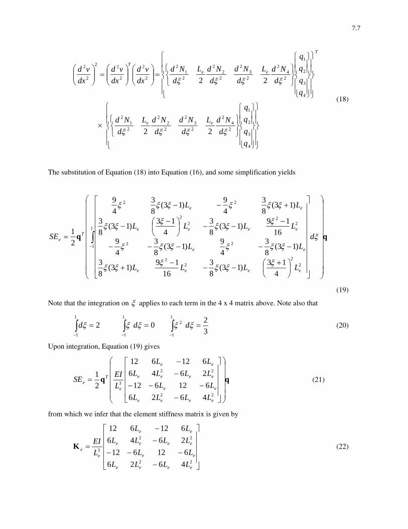
The substitution of Equation (18) into Equation (16), and some simplification yields
⎟⎟⎟⎟⎟⎟⎟⎟⎟⎟
⎠
⎞
⎜⎜⎜⎜⎜⎜⎜⎜⎜⎜
⎝
⎛
⎥⎥⎥⎥⎥⎥⎥⎥⎥
⎦
⎤
⎢⎢⎢⎢⎢⎢⎢⎢⎢
⎣
⎡
⎟⎠⎞
⎜⎝⎛ +
−−−
+
−−−−−
−−−⎟
⎠⎞
⎜⎝⎛ −
−
+−−
= ∫−
1
1
22
22
22
22
22
22
413)13(
83
1619)13(
83
)13(83
49)13(
83
49
1619)13(
83
413)13(
83
)13(83
49)13(
83
49
21 ξ
ξξξξξξ
ξξξξξξ
ξξξξξξ
ξξξξξξ
d
LLLL
LL
LLLL
LL
SE
eeee
ee
eeee
ee
Te
(19)
Note that the integration on ξ applies to each term in the 4 x 4 matrix above. Note also that
∫−
=1
1
2ξd ∫−
=1
1
0ξξ d ∫−
=1
1
2
32ξξ d (20)
Upon integration, Equation (19) gives
⎟⎟⎟⎟⎟
⎠
⎞
⎜⎜⎜⎜⎜
⎝
⎛
⎥⎥⎥⎥
⎦
⎤
⎢⎢⎢⎢
⎣
⎡
−−−−
−−
=
22
22
3
4626612612
2646612612
21
eeee
ee
eeee
ee
e
Te
LLLLLL
LLLLLL
LEISE (21)
from which we infer that the element stiffness matrix is given by
⎥⎥⎥⎥
⎦
⎤
⎢⎢⎢⎢
⎣
⎡
−−−−
−−
=
22
22
3
4626612612
2646612612
eeee
ee
eeee
ee
ee
LLLLLL
LLLLLL
LEIK (22)

7.8
If we also account for axial deformations, and consider a beam with six degrees of freedom as
shown in Figure 3, we get the beam element in the local ξ -coordinate system. We denote this with
“prime” because it is in the local coordinate system. The element stiffness matrix for this case is given by
⎥⎥⎥⎥⎥⎥⎥⎥⎥⎥⎥⎥⎥⎥⎥
⎦
⎤
⎢⎢⎢⎢⎢⎢⎢⎢⎢⎢⎢⎢⎢⎢⎢
⎣
⎡
−
−−−
−
−
−
−
=′
eeee
eeee
e
ee
e
ee
eeee
eeee
e
ee
e
ee
e
LEI
LEI
LEI
LEI
LEI
LEI
LEI
LEI
LEA
LEA
LEI
LEI
LEI
LEI
LEI
LEI
LEI
LEI
LEA
LEA
460260
61206120
0000
260460
61206120
0000
22
2323
22
2323
K (23)
q2q3q5q6
q1 q4
Figure 3 The six degree-of-freedom beam element
Note how we combined the 2 x 2 matrix of the axial stiffness
⎥⎥⎥⎥
⎦
⎤
⎢⎢⎢⎢
⎣
⎡
−
−
e
ee
e
ee
e
ee
e
ee
LEA
LEA
LEA
LEA
, with the 4 x 4
bending stiffness of Equation (23), into a general 6 x 6 matrix in Equation (23). It simply means that
q K qTe will give the sum of axial and bending energies.
In general, an element of a curved beam can be in any orientation. So, we need to derive the
transformation matrix L, as we did in the case of trusses. Refer to Figure 4 and Equation (24) below.

7.9
q2
q3=q'3
q5
q6=q'6
q1
q4
q'1q'2
q'4
q'5
Slope of the element = θ
Figure 4 Arbitrarily oriented beam element
⎪⎪⎪⎪
⎭
⎪⎪⎪⎪
⎬
⎫
⎪⎪⎪⎪
⎩
⎪⎪⎪⎪
⎨
⎧
⎥⎥⎥⎥⎥⎥⎥⎥
⎦
⎤
⎢⎢⎢⎢⎢⎢⎢⎢
⎣
⎡
−
−
=
⎪⎪⎪⎪
⎭
⎪⎪⎪⎪
⎬
⎫
⎪⎪⎪⎪
⎩
⎪⎪⎪⎪
⎨
⎧
1
1
1
1
1
1
1
1
1
1
1
1
1000000000000000010000000000
''''''
qqqqqq
lmml
lmml
qqqqqq
(24)
Now, the stiffness matrix for a six degree-of-freedom beam element is:
LKLK eT
e ′= (21)
This follows from the strain-energy argument that
LqKLqqKq eTT
eT
eSE ′=′=21
21
(22)
7.4 Element force vector for beam elements
The general procedure for deriving the element force vectors was described in Section 5.2 in the context
of bar elements. We will repeat the same here briefly for beam elements with body force f per unit length.
As in Equation (7) of Chapter 5, we write the work potential due f on the element as
qf Te
ee
L
ee
qqqq
dNL
NNL
NfL
dxxvfWP =
⎪⎪⎭
⎪⎪⎬
⎫
⎪⎪⎩
⎪⎪⎨
⎧
⎟⎟⎠
⎞⎜⎜⎝
⎛
⎭⎬⎫
⎩⎨⎧== ∫∫
−
4
3
2
11
14321 222
)( ξ (23)
After performing the integration in matrix form, we get

7.10
⎭⎬⎫
⎩⎨⎧
−=122122
22eeee
efLfLfLfL
f (24)
The force vector due to the distributed surface (or line) force is done in a similar manner. The point forces
and moments are directly included in the global system force vector. It is then necessary to create nodes at
all the locations that have point forces.
7.5 Solving beam FEM problems
The assembly of the global system, imposing the boundary conditions, and all the post-processing
operations are exactly the same as we did for the trusses. Now, we realize the procedure we followed in
the previous chapters is general enough to apply to other types of elements. The only thing that is
different about different elements are the shape functions and the stress-strain and strain energy
relationships. We will discuss the stress-strain relationships in Chapter 8. In the remaining section of this
chapter, we will present the Matlab script for beam FEM problems. Study this script carefully and note
the similarities (and some differences) between this script and the one for truss elements.
7.6 Matlab script for beam FEM
Four input files are needed for beam.m. These files contain the geometric, physical and materiel property,
and force information about the truss to be analyzed.
1) node.dat

7.11
This file contains the (X,Y) coordinates of all the node numbers in the following format.
Node# X-coordinate Y-Coordinate
1 2 3 etc.
2) elem.dat
This file contains the element information pertaining to the two nodes that form the element, the cross-
section area and Young’s modulus of the element.
Element# Node#1 Node#2 Area Young’s modulus Inertia 1 2 3 etc.
3) forces.dat
This file contains the nodal forces to be applied on the truss. You need to specify the node number, the
degree-of-freedom (dof) number (1 if force is in the X-direction, and 2 if the force is in the Y-direction),
and the value of the force. If you have forces in the X and Y directions at the same node, then you need to
put in two lines in the force, one for each direction.
Serial# Node# dof# Force value 1 2 etc.
4) disp.dat
This file contains the information about the displacement boundary conditions, i.e. which nodes and dof’s
are fixed to be zero. dof# is to be treated in the same way as you do in the case of force specification.
Serial# Node# dof# 1 2 etc. ____________________________________ Matlab Scripts for beam FEM
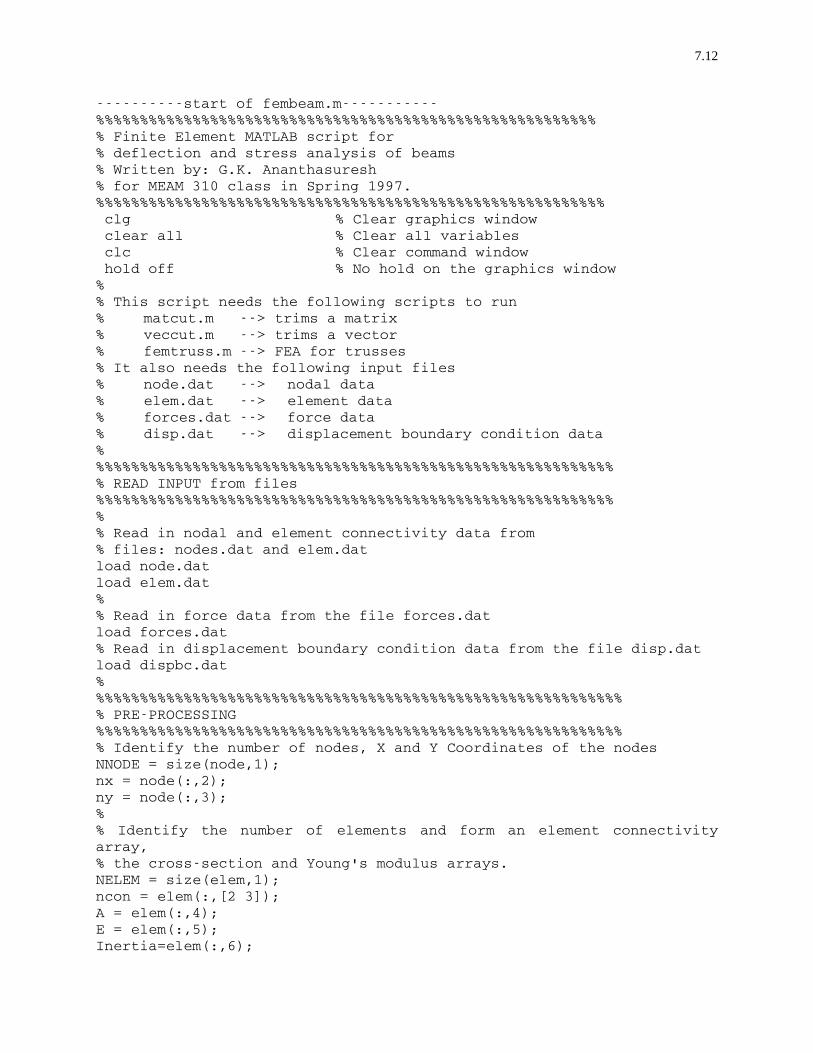
7.12
----------start of fembeam.m----------- %%%%%%%%%%%%%%%%%%%%%%%%%%%%%%%%%%%%%%%%%%%%%%%%%%%%%%%%% % Finite Element MATLAB script for % deflection and stress analysis of beams % Written by: G.K. Ananthasuresh % for MEAM 310 class in Spring 1997. %%%%%%%%%%%%%%%%%%%%%%%%%%%%%%%%%%%%%%%%%%%%%%%%%%%%%%%%%% clg % Clear graphics window clear all % Clear all variables clc % Clear command window hold off % No hold on the graphics window % % This script needs the following scripts to run % matcut.m --> trims a matrix % veccut.m --> trims a vector % femtruss.m --> FEA for trusses % It also needs the following input files % node.dat --> nodal data % elem.dat --> element data % forces.dat --> force data % disp.dat --> displacement boundary condition data % %%%%%%%%%%%%%%%%%%%%%%%%%%%%%%%%%%%%%%%%%%%%%%%%%%%%%%%%%%% % READ INPUT from files %%%%%%%%%%%%%%%%%%%%%%%%%%%%%%%%%%%%%%%%%%%%%%%%%%%%%%%%%%% % % Read in nodal and element connectivity data from % files: nodes.dat and elem.dat load node.dat load elem.dat % % Read in force data from the file forces.dat load forces.dat % Read in displacement boundary condition data from the file disp.dat load dispbc.dat % %%%%%%%%%%%%%%%%%%%%%%%%%%%%%%%%%%%%%%%%%%%%%%%%%%%%%%%%%%%% % PRE-PROCESSING %%%%%%%%%%%%%%%%%%%%%%%%%%%%%%%%%%%%%%%%%%%%%%%%%%%%%%%%%%%% % Identify the number of nodes, X and Y Coordinates of the nodes NNODE = size(node,1); nx = node(:,2); ny = node(:,3); % % Identify the number of elements and form an element connectivity array, % the cross-section and Young's modulus arrays. NELEM = size(elem,1); ncon = elem(:,[2 3]); A = elem(:,4); E = elem(:,5); Inertia=elem(:,6);

7.13
% % Arrange force information into a force vector, F F = zeros(3*NNODE,1); % Initialization Nforce = size(forces,1); for i = 1:Nforce, dof = (forces(i,2)-1)*3 + forces(i,3); F(dof) = forces(i,4); end % % Displacement boundary conditions Nfix = size(dispbc,1); j = 0; for i = 1:Nfix, j = j + 1; dispID(j) = (dispbc(i,2)-1)*3+dispbc(i,3); end dispID = sort(dispID); % % Compute the lengths of the elements for ie=1:NELEM, eye = ncon(ie,1); jay = ncon(ie,2); L(ie) = sqrt ( (nx(jay) - nx(eye))^2 + (ny(jay) - ny(eye))^2 ); end % % %%%%%%%%%%%%%%%%%%%%%%%%%%%%%%%%%%%%%%%%%%%%%%%%%%%%%%%%%%%% % SOLUTION %%%%%%%%%%%%%%%%%%%%%%%%%%%%%%%%%%%%%%%%%%%%%%%%%%%%%%%%%%%% % Call fembeam.m to solve for the following. % Deflections: U % Reaction forces at the constrained nodes: R % Internal forces in each truss member: Fint % Global stiffness matrix: Kglobal % Strain energy: SE fembeam(A,L,E,nx,ny,ncon,NELEM,NNODE,F,dispID,Inertia); % % %%%%%%%%%%%%%%%%%%%%%%%%%%%%%%%%%%%%%%%%%%%%%%%%%%%%%%%%%%%% % POST-PROCESSING %%%%%%%%%%%%%%%%%%%%%%%%%%%%%%%%%%%%%%%%%%%%%%%%%%%%%%%%%%%% % Plotting clg for ip=1:NELEM, pt1 = ncon(ip,1); pt2 = ncon(ip,2); dx1 = U(3*(pt1-1)+1); dy1 = U(3*(pt1-1)+2); dx2 = U(3*(pt2-1)+1); dy2 = U(3*(pt2-1)+2); % plot([nx(pt1) nx(pt2)], [ny(pt1) ny(pt2)],'--c'); hold on

7.14
plot([nx(pt1) nx(pt2)], [ny(pt1) ny(pt2)],'.w'); plot([nx(pt1)+dx1 nx(pt2)+dx2], [ny(pt1)+dy1 ny(pt2)+dy2],'-y'); plot([nx(pt1)+dx1 nx(pt2)+dx2], [ny(pt1)+dy1 ny(pt2)+dy2],'.w'); hold on end xlabel('X'); ylabel('Y'); axis('equal'); ----------end of beam.m----------- ----------start of mcut.m----------- function D = mcut(C,i) % To remove ith row and ith column from C (size: NxN) and % return D (size: N-1xN-1) [m,n] = size(C); d1 = C(1:i-1,1:i-1); d2 = C(1:i-1,i+1:n); d3 = C(i+1:m,1:i-1); d4 = C(i+1:m,i+1:n); D = [d1 d2; d3 d4]; ----------end of mcut.m----------- ----------start of veccut.m----------- function D = veccut(C,i) % To remove member i from C and return D with size 1 less. [m,n] = size(C); if m == 1 d1 = C(1:i-1); d2 = C(i+1:n); D = [d1 d2]; end if n == 1 d1 = C(1:i-1); d2 = C(i+1:m); D = [d1; d2]; end ----------end of veccut.m----------- ----------start of fembeam.m----------- %%%%%%%%%%%%%%%%%%%%%%%%%%%%%%%%%%%%%%%%%%%%%% % This m-file forms the finite element model of a beam % system and solves it. % G.K. Ananthasuresh for MEAM 310 class in Spring 1997. % Inputs: % Ae --> A vector containing the cross-section areas of all % the elements % Le --> A vector containing the lengths of all the elements % Ee --> A vector containing the Young's moduli of all the % elements
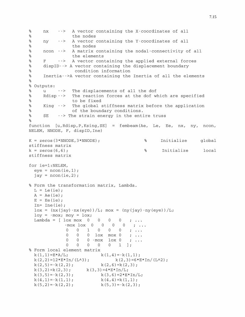
7.15
% nx --> A vector containing the X-coordinates of all % the nodes % ny --> A vector containing the Y-coordinates of all % the nodes % ncon --> A matrix containing the nodal-connectivity of all % the elements % F --> A vector containing the applied external forces % dispID--> A vector containing the displacement boundary % condition information % Inertia-->A vector containing the Inertia of all the elements % % Outputs: % u --> The displacements of all the dof % Rdisp --> The reaction forces at the dof which are specified % to be fixed % King --> The global stiffness matrix before the application % of the boundary conditions. % SE --> The strain energy in the entire truss % function [u,Rdisp,P,Ksing,SE] = fembeam(Ae, Le, Ee, nx, ny, ncon, NELEM, NNODE, F, dispID,Ine) K = zeros(3*NNODE,3*NNODE); % Initialize global stiffness matrix k = zeros(6,6); % Initialize local stiffness matrix for ie=1:NELEM, eye = ncon(ie,1); jay = ncon(ie,2); % Form the transformation matrix, Lambda. L = Le(ie); A = Ae(ie); E = Ee(ie); In= Ine(ie); lox = (nx(jay)-nx(eye))/L; mox = (ny(jay)-ny(eye))/L; loy = -mox; moy = lox; Lambda = [ lox mox 0 0 0 0 ; ... -mox lox 0 0 0 0 ; ... 0 0 1 0 0 0 ; ... 0 0 0 lox mox 0 ; ... 0 0 0 -mox lox 0 ; ... 0 0 0 0 0 1 ]; % Form local element matrix k(1,1)=E*A/L; k(1,4)=-k(1,1); k(2,2)=12*E*In/(L^3); k(2,3)=6*E*In/(L^2); k(2,5)=-k(2,2); k(2,6)=k(2,3); k(3,2)=k(2,3); k(3,3)=4*E*In/L; k(3,5)=-k(2,3); k(3,6)=2*E*In/L; k(4,1)=-k(1,1); k(4,4)=k(1,1); k(5,2)=-k(2,2); k(5,3)=-k(2,3);

7.16
k(5,5)=k(2,2); k(5,6)=-k(2,3); k(6,2)=k(2,3); k(6,3)=k(3,6); k(6,5)=-k(2,3); k(6,6)=k(3,3); klocal = Lambda' * k * Lambda; % Form ID matrix to assemble klocal into the global stiffness matrix, K. id1 = 3*(eye-1) + 1; id2 = id1 + 1; id3 = id2 + 1; id4 = 3*(jay-1) + 1; id5 = id4 + 1; id6 = id5 + 1; K(id1,id1) = K(id1,id1) + klocal(1,1); K(id1,id2) = K(id1,id2) + klocal(1,2); K(id1,id3) = K(id1,id3) + klocal(1,3); K(id1,id4) = K(id1,id4) + klocal(1,4); K(id1,id5) = K(id1,id5) + klocal(1,5); K(id1,id6) = K(id1,id6) + klocal(1,6); K(id2,id1) = K(id2,id1) + klocal(2,1); K(id2,id2) = K(id2,id2) + klocal(2,2); K(id2,id3) = K(id2,id3) + klocal(2,3); K(id2,id4) = K(id2,id4) + klocal(2,4); K(id2,id5) = K(id2,id5) + klocal(2,5); K(id2,id6) = K(id2,id6) + klocal(2,6); K(id3,id1) = K(id3,id1) + klocal(3,1); K(id3,id2) = K(id3,id2) + klocal(3,2); K(id3,id3) = K(id3,id3) + klocal(3,3); K(id3,id4) = K(id3,id4) + klocal(3,4); K(id3,id5) = K(id3,id5) + klocal(3,5); K(id3,id6) = K(id3,id6) + klocal(3,6); K(id4,id1) = K(id4,id1) + klocal(4,1); K(id4,id2) = K(id4,id2) + klocal(4,2); K(id4,id3) = K(id4,id3) + klocal(4,3); K(id4,id4) = K(id4,id4) + klocal(4,4); K(id4,id5) = K(id4,id5) + klocal(4,5); K(id4,id6) = K(id4,id6) + klocal(4,6); K(id5,id1) = K(id5,id1) + klocal(5,1); K(id5,id2) = K(id5,id2) + klocal(5,2); K(id5,id3) = K(id5,id3) + klocal(5,3); K(id5,id4) = K(id5,id4) + klocal(5,4); K(id5,id5) = K(id5,id5) + klocal(5,5); K(id5,id6) = K(id5,id6) + klocal(5,6); K(id6,id1) = K(id6,id1) + klocal(6,1);
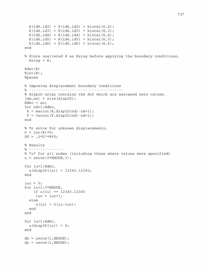
7.17
K(id6,id2) = K(id6,id2) + klocal(6,2); K(id6,id3) = K(id6,id3) + klocal(6,3); K(id6,id4) = K(id6,id4) + klocal(6,4); K(id6,id5) = K(id6,id5) + klocal(6,5); K(id6,id6) = K(id6,id6) + klocal(6,6); end % Store unaltered K as Ksing before applying the boundary conditions. Ksing = K; %det(K) %inv(K); %pause % Imposing displacement boundary conditions % ------------------------------------------ % dispID array contains the dof which are assigned zero values. [sm,sn] = size(dispID); Ndbc = sn; for nd=1:Ndbc, K = matcut(K,dispID(nd)-nd+1); F = veccut(F,dispID(nd)-nd+1); end % To solve for unknown displacements. U = inv(K)*F; SE = .5*U'*K*U; % Results % --------------- % "u" for all nodes (including those where values were specified) u = zeros(3*NNODE,1); for iu=1:Ndbc, u(dispID(iu)) = 12345.12345; end iuc = 0; for iu=1:3*NNODE, if u(iu) == 12345.12345 iuc = iuc+1; else u(iu) = U(iu-iuc); end end for iu=1:Ndbc, u(dispID(iu)) = 0; end dx = zeros(1,NNODE); dy = zeros(1,NNODE);

7.18
for iu=1:NNODE, dx(iu) = u(3*(iu-1)+1); dy(iu) = u(3*(iu-1)+2); end %---------------------------------------------- % Computation of reactions at constrained nodes %---------------------------------------------- R = Ksing*u; Rdisp = zeros(1,Ndbc); for iu=1:Ndbc, Rdisp(iu) = R(dispID(iu)); end %------------------------------------------- % Computation of internal reaction forces % and storing in P(NNODE,4) %------------------------------------------- %M = zeros(NNODE,1); for ie=1:NELEM, eye = ncon(ie,1); jay = ncon(ie,2); % Form the transformation matrix, Lambda. L = Le(ie); A = Ae(ie); lox = (nx(jay)-nx(eye))/L; mox = (ny(jay)-ny(eye))/L; loy = -mox; moy = lox; Lambda = [ lox mox 0 0 0 0 ; ... -mox lox 0 0 0 0 ; ... 0 0 1 0 0 0 ; ... 0 0 0 lox mox 0 ; ... 0 0 0 -mox lox 0 ; ... 0 0 0 0 0 1 ]; % Form local element matrix k(1,1)=E*A/L; k(1,4)=-k(1,1); k(2,2)=12*E*In/(L^3); k(2,3)=6*E*In/(L^2); k(2,5)=-k(2,2); k(2,6)=k(2,3); k(3,2)=k(2,2); k(3,3)=4*E*In/L; k(3,5)=-k(2,3); k(3,6)=2*E*In/L; k(4,1)=-k(1,1); k(4,4)=k(1,1); k(5,2)=-k(2,2); k(5,3)=-k(2,3); k(5,5)=k(2,2); k(5,6)=-k(2,3); k(6,2)=k(2,3); k(6,3)=k(3,6); k(6,5)=-k(2,3); k(6,6)=k(3,3); klocal = Lambda' * k * Lambda;

7.19
% Form ID matrix to identify respective displacements. id1 = 3*(eye-1) + 1; id2 = id1 + 1; id3 = id2 + 1; id4 = 3*(jay-1) +1; id5 = id4 + 1; id6 = id5 + 1; ulocal = [u(id1) u(id2) u(id3) u(id4) u(id5) u(id6)]; Rint = klocal*ulocal'; P(ie,1) = Rint(1); P(ie,2) = Rint(2); P(ie,3) = Rint(3); P(ie,4) = Rint(4); P(ie,5) = Rint(5); P(ie,6) = Rint(6); nxd1 = nx(eye) + u(id1); nyd1 = ny(eye) + u(id2); nxd2 = nx(jay) + u(id4); nyd2 = ny(jay) + u(id5); Ld = sqrt( (nxd2-nxd1)^2 + (nyd2-nyd1)^2 ); if Ld > L P(ie,5) = 1; else P(ie,5) = -1; end if Ld==L P(ie,5) = 0; end end ----------end of fembeam.m----------- ____________________________________

7.20
Exercise 7.3 For the curved beam example, input files are provided below to solve it using the Matlab FEM script.
Verify that the vertical deflection at the point of load application is ⎟⎟⎠
⎞⎜⎜⎝
⎛EIFL3
19213
.
L
L/4
F
Figure 5 A curved beam example
Data files:
____________________________________
node.dat
1 0 0
2 0 1
3 0 2
4 0 3
5 0 4
6 0 5
7 0 6
8 0 7
9 0 8
10 0 9
11 0 10

7.21
12 0 11
13 0 12
14 0 13
15 0 14
16 0 15
17 0 16
18 0 17
19 0 18
20 0 19
21 0 20
22 0.25 20
23 0.5 20
24 0.75 20
25 1.00 20
26 1.25 20
27 0.5 20
28 1.75 20
29 2.00 20
30 2.25 20
31 2.5 20
32 2.75 20
33 3.00 20
34 3.25 20
35 3.5 20
36 3.75 20
37 4.00 20
38 4.25 20
39 4.5 20
40 4.75 20
41 5.00 20
____________________________________
elem.dat
1 1 2 .05 1e7 1.95e-4
2 2 3 .05 1e7 1.95e-4

7.22
3 3 4 .05 1e7 1.95e-4
4 4 5 .05 1e7 1.95e-4
5 5 6 .05 1e7 1.95e-4
6 6 7 .05 1e7 1.95e-4
7 7 8 .05 1e7 1.95e-4
8 8 9 .05 1e7 1.95e-4
9 9 10 .05 1e7 1.95e-4
10 10 11 .05 1e7 1.95e-4
11 11 12 .05 1e7 1.95e-4
12 12 13 .05 1e7 1.95e-4
13 13 14 .05 1e7 1.95e-4
14 14 15 .05 1e7 1.95e-4
15 15 16 .05 1e7 1.95e-4
16 16 17 .05 1e7 1.95e-4
17 17 18 .05 1e7 1.95e-4
18 18 19 .05 1e7 1.95e-4
19 19 20 .05 1e7 1.95e-4
20 20 21 .05 1e7 1.95e-4
21 21 22 .05 1e7 1.95e-4
22 22 23 .05 1e7 1.95e-4
23 23 24 .05 1e7 1.95e-4
24 24 25 .05 1e7 1.95e-4
25 25 26 .05 1e7 1.95e-4
26 26 27 .05 1e7 1.95e-4
27 27 28 .05 1e7 1.95e-4
28 28 29 .05 1e7 1.95e-4
29 29 30 .05 1e7 1.95e-4
30 30 31 .05 1e7 1.95e-4
31 31 32 .05 1e7 1.95e-4
32 32 33 .05 1e7 1.95e-4
33 33 34 .05 1e7 1.95e-4
34 34 35 .05 1e7 1.95e-4
35 35 36 .05 1e7 1.95e-4
36 36 37 .05 1e7 1.95e-4

7.23
37 37 38 .05 1e7 1.95e-4
38 38 39 .05 1e7 1.95e-4
39 39 40 .05 1e7 1.95e-4
40 40 41 .05 1e7 1.95e-4
____________________________________
forces.dat
1 41 2 -2 ____________________________________ disp.dat
1 1 1
2 1 2
3 1 3
____________________________________
Exercise 7.4
The design of a garment hanger is not a big deal. But, it is a good curved-beam problem and plastic
garment hangers do fail occasionally. Using the dimensions shown in Figure 6 and assuming that point A
has a pin-support, Consider the two load cases marked (a) and (b) in the figure. Assume that the hanger is
made out of tubular plastic with 3 mm ID and 7 mm OD. Assume appropriate values for all other data you
need. perform the deflection analysis of the hanger using the Matlab FEM script.

7.24
(a) (b)
-200 -150 -100 -50 0 50 100 150 200
-100
-50
0
50
100
150
200
A
B
C D
E
P
A = (0, 120) B = (-180, 37.59) C = (-180, 0)D = (180, 0) E = (180, 37.59) P = (-173.16, 18.79)
(All dimensions are in mm)
q N/m
q N/m
q N/m
Figure 6 Approximate dimensions for a garment hanger
Exercise 7.5 Modify the Matlab FEM script for beams to compute the stresses. And then use the modified script to estimate stresses in the hanger described in Example 7.2 Exercise 7.6 Derive the shape functions for a higher order beam element that has a mid-side node at 0=ξ in addition
to the nodes at 1−=ξ and 1=ξ . Using those shape functions, construct the element stiffness matrix in the local coordinate system of the beam element.