Beacon Node Placementfor Minimal Localization Error

Zimu Yuan†‡, Wei Li‡, Zhiwei Xu‡, Wei Zhao§†University of Chinese Academy of Sciences, China

‡Institute of Computing Technology, Chinese Academy of Sciences, China§Department of Computer and Information Science, University of Macau, Macau

{yuanzimu, liwei, zxu}@ict.ac.cn, weizhao@umac.mo

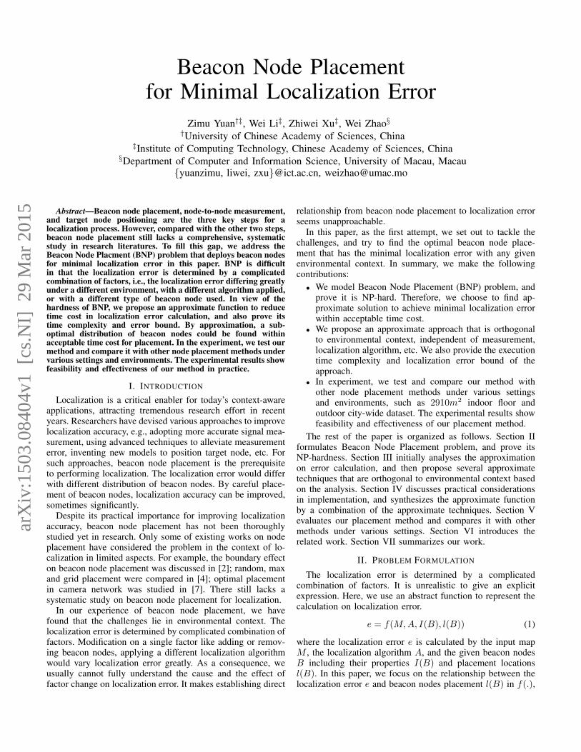
Abstract—Beacon node placement, node-to-node measurement,and target node positioning are the three key steps for alocalization process. However, compared with the other two steps,beacon node placement still lacks a comprehensive, systematicstudy in research literatures. To fill this gap, we address theBeacon Node Placment (BNP) problem that deploys beacon nodesfor minimal localization error in this paper. BNP is difficultin that the localization error is determined by a complicatedcombination of factors, i.e., the localization error differing greatlyunder a different environment, with a different algorithm applied,or with a different type of beacon node used. In view of thehardness of BNP, we propose an approximate function to reducetime cost in localization error calculation, and also prove itstime complexity and error bound. By approximation, a sub-optimal distribution of beacon nodes could be found withinacceptable time cost for placement. In the experiment, we test ourmethod and compare it with other node placement methods undervarious settings and environments. The experimental results showfeasibility and effectiveness of our method in practice.

I. INTRODUCTION

Localization is a critical enabler for today’s context-awareapplications, attracting tremendous research effort in recentyears. Researchers have devised various approaches to improvelocalization accuracy, e.g., adopting more accurate signal mea-surement, using advanced techniques to alleviate measurementerror, inventing new models to position target node, etc. Forsuch approaches, beacon node placement is the prerequisiteto performing localization. The localization error would differwith different distribution of beacon nodes. By careful place-ment of beacon nodes, localization accuracy can be improved,sometimes significantly.

Despite its practical importance for improving localizationaccuracy, beacon node placement has not been thoroughlystudied yet in research. Only some of existing works on nodeplacement have considered the problem in the context of lo-calization in limited aspects. For example, the boundary effecton beacon node placement was discussed in [2]; random, maxand grid placement were compared in [4]; optimal placementin camera network was studied in [7]. There still lacks asystematic study on beacon node placement for localization.

In our experience of beacon node placement, we havefound that the challenges lie in environmental context. Thelocalization error is determined by complicated combination offactors. Modification on a single factor like adding or remov-ing beacon nodes, applying a different localization algorithmwould vary localization error greatly. As a consequence, weusually cannot fully understand the cause and the effect offactor change on localization error. It makes establishing direct

relationship from beacon node placement to localization errorseems unapproachable.

In this paper, as the first attempt, we set out to tackle thechallenges, and try to find the optimal beacon node place-ment that has the minimal localization error with any givenenvironmental context. In summary, we make the followingcontributions:• We model Beacon Node Placement (BNP) problem, and

prove it is NP-hard. Therefore, we choose to find ap-proximate solution to achieve minimal localization errorwithin acceptable time cost.

• We propose an approximate approach that is orthogonalto environmental context, independent of measurement,localization algorithm, etc. We also provide the executiontime complexity and localization error bound of theapproach.

• In experiment, we test and compare our method withother node placement methods under various settingsand environments, such as 2910m2 indoor floor andoutdoor city-wide dataset. The experimental results showfeasibility and effectiveness of our placement method.

The rest of the paper is organized as follows. Section IIformulates Beacon Node Placement problem, and prove itsNP-hardness. Section III initially analyses the approximationon error calculation, and then propose several approximatetechniques that are orthogonal to environmental context basedon the analysis. Section IV discusses practical considerationsin implementation, and synthesizes the approximate functionby a combination of the approximate techniques. Section Vevaluates our placement method and compares it with othermethods under various settings. Section VI introduces therelated work. Section VII summarizes our work.

II. PROBLEM FORMULATION

The localization error is determined by a complicatedcombination of factors. It is unrealistic to give an explicitexpression. Here, we use an abstract function to represent thecalculation on localization error.

e = f(M,A, I(B), l(B)) (1)

where the localization error e is calculated by the input mapM , the localization algorithm A, and the given beacon nodesB including their properties I(B) and placement locationsl(B). In this paper, we focus on the relationship between thelocalization error e and beacon nodes placement l(B) in f(.),

arX

iv:1

503.

0840

4v1

[cs

.NI]

29

Mar

201

5

so as to find a distribution of beacon nodes with the minimallocalization error. We formally define our target as follow.

Problem 1 (Beacon Node Placement (BNP)). Given a map M ,a localization algorithm A, and the information I(B) aboutbeacon nodes, the beacon nodes should be placed on locationsl(B) that minimize the localization error e1.

Theorem 1. BNP is NP-hard.

Proof: (Sketch.) We give an instance of BNP as follows.Let M be a random, bounded area, and A be the trilaterationalgorithm. Assume that the set B of beacon nodes adopts thedistance measurement model, the unit disk coverage model,and the non-sleep energy model. Then, M can be consideredan infinite set IS of location points. Under the specified Aand I(B), the localization error of every location point in IScan be computed independently to determine the localizationerror e.

The above instance can be reduced to the set cover problem[12]. The decision version of the set cover problem is NP-complete, and the optimization version of set cover problemis NP-hard [13]. In the decision version of set cover problem,every element in the universe should be checked if it iscovered by selected subsets. By direct reduction of the errorcomputing function of the above BNP instance to this functionof checking coverage for every (sampled) location point in IS,we can prove that BNP is NP-hard.

III. APPROXIMATE f(.)

A. Basic IdeaIn view of the hardness result for BNP, in this paper we try

to employ an universal approximate approach that can dealwith any map M , any localization algorithm A, and any givenI(B) about beacon nodes. Our approach aims to synthesize afunction f ′(.) instead of f(.) to approximate the calculationof localization error e, so as to find an appropriate solutionwithin acceptable time cost for BNP.

Here, we first discuss the error of approximating f(.). Wedefine the approximate error 4e = |e− e′| = |f(x)− f ′(x′)|,where x = [M, I(B), A, l(B)]. To further analyze the approx-imation error, we introduce 4f ′ and Lf ′ to depict f ′(.). 4f ′

is used to describe the difference between f(.) and f ′(.), andwe have

|f(x)− f ′(x)| ≤ 4f ′ |x| (2)

where |x| denotes a representative value of input. Lf ′ is theLipschitz constant to describe the smoothness of f(.) betweenany two different inputs x and x′, and we have

|f(x)− f(x′)| ≤ Lf |x− x′| (3)

where |x − x′| represents the difference between x and x′.Here, we use an abstract representation of |x| and |x − x′|since their values may be influenced by many hidden factorsthat are hard to infer in an universal approach. And to describethe impact of different factors, we introduce weight vectorW ∈ Rm, having

e = f(x) = f({xj ×Wj | j = 1, 2, ...,m}) (4)

1The localization error e could refer to arithmetic average error, geometricaverage error, median error from a set of results, etc. The techniques discussedlater can be applied no matter which specific meaning it has.

TABLE ISUMMARY OF NOTATIONS

Notation DescriptionM the input map for beacon node placementMs the signal map generated by beacon nodesA the localization algorithm appliedB the set of beacon nodesI(B) the information about beacon nodes including mea-

surement model, energy model, coverage model, etcl(B) the output location for beacon node placementf(.) denoting the function f(M, I(B), A, l(B)) for shorte = f(.) the localization error e for all locations in M can be

calculated by the function f(.)e′ = f ′(.) the approximate error e′ is calculated by the approx-

imate function f ′(.)eopt the minimal localization error can be achieved in the

selected area4e = |e− e′| the absolute difference between e and e′

4f ′ the difference factor between f(.) and f ′(.)Lf ′ the Lipschitz constant for the function f(.)W the weight vector for the inputs of f(.)p a location point in map Mg(.) denoting the relationship between localization error

and distribution of beacon nodesh(.) denoting the signal distribution around a beacon nodeColl the collection of signal points related to a beacon nodeTacc user-specified acceptable calculation time4Eacc user-specified acceptable localization error4Pacc the sampling interval calculated by g(4Eacc)

The function f ′(.) could be composed by a sequence ofapproximate techniques. We use < f ′1(x), f

′2(x), ..., f

′n(x) >

to denote these techniques, and let e′i denote the error changewhen applying f ′i(x) following < f ′1(x), f

′2(x), ..., f

′i−1(x) >.

We have

e′i = f ′i({xj ×Wi,j | i = 1, 2, ..., n, j = 1, 2, ...,m}) (5)

Combine Eq. (2) and Eq. (3), we get

4e = |e−∑n

i=1 e′i|

= |f(x)−∑n

i=1 f′i(x′)|

≤ |f(x)−∑n

i=1 f′i(x)|+

∑ni=1 |f ′i(x)− f ′i(x′)|

≤∑n

i=1

∑mj=1(4f ′

i|xjWi,j |+ Lf ′

i|4xjWi,j |)

(6)

As can be seen from Eq. (6), in general, the approximateerror4e is bounded by the sum of impact of each approximatetechnique and each input factor. For the two powers 4f ′

iand

Lf ′i, if either has a large value, the impact of input factors

would be amplified and thus 4e would become large. Sothe design of approximation should be carefully made tokeep the approximate function f ′(.) smooth and very closeto f(.). However, we should mention the smoothness of f(.)self here. If the applied localization algorithm cannot workstably under various environments (or various input factors),then f(.) self would be unstable, which will make Lf ′

iand

4e have a large value. But we believe it is less likelyto happen when applying those frequently-used localizationalgorithms, otherwise they won’t be adopted in practical use.As for the impact of input factors, stated plainly, the onexi with bigger weight Wi,j would have greater influence.Nevertheless, for our approximate approach, it is impossibleto figure out the exact input factors and their weights which

P9

P1 P2 P3

P4 P5 P6 P7

P8 P10 P11 P12

P13 P14 P15 P16

P17 P18 P19

Fig. 1. A Sampling example. In this example, location point p1, p2, ...,p19 are uniformly sampled in the hexagon; 3 beacon nodes are planed to beplaced in this hexagon. By sampling, there are altogether C3

19 combinationsfor beacon node placement; for each combination, the worker measures thesignal in these 19 points. In the figure, 3 beacon node are placed on p5, p11and p14 respectively, and the worker is at p9.

depend on the specific localization scene. For this reason, weshall consider every location point in M as equally importantin approximation so as to avoid deviation on input factors.Later we will show how to design techniques on approximationaccording to this discussion.

B. Techniques on ApproximationWe propose several techniques on approximating f(.) in

this section. These include Sampling, Memorization, Skippingand Interpolation. All of these techniques are proposed forreducing the execution time cost for BNP, and can be appliedindividually.

1) Sampling: For some localization scenes, it is impossibleto calculate out the error on every location point in M withinan accepted time cost. A natural way is to efficiently sampleuseful location points in M to approximate the localizationerror e. As discussed, we are not able to infer the exact inputfactors and their weights in the universal approach. So weapply uniform sampling on M to treat every location pointas equally important. The approximate function f ′(.) with thesampling technique applied would have a reduced calculationtime compared to directly calculate e by the function f(.).We illustrate a sampling example in Fig. 1. In this example,a hexagon on the map is sampled with uniformly distributedlocation points.

2) Memorization: Usually, the coverage range of a beaconnode is limited. Therefore, we can memorize the calculationresults of a selected area to infer the results of other areas.More specifically, when calculating the localization error witha given distribution of beacon nodes, we can look up the mem-orized results for the same or similar beacon node distributionas an approximation to reduce the calculation time. As shownin Fig. 2, 3 beacon nodes are located at point p1, p2, and p3separately inside a hexagon. If the memorized results of thehexagon (with dashed line) have 3 beacon nodes with theirdistribution |p′i − p1|+ |p′j − p2|+ |p′k − p3| ≤ Tmem, whereTmem is a threshold distance value set up, then the error ofdistribution p1, p2 and p3 can be approximated by the resulton the distribution pi, pj and pk.

3) Skipping: A bad distribution of beacon nodes would notbe a good approximation of f(.), and thus can be ignored inerror calculation to reduce the time cost. Intuitively, we caninfer a distribution to be a bad one based on previous results.As discussed in Section III-A, we assume that frequently-used localization algorithms are stable ones, otherwise theywould not be used in a practical manner. Therefore, for a

P1

P2

P3

Pi

Pj

Pk

Pk ′

Pi ′

Pj ′

Fig. 2. A Memorization example. Suppose that the calculation results ofbeacon node placement in the hexagon with dashed line have already beenmemorized. When deploying beacon nodes in the hexagon with solid line,similar node distributions can be looked up for in the memorized results. Inthe figure, we translate pi, pj , pk to p′i, p

′j , p′k by the vector pi~p1 respectively.

If |p′i−p1|+|p′j−p2|+|p′k−p3| ≤ Tmem, we consider that the distributionof p1, p2 and p3 could be approximated by pi, pj and pk .

P9

P2

P3

P4 P5

P6 P7 P8

P10 P11P12 P13

P14 P15

P1

Fig. 3. A Skipping example. Suppose that some distributions of beaconnodes are shown as bad ones during previous calculation. Then, when beaconnodes are deployed with the distribution similar to bad ones, we can inferthat these nodes are also in a bad arrangement. In the figure, the set of pointsnearest in different directions are found for p1, p2 and p3 respectively. Forany combination of pi ∈ {p4, p5, p6, p7}, pj ∈ {p8, p9, p10, p11} andpk ∈ {p12, p13, p14, p15}, if |pi − p1| + |pj − p2| + |pk − p3| ≤ Tskpand the combination of pi, pj and pk has unacceptable localization error, weconsider that the calculation on p1, p2, and p3 can be skipped.

specific distribution of beacon nodes, if all its similar distri-butions have unbefitting error, we believe that this distributioncould be skipped without calculation. We also set a distancethreshold value Tskp for Skipping. Generally speaking, wehave Tskp > Tmem since the result for reuse should be moreaccurate than the result for inferring its bad or good. TakeFig. 3 for example. For any distribution pi ∈ {p4, p5, p6, p7},pj ∈ {p8, p9, p10, p11}, pk ∈ {p12, p13, p14, p15}, if we have|pi − p1| + |pj − p2| + |pk − p3| ≤ Tskp and the distributionof pi, pj , and pk is considered as an unaccepted one forapproximation, we choose to skip the error calculation on thedistribution of p1, p2, and p3.

4) Interpolation: The function f(.) self could be involvedwith complex error calculation. Either f(.) has a non-linear,complex form which may take a lot of time on calculation,or it cannot be directly derived in theory which needs anumerical simulation approach. To deal with the case, weuse polynomials to approximate f(.) based on its form orits numerical simulation results. For example, ex can beapproximated by its Taylor series

∑ci=0 x

i/i!, if ∃c having|∑c

i=0 xi/i!− ex| ≤ 4ε where 4ε is a defined limited error

on approximation.

Algorithm 1: ErrorOnDistributionInput: Input map M , the localization algorithm A, the

set of beacon nodes B, information I(B) aboutbeacon nodes

Output: The relationship g(.) between localization errorand distribution of beacon nodes

1 for j = 1, 2, ...n do2 Randomly assign locations pi, i = 1, 2, ..., |B|, to

beacon nodes B;3 Randomly generate an offset distance 4pi;4 Randomly move beacon node with∑|B|

i=1 |p′i − pi|/|B| = 4pi;5 Calculate the difference error 4e between

{pi, i = 1, 2, ..., |B|} and {p′i, i = 1, 2, ..., |B|};6 Store (4pi,4ei);7 end8 Fit 4p = g(4e) by {(4pi,4ei)|i = 1, 2, ..., n};9 return g(.);

Algorithm 2: SelectedAreaInput: Acceptable calculation time Tacc and localization

error 4Eacc, the relationship g(.) betweenlocalization error and distribution of beaconnodes, input map M , the localization algorithmA, the set of beacon nodes B, information I(B)about beacon nodes

Output: The selected area Area1 Calculate the offset distance 4Pacc = g(4Eacc);2 Set the sampling density ds = 1/4P 2

acc point/size;3 Set the beacon node density db = |B|/|M | node/size;4 Time the execution of f ′(.) as t;5 Solve the area size S by max(S) s.t. CS·db

S·ds· t ≤ Tacc;

6 Select an area Area (such as a regular hexagon) of sizeS;

7 return Area;

IV. THE PROPOSED BNP ALGORITHM

A. Practical ConsiderationWith the NP-hardness of BNP, it is infeasible to directly

calculate on f(.) for optimal beacon node placement. In-stead, we apply the techniques discussed in Section III-B toapproximate f(.). Nevertheless, to combine these techniquesin the system, three critical issues should be considered forus in implementation. The first is to let the approximatefunction f ′(.) execute within acceptable time. The second isto characterize localization environment on the execution off ′(.). The third is to consider the boundary of map for BNP.Next we address these three issues respectively.

1) Strategy on Error-Time Trade-off: As discussed in Sec-tion III-B2, the distributed pattern of beacon nodes in a se-lected area can be memorized to infer beacon node placementin other areas. At the same time, when applying memorization,a trade-off in area size inevitably occurs: either to explore alarger area for memorization to provide more accurate approx-imation of f(.), or a smaller area to reduce the calculationtime of f ′(.). To deal with this trade-off, we should select an

Algorithm 3: ModelingNodeInput: Input map M , the set of beacon nodes B,

information I(B) about beacon nodesOutput: the collection Coll of signal points, the fitting

expression h(.) of signal related to a beaconnode

1 User places a beacon node b on a point p in M ;2 Gather the signal points around b to the collection Coll;3 Fit the relation of signal points to b as the expressionh(.);

4 return Coll and h(.);

Algorithm 4: ModelingAreaInput: Input map M , the set of beacon nodes B,

information I(B) about beacon nodes, thecollection Coll of signal points, the fittingexpression h(.) of signal related to a beacon node

Output: The signal map Ms

1 for Each signal point p in M do2 if Similar points found in Coll then3 Generate signal by the expected value of similar

points;4 else5 Generate signal by h(.);6 end7 Record the generated signal to Ms;8 end9 return Ms;

area of proper size to balance between localization error andcalculation time.

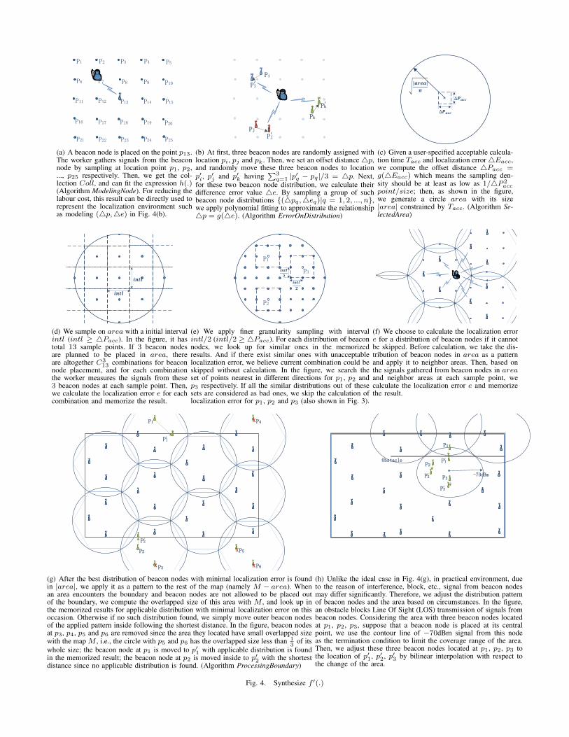
To select a proper sized area, we first try to determinethe relationship between localization error and distribution ofbeacon nodes by random assignment. As illustrated in Fig.4(b), three beacon nodes are randomly assigned with locationpi, pj and pk. We set an offset distance 4p, and randomlymove the beacon nodes to location p′i, p

′j and p′k having∑3

q=1 |p′q − pq|/3 = 4p. Then, for these two beacon nodedistributions, we calculate their difference value, 4e, on error.By sampling a group of such beacon node distributions, wehave {(4pq,4eq)|q = 1, 2, ..., n}. We use polynomial fittingto approximate the relationship between 4p and 4e, formallyas 4p = g(4e). We summarize the process in Algorithm 1— ErrorOnDistribution.

Based on g(.), Algorithm 2 – SelectedArea – gives a sketchon determining the size of selected area for memorization.SelectedArea takes the acceptable calculation time Tacc andacceptable localization error4Eacc as the user-specified input.Within the limit of Tacc, the approximate function f ′(.) has|f ′(.) − f(.)| ≤ 4Eacc. In process, SelectedArea uses thesampling density ds and the beacon node density db to estimatethe area size S by max(S), s.t. CS·db

S·ds· t ≤ Tacc, that is, to

select an area of proper size by considering both Tacc and4Eacc with respect to the execution time of f ′(.).

In addition, we use α · CS·db

S·ds· t ≤ 4Eacc with an

approximate ratio 0 < α < 1 in practical calculation, since

techniques on approximation are applied, i.e., some executionof f ′(.) are skipped (Section III-B3). We omit the detail aboutα due to it is not a primary concern in our paper.

2) Strategy on Characterization of Localization Environ-ment: Naturally, we can place beacon nodes in differentdistributions to characterize the environment, and thus to finda relatively lower localization error e′. However, it wouldcost abundant labor in placement with repeatedly adjustingthe position of beacon nodes and calculating their localizationerror distributions. Also, freely moving beacon nodes areimpossible in some localization scenes, i.e., beacon nodes needelectric plug. So we believe it is not an applicable way for ourgeneral approach of BNP.

Instead, we apply a modeling approach based on mea-surement results. First, we gather the strength (or sometimesthe direction) of signal points scattered over an area or astraight line from a beacon node as a collection Coll, andapply Interpolation (Section III-B4) to fit the expression h(.)of signal strength (or direction) related to a beacon node.We summarize these course of actions in Algorithm 3 –ModelingNode. Then, when modeling the whole map, forevery point, we search in the collection Coll for similar ones,and generate signal by the expected value of these similarones; otherwise, if no similar point found, we generate a signalby the fitting expression h(.). Algorithm 4 – ModelingArea –depicts the process of modeling beacon node placement. Laterin the experiment (Section V), we also describe the processof ModelingArea in practical environment.

3) Strategy on The Boundary of Map: In practical deploy-ment, the input map M should be considered with boundary.When there is an existing boundary, we need to addresstwo cases in BNP separately. In one, beacon nodes may beplaced outside of the boundary. Therein, BNP can be regardedas working on the unbounded area, and we only need toplace beacon nodes to cover M . The other is that beaconnodes cannot be placed out of the boundary, i.e., beaconnodes cannot be placed outside in the second floor of abuilding. In this case, we search in the memorized resultsfor the beacon node distribution with two criteria: all beaconnodes are located inside the boundary; the localization errorshould be minimized on this occasion. Otherwise if no suchdistribution is found, we search for the best memorized resultwith minimal localization error, and move each outer beaconnode of this result inside following the shortest distance. Thisprocess on the boundary of map is also described in Algorithm5 – ProcessingBoundary.

B. The Algorithm and Complexity

Combining all the discussions above, we can synthesizethe approximate function f ′(.) and find a sub-optimal beaconnode placement by Algorithm 6. The main idea behind it is todivide-and-conquer the calculation of f(.) on M , by which wecan lower down the calculation time to a user-specified Tacc;place beacon nodes to locations l(B) with the localizationerror kept at most 4Eacc (or γ4Eacc addressed later) greaterthan the error by the optimal beacon node placement.

To clearly understand the process of synthesization in Al-gorithm 6, we explain it with demonstrations in Fig. 4. Inline 1, we collect signals from a beacon node at scatteredlocation points as collection coll and fit the expression h(.)

Algorithm 5: ProcessingBoundaryInput: Input map M , the set of beacon nodes B,

information I(B) about beacon nodes, memorizedresult memo, the output location l(B)

Output: The output location l(B)1 Let dbest be the distribution with minimal localization

error in memo;2 if Beacon nodes are allowed to be placed outside M

then3 Write l(B) according to dbest;4 else5 Look up memo for the distribution d with beacon

nodes inside the boundary and minimal localizationerror;

6 if d 6= Null then7 Write l(B) according to d;8 else9 Write l(B) by moving each outer beacon node of

dbest inside following the shortest distance;10 end11 end12 return l(B);

by Algorithm ModelingNode (Fig. 4(a)). In line 2, we modelthe relationship g(.) between the offset distance 4p and thedifference error 4e by Algorithm ErrorOnDistribution (Fig.4(b)). In line 3, taking user-specified acceptable calculationtime Tacc and localization error 4Eacc as input, we selecta circle area with its size constrained by Tacc and 4Eacc

in Algorithm SelectedArea (Fig. 4(c)). In line 4-32, we applysampling on area. At the beginning of sampling process, wefirstly compute the acceptable sampling interval 4Pacc, andselect a initial interval intl (intl ≥ 4Pacc) (Fig. 4(d)). Then,during sampling process, we examine each combination ofbeacon node distribution (line 12-26). For a distribution, if allthe similar distributions are considered to be bad ones, we skipits calculation (Fig. 4(e)); else we calculate the localizationerror on this distribution and memorize the result (Fig. 4(f)).Besides, in line 27-39, we use polynomials to approximatethe error calculation after obtaining a set of results. Next, inline 33-41, we apply the best distribution found in area as apattern to the rest of map M − area. In it, we consider twoproblems in practical deployment. The first is to deal withthe boundary of map M . When a beacon node is not allowedto be placed out of the boundary, we either move this nodeinside or just remove it (Fig. 4(g)). The other is to adjust thedistribution pattern of beacon nodes and the area based onpractical environment (Fig. 4(h)).

In brief, the synthesization process looks up for the bestdistribution in a selected area, and applies it as a patternto the rest of the map. A hypothesis behind it is that theerror distribution of the selected area is the same as otherareas in the map. Thus, we define an ideal case: the errordistribution in each circle (or regular hexagon) is the same(namely the function g(.) can be applied globally); beaconnodes can be placed out of the boundary. Let eopt denote theminimal localization error can be achieved in the selected area.We have Theorem 2 on time complexity and localization error

P9

P1 P2 P3 P4 P5

P6 P7 P8 P10

P11 P12 P13 P14 P15

P16 P17 P18 P19 P20

P21 P22 P23 P24 P25

(a) A beacon node is placed on the point p13.The worker gathers signals from the beaconnode by sampling at location point p1, p2,..., p25 respectively. Then, we get the col-lection Coll, and can fit the expression h(.)(Algorithm ModelingNode). For reducing thelabour cost, this result can be directly used torepresent the localization environment suchas modeling (4p,4e) in Fig. 4(b).

Pi

Pj

Pk

Pk ′

Pi ′

Pj ′

(b) At first, three beacon nodes are randomly assigned withlocation pi, pj and pk . Then, we set an offset distance4p,and randomly move these three beacon nodes to locationp′i, p′j and p′k having

∑3q=1 |p′q − pq |/3 = 4p. Next,

for these two beacon node distribution, we calculate theirdifference error value 4e. By sampling a group of suchbeacon node distributions {(4pq ,4eq)|q = 1, 2, ..., n},we apply polynomial fitting to approximate the relationship4p = g(4e). (Algorithm ErrorOnDistribution)

(c) Given a user-specified acceptable calcula-tion time Tacc and localization error4Eacc,we compute the offset distance 4Pacc =g(4Eacc) which means the sampling den-sity should be at least as low as 1/4P 2

accpoint/size; then, as shown in the figure,we generate a circle area with its size|area| constrained by Tacc. (Algorithm Se-lectedArea)

(d) We sample on area with a initial intervalintl (intl ≥ 4Pacc). In the figure, it hastotal 13 sample points. If 3 beacon nodesare planned to be placed in area, thereare altogether C3

13 combinations for beaconnode placement, and for each combinationthe worker measures the signals from these3 beacon nodes at each sample point. Then,we calculate the localization error e for eachcombination and memorize the result.

P1

P2

P3

(e) We apply finer granularity sampling with intervalintl/2 (intl/2 ≥ 4Pacc). For each distribution of beaconnodes, we look up for similar ones in the memorizedresults. And if there exist similar ones with unacceptablelocalization error, we believe current combination could beskipped without calculation. In the figure, we search theset of points nearest in different directions for p1, p2 andp3 respectively. If all the similar distributions out of thesesets are considered as bad ones, we skip the calculation oflocalization error for p1, p2 and p3 (also shown in Fig. 3).

(f) We choose to calculate the localization errore for a distribution of beacon nodes if it cannotbe skipped. Before calculation, we take the dis-tribution of beacon nodes in area as a patternand apply it to neighbor areas. Then, based onthe signals gathered from beacon nodes in areaand neighbor areas at each sample point, wecalculate the localization error e and memorizethe result.

P1

P1 ′

x

x

xx

P2

P2 ′

P3

P4

P5

P6

(g) After the best distribution of beacon nodes with minimal localization error is foundin |area|, we apply it as a pattern to the rest of the map (namely M − area). Whenan area encounters the boundary and beacon nodes are not allowed to be placed outof the boundary, we compute the overlapped size of this area with M , and look up inthe memorized results for applicable distribution with minimal localization error on thisoccasion. Otherwise if no such distribution found, we simply move outer beacon nodesof the applied pattern inside following the shortest distance. In the figure, beacon nodesat p3, p4, p5 and p6 are removed since the area they located have small overlapped sizewith the map M , i.e., the circle with p5 and p6 has the overlapped size less than 1

3of its

whole size; the beacon node at p1 is moved to p′1 with applicable distribution is foundin the memorized result; the beacon node at p2 is moved inside to p′2 with the shortestdistance since no applicable distribution is found. (Algorithm ProcessingBoundary)

-70dBm

P1

P1 ′

P2

P2 ′ P3

P3 ′

Obstacle

(h) Unlike the ideal case in Fig. 4(g), in practical environment, dueto the reason of interference, block, etc., signal from beacon nodesmay differ significantly. Therefore, we adjust the distribution patternof beacon nodes and the area based on circumstances. In the figure,an obstacle blocks Line Of Sight (LOS) transmission of signals frombeacon nodes. Considering the area with three beacon nodes locatedat p1, p2, p3, suppose that a beacon node is placed at its centralpoint, we use the contour line of −70dBm signal from this nodeas the termination condition to limit the coverage range of the area.Then, we adjust these three beacon nodes located at p1, p2, p3 tothe location of p′1, p′2, p′3 by bilinear interpolation with respect tothe change of the area.

Fig. 4. Synthesize f ′(.)

for the synthesization process.

Theorem 2. In the ideal case, the synthesization process(Algorithm 6) executes with time complexity of O(Tacc) andgenerates the distribution of beacon nodes with localizationerror e− eopt ≤ γ4Eacc, γ ≥ 0.

Proof: In the selected area, we have the total calculationtime CS·db

S·ds· t ≤ Tacc (Line 5, Algorithm SelectedArea). The

best distribution found in the selected area can be directlyapplied to other areas. Therefore, the synthesization processhas time complexity O(Tacc).

Let Popt be the best distribution of beacon nodes found,having the minimal localization error eopt. With the samplinginterval set to 4Pacc (Line 1, Algorithm SelectedArea), wecan find a distribution P with localization error e, having|P − Popt| ≤

√22 Pacc. It has the error e ≥ eopt if the

approximate function f ′(.) does not change the monotonicityof f(.). As can be seen, the approximate techniques (Sampling,Memorization, Skipping, and Interpolation) applied in the syn-thesization process do not change the original monotonicity oferror distribution. (For Interpolation, if it has low error.) Thus,we can infer that the approximate function f ′(.) is monotoneincreasing around Popt. (Namely, |P−Popt| ∝ e−eopt.) Recallthat 4Pacc = g(4Eacc). For |P − Popt| ≤

√22 Pacc, we have

e− eopt ≤ γ4Eacc, γ ≥ 0.In a practical environment, it is complicated to determine

γ in Theorem 2 since the value of γ depends on the givenmap, localization algorithm, and the information about beaconnodes. As discussed in Section III, the frequently-used local-ization algorithms are less likely to be unstable in smoothness,otherwise they would not be used in practical. Thus, we believethat drastic variations on error distribution are unlikely tohappen, and γ usually has a small value.

V. EXPERIMENTAL ANALYSIS

In this section, we evaluate our beacon node placementmethod in actual environments. First, we change the size of theselected area and the sampling interval to assess our methodon execution time and localization error. Then, we compareour method with several other placement methods in indoorenvironment. Finally, we also experiment on a large scale,outdoor real-world dataset.

A. Experiment Setting

The experiment setting is as follows.Measurement and Localization Algorithm: There exist nu-

merous studies on measurement and algorithm for localization.Among these studies, WiFi based localization has attractedtremendous attention for its wide availability and no extradeployment cost in recent years. Most of existing WiFi basedlocalization algorithms can be divided into two categories:Model-based and Fingerprinting-based. In our experiment, weconsider WiFi measurement and select EZPerfect [5][17] andRADAR [3], which are representative of model-based andfingerprinting-based algorithm respectively.• EZPerfect trains the parameters of the log-distance path

loss model by sampling signals at selected locations,and apply Trilateration or Multilateration to estimate thelocation of target points.

Algorithm 6: Beacon Node PlacementInput: Input map M , the localization algorithm A, the

set of beacon nodes B, information I(B) aboutbeacon nodes, user-specified acceptablecalculation time Tacc and localization error 4Eacc

Output: The output location l(B) of beacon nodes1 [coll, h(.)] =ModelingNode(M,B, I(B));2 g(.) = ErrorOnDistribution(M,A,B, I(B));3 area =SelectedArea(M,A,B, I(B), g(.), Tacc,4Eacc);

4 n = |area| · |B|/|M |; //Number of nodes to be placed5 4Pacc = g(4Eacc); //Acceptable sampling interval6 User set the interval intl (intl ≥ 4Pacc);7 Set the error e =∞;8 Set the location l(B) = 0;9 while intl ≥ 4Pacc do

10 //Apply Sampling11 m = |area|/intl2; //Number of points to be sampled12 foreach Beacon node distribution {pi|i = 1, 2, ..., n}

out of all Cnm combinations do

13 ModelingArea(M,B, I(B), Coll, h(.));14 //Apply Skipping15 if {pi|i = 1, 2, ..., n} can be skipped then16 Continue;17 else18 Calculate the localization error e′ by

sampling (namely using f ′(.));19 if e′ < e then20 e = e′;21 Record the locations of beacon nodes to

l(B);22 end23 //Apply Memorization24 Memorize {pi|i = 1, 2, ..., n} and e′ to

memo;25 end26 end27 //Apply Interpolation28 if the error calculation can be interpolated then29 Use polynomials to approximate the error

calculation (namely approximate f ′(.));30 end31 intl = intl/2;32 end33 Split the remaining area M − area to{areai | i = 1, 2, ..., q};

34 Let dbest be the distribution with minimal localizationerror in memo;

35 foreach areai in {areai | i = 1, 2, ..., q} do36 if areai contains boundary then37 l(B) =

ProcessingBoundary(M,B, I(B), l(B),memo);38 else39 Write l(B) according to dbest;40 end41 end42 return l(B);

向下

向上

45 m

96 m

25 m

35 m

拖动侧边手柄更

改文本块的宽

度。

3437.17

Fig. 5. At the beginning of the experiments, we randomly deploy some China Mobile M601 phones, with WiFi hotspot turned on, as beacon nodes. Thenwe use an AmigoBot with a phone placed on it traveling around the floor to gather signals from these beacon nodes.

TABLE IITHE EXECUTION TIME OF OUR PLACEMENT METHOD (ALGORITHM 6) ON

EZPEFECT IN INDOOR ENVIRONMENT

EZPerfect 1m 2m 3m 4m 5mS 5.36 ×

1051(e.)5.27 ×1039(e.)

4.34 ×1032(e.)

3.57 ×1027(e.)

2.84 ×1024(e.)

14S 1.62 ×

1011(e.)1.52 ×108(e.)

2.52 ×106(e.)

2.21 ×105(e.)

1.78 ×104(e.)

19S 1.01 ×

105(e.)1631.23 125.96 25.18 12.08

116

S 1.09 ×104(e.)

257.35 15.07 8.15 0.75

125

S 3.02 ×103(e.)

45.14 6.14 0.56 0.25

1 All values are in seconds, or s. The estimated values are with thesuffix ’(e.)’. The selected area size and sampling interval vary fromS to 1

25S, and 1m to 5m respectively.

• RADAR collects fingerprints of signals at known locationsto establish a fingerprint database, and then determinesthe location of a target point by averaging the locationsof these nearest fingerprints found in the database.

Beacon Node Placement Method: For comparison, we im-plement four other placement methods, including two randomones and two deterministic ones.• Random optionally selects location points for beacon

node placement. In the experiment, we generate distri-bution of beacon nodes for 3 times, and show the bestresult among them.

• RKC [11] assigns beacon nodes to location points thatare randomly selected from the near-optimal hitting setsfor k-covering area. We also generate beacon node distri-bution for 3 times and show the best result among them.

• Uniform places beacon nodes at regular intervals.• CERACC [1] deterministically assigns beacon nodes to

the lenses of slices in triangle lattice pattern for k-covering area.

Localization Error: We use the following four error repre-sentations as the metric to evaluate the quality of beacon nodeplacement method.• Arithmetic mean error (ari.): eari. = 1

n

∑ni=1 ei

• Geometric mean error (geo.): egeo. = n√∏n

i=1 ei• Median error (med.): Let e1 ≤ e2 ≤ ... ≤ en. If n%2 ==

0, then emed. = en+12

; otherwise emed. = (en2+en

2 +1)/2.

TABLE IIITHE EXECUTION TIME OF OUR PLACEMENT METHOD (ALGORITHM 6) ON

RADAR IN INDOOR ENVIRONMENT

RADAR 1m 2m 3m 4m 5mS 4.65 ×

1051(e.)4.30 ×1039(e.)

3.49 ×1032(e.)

8.20 ×1027(e.)

2.75 ×1024(e.)

14S 1.15 ×

1011(e.)1.16 ×108(e.)

1.79 ×106(e.)

1.73 ×105(e.)

1.33 ×104(e.)

19S 7.45 ×

104(e.)1229.61 97.44 21.77 9.38

116

S 8.37 ×103(e.)

203.07 13.08 6.01 0.54

125

S 2.35 ×103(e.)

34.94 4.92 0.41 0.19

• Proportion of abnormal errors (abn.): Let bi = 1 if ei ≥2eari., else set bi = 0. Then pabn. =

∑ni=1 bin × 100%.

Experimental Environment: We experiment in two localiza-tion environments, with their difference on the type of beaconnode, signal transmission, and scale.

• Indoor Environment: We conduct the indoor experimentsin the floor, shown in Fig. 5, with its area size S =2910m2. In experiments, we use a total of 20 mobilephones as beacon nodes to create WiFi hotspots. At thebeginning of the experiments, we control an AmigoBotwith a mobile phone walking around the floor, gatheringsignals at location points. Then, we divide the gatheredsignals into several collections coll1, coll2, ..., colln bydistinguishing number of walls from the WiFi hotspot tothe location point receiving signal, and fit the expressionh1(.), h2(.), ..., hn(.) (Algorithm ModelingNode).

• Outdoor Environment: We directly use the MetroFidataset [22]. It involves 72 access points and samplessignals at over 200, 000 location points in a city-widearea. These location points are taken as candidate loca-tions for beacon node placement, and the access pointsare considered as the target nodes for localization inexperiments. We take the whole dataset as collection coll,and fit the expression h(.).

All the placement methods and localization algorithms wereimplemented with VC++. All the calculation were running ona Windows 7 machine with 2.3GHZ Intel Core i7 CPU and8GB RAM.

TABLE IVTHE LOCALIZATION ERROR OF OUR PLACEMENT METHOD (ALGORITHM 6) ON EZPEFECT IN INDOOR ENVIRONMENT

EZPerfect 2m 3m 4m 5mari. geo. med. abn. ari. geo. med. abn. ari. geo. med. abn. ari. geo. med. abn.

19S 2.85 2.28 2.47 6.82% 3.05 2.45 2.59 6.58% 3.12 2.48 2.68 7.06% 3.95 3.15 2.97 7.40%

116

S 2.94 2.33 2.57 7.08% 3.88 3.01 3.03 8.82% 4.05 3.24 3.09 9.09% 4.21 3.31 3.26 10.04%125

S 3.10 2.51 2.68 8.81% 4.11 3.41 3.08 9.28% 4.29 3.49 3.80 11.78% 4.50 3.66 3.89 12.52%1 All values of error are in meters or m, except abn. using percentage.

TABLE VTHE LOCALIZATION ERROR OF OUR PLACEMENT METHOD (ALGORITHM 6) ON RADAR IN INDOOR ENVIRONMENT

RADAR 2m 3m 4m 5mari. geo. med. abn. ari. geo. med. abn. ari. geo. med. abn. ari. geo. med. abn.

19S 3.09 2.31 3.01 0% 3.18 2.58 2.82 0% 3.23 2.72 2.90 0% 3.50 3.06 2.77 4.92%

116

S 3.13 2.70 3.27 3.70% 3.49 2.96 2.94 1.72% 3.51 3.05 3.45 4.01% 3.55 3.14 3.18 5.62%125

S 3.19 2.76 3.05 0% 3.53 3.03 3.29 4.12% 3.82 3.12 3.56 4.76% 4.09 3.25 3.79 7.41%

向下

向上

(a) Random

向下

向上

(b) RKC

向下

向上

(c) Uniform

向下

向上

(d) CERACC

Fig. 6. Beacon Node Placement

B. The Impact of Selected Area Size and Sampling Intervalon Execution time

Here, we introduce the experimental results of our beaconnodes placement methods on execution time in an indoorenvironment. In experiments, we vary the size of selectedarea from S to 1

25S, and sampling interval from 1m to 5m,timing the execution of our placement method on localizationalgorithm EZPerfect and RADAR. The results of executiontime on EZPerfect and RADAR are shown in Table II and IIIrespectively (with some non-computable items estimated byCS·db

S·ds· t in Algorithm SelectedArea). As can be seen from

the results, by applying techniques (Sampling, Memorization,Skipping, and Intepolation) on approximation, we can largelyreduce the execution time on finding beacon node distributionfor placement, i.e., the execution time of our placementmethod with selected area size 1

9S and sampling interval 2m( 19S, 2m) on EZPerfect reduced by a factor of 3.29 × 1048

compared to the case of (S, 1m). This experimental resultshows the effectiveness of the approximate techniques applied.Besides, we do not verify the effectiveness of each techniqueindependently here since it is not the major concern in ourevaluation.

C. The Impact of Selected Area Size and Sampling Intervalon Localization Error

Next, we focus on the impact of varying the size of aselected area and sampling interval on localization error. In

TABLE VITHE LOCALIZATION ERROR OF THE REFERENCED METHODS ON

EZPERFECT IN INDOOR ENVIRONMENT

EZPerfect ari. geo. med. abn.Random 6.26 5.16 5.25 15.09%

RKC 4.42 3.56 3.77 8.08%Uniform 4.66 3.77 3.86 6.56%

CERACC 5.91 4.63 4.12 8.06%

TABLE VIITHE LOCALIZATION ERROR OF THE REFERENCED METHODS ON RADAR

IN INDOOR ENVIRONMENT

RADAR ari. geo. med. abn.Random 5.52 4.41 4.89 12.32%

RKC 4.14 3.29 3.74 9.57%Uniform 4.11 3.28 3.81 7.60%

CERACC 4.95 4.21 4.01 8.58%

the experiment, we target finding the beacon node distributionwith minimal arithmetic mean error. (Besides, we can getsimilar results using other error representations. Due to spacelimits, we omit them here.) The results on EZPerfect andRADAR are shown in Table IV and V respectively. As canbe seen from both of these two table, 1) the localizationerror increases as the selected area size changes from 1

9Sto 1

25S; 2) the localization error increases as the samplinginterval changes from 2m to 5m. The reason for the errorincrease is that the search space for beacon node placement ispruned when increasing the sampling interval, or decreasingthe selected area size. As discussed in Section IV-B, wecan take user-specified acceptable calculation time Tacc andlocalization error 4Eacc as input to select a proper samplinginterval and area. I.e., specifying Tacc = 1632.23s, andeopt +4Eacc ≤ 2.85, we can select an area with size being13S and interval being 2m for sampling.

D. Comparison in Indoor EnvironmentWe apply four other placement methods, two random ones

(Random and RKC) and two deterministic ones (Uniform andCERACC), as reference for comparison. The beacon nodesplaced by these methods are shown in the sub-figures of Fig.6 separately. The corresponding localization errors of thesemethods on EZPerfect and RADAR are shown in Table VI andVII respectively. As can be seen from both of these two tables,

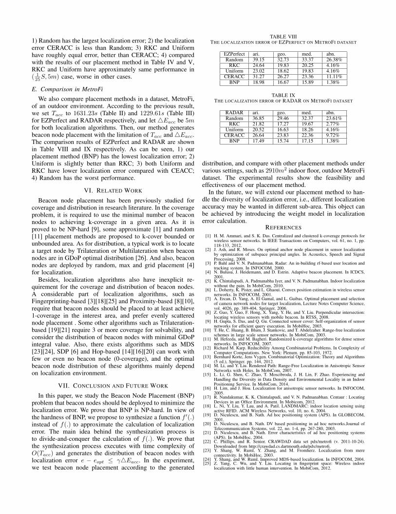
1) Random has the largest localization error; 2) the localizationerror CERACC is less than Random; 3) RKC and Uniformhave roughly equal error, better than CERACC; 4) comparedwith the results of our placement method in Table IV and V,RKC and Uniform have approximately same performance in( 125S, 5m) case, worse in other cases.

E. Comparison in MetroFi

We also compare placement methods in a dataset, MetroFi,of an outdoor environment. According to the previous result,we set Tacc to 1631.23s (Table II) and 1229.61s (Table III)for EZPerfect and RADAR respectively, and let 4Eacc be 5mfor both localization algorithms. Then, our method generatesbeacon node placement with the limitation of Tacc and4Eacc.The comparison results of EZPerfect and RADAR are shownin Table VIII and IX respectively. As can be seen, 1) ourplacement method (BNP) has the lowest localization error; 2)Uniform is slightly better than RKC; 3) both Uniform andRKC have lower localization error compared with CEACC;4) Random has the worst performance.

VI. RELATED WORK

Beacon node placement has been previously studied forcoverage and distribution in research literature. In the coverageproblem, it is required to use the minimal number of beaconnodes to achieving k-coverage in a given area. As it isproved to be NP-hard [9], some approximate [1] and random[11] placement methods are proposed to k-cover bounded orunbounded area. As for distribution, a typical work is to locatea target node by Trilateration or Multilateration when beaconnodes are in GDoP optimal distribution [26]. And also, beaconnodes are deployed by random, max and grid placement [4]for localization.

Besides, localization algorithms also have inexplicit re-quirement for the coverage and distribution of beacon nodes.A considerable part of localization algorithms, such asFingerprinting-based [3][18][25] and Proximity-based [8][10],require that beacon nodes should be placed to at least achieve1-coverage in the interest area, and prefer evenly scatterednode placement . Some other algorithms such as Trilateration-based [19][21] require 3 or more coverage for solvability, andconsider the distribution of beacon nodes with minimal GDoPintegral value. Also, there exists algorithms such as MDS[23][24], SDP [6] and Hop-based [14][16][20] can work withfew or even no beacon node (0-coverage), and the optimalbeacon node distribution of these algorithms mainly dependon localization environment.

VII. CONCLUSION AND FUTURE WORK

In this paper, we study the Beacon Node Placement (BNP)problem that beacon nodes should be deployed to minimize thelocalization error. We prove that BNP is NP-hard. In view ofthe hardness of BNP, we propose to synthesize a function f ′(.)instead of f(.) to approximate the calculation of localizationerror. The main idea behind the synthesization process isto divide-and-conquer the calculation of f(.). We prove thatthe synthesization process executes with time complexity ofO(Tacc) and generates the distribution of beacon nodes withlocalization error e − eopt ≤ γ4Eacc. In the experiment,we test beacon node placement according to the generated

TABLE VIIITHE LOCALIZATION ERROR OF EZPERFECT ON METROFI DATASET

EZPerfect ari. geo. med. abn.Random 39.15 32.73 33.37 26.38%

RKC 24.64 19.83 20.25 4.16%Uniform 23.02 18.62 19.83 4.16%

CERACC 31.27 26.27 23.36 11.11%BNP 18.98 16.67 15.89 1.38%

TABLE IXTHE LOCALIZATION ERROR OF RADAR ON METROFI DATASET

RADAR ari. geo. med. abn.Random 36.85 29.46 32.37 23.61%

RKC 21.82 17.27 19.67 2.77%Uniform 20.52 16.63 18.26 4.16%

CERACC 26.64 23.83 22.36 9.72%BNP 17.49 15.74 17.15 1.38%

distribution, and compare with other placement methods undervarious settings, such as 2910m2 indoor floor, outdoor MetroFidataset. The experimental results show the feasibility andeffectiveness of our placement method.

In the future, we will extend our placement method to han-dle the diversity of localization error, i.e., different localizationaccuracy may be wanted in different sub-area. This object canbe achieved by introducing the weight model in localizationerror calculation.

REFERENCES

[1] H. M. Ammari, and S. K. Das. Centralized and clustered k-coverage protocols forwireless sensor networks. In IEEE Transactions on Computers, vol. 61, no. 1, pp.118-133, 2012.

[2] J. Ash, and R. Moses. On optimal anchor node placement in sensor localizationby optimization of subspace principal angles. In Acoustics, Speech and SignalProcessing, 2008.

[3] P. Bahl and V. N. Padmanabhan. Radar: An in-building rf-based user location andtracking system. In INFOCOM, 2000.

[4] N. Bulusu, J. Heidemann, and D. Estrin. Adaptive beacon placement. In ICDCS,2001.

[5] K. Chintalapudi, A. Padmanabha Iyer, and V. N. Padmanabhan. Indoor localizationwithout the pain. In MobiCom, 2010.

[6] L. Doherty, K. Pister, and L. Ghaoui. Convex position estimation in wireless sensornetworks. In INFOCOM, 2001.

[7] A. Ercan, D. Yang, A. El Gamal, and L. Guibas. Optimal placement and selectionof camera network nodes for target localization, Lecture Notes Computer Science,vol. 4026, pp. 389-404, Springer, 2006.

[8] Z. Guo, Y. Guo, F. Hong, X. Yang, Y. He, and Y. Liu. Perpendicular intersection:locating wireless sensors with mobile beacon. In RTSS, 2008.

[9] H. Gupta, S. Das, and Q. Gu. Connected sensor cover: Self-organization of sensornetworks for efficient query execution. In MobiHoc, 2003.

[10] T. He, C. Huang, B. Blum, J. Stankovic, and T. Abdelzaher. Range-free localizationschemes in large scale sensor networks. In MobiCom, 2003.

[11] M. Hefeeda, and M. Bagheri. Randomized k-coverage algorithms for dense sensornetworks. In INFOCOM, 2007.

[12] Richard M. Karp. Reducibility Among Combinatorial Problems. In Complexity ofComputer Computations. New York: Plenum. pp. 85-103, 1972.

[13] Bernhard Korte, Jens Vygen. Combinatorial Optimization: Theory and Algorithms(5 ed.), Springer. pp. 144, 2012.

[14] M. Li, and Y. Liu. Rendered Path: Range-Free Localization in Anisotropic SensorNetworks with Holes. In MobiCom, 2007.

[15] L. Li, G. Shen, C. Zhao, T. Moscibroda, J. H. Lin, F. Zhao. Experiencing andHandling the Diversity in Data Density and Environmental Locality in an IndoorPositioning Service. In MobiCom, 2014.

[16] H. Lim, and J. Hou. Localization for anisotropic sensor networks. In INFOCOM,2005.

[17] R. Nandakumar, K. K. Chintalapudi, and V. N. Padmanabhan. Centaur : LocatingDevices in an Office Environment. In Mobicom, 2012.

[18] L. Ni, Y. Liu, Y. Lau, and A. Patil. LANDMARC: indoor location sensing usingactive RFID. ACM Wireless Networks, vol. 10, no. 6, 2004.

[19] D. Niculescu, and B. Nath. Ad hoc positioning system (APS). In GLOBECOM,2001.

[20] D. Niculescu, and B. Nath. DV based positioning in ad hoc networks.Journal ofTelecommunication Systems, vol. 22, no. 1-4, pp. 267-280, 2003.

[21] D. Niculescu, and B. Nath. Error characteristics of ad hoc positioning systems(APS). In MobiHoc, 2004.

[22] C. Phillips, and R. Senior. CRAWDAD data set pdx/metrofi (v. 2011-10-24).Downloaded from http://crawdad.cs.dartmouth.edu/pdx/metrofi.

[23] Y. Shang, W. Ruml, Y. Zhang, and M. Fromherz. Localization from mereconnectivity. In MobiHoc, 2003.

[24] Y. Shang, and W. Ruml. Improved MDS-based localization. In INFOCOM, 2004.[25] Z. Yang, C. Wu, and Y. Liu. Locating in fingerprint space: Wireless indoor

localization with little human intervention. In MobiCom, 2012.

[26] R. Yarlagadda, I. Ali, N. Al-Dhahir, and J. Hershey. GPS GDOP metric.In Radar,Sonar Navigation, 2000.