UFL/COEL-92/004

BEACH FACE DYNAMICS AS AFFECTED BYGROUND WATER TABLE ELEVATIONS

by

Tae-Myoung OhandRobert G. Dean

May, 1992

REPORT DOCUMENTATION PAGE1. Report No. 2. 3. Recipient aC ccession No.

4. Title and Subtitle I. Report DateMay, 1992

BEACH FACE DYNAMICS AS AFFECTED BY GROUNDWATER TABLE ELEVATIONS 6.

7. Author() Tae-Myoung Oh a. Pertorulns Oranization eport No.

Robert G. Dean UFL/COEL-92/004

9. Performing Organization Jame and Address 10. Project/Task/Uork Unit No.

Coastal and Oceanographical Engineering DepartmentUniversity of Florida 11. cotract or crant No.336 Weil HallGainesville, FL 32611 13. pe of RLprt

12. Sponsoring Orgnization Name and Address Miscellaneous

14.

15. Supplementary Notes

16. Abstract

This report presents the results of laboratory studies which were carried out in the Coastal

and Oceanographical Engineering Laboratory to investigate the effects of ground water table

elevations on the beach profile changes over the swash zone. The experiment was conducted at

three different water table levels while the other experimental conditions were fixed to constant

values with regular waves. The water table levels included (1) normal water table level which

is the same as mean sea level, (2) a higher level and (3) a lower level than the mean sea

level. Special attention was given to the higher water level to investigate whether this level

enhances erosion of the beach face and also to methods of interpreting the experimental data.

The experiment described herein was carried out with a fairly fine sand and has demonstrated

the significance of beach water table on profile dynamics. The increased water table level

caused distinct effects in three definite zones. First, erosion occurred at the base of the beach

face and the sand eroded was carried up and deposited on the upper portion of the beach

face. Secondly, the bar trough deepened considerably and rapidly and the eroded sand was

deposited immediately landward. This depositional area changed from mildly erosional to

strongly depositional. Third, the area seaward of the bar eroded with a substantial deepening.

The lowered water table appeared to result in a much more stable beach and the resulting

effects were much less. The only noticeable trend was a limited deposition in the scour area at

the base of the beach face.

17. Orginator's Key Uords 18. Availability Statment

Beach Face DynamicsGround Water Table ElevationsExperimental Data Analysis

19. U. S. Security Classif. of the Report 20. U. S. Security Classif. of This Page 21. No. of Peges 22. Price

Unclassified Unclassified 35

Beach Face Dynamicsas Affected by

Ground Water Table Elevations

byTae-Myoung Oh

andRobert G. Dean

May, 1992

TABLE OF CONTENTS

Table of Contents i

List of Tables ii

List of Figures iii

1 Introduction 1

2 Laboratory Studies 22.1 Facilities . . . . . . . . . . . . . . . . . . . . . . . . . . . . . . . . . . .. . . 22.2 Procedures . . . . . . . . . . . . . . . . . . . . . . . . . . . . . . . . . . . . 32.3 M easurem ents ................................... 3

3 Data Analysis 43.1 Compilation of Data ............................... 43.2 Equilibrium Criteria ............................... 6

4 Results and Discussions 7

5 Conclusions 14

6 References 21

Appendix A 23

i

LIST OF TABLES

A.1 Volume Errors and Mismatch ......................... 25

A.1 Calibration Factors at Each Time Step . . . . . . . . . . . . . . ... .. . . 26

11

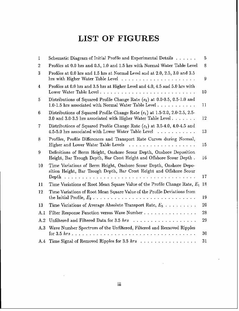
LIST OF FIGURES

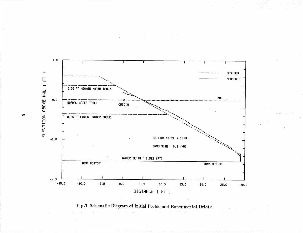
1 Schematic Diagram of Initial Profile and Experimental Details . . . . . . 5

2 Profiles at 0.0 hrs and 0.5, 1.0 and 1.5 hrs with Normal Water Table Level 8

3 Profiles at 0.0 hrs and 1.5 hrs at Normal Level and at 2.0, 2.5, 3.0 and 3.5hrs with Higher Water Table Level ................... .. 9

4 Profiles at 0.0 hrs and 3.5 hrs at Higher Level and 4.0, 4.5 and 5.0 hrs withLower Water Table Level ................... ...... . 10

5 Distributions of Squared Profile Change Rate (el) at 0.0-0.5, 0.5-1.0 and1.0-1.5 hrs associated with Normal Water Table Level . . . . . . . . ... 11

6 Distributions of Squared Profile Change Rate (el) at 1.5-2.0, 2.0-2.5, 2.5-3.0 and 3.0-3.5 hrs associated with Higher Water Table Level ....... .. 12

7 Distributions of Squared Profile Change Rate (el) at 3.5-4.0, 4.0-4.5 and4.5-5.0 hrs associated with Lower Water Table Level . . . . . . . . ... 13

8 Profiles, Profile Differences and Transport Rate Curves during Normal,Higher and Lower Water Table Levels. . . . . . . . . . . . . . . . . 15

9 Definitions of Berm Height, Onshore Scour Depth, Onshore DepositionHeight, Bar Trough Depth, Bar Crest Height and Offshore Scour Depth . 16

10 Time Variations of Berm Height, Onshore Scour Depth, Onshore Depo-sition Height, Bar Trough Depth, Bar Crest Height and Offshore ScourDepth ................. ................... 17

11 Time Variations of Root Mean Square Value of the Profile Change Rate, E 1 18

12 Time Variations of Root Mean Square Value of the Profile Deviations fromthe Initial Profile, E2 . . . . . . . . . . . . . . . . . . . . . . . . . .. . . 19

13 Time Variations of Average Absolute Transport Rate, E3 . . . . . . ... 20

A.1 Filter Response Function versus Wave Number . . . . . . . . . . . . .. . 28

A.2 Unfiltered and Filtered Data for 3.5 hrs . . . . . . . . . . . . . .... 29

A.3 Wave Number Spectrum of the Unfiltered, Filtered and Removed Ripplesfor 3.5 hrs . . . . . . . . . . . . . . . . . . . . . . . . . . . . . . . . . .. .. 30

A.4 Time Signal of Removed Ripples for 3.5 hrs . . . . . . . . . . . . . ... 31

:iii

1 Introduction

The swash zone is defined as that region on the beach face delineated at the upperlevel by the maximun uprush of the waves and at its lower extremity by the maximundownrush. This region becomes alternately wet and dry, as the waves move up anddown until they disappear into the beach or return to the sea. Knowledge of the swashzone is very important because not only does it provide the boundary condition forbeach profile evolution models but sediment transport in this zone is directly relatedto the shoreline position. Additionally, a significant portion of the longshore sedimenttransport may occur in the swash zone. Hence, considerable research has been directedtoward understanding and predicting swash mechanisms and related processes.

Studies by Bagnold (1940) and Bascom (1951) found that the dynamic sedimentdistribution in the swash zone is a function of the characteristics of the incoming wavesand the sand size. The effects of incoming waves are obvious; they provide the massand momentum of the water in the swash zone. On the other hand, the sand size of thebeach face is related to its stability and will influence the water motion through the bedroughness and the porosity. If we change the point of view from individual factors to theforces induced by them, then we can say that the sediment transport in the swash zoneis a function of several forces (e.g., friction, gravity, inertia and pressure gradient forces)acting on a water element within the swash zone.

With the combination of these forces, the waves rush up the foreshore until they loseall their forward momentum, at which time the velocity of the leading edge of the wavesor the mass of uprush flow is zero. During that time, most of the sediment transportedis deposited on the foreshore. As the foreshore slope is increased by sediment deposition,backrush velocities are increased thereby limiting further net acceretion. Finally, theequilibrium slope of the swash zone is reached. However, if there are any changes inthese forces, the system will again be put into disequilibrium.

Grant (1948) noted by observations that the aggradation or degradation of a beach,and the value of the beach slope are functions of several variables, one of which is theposition of the ground water table within the beach. A high water table acceleratesbeach erosion, and conversely, a low water table may result in pronounced aggradation

of the foreshore. This concept has been supported by various researchers. Most of their

studies have focused on tidal cycle response (Emery and Foster, 1948; Duncan, 1964) oron high frequency response to individual waves (Emery and Gale, 1951; Waddel, 1973and 1976; Sallenger and Richmond, 1984). The results of these studies not only supportGrant's idea very strongly but try to provide additional physical reasoning. If we have alow water table, water percolates rapidly into the sand and reduces the uprush mass aswell as velocity and this facilitates deposition of sand over the swash zone. Converselyfor a saturated beach, water escapes through the sand and increases mass and velocityof the backrush flow and this enhances erosion of the swash zone. Most of the availablestudies are based on field measurements and have not been carried out with controlledlaboratory experiments.

1

Based on possibilities of beach stabilization, test installations of the beach drainsystem have been conducted; this approach consists of burying a pipeline along thebeach to lower the water table level on the beach face by pumping (Machemehl, Frenchand Huang, 1975; Chappell, Eliot, Bradshaw and Lonsdale, 1979; Danish GeotechnicalInstitute, 1986; Terchunian, 1989). Successful demonstrations have been carried out inthe laboratory and apparently in the field, although the field data are more ambiguous.Most of these studies argued that beach dewatering stabilizes beaches by enhancingdeposition on wave uprush and retarding erosion on wave backrush and hence, beachaggradation could be induced by maintaining the beach water table at a low level.

As noted by Dean and Dalrymple (1991), however, it is not obvious how this methodworks, which it clearly does in the laboratory. Kawata and Tsuchiya (1986) pointed outthe ratio of the seepage velocities within the sand to the velocities within the jet of fluidrushing up the beach face are about 1/1000. Bruun (1989) claimed that the methodought to be more effective in mild conditions than storm conditions as the velocities arefar higher in the surf zone during a storm. It was noted also by Chappel et. al. that,in the case of beach erosion, more is involved than the simple effect of high water tablesincreasing the backrush.

This brief report presents the results of a laboratory study of beach face dynamicsas affected by the variations of ground water table elevations within the beach. Toachieve this goal, an experiment was conducted at three different water table levels whilethe other factors (e.g., wave height, wave period, water depth, initial beach slope, etc.)were fixed to constant values with regular waves. The water table levels included : (a)normal water table level which is the same as mean sea level, (b) a higher level and (c)a lower level than the mean sea level. Special attention is given to the higher water levelto investigate whether this level enhances erosion of the beach face or not and also tomethods of interpreting the experimental data.

2 Laboratory Studies

2.1 Facilities

Laboratory studies were carried out in the Coastal and Oceanographical EngineeringLaboratory to investigate the effects of ground water table elevations on the beach profilechanges over the swash zone. The major facility was a wave tank which is 120 ft long, 6ft wide and 6 ft deep. A long partition has been constructed along the tank centerlinedividing it into two channels each of 3 ft width. A hydraulic driven piston-type wavemaker is located at one end of tank and a sand beach was constructed at the downwaveend of the parallel channel in which the tests were conducted. Regular waves with aperiod of 2.0 sec and height of 0.160 m were utilized for this experiment. The initialbeach profile was linear at a slope of 1:18. The water depth at the toe of the beach slopewas 1.5 ft at mean sea level. The beach was composed of well-sorted fine sand with amedian diameter of 0.2 mm (2.32 in 0 unit) and a sorting value of 0.53.

2

2.2 Procedures

The experiment was conducted over a duration of 4.5 hrs to examine the changes ofan initially linear beach profile subject to a regular wave at three different water tablelevels. The duration of each test with the same water table level was determined based onan assessment that the beach profiles were near equilibrium and would not significantlychange beyond this test duration. Throughout the test program, the beach profiles weremonitored at one-half hour intervals.

The test procedures are as followings:

1. Measure the initial beach profile.

2. Run waves for 1.5 hrs with normal water table level.

3. Establish a new water table level which is 0.36 ft higher than normal.

4. Run waves for 2.0 hrs while maintaining the higher water table level.

5. Establish a new water table level which is 0.36 ft lower than normal.

6. Run waves for 1.5 hrs while maintaining the lower water table level.

The raised water table (at 1.5 hrs) was established by raising the entire water level inthe wave tank and allowing the ground water table to equilibrate with no waves acting.The tank water level was then lowered and the water table was maintained by excavatinga small depression in the berm below the desired water level, which was then maintainedby filling periodically with a hose. For the lower water table, the procedure describedabove was followed except that water was siphoned out of the excavated hole in the beachberm to maintain the desired level.

2.3 Measurements

For two-dimensional laboratory experiments, sand should be conserved between a land-ward position of profile closure, where no changes in profile occurred, and a seawarddepth of closure, where no sand transport occurred; this implies that the profile datameasurements should cover the length between these two positions.

During the experiment, the landward closure could be defined easily by observation.However, defining the seaward depth of closure was more difficult since a small quantityof sand was transported beyond the toe of the beach slope and was spread in a thin layerover the horizontal section of the tank. Hence, the seaward closure was assumed to belocated at 1 ft seaward from the toe of beach. These allowances of the small seawardtransport could cause transport volume errors, which will be discussed later.

3

In this study, the origin is taken at the landward position of profile closure and atstill water level, with the x-axis oriented seaward and the z-axis upward. For this origin,the seaward depth of closure was found to be approximately 30 ft and this length isdesignated as £. Fig.1 shows the schematic diagram of initial profile and experimentaldetails.

Beach profiles over a 30.0 ft portion of the active profiles were documented by acombination of automatic bed profiler which only functions over submerged profiles andmanual measurements at time intervals of 0.5 hrs. The profiler mounted on the carriagewas used for measuring the beach profiles from 7.0 ft to 30.0 ft. The beach profilefrom 0.0 ft to 7.0 ft was measured manually since the water depth in this region wastoo small for accurate readings. Exceptions are the profiles at 0.0 and 1.5 hrs. Forthe initial profile, the whole profile over the measurement length was measured by usingprofiler after increasing the mean sea level. The profile at 1.5 hrs was documented byusing the profiler except for the landward 1.0 ft portion. These two parts of bed profiledata were combined later for subsequent processing. In addition, three profiles across thetank were measured over the whole measurement length to document three-dimensionaleffects; these three profiles were averaged to represent the mean profile. It is noted thatthe profiler did not operate properly during the profile measurements at 3.0 and 3.5 hrsand only one profile was taken at these times. It should be noted also that the offsetof profiler changed approximately 0.04 volt after 3.0 hrs, which could cause the shift ofbed profile as much as 0.03 ft. The effects of these errors in the measurements will bediscussed in the next section.

3 Data Analysis

3.1 Compilation of Data

Sand conservation can be checked easily by calculating the time-averaged change in sed-iment volume per unit width of tank, which is obtained by integrating the profile differ-ences from the initial profile over the portion of the active profiles as :

V(t)=- [z(x,t) - z(x,0)] dx (1)

here z(x, t) is the profile elevation at a given point x and time t and z(x, 0) is the initialprofile.

For complete conservation of sand, if the bulk density is unchanged, the integratedvalue V(t) should be zero. However, as expected, the errors in transport volumes werefound to be non-zero. To satisfy the condition of sand conservation the mean profile ateach time step was adjusted. The details of this adjustment and a filtering procedure toremove the ripples are summarized in Appendix A.

4

1.0 IIIIII

..------------ DESIRED-.........--.........--..........

ESURE- -MEASUREDu-

0.36 FT HIGHER WATER TABLE

MWL

NORMAL HATER TABLE ORIGIN

§ - TA- -CDZ 0.36 FT LOWER HATER TABLEC

-I

SINITIAL SLOPE = 1:18-1.0

SAND SIZE = 0.2 (MM)

WATER DEPTH = 1.542 (FT)

TANK BOTTOM' TANK BOTTOM

-2.0 I I I I I I

-15.0 -10.0 -5.0 0.0 5.0 10.0 15.0 20.0 25.0 30.0

DISTRNCE ( FT )

Fig.1 Schematic Diagram of Initial Profile and Experimental Details

3.2 Equilibrium Criteria

For analyzing the data, it is helpful to define what is meant by 'equilibrium' profileand also to determine whether or not equilibrium has been reached. In the field, theequilibrium profile is considered to be 'dynamic' as the tide and incident wave field changecontinuously in nature and therefore the profile changes shape as well. In the laboratoryit is relatively easy to establish an equilibrium profile, by running a steady wave train ontoa beach for a long time. After the remolding of the initial profile, a 'final' profile results,which changes little with time. This is the equilibrium profile for that beach materialand wave conditions. Hence, as a beach profile approaches an equilibrium, the incidentwave energy is dissipated without any significant profile changes and the time-averagedsediment transport rate converges to zero at all points along the profile.

From this definition of equilibrium, we can develop criteria to indicate the approachof the profile to an equilibrium. In this study, three criteria are suggested as follows :

(1) Root mean square (RMS) profile change rate, E1

E1 el(x, t) d (2)

where,el(,t) = (AZ)2Az = z(x,t) - z(x,t - At) (3)At = the profiling interval ( 0.5 hrs )

E1 has dimensions of velocity and indicates the rate of profile change during consecutivetimes.

(2) RMS profile deviations from initial profile, E2

E2 = e2(x, t) dx (4)

where,e2(x,t) = [z(x,t) - z(x, 0)2 (5)

E 2 has dimensions of length and indicates the overall profile changes relative to theinitial profile. As the profile approaches equilibrium, E2 approaches a constant value,which implies that the decrease in slope of the E 2 curve is a measure of the rate atwhich the equilibrium is approached. This criterion may be misleading as a measure ofequilibrium as it can be seen that a profile shifting along an initially planar slope wouldcause no change in E2. Hence, it may not be a good measure.

6

(3) Average of the absolute transport rate, E3

lfoE3 = e3 (x, t) dx (6)

where,e3(x,t) = |q(x,t)lq(x, t) = time-averaged sediment transport rate (7)

= -fo dx

E3 has dimensions of transport rate per unit width of tank. This criteria is equal to theaveraged sediment transport rate over the interval of change. Also, E3 approaches zerowith equilibrium conditions.

Smaller values of criteria E1 and E3 and steady values of criteria E2 indicate thatthe profile is more stable and approaches an equilibrium. If there are any changes inexperimental conditions such as variations in water table level, then we would expect thethree criteria to reflect these changes.

4 Results and Discussions

The profile evolutions with three water levels are presented in Fig.2 through Fig.4. Fig.2shows the profiles at 0.0, 0.5, 1.0 and 1.5 hrs measured during normal water table level.Fig.3 and Fig.4 show the profiles measured during higher and lower level, respectively,together with the initial profile and the last profile of the previous water table level. Ingeneral, the bar moved seaward with normal level, and the profiles were approaching anequilibrium. After changing to the higher level, the bar started to move landward rapidlyat the initial stages and stayed stationary at the later times. Also at the higher watertable, the trough deepened and the profile aggraded substantially in a zone immediatelylandward of the trough. The bar position remained almost fixed even after lowering thewater table level. Profile changes in the swash zone were small during the normal andlower water table levels. However, the berm built up very rapidly during the higher level.

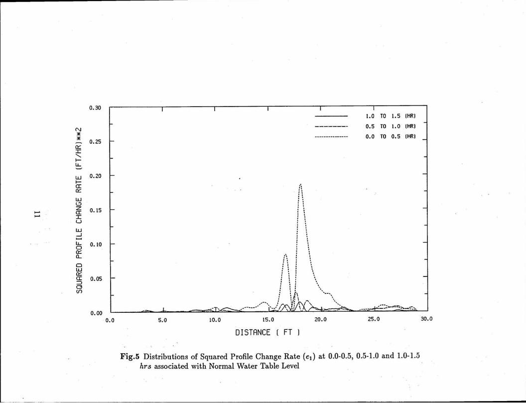
These general trends can be confirmed more clearly by examining Fig.5 through Fig.7,which represent the distributions of the squared profile change rate over the measurementlength with the fixed water table level. Fig.5 shows the squared values at 0.0-0.5, 0.5-1.0and 1.0-1.5 hrs with normal level while Fig.6 and Fig.7 show the distributions with thehigher and lower level. During the first wave run, shown in Fig.5, significant changesoccurred as the profile shape varied from a nearly planar slope to a barred profile. Asthe profile approached equilibrium, the values of the distributions approached zero at allpoints. As soon as the higher level was established, however, very large changes occurredat the bar crest with relatively smaller changes at the bar trough.

7

1.0 I

1.5 (HR)

- - 1.0 (HR)LL 0.5

S------- 0.5 (HR)

j ------------- 0.0 (HR)

C -0.5 --I--

a:

._J

-1.0 - -

-1.5

-2.00.0 5.0 10.0 15.0 20.0 25.0 30.0

DISTANCE [ FT I

Fig.2 Profiles at 0.0 hrs and 0.5, 1.0 and 1.5 hrs with Normal Water Table Level

1.0 I

3.5 (HR)

-- -- 3.0 (HR)

.- - --- - 2.5 (HR)L.. 0.5

2.0 (HR)

_j ------ 1.5 (HR)

S-- -...--..- ----. 0.0 (HR)S0.0.0 -- R]

S0.0

o -0.5

-j

1.0

-1.5

-2.0 I I

0.0 5.0 10.0 15.0 20.0 25.0 30.0

DISTANCE ( FT ]

Fig.3 Profiles at 0.0 hrs and 1.5 hrs at Normal Level and 2.0, 2.5, 3.0 and 3.5 hrs withHigher Water Table Level. Note the rapid build-up above the mean water level(MWL) and scour below MWL.

1.0

5.0 (HR]

- -- --- 4.5 (HR)L- 0.5

4.0 (HR)

_------ 3.5 (HR)

-I- . ... 0.0 (HR)

. 0.0 -------------------------------------------

O -z HWL

O -0.5

_J

-i.S-1.0

-1.5

-2.00.0 5.0 10.0 15.0 20.0 25.0 30.0

DISTANCE ( FT

Fig.4 Profiles at 0.0 hrs and 3.5 hrs at Higher Level and 4.0, 4.5, and 5.0 hrs with

Lower Water Table Level. Note the relatively small changes.

0.30

1.0 TO 1.5 (HR)

S-------- 0.5 TO 1.0 (HR)

----- 0.0 TO 0.5 (HR)0.25

I-i-

Ll 0.20-CE

S'a

LUa ;

z 0.15 -

U

Q-

LL

0.0

0.00 T h ; \O.00 a"- " * -a"»--.... ""/ ': " - ^-"----- -----

0.0 5.0 10.0 15.0 20.0 25.0 30.0

DISTANCE ( FT

Fig.5 Distributions of Squared Profile Change Rate (el) at 0.0-0.5, 0.5-1.0 and 1.0-1.5hrs associated with Normal Water Table Level

0.30 I I

3.0 TO 3.5 (HR)

- - - - 2.5 TO 3.0 (HR)

0.--- - 2.0 TO 2.5 (HR)0.25 -

Q ------------- 1.5 TO 2.0 (HR)r

I-LL-

LU 0.20

1-

N 2 0.15

cI- 0 . 10 -

C3

fo I

S0.000.0 5.0 10.0 15.0 20.0 25.0 30.0

DISTANCE ( FT )

Fig.6 Distributions of Squared Profile Change Rate (el) at 1.5-2.0, 2.0-2.5, 2.5-3.0 and3.0-3.5 hrs associated with Higher Water Table Level

0.30 I

4.5 TO 5.0 (HR)

S---- - 4.0 TO 4.5 (HR)

S------ -- 3.5 TO 4.0 (HR)0.25

ILCr

Ll 0.20

0..

(-i

(L(.3

ISTNCE ( FT (

UJ

-1

C 0.105Q-

0.00.-0 ..... ... ..-*- h * -- =,=- l,----,--.~- "•, • .,.• ._= .. _, - .- --./ -*^ ^ - -- -- - "" - " --

0.0 5.0 10.0 15.0 20.0 25.0 30.0

DISTRNCE ( FT

Fig.7 Distributions of Squared Profile Change Rate (el) at 3.5-4.0, 4.0-4.5 and 4.5-5.0hrs associated with Lower Water Table Level

Also, significant deposition commenced within the upper portion of the swash zone.During the experiment with the higher water level, the peak of the berm moved landwardcontinuously, which meant deposition over the swash zone. This is contradictory to pre-vious studies that higher water table level enhances erosion. However, there was erosionimmediately seaward. It appears that this eroded material was deposited landward inthe berm. As shown in Fig.7, little changes occurred with lower water table level.

Fig.8 shows the profiles, profile differences and transport rates during normal, higherand lower water table levels. We can see easily from the transport rate curves thatduring normal water level, sand was transported both onshore and offshore resulting indeposition at the berm and at the bar. During higher water table, sand was transportedonshore and deposited at the berm and at the depositional area located immediatelylandward of the bar trough. Also it can be seen that relative small changes occurredwith lower water table level.

Fig.9 shows the definition of berm height, onshore scour depth, onshore depositionheight, bar trough depth, bar crest height and offshore scour depth. All these variablesare relative to the initial profile. A negative sign denotes erosion while a positive signifiesdeposition. The time variations of these variables are shown in Fig.10, which clearlydemonstrates the features mentioned above.

The time variations of the three criteria, El, E 2 and E 3, are shown in Fig.11 throughFig.13, respectively. El is the integrated value of the squared profile change rate, shown inFig.5 to Fig.7. The value of El increases by approximately a factor of three immediatelyafter changing to a higher water table level. During higher water level, another peakvalue appears. This is because only one profile was measured at 3.0 and 3.5 hrs and themeasured one represents the highest part across the tank. During lower water table level,the variation shows that the profile remains in approximate equilibrium. The plots of E 2

and E 3 are in general agreement with the interpretation derived from E 1.

5 Conclusions

The experiment described herein was carried out with a fairly fine sand and has demon-strated the significance of beach water table on profile dynamics. Specific effects whichhave been clearly demonstrated by this experiment and recommendations for additionalexperiments are described below.

The increased water table caused distinct effects in three definite zones. First, erosionoccurred at the base of the beach face and the sand eroded was carried up and depositedon the upper portion of the beach face. This resulted in a " hinge point " at aboutthe mean water line. Secondly, the trough deepened considerably and rapidly and theeroded sand was deposited immediately landward. This depositional area changed frommildly erosional to strongly depositional. Third, the area seaward of the bar eroded witha substantial deepening. These effects are evident through inspection of Fig.2 and Fig.3(before and after water table increased, respectively).

14

1.0 i I - I I 1.0 I i I 1.0 I i

---- 0.0 (HR ---- 1.5 (HR ---- 3.5 (HR

-- 1.5 (HR - 3.5 (HR - 5.0 (HR

S0.0 ML 0.0 - -L 0.0 --

c: -1.0. -. O -0S-1.0 - - -1.0 - - -. -

-2.0 -2.0 I -2.00. 10. 20. 30. 0. 10. 20. 30. 0. 10. 20. 30

0.3 1 I I I 0.3 1 I I I 0.3 I I

-0.3 -0.3 -0.3

0. 10. 20. 30. 0. 10. 20. 30. 0. 10. 20. 30

1.0 - I | - 1 I I 1.0 I 1.0 I I - -I

I-

0 0.5 - 0.5 - - 0.5 -

-i

C- 0.0 0.0 - - - - - -0.0 0.0

-O. - -0.5 -0.5 -

-1.03 -. I -1.0

0. 10. 20. 30. 0. 10. 20. 30. 0. 10. 20. 30

DISTANCE ( FT ) DISTANCE ( FT ) DISTANCE ( FT )

(a) NORMAL WATER TABLE (b) HIGHER WATER TABLE (c) LOWER WATER TABLE

Fig.8 Profiles, Profile Differences and Transport Rate Curves during Normal, Higherans Lower Water Table Levelsans Lower Water Table Levels

ZBH

Berm

DepositionalArea

ZOS Bar

ZOD

Initial

ZBC Profile

ZBT

ZOF

Fig.9 Definitions of Berm Height, Onshore Scour Depth, Onshore Deposition Height,

Bar Trough Depth, Bar Crest Height and Offshore Scour Depth

NORMAL W.T.L. HIGHER W.T.L. LOWER W.T.L.0.7 1 1 I 1 I 1 I

S ------ *----- ZBH :BERM HEIGHT

0.6 - -----.------- ZOS :ONSHORE SCOUR DEPTH

------- ------- ZO : ONSHORE DEPOSITION

0.5 I ZBT : BRR TROUGH DEPTH

----- ZBC : BAR CREST HEIGHTLL

0.4 - ZOF : OFFSHORE SCOUR DEPTH

- 0.3 -LL!

CE 0.2

I L~~~~- ------- - - - - - - - - - - - - - - - - - - - - - - - - - - --- I i-- , ------- ------t J- I .... ......... • . .....-.---- "'"" , ..

CI .- ....- ---- I.z ..... .. -I .- +---

0 -------------::: ..... ..-- ---' .---- -------- - - - ------ --- - - - - -- - ---- ---- - -- --- -- --

> 0. -_l- - -------------- -"-.---LL -0.1

-0.2

-0.30.0 0.5 1.0 1.5 2.0 2.5 3.0 3.5 4.0 4.5 5.0

TIME ( HOUR )

Fig.10 Time Variations of Berm Height, Onshore Scour Depth, Onshore DepositionHeight, Bar Trough Depth, Bar Crest Height and Offshore Scour Depth

NORMRL W.T.L. HIGHER W.T.L. LOWER W.I.L.

0.2 1

C:I-

LL

I-

_): 0.

0.0 0.5 1.0 1.5 2.0 2.5 3.0 3.5 4.0 4.5 5.0

CI_

-J

0.0 I I I III__

0.0 0.5 1.0 1.5 2.0 2.5 3.0 3.5 4.0 4.5 5.0

TIME ( HOUR

Fig.ll Time Variations of Root Mean Square Profile Change Rate, E1

NORMAL W.T.L. HIGHER W.T.L. LOWER W.T.L.

0.2 I I

I-

bJ

UJ

U-

0.1

LU

cr,

a-

0

of(I)

0: 0.

0.0 0.5 1.0 1.5 2.0 2.5 3.0 3.5 4.0 4.5 5.0

TIME ( HOUR )

Fig.12 Time Variations of Root Mean Square of Profile Deviations from Initial Profile, E2

NORMRL W.T.L. HIGHER W.T.L. LOWER W.T.L.0.2 I I I I I

.- -LL1

I.--

U-

LLI

cI

o 0.0

0.0 0.5 1.0 1.5 2.0 2.5 3.0 3.5 4.0 4.5 5.0

TIME ( HOUR

Fig.13 Time Variations of Average Absolute Transport Rate, E3Fig. 13 Time Variations of Average Absolute Transport Rate, £'3

It is somewhat surprising that the increased water table was effective so far offshore.The common effect responsible for the changes in the three zones appears to be a destabi-lization of the bottom particles in areas of pre-existing marginal stability with the erodedparticles transported to stable areas. The lowered water table appeared to result in amuch more stable beach and the resulting effects were much less. The only noticeabletrend was a limited deposition in the scour hole at the base of the beach face (Fig.4).

There is a substantial need for additional carefully controlled laboratory experiments.It is anticipated that results may differ substantially with sediment characteristics andthus experiments should encompass a range of sizes (and thus permeabilities) and sorting.Improved monitoring of the distribution of the ground water table elevations throughoutthe beach berm as well as the piezometric head within the beach across the surf zoneshould be considered. The temporal (wave period scale) small scale water table changesas the wave front rushes up and down the beach face should be documented for a rangeof sand size characteristics. Differences for irregular waves and regular waves as investi-gated here should be investigated. Finally, all comprehensive studies should include atleast limited experiments to document repeatibility and experiments to provide controlsillustrating beach profiles that would have occurred if the water tables had not beenaltered.

6 References

Bagnold, R.A. (1940), " Beach Formation by Waves; Some Model Experiments in aWave Tank ", Inst. Civil Engineers Jour., Paper No. 5237, pp 27-53.

Bascom, W.N. (1951), " The Relationship between Sand Size and Beach Face Slope ",American Geophysical Union Transactions, 32(6), pp 866-874.

Bruun, P. (1989), " Coastal Drain: What Can It Do or Not Do? ", J. Coastal Research,5(1), pp 123-125.

Chappell, J., I.G. Eliot, M.P. Bradshaw and E. Lonsdale (1979), " Experimental Controlof Beach Face Dynamics by Water-Table Pumping ", Engineering Geology, 14, pp29-41.

Danish Geotechnical Institute (1986), " Coastal Drain System: Full Scale Test-1985Tormindetangen ", June.

Dean, R.G. and R.A. Dalrymple (1991), " Coastal Processes with Emphasis on En-gineering Applications ", unpublished draft text for Graduate Course EOC 6196:Littoral Processes, Department of Coastal and Oceanographic Engineering, Uni-versity of Florida, Gainesville, Florida.

21

Duncan, J.R. (1964), " The Effect of Water Table and Tide Cycle on Swash-BackwashSediment Distribution and Beach Profile Development ", Marine Geology, 2, pp186-197.

Emery, K.O. and J.F. Foster (1948), " Water Tables in Marine Beaches ", J. MarineResearch, 7, pp 644-654.

Grant, U.S. (1948), " Influence of the Water Table on Beach Aggradation and Degra-dation ", J. Marine Research, 7, pp 655-660.

Kawata, Y. and Y. Tsuchiya (1986), " Application of Sub-Sand System to Beach ErosionControl ", Proc. International Coastal Engineering Conference, ASCE, Taiwan, pp1255-1267.

Machemehl, J.L., French, T.J. and Huang, N.E. (1975), " New Method for Beach Ero-sion Control ", Proc. Civil Engineering in the Oceans, III, ASCE, University ofDelaware, pp 142-160.

Sallenger, A.H., Jr. and B.M. Richmond (1984), " High- Frequency Sediment-LevelOscillations in the Swash Zone ", in Hydrodynamics and Sedimentation in Wave-Dominated Environments, ed. by B. Greenwood and R.A. Davis, Jr., Marine Ge-

ology, 60, pp 155-164.

Terchunian, A.V. (1989), " Performance of the STABEACH@ System at HutchinsonIsland, Florida ", Proc. Beach Preservation Technology 89, University of Florida,Florida Shore and Beach Preservation Association and the American Shore andBeach Preservation Association, Tampa, Fl., pp 229-238.

Waddel, E. (1973), " Dynamics of Swash and Implication to Beach Response ", CoastalStudies Institute, Louisiana State University, La., Technical Report No. 139, 49

pp.

Waddel, E. (1976), " Swash-Groundwater-Beach Profile Interactions ", in Beach andNearshore Sedimentation, ed. by Davis, R.A. and R.L. Ethington, Society of Eco-nomic Paleontologists and Mineralogists, Special Publication No. 24, pp 115-125.

22

APPENDIX A

DATA REDUCTION

In this appendix, the possible causes of errors in transport volumes are discussedat first in an attempt to provide a reference for future experiments. Next the methodis presented to adjust the experimental data to remedy these errors within resonablelimits.

The errors in transport volumes and mismatch at the point of manual and profilermeasurement are believed to be caused by combinations of following :

(1) three-dimensional effects

(2) the small amount of sand that was transported seaward of the measurement limit

(3) consolidation of the sand under the beach

(4) change of profiler offset after 3.0 hrs

The errors from (1), (2) and (3) may be inherent in most of movable bed experiments,while the error (4) is confined to this experiment.

Three-dimensional effects can be removed by measuring several profiles along thelines parallel to the axis of the tank. In this experiment, three profiles were measuredacross the tank, which were averaged to represent the mean profile. However, at 3.0and 3.5 hrs the profile along only one line was measured. Hence three-dimensionaleffects can be important for these two times. Due to the non-zero water particle velocityover the horizontal section of tank bottom, sand was transported beyond the seawardmeasurement limit and was spread over the horizontal-floor of the tank. During theexperiment, no significant sand volumes were observed. Thus it appears that theseerrors are negligible. The effect of sand consolidation may be important as the sandwithin the beach becomes more compact under continued wave action. At the presenttime, however, there are no avilable means to consider the effects of sand consolidation.

As noted, it was found that in the overlap region in which the profile was obtained byboth the profiler and manually, there was a mismatch of elevations. In this experiment,the manual measurements were used as one basis for calibrating the profiler. Laterinspection of the data suggested that after 3.0 hrs, the profiler calibration changedconsiderably. The basis for post-calibrating the profiler for each run was to matchthe profiles in the overlap region to the manual readings and to require that the totalvolumetric changes were zero.

23

The calibration relationship between the elevation, z,, and the output v of the profileris

z,(x,t) = a + b v(x,t) - WL (A.1)

where,

z(x, t) = calibrated profile elevation (ft)

v(x,t) = profiler data (volt)

a = calibration offset (ft)

b = calibration slope (ft/volt)

WL = water depth to shift the origin from the tank

bottom to the water level (ft)

For this experiment, the profiler was calibrated based on the initial profile and theresults were

a = 3.748362 (ft)

b =- 0.738907 (ft/volt)

With these constants, transport volume errors and mismatch are found as summa-rized in Table A.1. For each run, the calibration was redetermined so that the profilerresults provided;

(1) agreement over the range of manual profiles, and

(2) zero total volume changes.

If we express the bed profile data as

(x) zm (x,t) ,0 < x < (A.2)

zp (X, t) , xz < X < _

where,

z,(x, t) = manual data at x(ft)zp(x,t) = profiler data at x(ft)

= (a + Aa) + (b + Ab)v(x,t) - WLAa(t) = correction in calibration offset (ft) (A.3)Ab(t) = correction in calibration slope (ft/volt)Xl = x position of a matching point£ = total measurement length ( 30 ft )

24

Table A.1: Volume Errors and Mismatch

Time Transport Volume Mismatch

(hr) (ft 2) x,(ft) Az(ft)0.5 -0.0508 7.0 0.00901.0 -0.0682 7.0 0.02241.5 -0.1060 1.0 0.00882.0 -0.0503 7.0 0.02832.5 -0.0727 7.0 0.01263.0 -0.4238 7.0 -0.01423.5 1.3318** 7.0 0.08954.0 1.4139 7.0 0.07724.5 1.6570 7.0 0.10165.0 1.4291 7.0 0.0828

* A positive Az denotes the elevation by theprofiler is below that determined manually.

** After three hours, a significant change in profilercalibration apparently occurred.

then, we can set up two objective equations.

i) continuity at the matching point xz

Az(x 1) = zm(xx,t) - Zp(x 1 ,t) = 0 (A.4)

ii) zero volume error

AV(t) = [z(x,t) - z(x,0)] dx = 0 (A.5)

z(x, 0) = initial profile dataS c+dv(x,0)- WL (A.6)

c = 3.748362 (ft)d =- 0.738907 (ft/volt)

Based on the above, we can develop simultaneous equations for Aa and Ab as follows:

A 1Aa + BAb = C (.A 2Aa + B 2Ab = C2 (

25

Table A.2: Calibration Factors at Each Time Step

Time Slope Offset(hr) (ft/volt) (ft)0.0 -0.738907 3.748360.5 -0.753827 3.804411.0 -0.773760 3.881591.5 -0.752734 3.795712.0 -0.780490 3.908842.5 -0.760062 3.827903.0 -0.745610 3.755213.5 -0.779667 3.972094.0 -0.756362 3.882634.5 -0.774138 3.965625.0 -0.762894 3.90967

where,

A 1 = - xl

B, = v(x,t) dx1

C1 = C1 + C12 + C13 + C14 + C15

C11 = (c - WL)xi

C12 = (c - a)Ai

C 1 3 = d v(x,0) dx

Cl4 = - Zm(x, t) dx

C15 = -bB 1

A2 = 1.0

B 2 = v(x 1,t)

C2 = z,(x, t) -[(a- WL) + bv(xi,t)]

The final calibration factors are summarized in Table A.2.

26

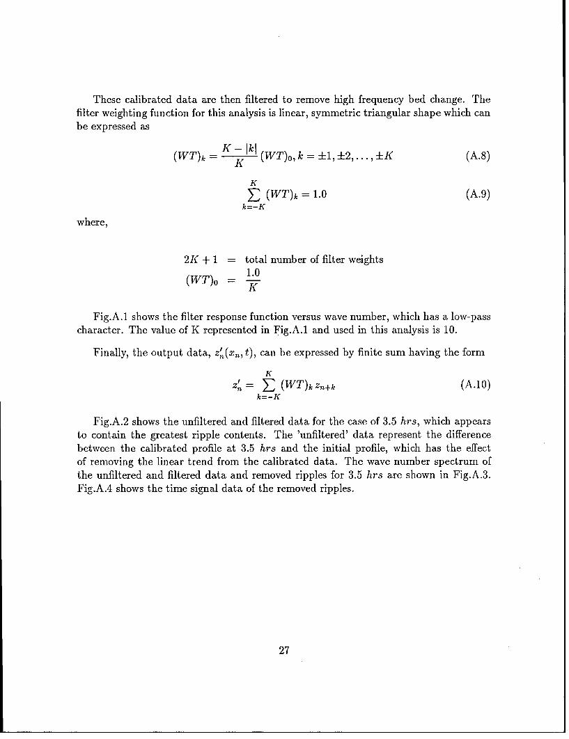
These calibrated data are then filtered to remove high frequency bed change. Thefilter weighting function for this analysis is linear, symmetric triangular shape which canbe expressed as

(WT)k = K- (WT)o, k = ±1,±2,..., ±K (A.8)K

E (WT)k = 1.0 (A.9)k=-K

where,

2K + 1 = total number of filter weights1.0

(WT)o =

Fig.A.1 shows the filter response function versus wave number, which has a low-passcharacter. The value of K represented in Fig.A.1 and used in this analysis is 10.

Finally, the output data, z,(x,, t), can be expressed by finite sum having the form

K

z4 = E (WT)k Z+k (A.10)k=-K

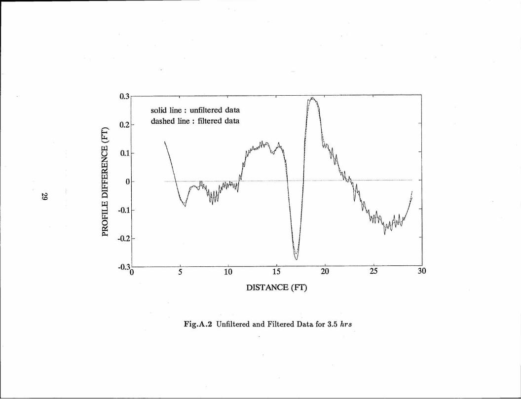
Fig.A.2 shows the unfiltered and filtered data for the case of 3.5 hrs, which appearsto contain the greatest ripple contents. The 'unfiltered' data represent the differencebetween the calibrated profile at 3.5 hrs and the initial profile, which has the effectof removing the linear trend from the calibrated data. The wave number spectrum ofthe unfiltered and filtered data and removed ripples for 3.5 hrs are shown in Fig.A.3.Fig.A.4 shows the time signal data of the removed ripples.

27

0.9

O 0.8

I °0.7-

0.6

Z 0.5

^ 0.4-

SP 0.3-

I 0.2

0.1

0 0.5 1 1.5 2 2.5 3 3.5 4

1 / WAVE LENGTH (1/FT)

Fig.A.1 Filter Response Function versus Wave Number

0.3 -

solid line : unfiltered data

0.2 dashed line : filtered data

U 0.1-

'• -o.1

0

-0.2

-0.20 5 10 15 20 25 30

DISTANCE (FT)

Fig.A.2 Unfiltered and Filtered Data for 3.5 hrs

101

solid line : unfiltered data100 + - dash line : filtered data

* - dot line : ripples

• 10-1-

S10-2-10-3

Z • ' "

' - X *. ÷

wo ~ §~ ~10-3 -b m v

0- 0.2 04 0.6 0.8 1 1.2 1.4 1.6 1.8 2

* ** i\

1 / WAVE LENGTH (1/FT)

10- *1

Fig.A.3 Wave Number Spectrum of the Unfiltered and Filtered Data and Removed

1 Ripples for 3.5 h

10-60 0.2 0.4 0.6 0.8 1 1.2 1.4 1.6 1.8 2

1 / WAVE LENGTH (1/Fr)

Fig.A.3 Wave Number Spectrum of the Unfiltered and Filtered Data and RemovedRipples for 3.5 hrs

0.04

0.03

° I I"Iz 0.02 I

0.01i

0- .

L a I ' i-0.01-

O -0.02

-0.03

040 5 10 15 20 25 30

DISTANCE (FT)

Fig.A.4 Time Signal of Removed Ripples for 3.5 hrs