Stefan Edelkamp

BDDs for Minimal Perfect Hashing: MergingTwo State-Space Compression Techniques

May 4, 2017

Springer

This work will merge two different lines of research, namely

a) state-space exploration with binary decision diagrams (BDDs), that was initially proposed for ModelChecking and still is state-of-the-art in AI Planning.

b) state-space compaction with (minimal) perfect hashing, which is used in the algorithm community as amemory-based index for big data (often residing on disk).

We will see how BDDs can serve as the internal representation of a perfect hash function with linear-time ranking and unranking, and how it can be used as a static dictionary and an alternative to the recentcompression schemes exploiting hypergraph theory. This will also result in a simple method to split a BDD inparts of equal number of satisfying assignments and to generate random inputs for any function representedas a BDD. As a surplus, the BDD-based hash function is monotone.

In terms of applications, symbolic exploration with BDD constructs a succinct representation of the statespace. For each layer of the search, a BDDs is generated and stored, and will later serve as an index to doextra work like the classification of game states. Based on this approach we will show, how to strongly solva game in a combination of symbolic and explicit-state space exploration.

We propose efficient methods for solving combinatorial problems by mapping each state to a unique bit inmemory. To avoid collisions, perfect hash functions serve as compressed representations of the search spaceand support the execution of exhaustive search algorithms like breadth-first search and retrograde analysis.

Perfect hashing computes the rank of a state, while the inverse operation unrank reconstructs the stategiven its rank. Efficient bitvector algorithms are derived and generalized to a larger variety of games. Westudy rank and unrank functions for permutation games with distinguishable pieces, for selection gameswith indistinguishable pieces, and for general reachability sets. The running time for ranking and unrankingin all three cases is linear in the size of the state vector.

To overcome space and time limitations in solving games like Frogs-and-Toads and Fox-and-Geese, weutilize parallel computing power in form of multiple cores on modern central processing units (CPUs) andgraphics processing units (GPUs). We obtain an almost linear speedup with the number of CPU cores. Dueto the much larger number of cores, even better speed-ups are achieved on GPUs.

We also combine bitvector and symbolic search with BDDs that compactly represent state sets. The hybridalgorithm for strongly solving general games initiates a BDD-based solving algorithm, which consists of aforward computation of the reachable state set, possibly followed by a layered backward retrograde analysis.If the main memory becomes exhausted, it switches to explicit-state two-bit retrograde search. We takeConnect Four as a case study.

Introduction

Strong computer players for combinatorial games like Chess or Go have shown the impact of advancedsearch engines. For many games they play on expert level, sometimes even better. For some games likeCheckers the solvability status of the initial state has been computed: the game is a draw, assuming optimalplay of both players.

We consider strongly solving a game in the sense of creating an optimal player that returns the best movefor every possible state. After computing the game-theoretical value of each state, the best possible actionis selected by looking at the values of all successor states. In many single-agent games the value of a gamesimply is its goal distance, while for two-player games the value is the best possible reward assuming thatboth players play optimally.

We apply perfect hashing, where a perfect hash function is a one-to-one mapping from the set of statesto some set {0, . . . ,m− 1} for a sufficiently small number m. Ranking maps a state to a number, while

2

unranking reconstructs a state given its rank. One application of ranking (and unranking) functions is tocompress (and decompress) a state.

We will see that for many games, space-efficient perfect hash functions can be constructed prior the search.In some cases it is even possible to devise a familiy of perfect hash functions, one for each (forward orbackward) search layer. We propose linear time algorithms for invertible perfect hashing for

• permutation games, i.e., games with distinguishable pieces. In this class we find Sliding-Tile puzzles withnumbered tiles, as well as Top-Spin and Pancake problems. The parity of a permutation will allows torestrict the range of the hash function. There are other games like Blocksworld that belong to this group.

• selection games, i.e., games with indistinguishable objects. In this class we find tile games like Frogs-and-Toads, as well as strategic games like Peg-Solitaire and Fox-and-Geese. There are other games likeAwari, Dots-and-Boxes, Nine-Men-Morris, that can be mapped to this group.

For analyzing the state space, we utilize a bitvector that covers the solvability information of all reachablestates. Moreover, we apply symmetries to reduce the time- and space-efficiencies of our algorithms. Besidesthe design of efficient perfect hash functions that apply to a wide selection of games, we compute successorsstates on multiple cores on the central processing unit (located on the motherboard) and on the graphicsprocessing unit (located on the graphics card).

For general state spaces, we look at explicit-state and symbolic hashing options that apply once the statespace is generated. As an example, BDD perfect hashing is applied to strongly solve Connect Four.

Perfect Hashing

A hash function h is a mapping of a universe U to an index set {0, . . . ,m−1}. The set of reachable statesS of a search problem is a subset of U , i.e., S ⊆ U . We are interested in injective hash functions, where amapping is injective, if for all f(x) = f(y) we have x= y. A hash function h :S→{0, . . . ,m−1} is perfect, iffor all s∈ S with h(s) = h(s′) we have s= s′. The space efficiency of a hash function h : S→{0, . . . ,m−1}is the proportion m/|S| of available hash values to states.

Given that every state can be viewed as a bitvector and interpreted as a number, one inefficient design of aperfect hash function is immediate. The space requirements of the corresponding hash table are usually toolarge. An space-optimal perfect hash function is bijective. A perfect hash function is minimal if its spaceefficiency is 1, i.e., if m= |S|.

Efficient and minimal perfect hash functions allow direct-addressing a bit-state hash table instead of mappingstates to an open-addressed or chained hash table. The computed index of the direct access table uniquelyidentifies the state.

Whenever the average number of required bits per state for a perfect hash function is smaller than thenumber of bits in the state encoding, an implicit representation of the search space is fortunate, assumingthat no other tricks like orthogonal hashing apply.

Two hash functions h1 and h2 are orthogonal, if for all states s,s′ with h1(s) = h1(s′) and h2(s) = h2(s′)we have s = s′. In case of orthogonal hash functions h1 and h2, the value of h1 can, e.g., be encoded inthe file name, leading to a partitioned layout of the search space, and a smaller hash value h2 to be storedexplicitly. If the two hash functions h1 : S→ {0, . . . ,m1−1} and h2 : S→ {0, . . . ,m2−1} are orthogonal,their concatenation (h1,h2) is perfect: for two hash functions h1 and h2 and let s be any state in S, and(h1(s),h2(s)) = (h′1(s),h′2(s)) we have h1(s) = h1(s′) and h2(s) = h2(s′). Since h1 and h2 are orthogonal,this implies s1 = s2.

3

The other important property of a perfect hash function for a state space search is that the state vectorcan be reconstructed given the hash value. A perfect hash function h is inversible, if given h(s), s ∈ S canbe reconstructed. The inverse h−1 of h is a mapping from {0, . . . ,m−1} to S. Computing the hash valueis denoted as ranking, while reconstructing a state given its rank is denoted as unranking.

For the exploration of the search space, in which array indices serve as state descriptors, inversible hashfunctions are required. For the design of minimal perfect hash functions in permutation games, parity willbe a helpful concept. An inversion in a permutation π = (π1, . . . ,πn) is a pair (i, j) with 1 ≤ i < j ≤ nand πi > πj . The parity of the permutation π is defined as the parity (mod 2 value) of the number ofinversions in π, A permutation game is parity-preserving, if no move changes the parity of the permutation.Parity-preservation allows to separate solvable from insolvable states in several permutation games. If theparity is preserved, the state space can be compressed.

A property p : S → N is move-alternating, if the parity of p toggles for every action, i.e., for all s ands′ ∈ succs(s) we have p(s′) mod 2 = (p(s)+1) mod 2. As a result, p(s) is the same for all states s in oneBFS layer. States s′ in the next BFS layer can be separated by knowing p(s′) 6= p(s). One example for amove-alternation property is the position of the blank in the sliding-tile puzzle.

Bitvector State Space Search

In two-bit breadth-first search every state is expanded at most once. The two bits encode values in {0, . . . ,3}with value 3 representing an unvisited state, and values 0, 1, or 2 denoting the current search depth mod 3.This allows to distinguish generated and visited states from ones expanded in the current breadth-first layer.

It is possible to generate the entire state space using one bit per state. As it does not distinguish be-tween states to be expanded next (open states) and states already expanded (closed states), such one-bitreachability algorithm determines all reachable states but may expand a state multiple times. Additionalinformation extracted from a state can improve the running time by decreasing the number of states to bereconsidered (reopened).

For some domains, one bit per state suffices for performing breadth-first search. In Peg-Solitaire the numberof remaining pegs uniquely determine the breadth-first search layer, so that one bit per state can separatenewly generated states from expanded one. This halves the space needed compared to the more generaltwo-bit breadth-first search routine. In the event of a move-alternation property we, therefore, can performbreadth-first search using only one bit per state. One important observation is that not all visited statesthat appear in previous BFS layers are removed from the current search layer.

We next consider two-bit retrograde analysis. Retrograde analysis classifies the entire set of positions inbackward direction, starting from won and lost terminal ones. Moreover, partially completed retrogradeanalyses have been used in conjunction with forward-chaining game playing programs to serve as endgamedatabases. Retrograde analysis works well for all games, where the game positions can be divided intodifferent layers, and the layers are ordered in such a way that movements are only possible inbetween alayer or from a higher layer to a lower one. Then, it is sufficient to do the lookup in the lower layers onlyonce during the computation of each layer. Thus, the bitstate retrograde algorithm is divided into threestages: during initialization all positions that are won for one player are marked. Then, the successors aresearched in the lower layers, and, then, an iteration over the remaining unclassified positions. As a result,it is sufficient to consider only successors in the same file.

In the second part a position is marked as won if it has a successor that is won for the player to move,otherwise the position remains unsolved. Even if all successors in the lower layer are lost for one position,then this position remains unsolved. A position is only marked as lost in the third part of the algorithm,because only then it is known what all the successors are. If there are no successors in the third part, thenthe position is marked as lost.

4

Provided additional state information indicating the player to move, bitstate retrograde analysis for zero-sum games requires two bits to denote if a state is unsolved, a draw, won for the first player, or won forthe second player.

Bitstate retrograde analysis applies backward BFS starting from the states that are already decided. Forthe sake of simplicity, in our implementation we first look at two-player zero-sum games that have no draw.Based on the players’ turn, the state space is in fact twice as large as the mere number of possible gamepositions. The bits for the first player and the second player to move are interleaved, so that the turn canbe computed by looking at the mod 2 value of a state’s rank.

Hashing Permutation Games

The lexicographic rank of a permutation is the position in the lexicographic order of its state vectorrepresentation. In the lexicographic ordering of a permutation π = (π0, . . . ,πn−1) of {0, . . . ,n− 1} wefirst have (n!− 1) permutations that begin with 0, followed by (n!− 1) permutations that begin with 1,etc. This leads to the following recursive formula: lex-rank((0),1) = 0 and lex-rank(π,n) ≤ π0 · (n− 1)! +lex-rank(π′,n−1), where π′i = πi+1 if π′i > π0 and π′i = πi if π′i < π0.

The lexicographic rank of permutation π (of size n) is determined as lex-rank(π,n) =∑N−1

i=0 di ·(N−1− i)!where the vector d of coefficients di is called the inverted index or factorial base. The coefficients di areuniquely determined. The parity of a permutation is known to match (

∑N−1i=0 di) mod 2. In the recursive

definition of lex-rank the derivation of π′ from π makes an according ranking algorithm non-linear.

Given that many existing ranking and unranking algorithms wrt. the lexicographic ordering are slow, westudy a more efficient ordering based on the observation that every permutation can be generated uniformlyby swapping an element at position i with a randomly selected element j > i, while i continously increases.The sequence of j’s can be seen as the equivalent to the factorial base for the lexicographic rank.

We show that the parity of a permuation can be derived on-the-fly in the unranking algorithm proposed byMyrvold and Ruskey (see Chapter ??). The input is the number of elements N to permute, the permutationπ, and its inverse permutation π−1. The output is the rank of π. As a side effect, we have that both π andπ−1 are modified. Fortunately, the parity of a permutation for a rank r in Myrvold & Ruskey’s permutationordering can be computed on-the fly with the unrank function.

Sliding-Tile Puzzle

Next, we consider permutation games, especially the ones shown in Fig. 0.1. The (n×m) sliding-tile puzzleconsists of (nm− 1) numbered tiles and one empty position, called the blank. In many cases, the tilesare squarely arranged, such that m = n. The task is to re-arrange the tiles such that a certain terminaltile arrangement is reached. Swapping two tiles toggles the permutation parity and, in turn, the solvabilitystatus of the game. Thus, only half the nm! states are reachable.

We observe that, in a lexicographic ordering, every two adjacent permutations with lexicographic rank 2i and2i+1 have a different solvability status. In order to hash a sliding-tile puzzle state to {0, . . . ,(nm)!/2−1},we can, therefore, compute the lexicographic rank and divide it by 2. Unranking is slightly more complex,as it has to determine, which of the two permutations π2i and π2i+1 of the puzzle with index i is actuallyreachable.

There is one subtle problem with the blank. Simply taking the parity of the entire board does not sufficeto compute a minimum perfect hash value in {0, . . . ,nm!/2}, as swapping a tile with the blank is a move,

5

a)13

1 2 3 4 5 6

7 8 9 10 11 12b)

13

67

8

141516

17

18

19

1

2

3

4

5

10

9

12

11

c)

Fig. 0.1: Permutation Games: a) Sliding-Tile Puzzle, b) Top-Spin Puzzle, c) Pancake Problem.

which does not change the parity. A solution to this problem is to partition the state space wrt. the positionof the blank, since for exploring the (n×m) puzzle it is equivalent to enumerate all (nm−1)!/2 orderingstogether with the nm positions of the blank. If S0, . . . ,Snm−1 denote the set of “blank-projected” partitions,then each set Sj , j ∈ {0, . . . ,nm− 1} contains (nm− 1)!/2 states. Given the index i as the permutationrank and j it is simple to reconstruct the puzzle’s state.

As a side effect of this partitioning, horizontal moves of the blank do not change the state vector, thusthe rank remains the same. Tiles remain in the same order, preserving the rank. Since the parity does notchange in this puzzle we need another move alternating property, and find it in the position of the blank.The partition into buckets S0, . . . ,Snm−1 has the additional advantage that we can determine, whether thestate belongs to an odd or even layer.

For such a factored representation of the sliding-tile puzzles, a refined exploration retains the breadth-firstorder, by means that a bit for a node is set for the first time in its BFS layer. The bitvector Open ispartitioned into nm parts, which are expanded depending on the breadth-first level.

As mentioned above, the rank of a permutation does not change by a horizontal move of the blank. Thisis exploited by writing the ranks directly to the destination bucket using a bitwise-or on the bitvector fromlayer level−2 and level. The vertical moves are unranked, moved and ranked. When a bucket is done, thenext one is skipped and the next but one is expanded. The algorithm terminates when no new successor isgenerated.

Top-Spin Puzzle

The next example is the (n,k)-Top-Spin Puzzle, which has n tokens in a ring. In one twist action kconsecutive tokens are reversed and in one slide action pieces are shifted around. There are n! different

6

possible ways to permute the tokens into the locations. However, since the puzzle is cyclic only the order ofthe different tokens matters and thus there are only (n−1)! different states in practice. After each of the npossible actions, we thus normalize the permutation by cyclically shifting the array until token 1 occupiesthe first position in the array.

For an even value of k (the default) and odd value of n > k+ 1, the (normalized) (n,k) Top-Spin Puzzlehas (n−1)!/2 reachable states. As the parity is even for a move in the (normalized) (n,k) Top-Spin Puzzlefor an odd value of n > k+1, we obtain the entire set of (n−1)! reachable states.

Pancake Problem

The n-Pancake Problem is to determine the number of flips of the first k pancakes (with varying k ∈{1, . . . ,n}) necessary to put them into ascending order. It is known that (5n+5)/3 flips always suffice, andthat 15n/14 flips are necessary.

In the n-Burned-Pancake variant, the pancakes are burned on one side and the additional requirement is tobring all burned sides down. For this version it is known that 2n−2 flips always suffice and that 3n/2 flipsare necessary. Both problems have n possible operators. The pancake problem has n! reachable states, theburned one has n!2n reachable states. For an even value of d(k−1)/2e, k > 1 the parity changes, while foran odd one, the parity remains the same.

Hashing Selection Games

G-G-G|\|/|G-G-G|/|\|

G-G-G-G-G-G-G|\|/|\|/|\|/|G-G-O-O-O-G-G|/|\|/|\|/|\|O-O-O-O-O-O-O

|\|/|O-F-O|/|\|O-O-O

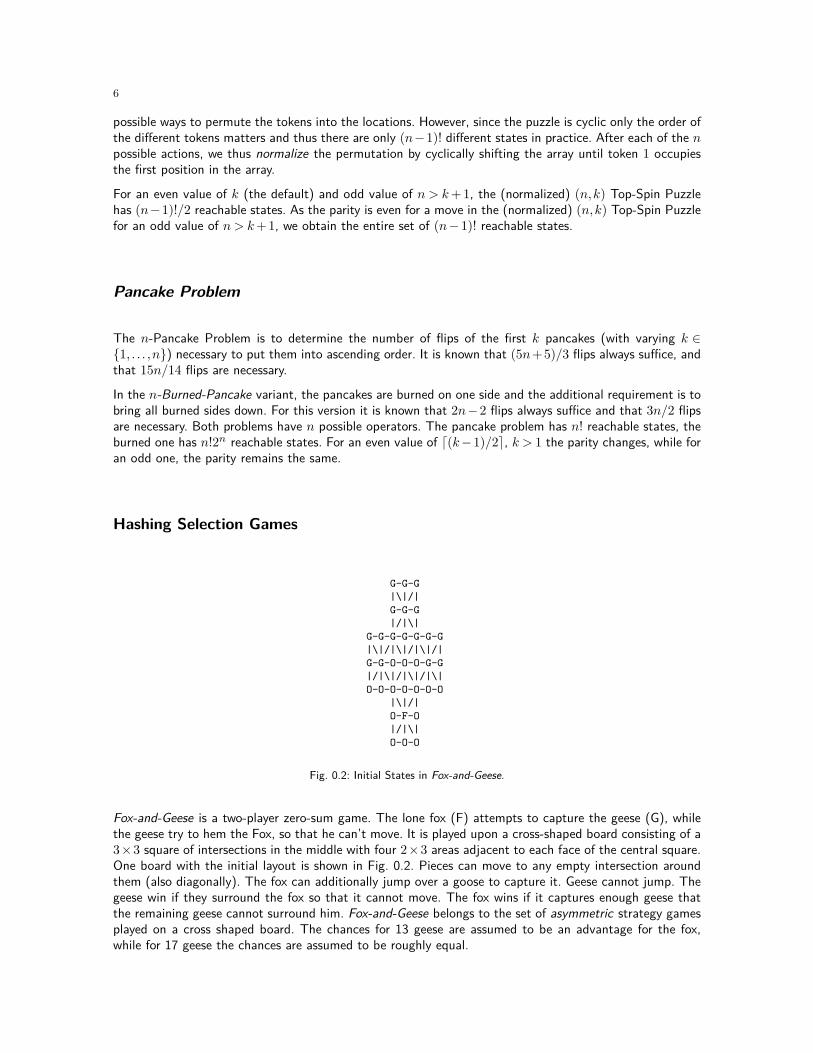
Fig. 0.2: Initial States in Fox-and-Geese.

Fox-and-Geese is a two-player zero-sum game. The lone fox (F) attempts to capture the geese (G), whilethe geese try to hem the Fox, so that he can’t move. It is played upon a cross-shaped board consisting of a3×3 square of intersections in the middle with four 2×3 areas adjacent to each face of the central square.One board with the initial layout is shown in Fig. 0.2. Pieces can move to any empty intersection aroundthem (also diagonally). The fox can additionally jump over a goose to capture it. Geese cannot jump. Thegeese win if they surround the fox so that it cannot move. The fox wins if it captures enough geese thatthe remaining geese cannot surround him. Fox-and-Geese belongs to the set of asymmetric strategy gamesplayed on a cross shaped board. The chances for 13 geese are assumed to be an advantage for the fox,while for 17 geese the chances are assumed to be roughly equal.

7

The game requires a strategic plan and tactical skills in certain battle situations. The portions of tacticand strategy are not equal for both players, such that a novice often plays better with the fox than withthe geese. A good fox detects weaknesses in the set of goose (unprotected ones, empty vertices, which arecentral to the area around) and moves actively towards them. Potential decoys, which try to lure the foxout of his burrow have to be captured early enough. The geese have to work together in form of a swarmand find a compromise between risk and safety. In the beginning it is recommended to choose safe moves,while to the end of the game it is recommended to challenge the fox to move out in order to fill blockedvertices.

O O O X X XO O O X X XO O X X -> X X O O

X X X O O OX X X O O O

Fig. 0.3: Initial and goal state in Fore and Aft.

X X X O O OX X X O O O

X X X X X X X O O O O O O OX X X O X X X -> O O O X O O OX X X X X X X O O O O O O O

X X X O O OX X X O O O

Fig. 0.4: Initial and goal state in Peg Solitaire.

The Fore and Aft puzzle (see Fig. 0.3) has been made popular by the American puzzle creator Sam Loyd.It is played on a part of the 5× 5 board consisting of two 3× 3 subarrays at diagonally opposite corners.They overlap in the central square. One square has 8 black pieces and the other has 8 white pieces, withthe centre left vacant. The objective is to reverse the positions of pieces in the lowest number of moves.Pieces can slide or jump over another pieces of any colour. Frogs-and-Toads generalizes Fore and Aft andlarge boards are yet unsolved.

In Peg-Solitaire (see Fig. 0.4) the set of pegs is iteratively reduced by jumps. The problem can be generalizedto an arbitrary graph with n holes. As the number of pegs denote the progress in playing Peg-Solitaire,we may aim at representing all boards with k of the n−1 possible pegs, where n is the number of holes.In fact, the breadth-first level k contains at most

(nk

)states. In contrast to permutation games, pegs are

indistinguishable, and call for a different design of a hash function and its inverse.

Such an inversible perfect hash function of all states that have k = 1, . . . ,n pegs remaining on the boardreduces the RAM requirements for analyzing the game. As successor generation is fast, we will need anefficient hash function (rank) that maps bitvectors (s0, . . . ,sn−1) ∈ {0,1}n with k ones to {0, . . . ,

(nk

)−1}

and back (unrank). There is a trivial ranking algorithm that uses a counter to determine the numberof bitvectors passed in their lexicographic ordering that have k ones. It uses linear space, but the timecomplexity by traversing the entire set of bitvectors is exponential. The unranking algorithm works similarlywith matching exponential time performance.

The design of a linear time ranking and unranking algorithm is not obvious. The pieces on the board arenot labeled, their relative ordering does not matter.

8

Hashing with Binomial Coefficients

An efficient solution for perfect and inversible hashing of all bitvectors with k ones to {0, . . . ,(n

k

)−1} utilize

binomial coefficients that can either be precomputed or determined on-the-fly. The algorithms rely on theobservation that once a bit at position i in a bitvector with n bits and with j zeros is processed, the binomialcoefficient

( ij−1)can be added to the rank. The notation max

{0,( izeros−1

)}is shorthand notation to say,

if zeros< 1 take 0, otherwise take( izeros−1

).

The time complexities of both algorithms are O(n). In case the number of zeros exceeds the number ofones, the rank and unrank algorithms can be extended to the inverted bitvector representation of a state.

The correctness argument relies on the binomial coefficients labeling a grid graph of nodes Bi,j with idenoting the position in the bit-vector and j denoting the number of zeros already seen. Let Bi,j beconnected via a directed edge to Bi−1,j and Bi−1,j−1 corresponding to a zero and an one processed in thebit-vector. Starting at Bi,j there are

(ij

)possible non-overlapping paths that reach B0,z. These pathcount-

values can be used to determine the index of a given bitvector in the set of all possible ones. At the currentnode (i, j) in the grid graph in case of the state at position i containing a

• 1: all path-counts at Bi−1,j−1 are added.

• 0: nothing is added.

Hashing with Multinomial Coefficients

The perfect hash functions derived for games like Peg-Solitaire are often insufficient in games with piecesof different color like TicTacToe and Nine-Men-Morris. For this case, we have to devise a hash functionthat operates on state vectors of size n that contain zeros (location not occupied), ones (location occupiedby pieces of the first player) and twos (location occupied by pieces of the second player). We will determinethe value of a position by hashing all state with a fix number of z zeros, and o ones and t= n−z−o twosto a value in {0, . . . ,

( nz,o,t

)−1}, where the multinomial coefficient

( nz,o,t

)is defined as(

n

z,o, t

)= n!z! ·o! · t! .

The correctness argument relies on representing the multinomial coefficients in a 3D grid graph of nodesBi,j,l with i denoting the index position in the vector and j denoting the number of zeros j, and l denotingthe number of ones already seen. The number of twos is then immediate. Let Bi,j,l be connected via adirected edge to Bi−1,j,l, Bi−1,j,l−1 and Bi−1,j−1,l corresponding to a value 2, 1 or 0 processed in thebit-vector, respectively. There are

( ij,l,n−j−l

)possible non-overlapping paths starting from each node Bi,j,l

that reach B0,z,o. These pathcount-values can be used to determine the index of a given bitvector in theset of all possible ones. At the current node (i, j, l) in the grid graph in case of the node at position icontaining a

• 1: all path-counts values at Bi−1,j−1,l are added.

• 2: all path-counts values at Bi−1,j,l−1 are added.

• 0: nothing is added.

9

Parallelization

Parallel processing is the future of computing. On current personal computer systems with multiple coreson the CPU and (graphics) processing units on the graphics card, parallelism is available “for the masses”.For our case of solving games, we aim at fast successor computation. Moreover, ranking and unrankingthat take substantial running time are executed in parallel.

To improve the I/O behavior, the partitioned state space was distributed over multiple hard disks. Thisincreased the reading and writing bandwidth and enabled each thread to use its own hard disk. In largerinstances that exceed RAM capacities we additionally maintain write buffers to avoid random access ondisk. Once the buffer is full, it is flushed to disk. In one streamed access, all corresponding bits are set.

Multi-Core Computation

Nowadays computers have multiple cores, which reduce the runtime of an algorithm by distributing theworkload to concurrently running threads. We use pthreads for such multi-threading support.

Let Sp be the set of all possible positions in Fox-and-Geese (Frogs-and-Toads) with p pieces, which togetherwith the fox position and the player’s turn uniquely address states in the game. During play, the numberof pieces decreases (or stays) such that we partition backward (forward) BFS layers into disjoint setsSp = Sp,0∪ . . .∪Sp,n−1. As |Sp,i| ≤

(n−1p

)is constant for all i ∈ {0, . . . ,n−1}, a possible upper bound on

the number of reachable states with p pieces is n ·(n−1

p

). These states will be classified by our algorithm.

In two-bit retrograde (bfs) analysis all layers Layer0,Layer1, . . . are processed in partition form. The fixpointiteration to determine the solvability status in one backward (forward) BFS level Layerp =Sp,0∪ . . .∪Sp,n−1is the most time consuming part. Here, we can apply a multi-core parallelization using pthreads. In total, nthreads are forked and joined after completion. They share the same hash function, and communicate fortermination.

For improving space consumption we urge the exploration to flush the sets Sp,i whenever possible and toload only the ones needed for the current computation. In the retrograde analysis of Fox-and-Geese theaccess to positions with a smaller number of pieces Sp−1 is only needed during the initialization phase. Assuch initialization is a simple scan through a level we only need one set Sp,i at a time. To save space forthe fixpoint iteration, we release the memory needed to store the previous layer. As a result, the maximumnumber of bits needed is max{|Sp|, |Sp|/n+ |Sp−1|).

GPU Computation

In the last few years there has been a remarkable increase in the performance and capabilities of thegraphics processing unit. Modern GPUs are not only powerful, but also parallel programmable processorsfeaturing high arithmetic capabilities and memory bandwidths. Deployed on current graphic cards, GPUshave outpaced CPUs in many numerical algorithms. The GPU’s rapid increase in both programmability andcapability has inspired researchers to map computationally demanding, complex problems to the GPU.

GPUs have multiple cores, but the programming and computational model are different from the ones on theCPU. Programming a GPU requires a special compiler, which translates the code to native GPU instructions.The GPU architecture mimics a single instruction multiply data (SIMD) computer with the same instructions

10

running on all processors. It supports different layers for memory access, forbids simultaneous writes butallows concurrent reads to one memory cell.

Memory, is structured hierarchically, starting with the GPU’s global memory (video RAM, or VRAM). Accessto this memory is slow, but can be accelerated through coalescing, where adjacent accesses with less than64 bits are combined to one 64-bit access. Each SM includes 16 KB of memory (SRAM), which is sharedbetween all SPs and can be accessed at the same speed as registers. Additional registers are also located ineach SM but not shared between SPs. Data has to be copied from the systems main memory to the VRAMto be accessible by the threads.

The GPU programming language links to ordinary C-sources. The function executed in parallel on the GPUis called kernel. The kernel is driven by threads, grouped together in blocks. The TSC distributes the blocksto its SMs in a way that none of them runs more than 1,024 threads and a block is not distributed amongdifferent SMs. This way, taking into account that the maximal blockSize of 512, at most 2 blocks can beexecuted by one SM on its 8 SPs. Each SM schedules 8 threads (one for each SP) to be executed in parallel,providing the code to the SPs. Since all the SPs get the same chunk of code, SPs in an else-branch wait forthe SPs in the if-branch, being idle. After the 8 threads have completed a chunk the next one is executed.Note that threads waiting for data can be parked by the SM, while the SPs work on threads, which havealready received the data.

To profit from coalescing, threads should access adjacent memory contemporary. Additionally, the SIMDlike architecture forces to avoid if-branches and to design a kernel which will be executed unchanged forall threads. This facts lead to the implementation of keeping the entire or partitioned state space bitvectorin RAM and copying an array of indices (ranks) to the GPU. This approach benefits from the SIMDtechnology but imposes additional work on the CPU. One additional scan through the bitvector is neededto convert its bits into integer ranks, but on the GPU the work to unrank, generate the successors and rankthem is identical for all threads. To avoid unnecessary memory access, the rank given to expand should beoverwritten with the rank of the first child. As the number of successors is known beforehand, with eachrank we reserve space for its successors. For smaller BFS layers this means that a smaller amount of statesis expanded.

For solving games on the graphics card, storing the bitvector on the GPU yields bad exploration results.Hence, we forward the bitvector indices from the CPU’s host RAM to the GPU’s VRAM, where they wereuploaded to the SRAM, unranked and expanded, while the successors were ranked. At the end of oneiteration, all successors are moved back to CPU’s host RAM, where they are perfectly hashed and markedif new.

Experiments Explicit-State Perfect Hashing

We start presentation of the experiments in permutation games (mostly showing the effect of multi-coreGPU computation) followed by selection games (also showing the effect of multi-core CPU computation).

For measuring the speed-up on a matching implementation we compare the GPU performance with a CPUemulation on a single core. This way, the same code and work was executed on the CPU and the GPU. Fora fair comparison, the emulation was run with GPU code adjusted to one thread. This minimizes the workfor thread communication on the CPU. Moreover, we profiled that the emulation consumed most CPU timefor state expansion and ranking.

11

Sliding-Tile Puzzle

The results of the first set of experiments shown in Table 0.1 illustrate the effect of bitvector state spacecompression with breadth-first search in rectangular Sliding-Tile problems of different sizes.

We run both the one- and two-bit breadth-first search algorithms on the CPU and GPU. The 3×3 versionwas simply too small to show significant advances, while even in partitioned form a complete explorationon a bit vector representation of the 15-Puzzle requires more RAM than available.

We first validated that all states were generated and equally distributed among the possible blank positions.Moreover, as expected, the numbers of BFS layers for symmetric puzzle instances match (53 for 3×4 and4×3 as well as 63 for 2×6 and 6×2).

For the 2-Bit BFS implementation, we observe a moderate speed-up by a factor between 2 and 3, which isdue to the fact that the BFS-layers of the instances that could be solved in RAM are too small. For suchsmall BFS layers, further data processing issues like copying the indices to the VRAM is rather expensivecompared to the gain achieved by parallel computation on the GPU. Unfortunately, the next larger instance(7× 2) was too large for the amount of RAM available in the machine (it needs 3× 750 = 2,250 MB forOpen and 2 GB for reading and writing indices to the VRAM).

In the 1-Bit BFS implementation the speed-up increases to a factor between 7 and 10 in the small instances.Many states are re-expanded in this approach, inducing more work for the GPU and exploiting its potentialfor parallel computation. Partitions being too large for the VRAM are split and processed in chunks of about250 millions indices (for the 7×2 instance). A quick calculation shows that the savings of GPU computationare large. We noticed that the GPU has the capability to generate 83 million states per second (includingunranking, generating the successors and computing their rank) compared to about 5 million states persecond of the CPU. As a result, for the CPU experiment that ran out of time (o.o.t), which we stoppedafter one day of execution, we predict a speed-up factor of at least 16, and a running time of over 60 hours.

2-Bit Time 1-Bit TimeProblem GPU CPU GPU CPU(2 × 6) 1m10s 2m56s 2m43s 15m17s(3 × 4) 55s 2m22s 1m38s 13m53s(4 × 3) 1m4s 2m22s 1m44s 12m53s(6 × 2) 1m26s 2m40s 1m29s 18m30s(7 × 2) o.o.m. o.o.m. 226m30s o.o.t.

Table 0.1: Comparing GPU with CPU performances in 1-Bit and 2-Bit BFS in sliding-tile puzzles.

Top-Spin Problems

The results for the (n,k)-Top-Spin problems for a fixed value of k= 4 are shown in Table ?? (o.o.m denotesout of memory, while o.o.t denotes out of time). We see that the experiments validate the theoreticalstatement of Theorem 1 that the state spaces are of size (n− 1)!/2 for n being odd and (n− 1)! for neven. For large values of n, we obtain a significant speed-up of more than factor 30.

12

n States GPU Time CPU Time6 120 0s 0s7 360 0s 0s8 5,040 0s 0s9 20,160 0s 0s

10 362,880 0s 6s11 1,814,400 1s 35s12 39,916,800 27s 15m20s

Table 0.2: Comparing GPU with CPU performances for Two-Bit-BFS in the Top-Spin.

n States GPU Time CPU Time9 362,880 0s 4s

10 3,628,800 2s 48s11 39,916,800 21s 10m41s12 479,001,600 6m50s 153m7s

Table 0.3: Comparing GPU with CPU performances in Two-Bit-BFS in Pancake problems.

Pancake Problems

The GPU and CPU running time results for the n-Pancake problems are shown in Table 0.3. Similar to theTop-Spin puzzle for a large value of n, we obtain a speed-up factor of more than 30 wrt. running the samealgorithm on the CPU.

Peg-Solitaire

The first set of results, shown in Table 0.4, considers Peg-Solitaire. For each BFS-layer, the state space issmall enough to fit in RAM. The exploration result show that there are 5 positions with one peg remaining(of course there is none with zero pegs), one of which has the peg in the goal position.

In Peg-Solitaire we find a symmetry, which applies to the entire state space. If we invert the board (ex-changing pegs with holes or swapping the colors), the goal and the initial state are the same. Moreover,the entire forward and backward graph structures match.

Hence, a call of backward breadth-first search to determine the number of states with a fixed goal distanceis not needed. The number of states with a certain goal distances matches the number of states with a thesame distance to the initial state. The total number of reachable states is 187,636,298.

We parallelized the game expanding and ranking states on the GPU. The total time for a BFS we measuredwas about 12m on the CPU and 1m8s on the GPU.

As the puzzle is moderately small, we consider the GPU speed-up factor of about 6 wrt. CPU computationas being significant.

The exploration results match with the ones in our general game player. For this case we had to alter thereward structure to the one that is imposed by the general game description language that was used there.We found that the number of expanded states matches, but – as expected – the total time to classify thestates using the specialized player on the GPU is much smaller than in the general player running on onecore of the CPU.

13

Holes Bits Space Expanded0 1 1 B –1 33 5 B 12 528 66 B 43 5,456 682 B 124 40,920 4,99 KB 605 237,336 28,97 KB 2966 1,107,568 135 KB 1,3387 4,272,048 521 KB 5,6488 13,884,156 1.65 MB 21,8429 38,567,100 4.59 MB 77,55910 92,561,040 11.03 MB 249,69011 193,536,720 23.07 MB 717,78812 354,817,320 42.29 MB 1,834,37913 573,166,440 68.32 MB 4,138,30214 818,809,200 97.60 MB 8,171,20815 1,037,158,320 123 MB 14,020,16616 1,166,803,110 139 MB 20,77323617 1,166,803,110 139 MB 26,482,82418 1,037,158,320 123 MB 28,994,87619 818,809,200 97.60 MB 27,286,33020 573,166,440 68.32 MB 22,106,34821 354,817,320 42.29 MB 15,425,57222 193,536,720 23.07 MB 9,274,49623 92,561,040 11.03 MB 4,792,66424 38,567,100 4.59 MB 2,120,10125 13,884,156 1.65 MB 800,15226 4,272,048 521 KB 255,54427 1,107,568 135 KB 68,23628 237,336 28.97 KB 14,72729 40,920 4.99 KB 252930 5,456 682 B 33431 528 66 B 3332 33 5 B 533 1 1 B -

Table 0.4: Applying One-Bit-BFS to Peg-Solitaire.

Frogs-and-Toads

Similar to Peg-Solitaire if we invert the board (swapping the colors of the pieces), the goal and the initialstate are the same, so that forward breadth-first search sufficies to solve the game. The result of Dudeneyfor Fore and Aft that reversing black and white takes 46 moves are easily validated with BFS. There aretwo positions which require 47 moves, namely, after reversing black and white, putting one of the far cornerpieces in the center. Table 0.5 also shows that there are 218,790 position in total.

As Frogs-and-Toads generalizes Fore and Aft, we next considered the variant with 15 black and 15 whitepieces on a board with 31 squares. The BFS outcome is shown in Table 0.6. We monitored that reversingblack and white pieces takes 115 steps (in a shortest solution) and see that the worst-case input is slightlyharder and takes 117 steps. A GPU parallelization leading to the same exploration results required abouthalf an hour run-time.

14

Depth Expanded1 12 83 134 145 326 587 1218 1789 28410 49411 79412 1,143

Depth Expanded13 1,70014 2,38615 3,22316 4,24217 5,67718 7,33019 8,72220 10,08421 11,50122 12,87923 13,99724 14,804

Depth Expanded25 15,43326 14,98127 14,01528 12,84829 11,66630 10,43931 9,33432 7,85833 6,07534 4,65135 3,45936 2,682

Depth Expanded37 1,99038 1,40139 91440 55741 34842 20243 13744 6645 3246 447 1148 2

Table 0.5: BFS Results for Fore and Aft.

Depth Expanded1 12 83 174 265 466 787 1698 3189 55210 97411 1,72012 2,90513 4,82614 7,87815 12,64716 19,98017 31,51118 49,24219 74,76020 112,21821 166,65122 241,15723 348,88624 497,69825 700,06026 974,21927 1,337,48028 1,812,71229 2,426,76930 3,214,074

Depth Expanded31 4,199,88632 5,447,66033 6,975,08734 8,865,64835 11,138,98636 13,881,44937 17,060,94838 20,800,34739 25,048,65240 29,915,08241 35,382,94242 41,507,23343 48,277,76744 55,681,85345 63,649,96946 72,098,32747 80,937,54748 89,999,61349 99,231,45650 108,495,90451 117,679,22952 126,722,19053 135,363,89454 143,534,54655 150,897,87856 157,334,08857 162,600,93358 166,634,14859 169,360,93960 170,829,205

Depth Expanded61 171,101,87462 170,182,83763 168,060,81664 164,733,84565 160,093,74666 154,297,24767 147,342,82568 139,568,85569 131,146,07770 122,370,44371 113,415,29472 104,380,74873 95,379,85074 86,375,53575 77,534,24876 68,891,43977 60,672,89778 52,953,46379 45,889,79880 39,482,73781 33,751,89682 28,607,39583 24,035,84484 19,957,39285 16,394,45386 13,306,65987 10,695,28488 8,521,30489 6,738,55790 5,286,222

Depth Expanded91 4,109,15792 3,156,28893 2,387,87394 1,780,52195 1,307,31296 948,30097 680,29998 484,20799 340,311100 235,996101 160,153102 107,024103 69,216104 44,547105 27,873106 17,394107 10,256108 6,219109 3,524110 2,033111 1,040112 532113 251114 154115 42116 19117 10118 2

Table 0.6: BFS Results for Frogs-and-Touds.

Fox-and-Geese

The next set of results shown in Table 0.7 considers the Fox-and-Geese game, where we applied retrogradeanalysis. For a fixed fox position the remaining geese can be binomially hashed. Moves stay in the samepartition. It is possible to complete the analysis with 12 GB RAM. The largest problem with 16 geeserequired 9.2 GB RAM.)

15

The first three levels do not contain any state won for the geese, which matches the fact that four geeseare necessary to block the fox (at the middle boarder cell in each arm of the cross). We observe that aftera while, the number of iterations shrinks for a raising number of geese. This matches the experience thatwith more geeses it is easier to block the fox.

Recall that all potentially drawn positions that couldn’t been proven won or lost by the geese, are devisedto be a win for the fox. The critical point, where the fox looses more than 50% of the game seems to bereached at currently explored level 16. This matches the observation in practical play, that the 13 geese aretoo less to show an edge for the geese.

The total run-time of about a month for the experiment is considerable. Without multi-core parallelization,however, more than 7 month would have been needed to complete the experiments. Even though weparallized only the iteration stage of the algorithm, the speed-up on the 4-core hyper-threaded machine islarger than 7, showing an almost linear speed-up.

The total of space needed for operating an optimal player is about 34 GB, so that in case geese are capturedwe would have to reload data from disk. This strategy yields a maximal space requirement of 4.61 GB RAM,which might further be reduced by reloading data in case of a fox moves.

Geese States Space Iterations Won Time Real Time User1 2,112 264 B 1 0 0.05s 0.08s2 32,736 3.99 KB 6 0 0.55s 1.16s3 327,360 39 KB 8 0 0.75s 2.99s4 2,373,360 289 KB 11 40 6.73s 40.40s5 13,290,816 1.58 MB 15 1,280 52.20s 6m24s6 59,808,675 7.12 MB 17 21,380 4m37s 34m40s7 222,146,996 26 MB 31 918,195 27m43s 208m19s8 694,207,800 82 MB 32 6,381,436 99m45s 757m0s9 1,851,200,800 220 MB 31 32,298,253 273m56s 2,083m20s10 4,257,807,840 507 MB 46 130,237,402 1,006m52s 7,766m19s11 8,515,615,680 1015 MB 137 633,387,266 5,933m13s 46,759m33s12 14,902,327,440 1.73 GB 102 6,828,165,879 4,996m36s 36,375m09s13 22,926,657,600 2.66 GB 89 10,069,015,679 5,400m13s 41,803m44s14 31,114,749,600 3.62 GB 78 14,843,934,148 5,899m14s 45,426m42s15 37,337,699,520 4.24 GB 73 18,301,131,418 5,749m6s 44,038m48s16 39,671,305,740 4.61 GB 64 20,022,660,514 4,903m31s 37,394m1s17 37,337,699,520 4.24 GB 57 19,475,378,171 3,833m26s 29,101m2s18 31,114,749,600 3.62 GB 50 16,808,655,989 2,661m51s 20,098m3s19 22,926,657,600 2.66 GB 45 12,885,372,114 1,621m41s 12,134m4s20 14,902,327,440 1.73 GB 41 8,693,422,489 858m28s 6,342m50s21 8,515,615,680 1015 MB 5,169,727,685 395m30s 2,889m45s22 4,257,807,840 507 MB 31 2,695,418,693 158m41s 1,140m33s23 1,851,200,800 220 MB 26 1,222,085,051 54m57 385m32s24 694,207,800 82 MB 23 477,731,423 16m29s 112m.35s25 222,146,996 26 MB 20 159,025,879 4m18s 28m42s26 59,808,675 7.12 MB 17 44,865,396 55s 5m49s27 13,290,816 1.58 MB 15 10,426,148 9.81s 56.15s28 2,373,360 289 KB 12 1,948,134 1.59s 6.98s29 327,360 39 KB 9 281,800 0.30s 0.55s30 32,736 3.99 KB 6 28,347 0.02s 0.08s31 2,112 264 B 5 2001 0.00s 0.06s

Table 0.7: Retrograde analysis results for Fox-and-Geese.

16

Symmetries, Frontier Search, and Generality

In many board games we find symmetries like reflection along the main axes or along the diagonals. Ifwe look at the four possible rotations on the board for Peg-Solitaire and Fox-and-Geese plus reflection,we count 8 symmetries in total. For Fox-and-Geese we can classify all states that share a symmetrical foxposition by simply copying the result obtained for the existing one. Besides the savings of time for notexpanding states, this can also save the number of positions that have to be kept in RAM during fixpointcomputation. If the forward and backward search graphs match (as in Peg Solitaire and Frogs-and-Toads)we may also truncate the breadth-first search proceedure to the half of the search depth. In two-bit BFS,we simply have to look at the rank of the inverted unranked state. Moreover, with the forward BFS layerswe also have the minimal distances of each state to the goal state, and, hence, the classification result.

Frontier search is motivated by the attempt of omitting the Closed list of states already expanded. Itmainly applies to problem graphs that are directed or acyclic but has been extended to more general graphclasses. It is especially effective if the ratio of Closed to Open list sizes is large. Frontier search requiresthe locality of the search space being bounded, where the locality (for breadth-first search) is defined asmax{layer(s)− layer(s′)+1 | s,s′ ∈S;s′ ∈ succs(s)}, where layer(s) denotes the depth d of s in the breadth-first search tree. For frontier search, the space efficiency of the hash function h : S→ {0, . . . ,m−1} boilsdown to m/

(maxd |Layerd|+ . . .+ |Layerd+l|

), where Layerd is set of nodes in depth d of the breadth-first

search tree and l is the locality of the breadth-first search tree as defined above.

For the example of the Fifteen puzzle, i.e., the 4× 4 version of Sliding-Tile, the predicted amount of 1.2TB hard disk space for 1-bit breadth-first search is only slightly smaller than the 1.4 TB of frontier breadth-first search. As frontier search does not shrink the set of states reachable, one may conclude, that frontiersearch hardly cooperates well with a bitvector representation of the entire state space. However, if layersare hashed individually, as done in all selection games we have considered, a combination of bit-state andfrontier search is possible.

Compressed Pattern Databases

The number of bits per state can be reduced to log3≈ 1.6. For this case, 5 values {0,1,2} are packed intoa byte, given that 35 = 243< 255.

The idea of pattern database compression is to store the mod-3 value (of the backward BFS depth)from abstract space, so that its absolute value can be computed incrementally in constant time. For theinitial state, an incremental computation for its heuristic evaluation is not available, so that a backwardconstruction of its generating path can be used. For an undirected graph a shortest path predecessor withmod-3 of BFS depth k appears in level k−1 mod 3.

As the abstract space is generated anyway for generating the database, one could alternatively invoke ashortest path search from the initial state, without exceeding the time complexity of database construction.

By having computed the heuristic value for the projected initial state as the goal distance in the invertedabstract state space graph, all other pattern database lookup values can then be determined incrementally inconstant time, i.e., h(v) = h(u)+∆(v), with v ∈ succs(u) and ∆(v) found using the mod-3 value of v. If theconsidered search spaces are undirected, the information to evaluate the successors with ∆(v) ∈ {−1,0,1}is possible.

For directed (and unweighted) search spaces more bits are needed to allow incremental heuristic computationin constant time. It is not difficult to see that the locality in the inverted abstract state space determinesthe maximum difference in h-values h(v)−h(u), v ∈ succs(u) in original space.

Theorem 0.1 (Locality determines Pattern Database Compression). In a directed (but unweighted)search space, the (dual) logarithm of the (breadth-first) locality of the inverse of the abstract state space

17

graph plus 1 is an upper bound on the number of bits needed for incremental heuristic computation ofbit-vector compressed pattern databases, i.e., for locality l−1

A = max{layer−1(u)− layer−1(v) + 1 | u,v ∈A;v ∈ succs−1(u)} in abstract state space graph A of S we require at most logdl−1

A e+1 bits to reconstructthe value h(v) of a successor v ∈ S of any chosen u ∈ S given h(u).

Proof. First we observe that the goal distances in abstract space A determine the h-value in originalstate space, so that the locality max{layer−1(u)− layer−1(v) + 1 | u,v ∈ A;v ∈ succs−1(u)} is boundedby h(u)−h(v) + 1 for all u,v in original space with u ∈ succs(v), which is equal to the maximum ofh(v)−h(u) + 1 for u,v ∈ S with v ∈ succs(u). Therefore, the number of bits needed for incrementalheuristic computation equals dmax{h(v)− h(u) | u,v ∈ A;v ∈ succs−1(u)}e+ 2 as all values in theinterval [h(u)−1, . . . ,h(v)] have to be accomodated for. Thus for the incremental value ∆(v) added toh(u) we have ∆(v)∈ {−1, . . . ,h(v)−h(u)}, so that dlog(max{h(v)−h(u)+2 | u,v ∈ S;v ∈ succs(u)})e=logdl−1

A e+1 bits suffice to reconstruct the value h(v) of a successor v ∈ S for every u ∈ S given h(u).

For undirected search spaces we have log l−1A = log2 = 1, so that 1 + 1 = 2 bits suffice to be stored for

each abstract pattern state according to the theorem. Using the tighter packing of the 2+1 = 3 values intobytes provided above, 8/5 = 1.6 bits are sufficent.

If not all states in the search space that has been encoded in the perfect hash function are reachable, reducingthe constant-bit compression to a lesser number of bits might not always be available, as unreached statescannot easily be removed. For this case, the numerical value remaining to be set for an unreachable statesin the inverse of abstract state space will stand for h-value infinitiy, at which the search in the originalsearch space can stop.

More formally, the best-first locality has been defined as max{cost-layer(s)− cost-layer(s′) + cost(s,s′) |s,s′ ∈ S;s′ ∈ succs(s)}, where cost-layer(s) denotes the smallest accumulated cost-value from the initialstate to s. The theoretical considerations on the number of bits needed to perform incremental heuristicevaluation extend to this setting.

Other Games

In Rubik’s Cube each face can be rotated by 90, 180, or 270 degrees and the goal is to rearrange a scrambledcube such that all faces are uniformly colored.

Solvability invariants for the set of all dissembled cubes are:

• a single corner cube must not be twisted

• a single edge cube must not be twisted and

• no two cube must be exchanged

For the last issue the parity of the permutation is crucial and leads to 8! ·37 ·12! ·211/2≈ 4.3 ·1019 solvablestates. Assuming one bit per state, an impractical amount of 4.68 ·1018 bytes for performing full reachabilityis needed.

The binomial and multinomial hashing approach is applicable to many other pen-and-paper and boardgames.

• In Awari the two player redistribute seeds among 12 holes according to the rules of the game, with aninitial state having uniformly four seeds in each of the holes. When all seeds are available, all possiblelayouts can be genrated in an urn experiments with 59 balls, where 48 balls represent filling the currenthole with a seed and 11 balls indicate changing from the current to the next hole. Thus the binomialhash function applies.

18

• In Dots and Boxes players take turns joining two horizontally or vertically adjacent dots by a line. Aplayer that completes the fourth side of a square (a box) colors that box and must play again. Whenall boxes have been colored, the game ends and the player who has colored more boxes wins. Here, thebinomial hash suffices. For each edge we denote whether or not it is marked. Together with the marking,we denote the number of boxes of at least one player. In difference to other games, all successors are inthe next layer, so that one scan suffices to solve the current one.

• Nine-Men’s-Morris is one of the oldest games still played today. The game naturally divides in threestages. Each player has 9 pieces, called men, that are first placed alternately on a board with 24 locations.In the second stage, the men move to form mills (a row of three pieces along one of the board’s lines),in which case one man of the opponent (except the ones that form a mill) is removed from the board.In one common variation of the third stage, once a player is reduced to three men, his pieces may “fly”to any empty location. If a move has just closed a mill, but all the opponent’s men are also in mills, theplayer may declare any stone to be removed. The game ends if a player has less than three men (theplayer loses), if a player cannot make a legal move (the player loses), if a midgame or endgame positionis repeated (the game is a draw).

Besides the usual symmetries along the axes, there is one in swapping the inner with the outer circle.For this game the multinomial hash is applicable.

Binary Decision Diagrams for Strongly Solving Games

In general state spaces minimum perfect hash functions with a few bits per state can be constructed (I/O-efficiently) after generating the state space (on disk). This requires c bit RAM per state (typically, c≈ 2). Ofcourse, perfect hash functions do not have to be minimal to be space-efficient. Non-minimal hash functionscan outperform minimal ones, since the gain in the constant c for the hash function can be more important,than the loss in coverage.

Binary decision diagrams (BDDs) are a memory-efficient data structure used to represent Boolean functions.A BDD is a directed acyclic graph with one root and two terminal nodes, the 0- and the 1-sink. Each internalnode corresponds to a binary variable and has two successors, one (along the Then-edge) representing thatthe current variable is true (1) and the other (along the Else-edge) representing that it is false (0). For anyassignment of the variables derived from a path from the root to the 1-sink the represented function willbe evaluated to 1.

For a fixed variable ordering, two reduction rules can be applied: eliminating nodes with the same Then andElse successors and merging two nodes representing the same variable that share the same Then successoras well as the same Else successor. These BDDs are called reduced ordered binary decision diagrams(ROBDDs). Whenever we mention BDDs in this paper, we actually refer to ROBDDs. We also assume thatthe variable ordering is the same for all the BDDs and has been optimized prior to the search.

We are interested in the image of a state set S with respect to a transition relation Trans. The result isa characteristic function of all states reachable from the states in S in one step. For the application ofthe image operator we need two sets of variables, one, x, representing the current state variables, another,x′, representing the successor state variables. The image Succ of the state set S is then computed asSucc(x′) = ∃x (Trans(x,x′) ∧ S(x)). The preimage Pre of the state set S is computed as Pre(x) =∃x′ (Trans(x,x′) ∧ S(x′)) and results in the set of predecessor states.

Using the image operator, implementing a layered symbolic breadth-first search (BFS) is straight-forward.All we need to do is to apply the image operator to the initial state resulting in the first layer, then applythe image operator to the first layer resulting in the second and so on. The search ends when no successorstates can be found. General games (and in this case, Connect Four) are guaranteed to terminate after afinite number of steps, so that the forward search will eventually terminate as well.

19

rank(s)i = level(root);d = bin(s[0..i-1]);return d*sc(root) + rankAux(root,s) - 1;

rankAux(n, s)if (n <= 1) return n;i = level(n);j = level(Else(n));k = level(Then(n));if (s[i] == 0)

return bin(s[i+1..j-1]) * sc(Else(n))+ rankAux(Else(n),s);

elsereturn 2^(j-i-1) * sc(Else(n))

+ bin(s[i+1..k-1]) * sc(Then(n))+ rankAux(Then(n),s);

unrank(r)i = level(root);d = r / sc(root);s[0..i-1] = invbin(d);n = root;while (n > 1)

r = r mod sc(n);j = level(Else(n));k = level(Then(n));if (r < (2^(j-i-1) * sc(Else(n))))

s[i] = 0;d = r / sc(Else(n));s[i+1..j-1] = invbin(d);n = Else(n);i = j;

elses[i] = 1;r = r - (2^(j-i-1) * sc(Else(n)));d = r / sc(Then(n));s[i+1..k-1] = invbin(d);n = Then(n);i = k;

return s;

Fig. 0.5: Ranking and unranking.

The problem of the construction og perfect hash functions for algorithms like two-bit breadth-first searchis that most of them are problem-dependent. Hence, for the construction of the perfect hash function, theunderlying state set to be hashed is generated in advance in form of a BDD. This is true, when computingstrong solutions to problems, where we are interested in the game-theoretical value of all reachable states.Applications are, e.g., endgame databases or planning tasks where the problem to be solved is harder thancomputing the reachability set.

The index(n) of a BDD node n is its unique position in the shared representation and level(n) its positionin the variable ordering. Moreover, we assume the 1-sink to have index 1 and the 0-sink to have index 0.Let Cf = |{a ∈ {0,1}n | f(a) = 1}| denote the number of satisfying assignments (satcount, here also scfor short) of f . With bin (and invbin) we denote the conversion of the binary value of a bitvector (and itsinverse). The rank of a satisfying assignment a ∈ {0,1}n is the position in the lexicographical ordering ofall satisfying assignments, while the unranking of a number r in {0, . . . ,Cf −1} is its inverse.

Fig. 0.5 shows the ranking and unranking functions in pseudo-code. The procedures determine the rankgiven a satisfying assignment and vice versa. They access the satcount values on the Else-successor of eachnode (adding for the ranking and subtracting in the unranking). Missing nodes (due to BDD reduction)have to be accounted for by their binary representation, i.e., gaps of l missing nodes are accounted for 2l.While the ranking procedure is recursive the unranking procedure is not.

The satcount values of all BDD nodes are precomputed and stored along with the nodes. As BDDs arereduced, not all variables on a path are present but need to be accounted for in the satcount procedure.The time (and space) complexity of it is O(|Gf |), where |Gf | is the number of nodes of the BDD Gf

representing f . With the precomputed values, rank and unrank both require linear time O(n), where n isthe number of variables in the function represented in the BDD.

To illustrate the ranking and unranking procedures, take the example BDD given in Figure 0.6. Assume wewant to calculate the rank of state s= 110011. The rank of s is then

20

rank(s) = 0+ rA(v13,s)−1 = (21−0−1 ·sc(v11)+0+ rA(v16,s))−1= sc(v11)+(23−1−1 ·sc(v8)+ bin(0) ·sc(v9)+ rA(v9,s))−1= sc(v11)+2sc(v8)+(0+ rA(v5,s))−1= sc(v11)+2sc(v8)+(26−4−1 ·sc(v0)+ bin(1) ·sc(v1)+ rA(v1,s))−1= sc(v11)+2sc(v8)+2sc(v0)+sc(v1)+1−1= 14+2 ·5+2 ·0+1+1−1 = 25

with rA(s,vi) being the recursive call of the rankAux function for state s in node vi and sc(vi) the satcountstored in node vi.

0 1

30

14 16

4

2 2 5 3

1 1 2

1

v11 v12

v10

v6 v7 v8 v9

v3 v4 v5

v2

v0 v1

v13

Fig. 0.6: BDD for the ranking and unranking examples. Dashed arrows denote Else-edges; solid ones Then-edges. Thenumbers in the nodes correspond to the satcount. Each vi denotes the index (i) of the corresponding node.

For unranking the state with index 19 (r = 19) from the BDD depicted in Figure 0.6 we get:

• i = 0,n = v13: r = 19 mod sc(v13) = 19 mod 30 = 19 6< 21−0−1sc(v11) = 14, thus s[0] = 1; r = r−21−0−1sc(v11) = 19−14 = 5

• i = 1,n = v12: r = 5 mod sc(v12) = 5 mod 16 = 5 < 23−1−1sc(v8) = 2 ·5 = 10, thus s[1] = 0; s[2] =invbin(r/sc(v8)) = invbin(5/5) = 1

• i= 3,n= v8: r = 5 mod sc(v8) = 5 mod 5 = 0< 24−3−1sc(v4) = 1, thus s[3] = 0

• i= 4,n= v4: r= 0 mod sc(v4) = 0 mod 1 = 0 6< 26−4−1sc(v0) = 0, thus s[4] = 1; r= r−26−4−1sc(v0) =0−0 = 0

• i= 5,n= v2: r= 0 mod sc(v2) = 0 mod 1 = 0 6< 27−6−1sc(v12) = 0, thus s[5] = 1; r= r−27−6−1sc(v12) =0−0

• i= 6;n= v1: return s (= 101011)

Retrograde Analysis on a Bitvector

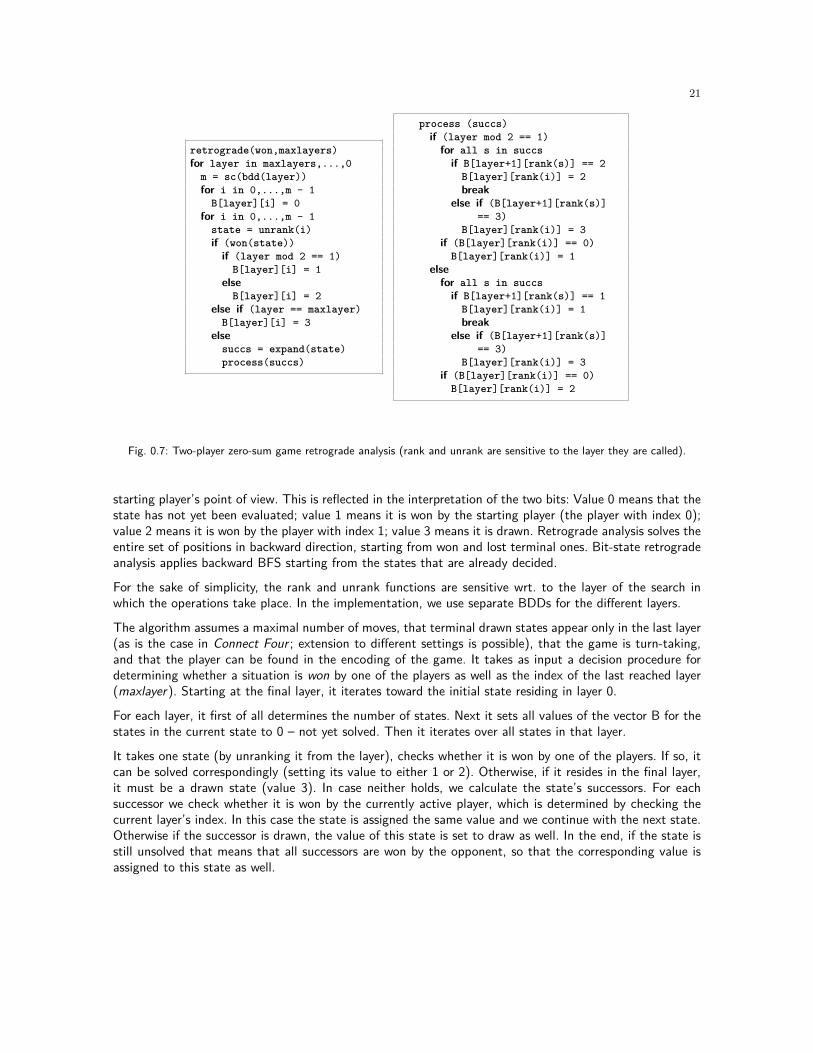
In our implementation (see Algorithm 0.7) we also use two bits, but with a different meaning. We applythe algorithm to solve two-player zero-sum games where the outcomes are only won/lost/drawn from the

21

retrograde(won,maxlayers)for layer in maxlayers,...,0

m = sc(bdd(layer))for i in 0,...,m - 1

B[layer][i] = 0for i in 0,...,m - 1

state = unrank(i)if (won(state))

if (layer mod 2 == 1)B[layer][i] = 1

elseB[layer][i] = 2

else if (layer == maxlayer)B[layer][i] = 3

elsesuccs = expand(state)process(succs)

process (succs)if (layer mod 2 == 1)

for all s in succsif B[layer+1][rank(s)] == 2

B[layer][rank(i)] = 2break

else if (B[layer+1][rank(s)]== 3)

B[layer][rank(i)] = 3if (B[layer][rank(i)] == 0)

B[layer][rank(i)] = 1else

for all s in succsif B[layer+1][rank(s)] == 1

B[layer][rank(i)] = 1break

else if (B[layer+1][rank(s)]== 3)

B[layer][rank(i)] = 3if (B[layer][rank(i)] == 0)

B[layer][rank(i)] = 2

Fig. 0.7: Two-player zero-sum game retrograde analysis (rank and unrank are sensitive to the layer they are called).

starting player’s point of view. This is reflected in the interpretation of the two bits: Value 0 means that thestate has not yet been evaluated; value 1 means it is won by the starting player (the player with index 0);value 2 means it is won by the player with index 1; value 3 means it is drawn. Retrograde analysis solves theentire set of positions in backward direction, starting from won and lost terminal ones. Bit-state retrogradeanalysis applies backward BFS starting from the states that are already decided.

For the sake of simplicity, the rank and unrank functions are sensitive wrt. to the layer of the search inwhich the operations take place. In the implementation, we use separate BDDs for the different layers.

The algorithm assumes a maximal number of moves, that terminal drawn states appear only in the last layer(as is the case in Connect Four ; extension to different settings is possible), that the game is turn-taking,and that the player can be found in the encoding of the game. It takes as input a decision procedure fordetermining whether a situation is won by one of the players as well as the index of the last reached layer(maxlayer). Starting at the final layer, it iterates toward the initial state residing in layer 0.

For each layer, it first of all determines the number of states. Next it sets all values of the vector B for thestates in the current state to 0 – not yet solved. Then it iterates over all states in that layer.

It takes one state (by unranking it from the layer), checks whether it is won by one of the players. If so, itcan be solved correspondingly (setting its value to either 1 or 2). Otherwise, if it resides in the final layer,it must be a drawn state (value 3). In case neither holds, we calculate the state’s successors. For eachsuccessor we check whether it is won by the currently active player, which is determined by checking thecurrent layer’s index. In this case the state is assigned the same value and we continue with the next state.Otherwise if the successor is drawn, the value of this state is set to draw as well. In the end, if the state isstill unsolved that means that all successors are won by the opponent, so that the corresponding value isassigned to this state as well.

22

Fig. 0.8: Hybrid algorithm: visualization of data flow in the strong solution process (left). Processing a layer in the retrogradeanalysis (right).

Hybrid Classification Algorithm

The hybrid classification algorithm combines the two precursing approaches. It generates the state spacewith symbolic forward search on disk and subsequently applies explicit-state retrograde analysis based onthe results in form of the BDD encoded layers read from disk. Fig. 0.8 illustrates the strong solution process.On the right hand side we see the bitvector used in retrograde analysis and on the left hand side we seethe BDD generated in forward search and used in backward search.

The process of solving one layer is depicted in Fig. 0.8 (right). While the bitvector in the layer n (shownat the bottom of the figure) is scanned and states within the layer are unranked and expanded, existinginformation on the solvability status of ranked successor states in the subsequent layer n+1 is retrieved.

Ranking and unranking wrt. the BDD is executed to look up the status (won/lost/drawn) of a node in theset of successors. We observed that there is a trade-off for evaluating immediate termination. There aretwo options, one is procedural by evaluating the goal condition directly on the explicit state, the other is adictionary lookup by traversing the corresponding reward BDD. In our case of Connect Four the latter wasnot only more general but also faster. A third option would be to determine if there are any successors andset the rewards according to the current layer (as it is done in the pseudo-code).

To increase the exploration performance of the system we distributed the explicit-state solving algorithmson multiple CPU cores. We divide the bitvector for the layer to be solved into equally-sized chunks. Thebitvector for the next layer is shared among all the threads.

For the ease of implementation, we duplicate the query BDDs for each individual core. This is unfortunate,as we only use concurrent read in the BDD for evaluating the perfect hash function but the computation ofthe rank involves setting and reading local variables and requires significant changes in the BDD packageto be organized lock-free.

Experiments BDD Hashing

Although most of the algorithms are applicable to most two-player games, our focus is on one particularcase, namely the game Connect Four (see Fig. 0.9). The game is played on a grid of c columns and r

23

rows. In the classical setting we have c= 7 and r = 6. While the game is simple to follow and play, it canbe rather challenging to win. This game is similar to Tic-Tac-Toe, with two main differences: The playersmust connect four of their pieces (horizontally, vertically, or diagonally) in order to win and gravity pullsthe pieces always as far to the bottom of the chosen column as possible. The number of states for differentsettings of c× r is shown in Table 0.8.

Table 0.8: Number of reachable states for Connect Four.

Layer 7 × 6 6 × 6 6 × 5 5 × 6 5 × 50 1 1 1 1 11 7 6 6 5 52 49 36 36 25 253 238 156 156 95 954 1,120 651 651 345 3455 4,263 2,256 2,256 1,075 1,0756 16,422 7,876 7,870 3,355 3,3507 54,859 24,330 24,120 9,495 9,3558 184,275 74,922 72,312 26,480 25,0609 558,186 211,042 194,122 68,602 60,842

10 1,662,623 576,266 502,058 169,107 139,63211 4,568,683 1,468,114 1,202,338 394,032 299,76412 12,236,101 3,596,076 2,734,506 866,916 596,13613 30,929,111 8,394,784 5,868,640 1,836,560 1,128,40814 75,437,595 18,629,174 11,812,224 3,620,237 1,948,95615 176,541,259 39,979,044 22,771,514 6,955,925 3,231,34116 394,591,391 80,684,814 40,496,484 12,286,909 4,769,83717 858,218,743 159,433,890 69,753,028 21,344,079 6,789,89018 1,763,883,894 292,803,624 108,862,608 33,562,334 8,396,34519 3,568,259,802 531,045,746 165,943,600 51,966,652 9,955,53020 6,746,155,945 884,124,974 224,098,249 71,726,433 9,812,92521 12,673,345,045 1,463,364,020 296,344,032 97,556,959 9,020,54322 22,010,823,988 2,196,180,492 338,749,998 116,176,690 6,632,48023 38,263,228,189 3,286,589,804 378,092,536 134,736,003 4,345,91324 60,830,813,459 4,398,259,442 352,607,428 132,834,750 2,011,59825 97,266,114,959 5,862,955,926 314,710,752 124,251,351 584,24926 140,728,569,039 6,891,603,916 224,395,452 97,021,80127 205,289,508,055 8,034,014,154 149,076,078 70,647,08828 268,057,611,944 8,106,160,185 74,046,977 40,708,77029 352,626,845,666 7,994,700,764 30,162,078 19,932,89630 410,378,505,447 6,636,410,522 6,440,532 5,629,46731 479,206,477,733 5,261,162,53832 488,906,447,183 3,435,759,94233 496,636,890,702 2,095,299,73234 433,471,730,336 998,252,49235 370,947,887,723 401,230,35436 266,313,901,222 90,026,72037 183,615,682,38138 104,004,465,34939 55,156,010,77340 22,695,896,49541 7,811,825,93842 1,459,332,899Σ 4,531,985,219,092 69,212,342,175 2,818,972,642 1,044,334,437 69,763,700

Table 0.9 displays the exploration results of the search. The set of all 4,531,985,219,092 reachable statescan be found within a few hours of computation, while explicit-state search took about 10,000 hours.

As illustrated in Table 0.10, of the 4,531,985,219,092 reachable states only 1,211,380,164,911 (about26.72%) have been left unsolved in the layered BDD retrograde analysis. (More precisely, there are

24

Fig. 0.9: The game Connect Four : the player with the gray pieces has won.

Table 0.9: Number of Nnodes and states in (7 × 6) Connect Four (l layer, n BDD nodes, s states).

l n s0 85 11 163 72 316 493 513 2384 890 1,1205 1,502 4,2636 2,390 16,4227 4,022 54,8598 7,231 184,2759 12,300 558,186

10 21,304 1,662,62311 36,285 4,568,68312 56,360 12,236,10113 98,509 30,929,11114 155,224 75,437,59515 299,618 176,541,25916 477,658 394,591,39117 909,552 858,218,74318 1,411,969 1,763,883,89419 2,579,276 3,568,259,80220 3,819,845 6,746,155,94521 6,484,038 12,673,345,045

l n s22 9,021,770 22,010,823,98823 14,147,195 38,263,228,18924 18,419,345 60,830,813,45925 26,752,487 97,266,114,95926 32,470,229 140,728,569,03927 43,735,234 205,289,508,05528 49,881,463 268,057,611,94429 62,630,776 352,626,845,66630 67,227,899 410,378,505,44731 78,552,207 479,206,477,73332 78,855,269 488,906,447,18333 86,113,718 496,636,890,70234 81,020,323 433,471,730,33635 81,731,891 370,947,887,72336 70,932,427 266,313,901,22237 64,284,620 183,615,682,38138 49,500,513 104,004,465,34939 38,777,133 55,156,010,77340 24,442,147 22,695,896,49541 13,880,474 7,811,825,93842 4,839,221 1,459,332,899

Total 4,531,985,219,092

1,265,297,048,241 states left unsolved by the algorithm, but the remaining set of 53,916,883,330 states inlayer 30 is implied by the solvability status of the other states in the layer.)

Even while providing space in form of 192GB of RAM, however, it was not possible to proceed the symbolicsolving algorithm to layers smaller than 30. The reason is while the peak of the solution for the state setshas already been passed, the BDDs for representing the state sets are still growing.

This motivates looking at other options for memory-limited search and a hybrid approach that takes thesymbolic information into account to eventually perform the complete solution of the problem.

Bibliographic Notes

Chess [10], Checkers [29] have shown competitiveness with human play. Pattern databases go back to [13]with locality been studied by [32]. More general notions of locality have been developed by [21].

One early attempt to apply state space search on GPUs was made in the context of model checking [18, 4].large-scale disk-based search has moved complex numerical operations to the graphic card [18]. As delayedelimination of duplicates is a performance bottleneck, parallel processing on the GPU was needed to improve

25

Table 0.10: Result of symbolic retrograde analysis (excl. terminal goals, l layer, n BDD nodes, s states).

l n (won) s (won) n (draw) s (draw) n (lost) s (lost)...

......

......

......

29 o.o.m. o.o.m. o.o.m. o.o.m. o.o.m. o.o.m.30 589,818,676 199,698,237,436 442,186,667 6,071,049,190 o.o.m. o.o.m.31 458,334,850 64,575,211,590 391,835,510 7,481,813,611 600,184,350 201,906,000,78632 434,712,475 221,858,140,210 329,128,230 9,048,082,187 431,635,078 57,701,213,06433 296,171,698 59,055,227,990 265,790,497 10,381,952,902 407,772,871 194,705,107,37834 269,914,837 180,530,409,295 204,879,421 11,668,229,290 255,030,652 45,845,152,95235 158,392,456 37,941,816,854 151,396,255 12,225,240,861 231,007,885 132,714,989,36136 140,866,642 98,839,977,654 106,870,288 12,431,825,174 121,562,152 24,027,994,34437 68,384,931 14,174,513,115 72,503,659 11,509,102,126 105,342,224 57,747,247,78238 58,428,179 32,161,409,500 44,463,367 10,220,085,105 42,722,598 6,906,069,44339 19,660,468 2,395,524,395 27,201,091 7,792,641,079 35,022,531 13,697,133,73740 17,499,402 4,831,822,472 13,858,002 5,153,271,363 8,233,719 738,628,81841 0 0 5,994,843 2,496,557,393 7,059,429 1,033,139,76342 0 0 0 0 0 0

sorting significantly. Since existing GPU sorting schemes did not show speedups on state vectors, refinedGPU-based Bucketsort applies. In [4] algorithms for parallel probabilistic model checking on GPUs wereproposed, exploiting the fact that probabilistic model checking relies on matrix vector multiplication. Sincethis kind of linear algebraic operations are implemented very efficiently on GPUs, these algorithms achieveconsiderable runtime improvements compared to their counterparts on standard architectures.

Cooperman and Finkelstein [12] have shown that two bits per state are sufficient to perform a breadth-firstexploration of the search space. Efficient lexicographic ranking methods are studied in [3]. Many attempts,e.g. have a non-linear worst-case time complexity [25], and [24] employed lookup tables with a spacerequirement of O(2n logn) bits to compute lexicographic ranks in linear time. Given that larger tables donot easily fit into SRAM, the algorithm does not work well on the GPU. Myrvold and Ruskey [27]’s algorithmis linear in time and space for both ranking operations.

Two-bit breadth-first has first been applied to enumerate so-called Cayley Graphs [12]. Subsequently, anupper bound to solve every possible configuration of Rubik’s Cube has been shown [26]: by performinga breadth-first search over subsets of configurations in 63 hours together, with the help of 128 processorcores and 7 TB of disk space it was shown that 26 moves always suffice to rescramble it. Korf [23] hasapplied two-bit breadth-first search to generate the state spaces for hard instances of the Pancake problemI/O-efficiently. Peg Solitaire has been solved in [2], and an optimal player has been computed by [17].Fore-and-Aft was originally an English invention, designed by an English sailor in the 18th century. HenryErnest Dudeney discovered a solution of just 46 moves.

The breadth-first traversal in a bitvector repesentation of the search space was also essential for the con-struction of compressed pattern databases [7]. The observation that log3 are sufficient to represent allmod-3 values possible and the byte-wise packing was already made by [12].

Perfect hash functions to efficiently (un)rank states have been very successful in traversing single-playerproblems [23], in two-player games [28], and for creating pattern databases [7]. The first reference to anancestor of the game Fox-and-Geese is that of Hala-Tafl is believed to have been written in the 14th century.Fox-and-Geese is prototypical for cooperatively chasing an attacker. It has applications in computer security,where an intruder has to be found. In a more general setting, such games are played with tokens on a graph.

Rubik’s cube invented in the late 1970s by Erno Rubik, is a known challenge for single-agent search [22]. The(n×m) sliding-tile puzzles have been considered in [20]. An external-memory algorithm distributed statesinto buckets according to their blank position is due to [31]. The complete exploration of the 15-Puzzle isdue to [24]. The (n,k)-Top-Spin Puzzle has been studied in [11]. Nine-Man-Morris boards have been found

26

on many historic buildings; one of the oldest dates back to about 1400 BC [19]. Gassner has solved thegame with endgame databases for the last two game stages together with alpha-beta search for the firstphase [19]. Assuming optimal play of both players, he showed that the game ends in a draw. The pancakeproblem has been analyzed e.g. by [15].

Botelho et al. [6] devise minimal practical hash functions for general state spaces, once the set of reachablestates is known. BDDs [8] are very effective in the verification of hard- and software systems, where BDDtraversal is referred to as symbolic model checking [9]. Connect Four has been weakly solved by [30, 1]. It hasbeen shown that – while the reachable set leads to polynomially-sized BDDs – the symbolic representationof the termination criterion is exponential [16]. [14] have shown that the BDD ranking procedures workcorrectly. BDD perfect hashing [14] refers to ranking and unranking of states of a state set represented as aBDD. It is available in time linear to the length of the state vector (in binary). In other words, BDD rankingaims at the symbolic equivalent of constructing a perfect hash function in explicit-state space search [5].

References

1. J. D. Allen. A note on the computer solution of connect-four. In D. N. L. Levy and D. F. Beal, editors, HeuristicProgramming in Artificial Intelligence: The First Computer Olympiad, pages 134–135. Ellis Horwood, 1989.

2. E. R. Berlekamp, J. H. Conway, and R. K. Guy. Winning ways. Academic Press, 1982.3. B. Bonet. Efficient algorithms to rank and unrank permutations in lexicographic order. In AAAI-Workshop on Search

in AI and Robotics, 2008.4. D. Bosnacki, S. Edelkamp, and D. Sulewski. Efficient probabilistic model checking on general purpose graphics

processors. In SPIN, pages 32–49, 2009.5. F. C. Botelho, R. Pagh, and N. Ziviani. Simple and space-efficient minimal perfect hash functions. In WADS, pages

139–150, 2007.6. F. C. Botelho and N. Ziviani. External perfect hashing for very large key sets. In CIKM, pages 653–662, 2007.7. T. M. Breyer and R. E. Korf. 1.6-bit pattern databases. In AAAI, pages 39–44, 2010.8. R. E. Bryant. Graph-based algorithms for boolean function manipulation. IEEE Transactions on Computers, C-

35(8):677–691, 1986.9. J. R. Burch, E. M. Clarke, D. E. Long, K. L. McMillan, and D. L. Dill. Symbolic model checking for sequential circuit

verification. IEEE Transactions on Computer-Aided Design of Integrated Circuits and Systems, 13(4):401–424, 1994.10. M. Campbell, J. A. J. Hoane, and F. Hsu. Deep blue. Artificial Intelligence, 134(1-2):57–83, 2002.11. T. Chen and S. Skiena. Sorting with fixed-length reversals. Discrete Applied Mathematics, 71(1–3):269–295, 1996.12. G. Cooperman and L. Finkelstein. New methods for using Cayley graphs in interconnection networks. Discrete Applied

Mathematics, 37/38:95–118, 1992.13. J. C. Culberson and J. Schaeffer. Pattern databases. Computational Intelligence, 14(4):318–334, 1998.14. M. Dietzfelbinger and S. Edelkamp. Perfect hashing for state spaces in BDD representation. In KI, pages 33–40, 2009.15. M. Dweighter. Problem e2569. American Mathematical Monthly, 82:1010, 1975.16. S. Edelkamp and P. Kissmann. Limits and possibilities of BDDs in state space search. In AAAI, pages 1452–1453,

2008.17. S. Edelkamp and P. Kissmann. Symbolic classification of general two-player games. In KI, pages 185–192, 2008.18. S. Edelkamp and D. Sulewski. Model checking via delayed duplicate detection on the GPU. Technical Report 821,

Technische Universität Dortmund, 2008. Presented at 22nd Workshop on Planning, Scheduling, and Design PUK.19. R. Gassner. Solving Nine-Men-Morris. Computational Intelligence, 12:24–41, 1996.20. E. Hordern. Sliding Piece Puzzles. Oxford University Press, 1986.21. S. Jabbar. External Memory Algorithms for State Space Exploration in Model Checking and Planning. PhD thesis,

University of Dortmund, 2008.22. R. E. Korf. Finding optimal solutions to Rubik’s Cube using pattern databases. In AAAI, pages 700–705, 1997.23. R. E. Korf. Minimizing disk I/O in two-bit-breath-first search. In National Conference on Artificial Intelligence (AAAI),

pages 317–324, 2008.24. R. E. Korf and T. Schultze. Large-scale parallel breadth-first search. In AAAI, pages 1380–1385, 2005.25. D. L. Kreher and D. R. Stinson. Combinatorial Algorithms. Discrete Mathematics and Its Applications, 1984.26. D. Kunkle and G. Cooperman. Solving Rubik’s Cube: disk is the new RAM. Communications of the ACM, 51(4):31–33,

2008.27. W. Myrvold and F. Ruskey. Ranking and unranking permutations in linear time. Information Processing Letters,

79(6):281–284, 2001.28. J. W. Romein and H. E. Bal. Solving Awari with parallel retrograde analysis. Computer, 36(10):26–33, 2003.29. J. Schaeffer, Y. Björnsson, N. Burch, A. Kishimoto, and M. Müller. Solving checkers. In IJCAI, pages 292–297, 2005.30. J. W. H. M. Uiterwijk, H. J. van den Herik, and L. V. Allis. A knowledge-based approach to connect four: The game

is over, white to move wins. In D. N. L. Levy and D. F. Beal, editors, Heuristic Programming in Artificial Intelligence:The First Computer Olympiad, pages 113–133. Ellis Horwood, 1989.

31. R. Zhou and E. A. Hansen. Structured duplicate detection in external-memory graph search. In AAAI, pages 683–689,2004.

32. R. Zhou and E. A. Hansen. Breadth-first heuristic search. Artificial Intelligence, 170(4-5):385–408, 2006.