bcgaining information about inflation via the reheating era
TRANSCRIPT

bC
bC
bC
bC
bC
bC
bC
bC
bC
bC
bC
bC bC
bC
bC
bCbC
bC
bC
bC
bC
bC
bC
bC
1 / 26
Gaining information about inflation via the reheating era
Christophe RingevalCentre for Cosmology, Particle Physics and Phenomenology
Institute of Mathematics and Physics
Louvain University, Belgium
Kyoto, 15/02/2018

bC
bC
bC
bC
bC
Outline
Reheating-consistentobservable predictions
CMB constraints onreheating
Conclusion
2 / 26
Reheating-consistent observable predictionsSingle field exampleThe end of inflation and afterKinematic reheating effectsSolving for the time of pivot crossingExact solutionsThe optimal reheating parameterAlternative parametrizations?
CMB constraints on reheatingData analysis in model spacePosteriors and evidencesPlanck 2015 + BICEP2/KECK dataReheating constraintsKullback-Leibler divergenceInformation gain from current and future CMB data
Conclusion
CORE collaboration: arXiv:1612.08270J. Martin, CR and V. Vennin: arXiv:1609.04739, arXiv:1603.02606,
arXiv:1410.7958

bC
bC
bCbC
bCbC
bCbC
bC
bC
bCbC
bCbC
bC
bC
bC
bC
bC
bC
bC
bC
bC
bC
bC
bC
bC
bC
bC
bC
bC
bC
bC
bC
bC
bC
bC
bC
Reheating-consistent observable predictions
Reheating-consistentobservable predictions
Single field example
The end of inflation andafter
Kinematic reheatingeffects
Solving for the time ofpivot crossing
Exact solutions
The optimal reheatingparameter
Alternativeparametrizations?
CMB constraints onreheating
Conclusion
3 / 26

bC
bCbC
bC
bC
bC
bC
bC
bC
bC
bCbC
bCbC
bC
bC
bC
bC
bC
bC
bC
bC
bC
bC
bC
bC
bC
bC
bC
bC
bCbC
bC
bC
bC
Single field example
Reheating-consistentobservable predictions
Single field example
The end of inflation andafter
Kinematic reheatingeffects
Solving for the time ofpivot crossing
Exact solutions
The optimal reheatingparameter
Alternativeparametrizations?
CMB constraints onreheating
Conclusion
4 / 26
Dynamics given by (κ2 = 1/M2P)
S =
∫
dx4√−g
[
1
2κ2R+ L(φ)
]
with L(φ) = −1
2gµν∂µφ∂νφ− V (φ)
Can be used to describe:
Minimally coupled scalar field to General Relativity
Scalar-tensor theory of gravitation in the Einstein frame
the graviton’ scalar partner is also the inflaton (HI, RPI1,. . . )
Everything can be consistently solved in the slow-roll approximation
Background evolution φ(N) where N ≡ ln a
Linear perturbations for the field-metric system ζ(t,x), δφ(t,x)
Slow-roll = expansion in terms of the Hubble flow functions [Schwarz 01]
ǫ0 ≡Hini
H, ǫi+1 ≡
d ln |ǫi|dN
measure deviations from de-Sitter

bC
bC
bC
bC
bC
bC
bC
bC
bC
bC
bC
bC
bC
bC
bC
bCbC
bC
bC
bC
bC
bC
bC
bC
bC
bC
bC
bC
Decoupling field and space-time evolution
Reheating-consistentobservable predictions
Single field example
The end of inflation andafter
Kinematic reheatingeffects
Solving for the time ofpivot crossing
Exact solutions
The optimal reheatingparameter
Alternativeparametrizations?
CMB constraints onreheating
Conclusion
5 / 26
Friedmann-Lemaıtre equations in e-fold time (with M2P= 1)
H2 =1
3
(
1
2φ2 + V
)
a
a= −1
3
(
φ2 − V)
⇒
H2 =V
3− 1
2
(
dφ
dN
)2
−d lnH
dN=
1
2
(
dφ
dN
)2
⇔
H2 =V
3− ǫ1
ǫ1 =1
2
(
dφ
dN
)2
Klein-Gordon equation in e-folds: relativistic kinematics with friction
1
3− ǫ1d2φ
dN2+
dφ
dN= −d lnV
dφ⇔ dφ
dN= − 3− ǫ1
3− ǫ1 +ǫ22
d lnV
dφ
Slow-roll approximation: all ǫi = O(ǫ) and ǫ1 < 1 is the definition ofinflation (a > 0)
The trajectory can be solved for N
N −Nend ≃∫ φend
φ
V (ψ)
V ′(ψ)dψ
bC
bC
bC
bC
bC
bC
bC
bC
bC
bC
bC
bC
bC
bC
bC
bC
bC
bC
bC
bCbCbCbC
bC
bC
bC
bC
The end of inflation and after
Reheating-consistentobservable predictions
Single field example
The end of inflation andafter
Kinematic reheatingeffects
Solving for the time ofpivot crossing
Exact solutions
The optimal reheatingparameter
Alternativeparametrizations?
CMB constraints onreheating
Conclusion
6 / 26
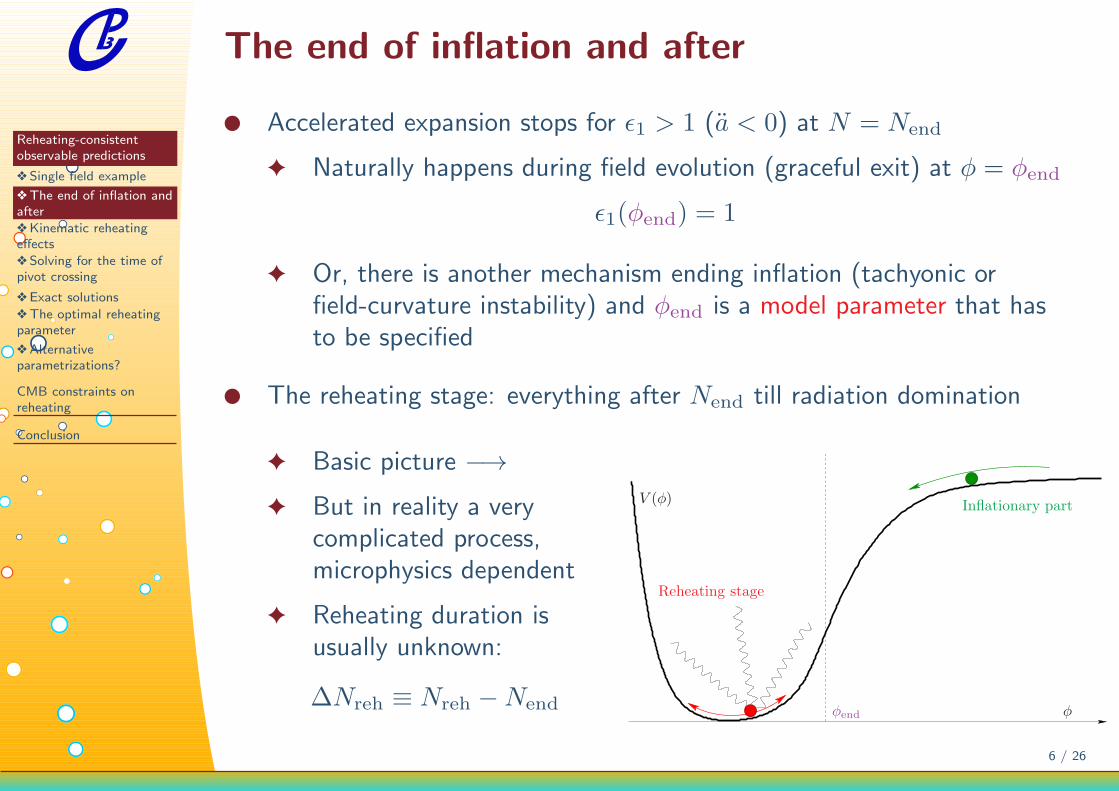
Accelerated expansion stops for ǫ1 > 1 (a < 0) at N = Nend
Naturally happens during field evolution (graceful exit) at φ = φend
ǫ1(φend) = 1
Or, there is another mechanism ending inflation (tachyonic orfield-curvature instability) and φend is a model parameter that hasto be specified
The reheating stage: everything after Nend till radiation domination
Basic picture −→ But in reality a very
complicated process,microphysics dependent
Reheating duration isusually unknown:
∆Nreh ≡ Nreh −Nend
PSfrag replacements
V (φ) Inflationary part
φφend
Reheating stage
bC
bC
bC
bC
bC
bC
bC
bC
bC
bC
bCbC
bC
bC
bCbC
bC
bC
bC
bC
bC
bC
Redshift at which reheating ends
Reheating-consistentobservable predictions
Single field example
The end of inflation andafter
Kinematic reheatingeffects
Solving for the time ofpivot crossing
Exact solutions
The optimal reheatingparameter
Alternativeparametrizations?
CMB constraints onreheating
Conclusion
7 / 26
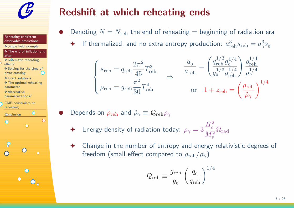
Denoting N = Nreh the end of reheating = beginning of radiation era
If thermalized, and no extra entropy production: a3rehsreh = a30s0
sreh = qreh2π2
45T 3reh
ρreh = grehπ2
30T 4reh
⇒
a0
areh=
(
q1/3rehg1/40
q1/30 g
1/4reh
)
ρ1/4reh
ρ1/4γ
or 1 + zreh =
(
ρrehργ
)1/4
Depends on ρreh and ργ ≡ Qrehργ
Energy density of radiation today: ργ = 3H2
0
M2P
Ωrad
Change in the number of entropy and energy relativistic degrees offreedom (small effect compared to ρreh/ργ)
Qreh ≡grehg0
(
q0qreh
)1/4

bC
bC
bC
bC
bC
bC
bC
bC
bC
bC
bC
bC
bC
Redshift at which inflation ends
Reheating-consistentobservable predictions
Single field example
The end of inflation andafter
Kinematic reheatingeffects
Solving for the time ofpivot crossing
Exact solutions
The optimal reheatingparameter
Alternativeparametrizations?
CMB constraints onreheating
Conclusion
8 / 26
Depends on the redshift of reheating
1 + zend =a0
aend=arehaend
(1 + zreh) =arehaend
(
ρrehργ
)1/4
=1
Rrad
(
ρendργ
)1/4
The reheating parameter Rrad ≡aendareh
(
ρendρreh
)1/4
Encodes any observable deviations from a radiation-like orinstantaneous reheating Rrad = 1
Rrad can be expressed in terms of (ρreh, wreh) or (∆Nreh, wreh)
lnRrad =∆Nreh
4(3wreh − 1) =
1− 3wreh
12(1 + wreh)ln
(
ρrehρend
)
where wreh ≡1
∆Nreh
∫ Nreh
Nend
P (N)
ρ(N)dN
A fixed inflationary parameters, zend can still be affected by Rrad

bC
bC
bCbC
bC
bC
bC
bC
bC
bC
bC
bCbC
bC
bC
bC
bC
bC
bC
bC
bC
bC
bC
bC
bC
bC
bC
bC
Reheating effects on inflationary observables
Reheating-consistentobservable predictions
Single field example
The end of inflation andafter
Kinematic reheatingeffects
Solving for the time ofpivot crossing
Exact solutions
The optimal reheatingparameter
Alternativeparametrizations?
CMB constraints onreheating
Conclusion
9 / 26
λ aα
areha*aeqaend
1/ H
Radiation MatterReheating
P(k)Nreh ?
Inflation
N=ln(a)
N* ~ 50−70 efolds
Nobs ~ 10 efolds
Model testing: reheating effects must be included!

bC
bC
bC
bC
bC
bC
bC
bC
bC
bC
bC
bC
bC
bC
bCbC
bC
bC
bC
bC
bC
Inflationary perturbations in slow-roll
Reheating-consistentobservable predictions
Single field example
The end of inflation andafter
Kinematic reheatingeffects
Solving for the time ofpivot crossing
Exact solutions
The optimal reheatingparameter
Alternativeparametrizations?
CMB constraints onreheating
Conclusion
10 / 26
Equations of motion for the linear perturbations
µT ≡ ahµS ≡ a
√2φ,Nζ
⇒ µ′′
TS +
[
k2 − (a√ǫ1)
′′
a√ǫ1
]
µTS = 0
Can be consistently solved using slow-roll and pivot expansion [Stewart:1993,
Gong:2001, Schwarz:2001, Leach:2002, Martin:2002, Habib:2002, Casadio:2005, Lorenz:2008, Martin:2013, Beltran:2013]
Pζ =H2
∗
8π2M2P
ǫ1∗
1 − 2(1 + C)ǫ1∗ − Cǫ2∗ +
π2
2− 3 + 2C + 2C
2
ǫ21∗ +
7π2
12− 6 − C + C
2
ǫ1∗ǫ2∗
+
π2
8− 1 +
C2
2
ǫ22∗ +
π2
24−
C2
2
ǫ2∗ǫ3∗
+
[
− 2ǫ1∗ − ǫ2∗ + (2 + 4C)ǫ21∗ + (−1 + 2C)ǫ1∗ǫ2∗ + Cǫ
22∗ − Cǫ2∗ǫ3∗
]
ln
(
k
k∗
)
+
[
2ǫ21∗ + ǫ1∗ǫ2∗ +
1
2ǫ22∗ −
1
2ǫ2∗ǫ3∗
]
ln2(
k
k∗
)
,
Ph =2H2
∗
π2M2P
1 − 2(1 + C)ǫ1∗ +
[
−3 +π2
2+ 2C + 2C
2]
ǫ21∗ +
−2 +π2
12− 2C − C
2
ǫ1∗ǫ2∗
+
[
−2ǫ1∗ + (2 + 4C)ǫ21∗ + (−2 − 2C)ǫ1∗ǫ2∗
]
ln
(
k
k∗
)
+(
2ǫ21∗ − ǫ1∗ǫ1∗
)
ln2(
k
k∗
)
Notice that: H∗ ≡ H(∆N∗) and ǫi∗ ≡ ǫi(∆N∗) with k∗η(∆N∗) = −1

bC
bC
bC
bC
bC
bC
bC
bC
bC
bC
bC
bC
bC
bC
bC bC
bC
bC
bC
bCbC
bC
bC
bC
bC
bC
bC
The power law parameters
Reheating-consistentobservable predictions
Single field example
The end of inflation andafter
Kinematic reheatingeffects
Solving for the time ofpivot crossing
Exact solutions
The optimal reheatingparameter
Alternativeparametrizations?
CMB constraints onreheating
Conclusion
11 / 26
From the observable point of view, one defines spectral index, running,tensor-to-scalar ratio, . . .
nS − 1 ≡ d lnPζ
d ln k
∣
∣
∣
∣
k∗
, αS ≡d2 lnPζ
d(ln k)2
∣
∣
∣
∣
k∗
, r ≡ Ph
Ph
∣
∣
∣
∣
k∗
They are read-off from the previous slow-roll expression
nS = 1− 2ǫ1∗ − ǫ2∗ − (3 + 2C)ǫ1∗ǫ2∗ − 2ǫ21∗ − Cǫ2∗ǫ3∗ +O(
ǫ3)
αS = −2ǫ1∗ǫ2∗ − ǫ2∗ǫ3∗ +O(
ǫ3)
r = 16ǫ1∗ (1 + Cǫ2∗) +O(
ǫ3)
One has to know the functions ǫi(∆N∗) and the value of ∆N∗ to makepredictions

bC
bC
bC
bC
bC
bC
bC
bC
Hubble-flow functions from the potential
Reheating-consistentobservable predictions
Single field example
The end of inflation andafter
Kinematic reheatingeffects
Solving for the time ofpivot crossing
Exact solutions
The optimal reheatingparameter
Alternativeparametrizations?
CMB constraints onreheating
Conclusion
12 / 26
One would prefer a “slow-roll” hierarchy based on V (φ) only
ǫv0(φ) ≡√
3
V (φ), ǫvi+1(φ) ≡
d ln ǫvi(φ)
dNwith
d
dN≡ −d lnV
dφ
d
dφ
Can be mapped with the Hubble flow hierarchy
ǫv0=
ǫ0√
1− ǫ1/3, ǫv1
= ǫ1
(
1 +ǫ2/6
1− ǫ1/3
)2
ǫv2 = ǫ2
[
1 +ǫ2/6 + ǫ3/3
1− ǫ1/3+
ǫ1ǫ22
(3− ǫ1)2
]
, ǫv3 = · · ·
Inversion can only be made perturbatively
ǫ1 = ǫv1 −1
3ǫv1ǫv2 −
1
9ǫ2v1ǫv2 +
5
36ǫv1ǫ
2v2
+1
9ǫv1ǫv2ǫv3 +O
(
ǫ4)
ǫ2 = ǫv2− 1
6ǫ2v2− 1
3ǫv2ǫv3− 1
6ǫv1ǫ2v2
+1
18ǫ3v2− 1
9ǫv1ǫv2ǫv3
+5
18ǫ2v2ǫv3
+1
9ǫv2ǫ2v3
+1
9ǫv2ǫv3ǫv4
+O(
ǫ4)
bC
bCbC
bC
bC
bC
bC
bC
bC
bC
bC
bC
bC
bC
bC
bCbC
bC
bC
bC
bC
bC
bC
bC
bC
bC
bCbC
bC
bC
bC
bC
bC
bC
bC bC
bC
Solving for the time of pivot crossing
Reheating-consistentobservable predictions
Single field example
The end of inflation andafter
Kinematic reheatingeffects
Solving for the time ofpivot crossing
Exact solutions
The optimal reheatingparameter
Alternativeparametrizations?
CMB constraints onreheating
Conclusion
13 / 26
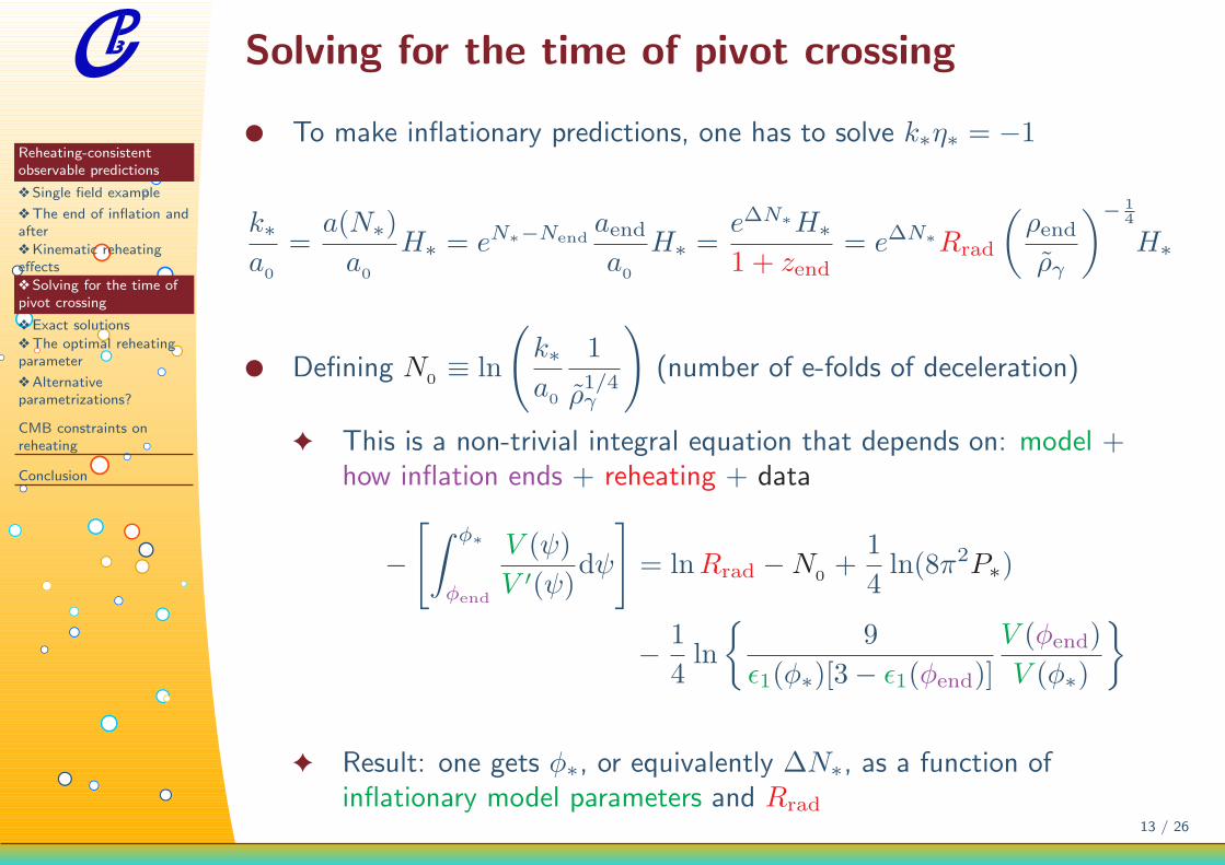
To make inflationary predictions, one has to solve k∗η∗ = −1
k∗a
0
=a(N∗)
a0
H∗ = eN∗−Nendaenda
0
H∗ =e∆N∗H∗
1 + zend= e∆N∗Rrad
(
ρendργ
)
−14
H∗
Defining N0≡ ln
(
k∗a0
1
ρ1/4γ
)
(number of e-folds of deceleration)
This is a non-trivial integral equation that depends on: model +how inflation ends + reheating + data
−[
∫ φ∗
φend
V (ψ)
V ′(ψ)dψ
]
= lnRrad −N0+
1
4ln(8π2P∗)
− 1
4ln
9
ǫ1(φ∗)[3− ǫ1(φend)]V (φend)
V (φ∗)
Result: one gets φ∗, or equivalently ∆N∗, as a function ofinflationary model parameters and Rrad

bC
bC
bC
bC
bC
bC
bC
bC
bC bC
bC
bC
bC
bC
bC
bC
bC
bC
bC
bC
bC
bC
Solving exactly for the perturbations
Reheating-consistentobservable predictions
Single field example
The end of inflation andafter
Kinematic reheatingeffects
Solving for the time ofpivot crossing
Exact solutions
The optimal reheatingparameter
Alternativeparametrizations?
CMB constraints onreheating
Conclusion
14 / 26
Inflationary dynamics given by (κ2 = 1/M2P)
S =
∫
dx4√−g
[
1
2κ2R+ L(φ)
]
with L(φ) = −1
2gµν∂µφ∂νφ− V (φ)
Knowing V (φ) + FLRW gives φ(N) (background); in turns φ(N) givesthe evolution of µS(η,k) ≡ a
√2φζ(η,k)
φ ≡ dφ
dN⇒ µS +
(
1− 1
2φ2)
µS +1
H2
[
(
k
a
)2
− (aφ)′′
a3φ
]
µS = 0
ζ is conserved after Hubble exit ⇒ Pζ(k)
What is the actual value of k/a to plug into this equation?
k/a = (k/a0)(1 + zend)eNend−N
The input are k/a0 (in Mpc−1) and Rrad
Exact integration requires Rrad (multifields included) [astro-ph/0605367,
astro-ph/0703486, arXiv:1004.5525]

bC
bC
bC
bC
bC
bC
bC
bC
bC
bC
bC
bC
bC
bC
bC
bC
bC
bCbC
bC
bC
bC
The optimal reheating parameter
Reheating-consistentobservable predictions
Single field example
The end of inflation andafter
Kinematic reheatingeffects
Solving for the time ofpivot crossing
Exact solutions
The optimal reheatingparameter
Alternativeparametrizations?
CMB constraints onreheating
Conclusion
15 / 26
Defining the rescaled reheating parameter [astro-ph/0605367]
lnRreh ≡ lnRrad +1
4ln ρend
“Magic” cancellation: Rreh absorbs the dependency in P∗ (valid out ofslow-roll and for multifields)
−[
∫ φ∗
φend
V (ψ)
V ′(ψ)dψ
]
= lnRreh −N0 −1
2ln
[
9
3− ǫ1(φend)V (φend)
V (φ∗)
]
What are the possible values of Rreh?
Within a given microphysics model, Rreh would be a function ofcoupling constants and inflationary parameters
Without any information, assuming −1/3 < wreh < 1 andρnuc ≡ (10MeV)4 < ρreh < ρend
−46 < lnRreh < 15 +1
3ln ρend

bC
bC
bC
bC
bC
bC
bC
bC
bC
bC
bC
bC
bC
bC
bC
bC
bC
bC
bC
bC
bC
bC
Example with Higgs and Starobinski inflation
Reheating-consistentobservable predictions
Single field example
The end of inflation andafter
Kinematic reheatingeffects
Solving for the time ofpivot crossing
Exact solutions
The optimal reheatingparameter
Alternativeparametrizations?
CMB constraints onreheating
Conclusion
16 / 26
Same potential: V (φ) ∝(
1− e−√
2/3φ/MP
)2
Starobinski Inflation: ρ1/4reh≃ 109 GeV [Terada et al., arXiv:1411.6746]
Higgs Inflation: ρ1/4reh
. 1013 GeV?? [Garcia-Bellido et al., arXiv:0812.4624]

bC
bC
bC
bC
bC
bC
bC
bC
bC
bC
bC
bC
bC
bC
bC
bC
bC
bC
bC
bC
bC
bC
Example with Higgs and Starobinski inflation
Reheating-consistentobservable predictions
Single field example
The end of inflation andafter
Kinematic reheatingeffects
Solving for the time ofpivot crossing
Exact solutions
The optimal reheatingparameter
Alternativeparametrizations?
CMB constraints onreheating
Conclusion
16 / 26
Same potential: V (φ) ∝(
1− e−√
2/3φ/MP
)2

bC
bC
bC
bC
bC
bC
bC
bC
bC
bC
bCbC
bC
bC
bC
bC
Alternative parametrizations?
Reheating-consistentobservable predictions
Single field example
The end of inflation andafter
Kinematic reheatingeffects
Solving for the time ofpivot crossing
Exact solutions
The optimal reheatingparameter
Alternativeparametrizations?
CMB constraints onreheating
Conclusion
17 / 26
The large ∆N∗ limit (when it exists) leads to inaccurate predictions
Starobinski Inflation
V (φ) ∝(
1− e−√
2/3φ/MP
)2
0.940 0.945 0.950 0.955 0.960 0.965 0.970 0.975 0.980nS
0.001
0.002
0.003
0.004
0.005
0.006
0.007
0.008
r
SI Planck 2015
LiteBird
LiteCore 120
Optimal Core
slow roll
limit ∆N ∗ ≫ 1
40
44
48
52
56
60
64
68
∆N∗
Quartic Small Field Inflation
V (φ) ∝ 1− (φ/µ)4
0.940 0.945 0.950 0.955 0.960 0.965 0.970 0.975 0.980nS
10-3
10-2
r
SFI4 with µ=10MPl
Planck 2015
LiteBird
LiteCore 120
Optimal Core
slow roll
limit ∆N ∗ ≫ 1
50
55
60
65
70
75
80
85
90
∆N∗
∆N∗ without a potential is unpredictable...

bC
bC
bCbC
bC
bC
bC
bC
bC
bC bC
bC
bC
bC
bC
bC
bC
bC
bC
bC
bC
bC
bC
bC
bC
bCbC
bC
bC
bC
bC
bC
bC
CMB constraints on reheating
Reheating-consistentobservable predictions
CMB constraints onreheating
Data analysis in modelspace
Posteriors and evidences
Planck 2015 +BICEP2/KECK data
Reheating constraints
Kullback-Leiblerdivergence
Information gain fromcurrent and future CMBdata
Conclusion
18 / 26

bC
bC
bC
bC
bC
bCbC
bC
bC
Data analysis in model space
Reheating-consistentobservable predictions
CMB constraints onreheating
Data analysis in modelspace
Posteriors and evidences
Planck 2015 +BICEP2/KECK data
Reheating constraints
Kullback-Leiblerdivergence
Information gain fromcurrent and future CMBdata
Conclusion
19 / 26
Data should be analyzed within the parameter space of each model,including the reheating parameter: (θinf , Rreh)
Using the public code ASPIC of Encyclopaedia Inflationaris [arxiv:1303.3787]
(θinf , Rreh) −→ ASPIC −→ ǫi∗ −→
Pζ(k)
Ph(k)−→
CAMB
CLASS←→ CMB data
Name Parameters Sub-models V (φ)
HI 0 1 M4(
1− e−√
2/3φ/MPl
)
RCHI 1 1 M4(
1− 2e−√
2/3φ/MPl +A
I
16π2
φ√
6MPl
)
LFI 1 1 M4(
φMPl
)p
MLFI 1 1 M4 φ2
M2
Pl
[
1 + α φ2
M2
Pl
]
RCMI 1 1 M4(
φMPl
)2 [
1− 2α φ2
M2
Pl
ln(
φMPl
)]
RCQI 1 1 M4(
φMPl
)4 [
1− α ln(
φMPl
)]
NI 1 1 M4[
1 + cos(
φf
)]
ESI 1 1 M4(
1− e−qφ/MPl
)
PLI 1 1 M4e−αφ/MPl
KMII 1 2 M4(
1− α φMPl
e−φ/MPl
)
HF1I 1 1 M4
(
1 +A1φ
MPl
)2 [
1− 23
(
A1
1+A1φ/MPl
)2]
CWI 1 1 M4
[
1 + α(
φQ
)4ln(
φQ
)
]
LI 1 2 M4[
1 + α ln(
φMPl
)]
RpI 1 3 M4e−2√
2/3φ/MPl
∣
∣
∣e√
2/3φ/MPl − 1∣
∣
∣
2p/(2p−1)
DWI 1 1 M4
[
(
φφ0
)2− 1
]2
MHI 1 1 M4[
1− sech(
φµ
)]
RGI 1 1 M4 (φ/MPl)2
α+(φ/MPl)2
MSSMI 1 1 M4
[
(
φφ0
)2− 2
3
(
φφ0
)6+ 1
5
(
φφ0
)10]
RIPI 1 1 M4
[
(
φφ0
)2− 4
3
(
φφ0
)3+ 1
2
(
φφ0
)4]
AI 1 1 M4[
1− 2π arctan
(
φµ
)]
CNAI 1 1 M4[
3−(
3 + α2)
tanh2(
α√
2
φMPl
)]
CNBI 1 1 M4[
(
3− α2)
tan2(
α√
2
φMPl
)
− 3]
OSTI 1 1 −M4(
φφ0
)2ln
[
(
φφ0
)2]
WRI 1 1 M4 ln(
φφ0
)2
SFI 2 1 M4[
1−(
φµ
)p]
– 15 –
II 2 1 M4(
φ−φ0
MPl
)
−β−M4 β2
6
(
φ−φ0
MPl
)
−β−2
KMIII 2 1 M4[
1− α φMPl
exp(
−β φMPl
)]
LMI 2 2 M4(
φMPl
)αexp [−β(φ/MPl)
γ ]
TWI 2 1 M4
[
1−A(
φφ0
)2e−φ/φ
0
]
GMSSMI 2 2 M4
[
(
φφ0
)2− 2
3α(
φφ0
)6+ α
5
(
φφ0
)10]
GRIPI 2 2 M4
[
(
φφ0
)2− 4
3α(
φφ0
)3+ α
2
(
φφ0
)4]
BSUSYBI 2 1 M4
(
e√
6 φ
MPl + e√
6γ φ
MPl
)
TI 2 3 M4(
1 + cos φµ + α sin2 φ
µ
)
BEI 2 1 M4 exp1−β
(
−λ φMPl
)
PSNI 2 1 M4[
1 + α ln(
cos φf
)]
NCKI 2 2 M4
[
1 + α ln(
φMPl
)
+ β(
φMPl
)2]
CSI 2 1 M4
(
1−α φ
MPl
)
2
OI 2 1 M4(
φφ0
)4[
(
ln φφ0
)2− α
]
CNCI 2 1 M4[
(
3 + α2)
coth2(
α√
2
φMPl
)
− 3]
SBI 2 2 M4
1 +[
−α+ β ln(
φMPl
)](
φMPl
)4
SSBI 2 6 M4
[
1 + α(
φMPl
)2+ β
(
φMPl
)4]
IMI 2 1 M4(
φMPl
)
−p
BI 2 2 M4
[
1−(
φµ
)
−p]
RMI 3 4 M4[
1− c2
(
−12 + ln φ
φ0
)
φ2
M2
Pl
]
VHI 3 1 M4[
1 +(
φµ
)p]
DSI 3 1 M4
[
1 +(
φµ
)
−p]
GMLFI 3 1 M4(
φMPl
)p [
1 + α(
φMPl
)q]
LPI 3 3 M4(
φφ0
)p (
ln φφ0
)q
CNDI 3 3 M4
1+β cos
[
α
(
φ− φ0
MPl
)]2
– 16 –

bC
bC
bC
bC
bC
bC
bCbC
bC
bC
bC
bC
bC
bC
bC
bC
bC
bC
bC
bC
bC
bC
Speeding up posterior and evidence calculations
Reheating-consistentobservable predictions
CMB constraints onreheating
Data analysis in modelspace
Posteriors and evidences
Planck 2015 +BICEP2/KECK data
Reheating constraints
Kullback-Leiblerdivergence
Information gain fromcurrent and future CMBdata
Conclusion
20 / 26
Effective likelihood for slow-roll inflation
Requires only one complete data analysis (COSMOMC) to get
Leff(D|P∗, ǫi∗) =
∫
p(D|θcosmo, P∗, ǫi∗)π(θcosmo)dθcosmo
Use machine-learning algorithm to fit its multidimensional shape
For each modelM and their parameters θinf , Rreh
p(θinf , Rreh|D,M) =Leff [D|P∗(θinf , Rreh), ǫi∗(θinf , Rreh)]π(θinf , Rreh|M)
p(D|M)
All posteriors on (θinf , Rreh) can be obtained from Leff
Marginalizing Leff over (θinf , Rreh) gives the Bayesian evidence
In practice
BAYASPIC ≡ ASPIC + MULTINEST + Leff [arXiv:1312.2347]
1 cpu-hour per modelM

bC
bC
bC
bC
bC
bCbC
bC
bC
bCbC
bC
bC
Planck 2015 + BICEP2/KECK data
Reheating-consistentobservable predictions
CMB constraints onreheating
Data analysis in modelspace
Posteriors and evidences
Planck 2015 +BICEP2/KECK data
Reheating constraints
Kullback-Leiblerdivergence
Information gain fromcurrent and future CMBdata
Conclusion
21 / 26
Marginalizing over instrumental, astro and cosmo parameters
With polarization TT and TE + B = 32 dimensions
θcosmo =
Ωbh2,Ωdmh
2, 100θMC, τ,
ycal, AB,dust, βB,dust, ACIB217 , ξ
tSZ,CIB, AtSZ143 ,
APS100, A
PS143, A
PS143×217, A
PS217, A
kSZ, AdustTT100 , AdustTT
143 ,
AdustTT143×217, A
dustTT217 , AdustEE
100 , AdustEE100×143, A
dustEE100×217,
AdustEE143 , AdustEE
143×217, AdustEE217 , AdustTE
100 , AdustTE100×143,
AdustTE100×217, A
dustTE143 , AdustTE
143×217, AdustTE217 , c100, c217
.

bC
bC
bC
bC
bC
bCbC
bC
bC
bCbC
bC
bC
Planck 2015 + BICEP2/KECK data
Reheating-consistentobservable predictions
CMB constraints onreheating
Data analysis in modelspace
Posteriors and evidences
Planck 2015 +BICEP2/KECK data
Reheating constraints
Kullback-Leiblerdivergence
Information gain fromcurrent and future CMBdata
Conclusion
21 / 26
Marginalizing over instrumental, astro and cosmo parameters
With polarization TT and TE + B = 32 dimensions
2.96 3.04 3.12 3.20
ln(1010P ∗ )
−4.8
−4.0
−3.2
−2.4
−1.6log(ǫ
1)
0.000 0.015 0.030 0.045 0.060
ǫ2
2.96
3.04
3.12
3.20
ln(1010P
∗)
0.000 0.015 0.030 0.045 0.060
ǫ2
−4.8
−4.0
−3.2
−2.4
−1.6
log(ǫ
1)
0.000 0.015 0.030 0.045 0.060
ǫ2
−0.16
−0.08
0.00
0.08
0.16
ǫ 3
−0.16 −0.08 0.00 0.08 0.16
ǫ3
2.96
3.04
3.12
3.20
ln(1010P
∗)
−0.16 −0.08 0.00 0.08 0.16
ǫ3
−4.8
−4.0
−3.2
−2.4
−1.6
log(ǫ 1)

bC
bC
bC
bC
bC
bC
bC
bC
bC
bC
bC
bC
bC
bC
bC
bC
bC
bC
bC
bCbC
Posteriors on the reheating parameter
Reheating-consistentobservable predictions
CMB constraints onreheating
Data analysis in modelspace
Posteriors and evidences
Planck 2015 +BICEP2/KECK data
Reheating constraints
Kullback-Leiblerdivergence
Information gain fromcurrent and future CMBdata
Conclusion
22 / 26
For each model, we use the most generic parameterization: Rreh
Prior choice: Jeffreys’ on Rreh ⇔ flat on lnRreh with:
−46 < lnRreh < 15 +1
3ln ρend
Planck data put non-trivial constraints on many models
Examples: LI with V (φ) =M4 (1 + α lnφ)
prior
-40 -30 -20 -10 0 10ln(R
reh)
0
LI
posterior
-40 -30 -20 -10 0 10ln(R
reh)
0
Planck 2013Planck 2015 + BICEP2
LI

bC
bC
bC
bC
bC
bC
bC
bC
bC
bC
bC
bC
bC
bC
bC
bC
bC
bC
bC
bCbC
Posteriors on the reheating parameter
Reheating-consistentobservable predictions
CMB constraints onreheating
Data analysis in modelspace
Posteriors and evidences
Planck 2015 +BICEP2/KECK data
Reheating constraints
Kullback-Leiblerdivergence
Information gain fromcurrent and future CMBdata
Conclusion
22 / 26
For each model, we use the most generic parameterization: Rreh
Prior choice: Jeffreys’ on Rreh ⇔ flat on lnRreh with:
−46 < lnRreh < 15 +1
3ln ρend
Planck data put non-trivial constraints on many models
Examples: SBI with V (φ) =M4[
1 + φ4 (−α+ β lnφ)]
prior
-40 -30 -20 -10 0 10ln(R
reh)
0
SBI
posterior
-40 -30 -20 -10 0 10ln(R
reh)
0
Planck 2013Planck 2015 + BICEP2
SBI

bC
bC
bC
bC
bC
Kullback-Leibler divergence
Reheating-consistentobservable predictions
CMB constraints onreheating
Data analysis in modelspace
Posteriors and evidences
Planck 2015 +BICEP2/KECK data
Reheating constraints
Kullback-Leiblerdivergence
Information gain fromcurrent and future CMBdata
Conclusion
23 / 26
Measure of information gain for the reheating parameter
DKL =
∫
P (lnRreh|D) ln
[
P (lnRreh|D)
π(lnRreh)
]
d lnRreh
Compute DKL for about 200 models of inflationMi?
But some models provide a very poor fit to the data
Can be quantified by the Bayesian Evidence
p(Mi|D) = π(Mi)
∫
Leff π(θinf)π(lnRreh)dθinfd lnRreh
We use Bayes Factors (relative scale of Evidences) withnon-commital priors
Bi ≡p(Mi|D)
supj [p(Mj |D)]=
p(D|Mi)
supj [p(D|Mj)]

bC
bC
bC
bC
bC
bC
bC
bC
bC
bC
bCbCbC
bC
bC
bC
bC
bC
bC
bC
bC
bC
bC
bC
bC
bC
bC
bC
bC
bC
bC
Information gain from current CMB data
Reheating-consistentobservable predictions
CMB constraints onreheating
Data analysis in modelspace
Posteriors and evidences
Planck 2015 +BICEP2/KECK data
Reheating constraints
Kullback-Leiblerdivergence
Information gain fromcurrent and future CMBdata
Conclusion
24 / 26
Evidence weighted 〈DKL〉 ≡∑
i P (Mi|D)DKL(Mi) ≃ 0.82
10-3 10-2 10-1 100
Bayes factor B/Bbest
0.0
0.5
1.0
1.5
2.0
2.5In
form
ation g
ain
DKL (in
bits)
favoredweakly disfavoredmoderately disfavoredstrongly disfavored
Planck 2015 + BICEP2/KECK
−10
−20
−30
−40
0
10
⟨ lnRreh⟩

bC
bC
bC
bC
bC
bC
bC
Information gain from future CMB data
Reheating-consistentobservable predictions
CMB constraints onreheating
Data analysis in modelspace
Posteriors and evidences
Planck 2015 +BICEP2/KECK data
Reheating constraints
Kullback-Leiblerdivergence
Information gain fromcurrent and future CMBdata
Conclusion
25 / 26
LITEBIRD with B-mode detection
10-3 10-2 10-1 100
Bayes factor B/Bbest
0
1
2
3
4
5
Inform
ation gain D
KL (in bits)
favoredweakly disfavoredmoderately disfavoredstrongly disfavored
LITEBIRD SI + Planck 2013
−10
−20
−30
−40
0
10
⟨ lnRreh⟩

bC
bC
bC
bC
bC
bC
bC
Information gain from future CMB data
Reheating-consistentobservable predictions
CMB constraints onreheating
Data analysis in modelspace
Posteriors and evidences
Planck 2015 +BICEP2/KECK data
Reheating constraints
Kullback-Leiblerdivergence
Information gain fromcurrent and future CMBdata
Conclusion
25 / 26
LITEBIRD without B-mode detection
10-3 10-2 10-1 100
Bayes factor B/Bbest
0
1
2
3
4
5
Inform
ation gain D
KL (in bits)
favoredweakly disfavoredmoderately disfavoredstrongly disfavored
LITEBIRD MHI + Planck 2013
−10
−20
−30
−40
0
10
⟨ lnRreh⟩

bC
bC
bC
bC
bC
bC
bC
Information gain from future CMB data
Reheating-consistentobservable predictions
CMB constraints onreheating
Data analysis in modelspace
Posteriors and evidences
Planck 2015 +BICEP2/KECK data
Reheating constraints
Kullback-Leiblerdivergence
Information gain fromcurrent and future CMBdata
Conclusion
25 / 26
CORE with B-mode detection
10-3 10-2 10-1 100
Bayes factor B/Bbest
0
1
2
3
4
5
Info
rmation g
ain
DKL (in
bits)
favoredweakly disfavoredmoderately disfavoredstrongly disfavored
CORE-M5 SI Delensed
−10
−20
−30
−40
0
10
⟨ lnRreh⟩

bC
bC
bC
bC
bC
bC
bC
Information gain from future CMB data
Reheating-consistentobservable predictions
CMB constraints onreheating
Data analysis in modelspace
Posteriors and evidences
Planck 2015 +BICEP2/KECK data
Reheating constraints
Kullback-Leiblerdivergence
Information gain fromcurrent and future CMBdata
Conclusion
25 / 26
CORE without B-mode detection
10-3 10-2 10-1 100
Bayes factor B/Bbest
0
1
2
3
4
5
Info
rmation g
ain
DKL (in
bits)
favoredweakly disfavoredmoderately disfavoredstrongly disfavored
CORE-M5 MHI Delensed
−10
−20
−30
−40
0
10
⟨ lnRreh⟩

bC
bC
bC
bC
bC
bC
bC
bC
bC bC
Conclusion
Reheating-consistentobservable predictions
CMB constraints onreheating
Conclusion
26 / 26
Current CMB data constrain reheating by 1 bit
1 bit = answers if Rreh is small or large
1 bit = amount of information contained in one letter [Shannon:1951]
Many models would be more severely constrained (or ruled-out) ifreheating predictions could be (or would have been) done
lnRrad =∆Nreh
4(3wreh − 1)
Additional X-era,late-time entropy production,. . . are undistinguishablefrom the CMB and structure formation point of view
Effective parameter: Rreh −→ RrehRXRY
But can be disambiguated with GW direct detection:arXiv:1301.1778
Euclid and large scale galaxy surveys will provide even more informationon the reheating (work in progress. . . )