bayesian statistical data assimilation for ecosystem ... · bayesian statistical data assimilation...

Available online at www.sciencedirect.com

s 68 (2007) 439–456www.elsevier.com/locate/jmarsys

Journal of Marine System

Bayesian statistical data assimilation for ecosystem modelsusing Markov Chain Monte Carlo

Michael Dowd ⁎

Department of Mathematics and Statistics, Dalhousie University, Halifax, Nova Scotia, Canada B3H 3J5

Received 17 August 2006; received in revised form 13 January 2007; accepted 19 January 2007Available online 8 February 2007

Abstract

This study considers advanced statistical approaches for sequential data assimilation. These are explored in the context ofnowcasting and forecasting using nonlinear differential equation based marine ecosystem models assimilating sparse and noisy non-Gaussian multivariate observations. The statistical framework uses a state space model with the goal of estimating the time evolvingprobability distribution of the ecosystem state. Assimilation of observations relies on stochastic dynamic prediction and Bayesianprinciples. In this study, a new sequential data assimilation approach is introduced based on Markov Chain Monte Carlo (MCMC). Theecosystem state is represented by an ensemble, or sample, from which distributional properties, or summary statistical measures, canbe derived. The Metropolis-Hastings based MCMC approach is compared and contrasted with two other sequential data assimilationapproaches: sequential importance resampling, and the (approximate) ensemble Kalman filter (including computational comparisons).A simple illustrative application is provided based on a 0-D nonlinear plankton ecosystem model with multivariate non-Gaussianobservations of the ecosystem state from a coastal ocean observatory. TheMCMC approach is shown to be straightforward to implementand to effectively characterize the non-Gaussian ecosystem state in both nowcast and forecast experiments. Results are reported whichillustrate how non-Gaussian information originates, and how it can be used to characterize ecosystem properties.© 2007 Elsevier B.V. All rights reserved.

Keywords:Marine ecosystem models; Data assimilation; State space models; Monte Carlo; Prediction; MCMC; Ensemble Kalman filter; Sequentialimportance resampling; Ecological statistics; Stochastic models; Particle filters; Non-Gaussian; Differential equations

1. Introduction

Data assimilation is fundamentally a problem instatistical estimation, i.e. combining dynamical modelsand data to provide state or parameter estimates. Marineecosystem models for lower trophic levels (biogeochem-ical and plankton models) typically take the form of time-dependent nonlinear differential equations (Fennell andNeumann, 2004), and are known to exhibit a wealth ofcomplex dynamical behaviour (Huisman and Weissing,

⁎ Tel.: +1 902 494 1048; fax: +1 902 494 5130.E-mail address: [email protected].

0924-7963/$ - see front matter © 2007 Elsevier B.V. All rights reserved.doi:10.1016/j.jmarsys.2007.01.007

2001; Edwards, 2001). These ecosystem models aregenerally treated as deterministic, and frequently coupled,as interacting tracers, to physical oceanographicmodels toallow for transport and mixing (Oschlies and Schartau,2005). Stochastic elements enter ecosystem modelsthrough environmental forcing such as mixed layerdynamics or rapid fluctuations in the light environment(Marion et al., 2000; Edwards et al., 2004; Dowd, 2006).Observations of marine ecological state variables arecomplex data types coming from a variety of sources andsensors (e.g. satellites, water samples, moored andprofiling instruments), and characterized by being sparse,noisy and non-Gaussian in their distributions (Dickey,

mailto:[email protected]

http://dx.doi.org/10.1016/j.jmarsys.2007.01.007

440 M. Dowd / Journal of Marine Systems 68 (2007) 439–456

2003). A major challenge for marine prediction is theidentification and development of appropriate dataassimilation methods to integrate this variety of datasources with marine ecosystem models.

Oceanographic data assimilation has generally beendivided into two approaches: (i) variational methodsfor estimation of parameters (and initial conditions), and(ii) sequential methods for state estimation. Parameterestimation is concerned with model calibration: modelsare considered as deterministic functions of the para-meters, a cost function is then posed which measures thediscrepancy between the model and data, and optimiza-tion procedures are used to minimize it (Lawson et al.,1995; Vallino, 2000; Evans, 2003; Oschlies and Schartau,2005). Sequential methods, on the other hand, are recur-sive algorithms concerned with estimation of the ecolo-gical state as the system evolves through time, in otherwords nowcasting and forecasting (Bertino et al., 2003).After model calibration, these sequential approachesprovide the basis for biological forecasting systems thatare emerging as part of ocean observing systems (Allenet al., 2003; Pinardi et al., 2003). This study is concernedwith the identification and application of advanced statis-tical methods for sequential data assimilation for non-linear and non-Gaussian interdisciplinary oceanographicstudies.

The integration of modern statistical approaches intooceanographic data assimilation is in its infancy. Methodssuch as Markov Chain Monte Carlo (MCMC) have revo-lutionalized Bayesian statistical computation (Gelmanet al., 2003). Indeed, the data assimilation problem haslong been formulated from a probabilistic perspectiveusing Bayesian principles (Jazwinski, 1970; van Leeuwenand Evensen, 1996). However, for sequential dataassimilation, the main approach has been to formulateapproximate methods based on extensions of the Kalmanfilter to treat nonlinear systems. For example, Pham et al.(1997) introduced the singular evolutive extended Kal-man (SEEK) filter based on an EOF approximation of theupdating equations. A popular Monte Carlo approach isthe ensemble Kalman filter, or EnKF (Tsuji andNakamura, 1973; Evensen, 1994). This uses stochasticdynamic (Monte Carlo) prediction, but approximates theBayesian assimilation of observations with the Kalmanfilter updating equations. It has been widely used inoceanography (Evensen, 2003), including applications tomarine ecological data assimilation (Eknes and Evensen,2002; Allen et al., 2003; Natvik and Evensen, 2003). Anexact statistical approach for sequential data assimilationin nonlinear and non-Gaussian systems is sequentialimportance resampling, or SIR (Gordon et al., 1993;Kitagawa, 1996). SIR has become well established in the

statistical and signal processing literature (see texts byDoucet et al. (2001) and Ristic et al. (2004)), with a fewpilot applications in data assimilation in physical ocean-ography (van Leeuwen, 2003) and biogeochemicalmodelling (Losa et al., 2003).

In this study, an alternative statistical approach forsequential data assimilation is introduced based on anMCMC approach. Like SIR, but unlike the EnKF, theproposed MCMC method provides an exact solution forgeneral nonlinear and non-Gaussian data assimilation.The well-known drawback of the SIR algorithm is that theensemble that represents the system state can degeneratedue to the repeated resampling (or bootstrapping) stepsthat are fundamental to its operation (e.g. Arulampalamet al., 2002). In recent work (Dowd, 2006), a modificationto the SIR algorithm was proposed to alleviate this prob-lem of sample degeneracy by appending anMCMC post-processing step to the SIR algorithm. However, it wassubsequently realized that the MCMC ideas developed inDowd (2006) could be adapted to stand-alone as a usefuland novel approach for sequential data assimilation. Thisstudy explores this idea and develops and tests themethodology, with an emphasis on estimation of the non-Gaussian features of the ecological state.

The paper is structured as follows. Section 2 introducesthe statistical framework for treating the nowcasting andforecasting problems of sequential data assimilation. Italso outlines the MCMC approach, and contrasts it to theSIR and EnKF algorithms. Section 3 provides an illustra-tion of the method with a simple application to a 0-Dnonlinear plankton model using non-Gaussian multivar-iate observations from a coastal ocean observing system.It is shown how the non-normal distributional informationfor nowcasts and forecasts can be used to diagnose anddescribe properties of the ecosystem state variables. Thecomputational performance of the candidate data assim-ilation algorithms are also compared and contrasted. Adiscussion and conclusions are given in Section 4.

2. Methods

2.1. Problem statement

The statistical framework for ecological data assim-ilation is provided by the nonlinear and non-Gaussianstate space model (e.g. Dowd and Meyer, 2003),

xt ¼ ftðxt−1; ht; ntÞ ð1Þ
yt ¼ htðxt;/t; vtÞ ð2Þdefined for t=1,… T. The first equation (Eq. (1)) is astochastic difference equation representing a Markovian

Fig. 1. The data assimilation cycle showing a single stage transition ofthe ecological system. It starts with a nowcast distribution of the stateat time t−1, or p(xt−1|y1:t−1). This is used as the initial condition for aforecast to time t using model dynamics to yield the p(xt|y1:t−1).Finally, this forecast is combined with the observation yt to produce thedesired nowcast at time t, or p(xt|y1:t). See the text for further details.

441M. Dowd / Journal of Marine Systems 68 (2007) 439–456

transition over a unit time interval (from time t−1 totime t). It is identified with the numerical model for theecological dynamics. The ecosystem state variables attime t are contained in the vector xt, which also includesany spatial dimension (e.g. gridded fields being mappedinto vectors). The state evolution, or ecosystem dyna-mics, is embodied in the operator ft, which may be timedependent. The model depends on a set of parameters θtwhich includes static rate constants, as well as time-dependent parameters and forcing (including boundaryfluxes). The system noise nt includes stochasticelements due to environmental forcing; in the estimationcontext it can also be considered to incorporate modelerrors due to structural uncertainty in the governingequations.

The second equation (Eq. (2)) is the measurementequation which incorporates observations on all or partof the ecological state. The observation vector at time tis given by yt, but may not be defined for all times (i.e.missing values). Observations, yt, are related to theecosystem state, xt, through the measurement operatorht. This depends on a parameter set, θt, and the mea-surement errors vt. This allows for indirect and nonlinearrelations between the observations and the state (e.g.measuring optical properties and modelling phytoplank-ton). Note that the special case of direct measurementsof the complete ecosystem state implies that ht is theidentity matrix.

Designate the available observation set from times 1through T inclusive as y1:T=(y1′, y2′,…, yT′)′ (that is, westack the observation vectors). Suppose we are interest-ed in state estimates at some analysis time τ (i.e. for xτ).Three classes of time-dependent estimation problemscan be defined corresponding to hindcasting (τbT),nowcasting (τ=T) and forecasting (τNT). Statistically,these correspond to the problems of smoothing, filteringand prediction. In this study we focus on the filtering(nowcasting) and prediction (forecasting) problemsusing online recursive approaches for sequential stateestimation.

A complete description of the ecosystem state at anytime is given by the joint probability density function(pdf) of xt defined for t=1,…, T. These pdfs embody allinformation on the ecological state and are commonlysummarized in terms of measures of the central tendency(the mean or mode), uncertainty (variance), and higherorder moments such as skewness and kurtosis. Relation-ships between variables can also be summarized bymeasures of dependence, such as covariance. The goal ofthis study is to estimate the time evolving probabilitydistribution of the ecological state using both ecosystemmodels and measurement information.

The target quantity to be computed by the sequentialdata assimilation procedure is p(xt|y1:t), which is theconditional pdf for the ecological state given all theinformation (observations) up to and including time t(where t=1,…, T). This is referred to as the filter, ornowcast, density at time t. Note that while the condi-tioning in the pdf only explicitly considers theobservations, it is implicit that the following also bespecified: the model equations, ft, along with the para-meters (forcing), θt; the measurement operator, ht, withits parameters, ϕt; and the statistics of both the systemnoise, nt, and observation error, vt. Initial conditions, x0,must also be provided.

Sequential estimation of the ecosystem state can beconceptualized in the data assimilation cycle in Fig. 1. Itstarts with an estimate of the ecological state at the currenttime (i.e. a nowcast at time t−1). This is designated byp(xt−1|y1:t−1) which is the pdf of xt−1 using measurementsup to and including time t−1. Two steps are then taken.First, a prediction is made for time t using p(xt−1|y1:t−1) asthe initial conditions for the (stochastic) ecological modeldynamics in Eq. (1), including any external forcing orboundary conditions. This yields the predictive densityp(xt|y1:t−1). Second, suppose an observation yt becomesavailable at time t. This measurement information isblended with the accumulated information on xt con-tained in the forecast. This yields the nowcast at time t asp(xt|y1:t). For sequential data assimilation, a recursivesequence of these single stage transitions of the system isapplied to the entire analysis period of interest.

2.2. Analytic solution

The rules for manipulating the pdfs in order to carryout the prediction and measurement steps of the data

Fig. 2. Ensemble based representation of a probability distribution.The x-axis is the value of the state variable and the y-axis denotesprobability (probability density for the distributions, and probabilitymass for the particles). The standard normal with mean zero andvariance one is shown (solid line). The ensemble members or particles(short vertical lines) are shown in terms of their values (x-axis position)and their probability (height above x=0). The estimated kernelsmoothed density determined from the ensemble is also given (dashedline). Panel (a) shows the case of n=25 ensemble size, while panel(b) shows the n=250 case.


assimilation cycle are given by the following (c.f.Jazwinski, 1970). The prediction step is

pðxtjy1:t−1Þ ¼Z

pðxtjxt−1Þpðxt−1jy1:t−1Þdxt−1: ð3Þ

The predictive distribution p(xt|y1:t−1) is computed as aproduct of the nowcast distribution, p(xt−1|y1:t−1), and atransition density p(xt|xt−1). This latter quantity movesthe state forward one time step and is identified with themodel dynamics in Eq. (1). The measurement updatestep occurs at time t when observational information ytbecomes available. The updating relies on straightfor-ward application of Bayes' formula, i.e.

pðxtjy1:tÞ ¼ pðytjxtÞpðxtjy1:t−1Þpðy1:tÞ ð4Þ

and yields the desired nowcast density at time t. Notethat the joint pdf of the observations p(y1:t) in thedenominator acts simply as a normalizing constant andmodern computational Monte Carlo techniques (asbelow) do not require its evaluation. The nowcast den-sity at time t, p(xt|y1:t), (the posterior) is expressed as theproduct of the likelihood p(yt|xt) and the forecast densityat time t, p(xt|y1:t−1), (the prior). The likelihood can beevaluated based on the measurement Eq. (2).

These two steps can be combined into a singleexpression for the single stage transition of the dataassimilation cycle by substituting Eq. (3) into Eq. (4)to yield

pðxtjy1:tÞ~pðytjxtÞZ

pðxtjxt−1Þpðxt−1jy1:t−1Þdxt−1: ð5Þ

where the proportionality means that the denominatorcan be dropped. This equation provides the basis for theMarkov Chain Monte Carlo based sequential data as-similation procedure introduced below.

2.3. Numerical solutions

2.3.1. Sampling based solutionsNumerical solutions for sequential data assimilation

for the general nonlinear and non-Gaussian case relies onMonte Carlo methods (Kitagawa, 1987). These are basedon algorithms that generate samples or ensembles fromthe desired nowcast (and forecast) distributions. Theseensembles can then be used to reconstruct approxima-tions to the distributions of interest, or any summaryquantities desired (e.g. the mean and variance). Considera set of n realizations of the ecosystem state vector, each

of which is denoted by x(i) where i=1,…, n. Supposethis sample is drawn from the (multivariate) probabilitydistribution p(x), as designated by the notation

fxðiÞgfpðxÞ; i ¼ 1; N ; n:

Here, superscript i is an index which refers to the ithmember of the ensemble, and the curly braces refer to theentire set, or the ensemble itself. Hence, {x(i)} denotesthe sample from p(x) which has n elements. As theensemble size n→∞ it provides for an exact represen-tation of the pdf of the random variable x.

Fig. 2 shows a illustration of such an ensemble basedrepresentation of a pdf. Here, random samples of sizen=25 and n=250 have been drawn from the standardnormal distribution (the N(0,1)) using a random numbergenerator. The positions of these ensemble members(or particles) are shown on the graph. Given this ensem-ble, estimates for the underlying distributional para-meters (the sample mean and sample variance) can bedetermined and are shown on the plots. Clearly the larger


ensemble gives answers that are closer to the true meanand variance. The distribution itself can also be recon-structed from the smoothed and scaled histogram, orthrough kernel density estimation (Silverman, 1986). Itis seen in Fig. 2 that the larger ensemble yields anestimated pdf much closer to the standard normal. Thissimple idea of using samples to characterize distributionsis the basis for the Monte Carlo based data assimilationmethods outlined below.

This same sample based characterization of the eco-system state can be applied to the single stage transitionof the data assimilation cycle as follows. The startingpoint is an ensemble of n ecological states given as

fxðiÞt−1jt−1gfpðxt−1jy1:t−1Þ; i ¼ 1; N ; n ð6Þ

that represents the nowcast pdf at time t−1 (it is shownhow this is generated recursively below; for now assumethat it is given). The subscripting on x designates asample at time t−1 using information (data) up to andincluding time t−1. The target distribution of the se-quential estimation procedure is the nowcast ensembleat time t represented as

fxðiÞtjt gfpðxtjy1:tÞ; i ¼ 1; N ; n: ð7Þ

Monte Carlo methods can be used to carry out thetransition from Eq. (6) to Eq. (7) for sequential dataassimilation. Sequential importance resampling (Gordonet al., 1993; Kitagawa, 1996) offers an exact solution,while the ensemble Kalman filter (Tsuji and Nakamura,1973; Evensen, 1994) provides an approximate one.Markov Chain Monte Carlo methods are another pos-sible approach for exact solutions to the problem ofsequential data assimilation. However, these have notbeen widely applied except as part of more comprehen-sive SIR algorithms (Gilks and Berzuini, 2001; Lee andChia, 2002; Dowd, 2006). MCMC methods have not, tothe author's knowledge, been applied for sequential dataassimilation for marine systems. In the next section, aflexible and general Metropolis-Hasting based MCMCalgorithm is proposed for sequential data assimilation.

2.3.2. MCMC for sequential data assimilationMarkov Chain Monte Carlo (MCMC) methods are

numerical methods which evaluate Bayes' formula togenerate ensembles drawn from a desired posterior (ortarget) distribution (e.g. Gamerman, 1997; Gelmanet al., 2003). For Bayesian sequential data assimilation,Eq. (5) indicates that the desired target distribution isp(xt|y1:t), or the nowcast at time t. To obtain the pos-terior via generation of an ensemble {xt|t

(i)}, we eval-

uate Eq. (5) using a Metropolis-Hasting MCMCtechnique. The Metropolis-Hastings algorithm is thebasis for a general and flexible class of MCMCmethods (Metropolis et al., 1953; Hastings, 1970), andbelow it is tailored to treat the problem of sequentialdata assimilation.

The iterative procedure used to generate the targetensemble {xt|t

(i)} is as follows. Suppose we are at thei−1th iteration of the Metropolis-Hastings algorithmand so the associated ensemble member, xt|t

(i−1), isavailable. To generate the next member in the targetensemble, xt|t

(i), the following steps are taken:

1. Generate a candidate xt|t−1⁎ as a sample from the fore-cast density p(xt|y1:t−1). To do this, first randomlychoose one member of the nowcast ensemble at theprevious time {xt−1|t−1

(i) }, which is designated as xt−1|t−1⁎ .This is then used as an initial condition for a forecast ofthe stochastic dynamic model of Eq. (1), i.e.

x⁎tjt−1 ¼ f ðx⁎t−1jt−1; ht; n⁎t Þ; ð8Þwhere nt⁎ represents an independent realization of thesystem noise.

2. Calculate the probability of accepting the candidatex t|t−1⁎ as the ith ensemble member of the target dis-tribution, i.e. as xt|t

(i). This probability is computed as

a ¼ min 1;pðytjx⁎tjt−1Þpðytjxði−1Þtjt Þ

0@

1A: ð9Þ

3. Accept the candidate as the ith ensemble memberwith probability α. This is carried out according tothe following rule. Draw z from Uniform(0,1) distri-bution. Then

xðiÞtjt ¼x⁎tjt−1 if zVa

xði−1Þtjt if zNa

(

Therefore given a starting value xt|t(1), the algorithm

can be run n times (or indeed any number of times) togenerate the required ensemble {xt|t

(i)}, i=1,…, n. Thisprovides a draw from the target nowcast distribution attime t, p(xt|y1:t). Pseudo-code for this algorithm is givenin Appendix A.

The MCMC algorithm offers significant advantagesfor sequential data assimilation. First, it is easy to im-plement. Appendix A shows that to sequentially generatecandidates, the ecosystemmodel is called as a subroutine(called ModelForecast) for one step ahead stochasticdynamic prediction of a single ensemble member. Thecandidates are then included in the target ensemble using


a simple accept/reject rule. The acceptance probability(9) takes the form of a simple ratio of likelihoodssince here the candidates are drawn from the prior,p(xt|y1:t−1) (Chib and Greenberg, 1995). The secondadvantage is that the sequence generated is an inde-pendence chain (Tierney, 1994). Candidates are drawnindependently from the predictive density and so haveno dependence on the current state of the algorithm.Dependence only arises due to the fact that the chaindoes not necessarily move (or accept the new candi-date) every iteration so that ensemble members can berepeated. This makes the acceptance probability α isan important diagnostic for algorithm performance. Asa consequence of this independence, some well knownissues with MCMC are alleviated: the sequence effec-tively mixes to rapidly explore the state space; and the“burn-in” time is negligible since once the first candi-date is accepted, the chain is generating draws fromthe posterior.

2.3.3. Other candidate approachesHere, two other statistical approaches for sequential

data assimilation are briefly reviewed and contrasted tothe MCMC approach (computational comparisons aregiven in Section 3). The first method is sequentialimportance resampling (SIR), which, like MCMC, pro-duces exact solutions for sequential data assimilation.The interested reader is referred to Ristic et al. (2004) fordetails of the algorithm; summaries in a marine eco-logical context are given in Losa et al. (2003) and Dowd(2006). The second method considered, the ensembleKalman filter (EnKF), provides an approximate solutionfor sequential data assimilation; implementation detailsare given in Evensen (2003).

2.3.3.1. Sequential importance resampling. SIRinvolves separate evaluations of both the predictionstep (3) and the measurement step (4). The starting pointis again the ensemble {xt−1|t−1

(i) } drawn from the nowcastdensity at time t−1, p(xt−1|y1:t−1). Prediction can bebased on an ensemble forecast, i.e.moving each of the nensemble members forward one time step using thestochastic dynamical model (1), i.e.

xðiÞtjt−1 ¼ f ðxðiÞt−1jt−1; ht; nðiÞt Þ: i ¼ 1; N ; n: ð10Þ

However, note that other proposal densities (other thanthe prior or predictive density) are possible. In theabove, nt

(i) represents an independent realization of thesystem noise for the ith ensemble member. This yields anew ensemble {xt|t−1

(i) } which is a draw from the pre-dictive density p(xt|y1:t−1). The measurement step (4)

then starts with the ensemble {xt|t−1(i) }. Each of the n

ensemble members is assigned a weight w(i) accordingto the likelihood

wðiÞ ¼ pðytjxðiÞt−1jtÞ; i ¼ 1; N n: ð11Þ

That is, ensemble members that are close to observationswill be given a higher weight, while those that are moredistant will be given a smaller weight. The probabilitymodel used to evaluate the likelihood follows the mea-surement distribution in Eq. (2). To generate the required(target) ensemble {xt|t

(i)}, the ensemble {xt|t−1(i) } is resam-

pled (with replacement) wherein members are chosenwith a probability proportional to their weight.

This weighted resampling procedure is at the core ofthe SIR methods. Its main drawback is sample impov-erishment wherein ensemble members with high weightsare chosen more frequently and the resultant targetsample {xt|t

(i)} may contain many repeats. Much researcheffort has been aimed at developing modified SIRschemes which alleviate these problems (Gilks andBerzuini, 2001; Arulampalam et al., 2002; Dowd, 2006).

2.3.3.2. Ensemble Kalman filter. The ensemble Kal-man filter also evaluates the prediction and measure-ment steps separately. As with SIR, prediction relies onensemble forecasts via Eq. (10). However, the measure-ment step is simplified by using the Kalman filter up-dating equations which follow from the linear, Gaussianversion of the state space model (1)–(2).

To illustrate the procedure, consider a version ofEq. (2) describing a linear observation equation definedby a matrix H and having additive errors vt. Suppose theforecast ensemble {x t|t−1

(i) } is available. The ith ensemblemember of the target nowcast at time t is determined as

x̃ðiÞtjt ¼ xðiÞtjt−1 þ KðyðiÞt −HxðiÞtjt−1Þ; i ¼ 1; N ; n ð12Þ

and the resultant ensemble {x̃ t|t(i)} represents the nowcast at

time t. The tilde notation is used to emphasize that theensemble will not in general be a draw from p(xt|y1:t), butonly an approximation. As part of the updating procedure(12), a measurement ensemble {yt

(i)} has been introducedand is generated as yt

(i) =yt+vt(i) for i=1,…, n where vt

(i) isan independent realization of the observation error. TheKalman gainmatrixK has also been used and is defined as

K ¼ PH VðHPH Vþ RÞ−1 ð13Þ

with P and R being the sample covariance matrices of theforecast ensemble {xt|t−1

(i) } and the observation ensemble{yt

(i)}, respectively.


The ensemble Kalman filter therefore does notevaluate directly Bayes formula in Eq. (4). Rather itapproximates the result by using the Kalman gain toupdate each forecast ensemble member by taking its oldvalue and adding to it an increment based on thediscrepancy between the observation and the forecast.For some cases, the EnKF can be transformed to anexact procedure (Bertino et al., 2003; Evensen, 2003).However, general observation error processes as in (2)are not supported directly.

3. Application

3.1. Observations

Measurements of the ecosystem state are takenfrom an observing system in Lunenburg Bay, Canada(44.36°N, 64.26°W). Lunenburg Bay is a small (8 kmlong), shallow (max depth 20 m) tidal embayment.Observations for both phytoplankton and nutrients areavailable. Phytoplankton observations were derivedfrom optical time series at three locations in the bayusing the algorithm of Huot et al. (submitted forpublication). Observations on inorganic nitrogen in-cluded both nitrates and ammonia and were based onbiweekly water sampling at 5 stations in the bay. Unitsfor these ecological state variables were expressed inμmol nitrogen l−1.

Fig. 3. Observations on phytoplankton and nutrients in Lunenburg Bay for 20value on any given day is also shown (large circles).

Observations for phytoplankton, P, and nutrients, N,from Lunenburg Bay are shown in Fig. 3. Since littlecoherent spatial variation was evident (in either thevertical or horizontal) in these variables, their dailyvalues have been spatially pooled and are reportedas time series. Phytoplankton observations have somegaps but are generally available on a regular daily basis(since they are derived from ocean optical data). Themedian value cycles near 1 μmol N l−1 until afterday 250 when it rises to near two. Significant highfrequency variability is seen. In contrast, the in situnutrient observations are much more sparse and exhibitsignificant sampling variability with few clear trendsevident.

The multiple observations on P and N for any givenday were treated as replicates and used to identify theappropriate probability distributions and estimate their(time-varying) parameters. Only distributions whichsupport non-negative values for the concentrations wereconsidered. For the P observations, a gamma(ν, β) distri-bution was found to well characterize the observations.The scale parameter was determined to be β=0.025, andthe shape parameter ν varied daily and depends on themean level, μ, of the process (i.e. ν=μ /β). For the Nobservations, a lognormal distribution was chosen. Themean of this distribution varied daily and its standarddeviation, σ, was found the be related to the mean, μ,according the following regression equation: σ=0.67–

04. Available measurements are given by small black dots. The median


0.25μ. For days with too few replicates for distributionfitting, these relationships were assumed to be valid. Thegamma and lognormal distributions for P and N serve tospecify the observation Eq. (2), and hence the likelihoodused in the measurement step of Eq. (4) and elsewhere.

3.2. Ecological model

The prototype ecological model for Lunenburg Bayis a simple 0-D biogeochemical model with ecosystemcomponents: phytoplankton (P), nutrients (N) and de-tritus (D). These prognostic variables are defined withina finite volume and co-evolve according to the follow-ing equations:

dPdt

¼ NkN þ N

gP−kP2 þ eP ð14Þ

dNdt

¼ /D−N

kN þ NgP þ eN ð15Þ

dDdt

¼ −/Dþ kP2 þ eD: ð16Þ

The state variables are in nitrogen concentration units.All quantities used in this model are summarized inTable 1. The deterministic part of the model is a sim-plified version of Dowd (2005) and further details canbe found there. Additive dynamical noise (εP, εN, εD)is appended to each of the equations as non-con-servative source and sink terms (Bailey et al., 2004).

Table 1State variables and parameters in the ecosystem model

Quantity Units Value Definition

State variables (xt)P μmol nitrogen l−1 – Phytoplankton biomassN μmol nitrogen l−1 – Inorganic nutrientsD μmol nitrogen l−1 – Organic detritusγ d−1 – Phytoplankton growth rate

Parameters (θt)kN μmol nitrogen l−1 2.5 Half-saturation for N

uptake by Pλ μmol nitrogen

l−1 d−10.05 Grazing loss of P

ϕ(t) d−1 0.02–0.1 Remaining rate of Dto N

gseas(t) μmol nitrogenl−1 d−1

0–1 Seasonally varying growthrate

a d−1 0.1 Decay/memory for γ

Explicit functional dependence on time (t) is indicated for parameters,along with the range of their values. Here, l is litres and d is days.

These accounts for the exchange (advection and mix-ing) of ecosystem components with the far field, so thatEqs. (14)–(16) acts as an open system.

The daily averaged light-limited growth parameteris also considered stochastic and time dependent. Itevolves according to the (Langevin) equation

dgdt

¼ gseasðtÞ−agþ eg ð17Þ

where gseas(t) represents deterministic forcing corre-sponding to the maximum light limited growth ratecomputed using surface irradiance, attenuation, and aphotosynthesis–irradiance curves (c.f. Dowd, 2005). Theremaining terms are a decay term and a random forcingterm εγ. This stochastic dynamic parameter is treated asan additional state variable (Kitagawa, 1998; Dowd,2006). The decorrelation scale is set at 1 /a=10 days,matching the meterological band and accounting forthe effects of fluctuations in light levels and mixing onP growth.

This system of coupled, nonlinear stochastic dif-ferential Eqs. (14)–(17) was discretized to yield a sto-chastic difference equation corresponding to the systemmodel (1). A 4×1 vector thus describes ecosystemstate at any time t, i.e. xt=(Pt, Nt, Dt, γt)′. Initialconditions in the form of an initial ensemble must alsobe specified. These have simply been defined using anormal distribution (truncated to be non-negative) overa reasonable set of values. Note that once observationsare assimilated, initial condition have almost no effecton the subsequent analysis for this 0-D ecosystemmodel.

The system noise process for the ecosystem statevariables (εP, εN, εD) and the stochastic parameter (εγ)are assumed normally distributed, zero-mean, andindependent through time. The variance of εγ was setsuch that it had a level of 20% of the mean of theseasonal growth curve. To specify the variance for theecosystem state variables consider its interpretation assource and sink terms due to mixing. Denote εi,t as thesystem noise for the ith element of the state vector xt(similarly for xi,t). The quantity εi,t /Δt can then beidentified with the concentration flux in a time in-crementΔt. If we assume Fickian diffusion wherein thisflux into the finite volume scales as K×(Δxi,t), where Kis an exchange coefficient and Δxi,t is a concentrationdifference. Thus, var(εi,t) =Δt2 ×K2 ×Δxi,t

2 . For thisstudy, we assume K=0.5 day−1 (flushing time scale of2 days), and Δxi,t=0.2xi,t. Note that these system noiseterms have been added in such a way as to ensure non-negative concentrations.


3.3. State estimation

Implementation of the MCMC data assimilationmethod followed the pseudo-code of Appendix A. Fromthis algorithm it can been seen that there are two mainsubroutines: (i) ModelForecast which corresponds to theecological model and moves the ecosystem state forwardone time increment (note that this is done for eachmemberof the ensemble); and (ii) Assimilate which incorporatesavailable measurements according to Bayes theorem byapplying the accept/reject rule. The solutions obtained bythe MCMC algorithm were verified by comparison toanalytic solutions provided by the Kalman filter forsimple linear, Gaussian cases. The consistency of theMCMC and SIR solutions for the application here wasalso verified for very large ensemble sizes.

As a baseline run, a very large ensemble size ofn=250,000 was used to ensure a close match with the truetarget (posterior) distribution. (This is clearly an unreal-istic ensemble size for practical application, but was hereused to provide an “exact” solution which facilitatesassessment of convergence and computational propertiesof the algorithms in the next section). The acceptanceprobabilities of theMetropolis-HastingMCMC algorithmover time were examined and had a median of 0.65 withan inter-quartile range of 0.14. Occasionally lowacceptance probabilities were associated with abruptshifts in the values of themeasurements. This is consistentwith Bayes' formula being a measure of the overlap of

Fig. 4. State estimates for the ecosystem variables and the stochastic dynami90% confidence regions (gray shaded area). Median values for observations

the likelihood and the predictive density. Also notethat the algorithm as given can be easily altered to runlonger chains which may be themselves sub-sampled toyield the desired target ensemble.

Fig. 4 shows nowcast results from the sequentialMCMC estimation procedure for the ecosystem statevariables and the stochastic dynamic growth parameter.Two summary quantities are shown: the median and the90% confidence region. The observed P are clusteredtightly around the median state, and the confidenceregion contains most of the observations. The ecosystemstate variable N is also observable but with fewer andmuch noisier measurements, and hence wider confi-dence regions. Its blocky appearance is a result of thesequential nature of the data assimilation cycle whereinafter analysis, a (smooth) prediction of the state forwardin time is made (with variance growth) followed by anabrupt correction upon encountering the next observa-tions (with variance collapse). The influence of the Pmeasurements on the N state is evident since thesevariance adjustments are occurring at times with no Nobservations (e.g. at day 130 and 270). The unobservedstate variable D is similarly indirectly influenced by theP and N observations, but is smoothed and has a widerconfidence interval. The estimates for the dynamicgrowth parameter show the imposed deterministicseasonal cycle but also the fluctuations which are aconsequence of the need to alter the phytoplanktongrowth rate in a manner consistent with the observations.

c growth parameter. Each panel shows the median (solid line) and theon P and N are also shown (black dots).

Fig. 5. Skewness (panel a) and kurtosis (panel b) for the ecosystemvariables and the stochastic dynamic growth parameter.


Note that near the end of the integration period, mass isbeing added to the system (via the dynamical noiseterms) to account for the observed increases in P and N.

Fig. 5 shows the time evolution of the skewness andkurtosis over the analysis period. This is reported for the

Fig. 6. Marginal (diagonal plots) and joint distribution (off diagonal plots) foreported for the ecosystem state variables P, N and D and are based on kern

nowcast ecosystem state variables and the stochasticdynamic growth parameter (note that the first twostatistical moments, the mean and the variance, of thenowcast state are not reported since their values areevident from Fig. 4). These higher order statisticalmoments provide an indication of the extent of non-Gaussianity in the estimated pdf of the ecosystem state.For most of the analysis period, the state variable P hasskewness near zero and a kurtosis near three. Thisindicates that the nowcast P distribution is not so farfrom a normal distribution. The reason for this near-normality is that P is observed at nearly all analysistimes and the gamma distribution used to characterizedthese measurements itself resembles a normal. Thisfeature influences the results of the Bayesian dataassimilation with the nowcast pdf taking on features ofthe observation distribution. The remaining state vari-ables N, D and γ are more non-Gaussian: they are leftskewed, and the kurtosis is greater than three implyingthey have heavier tails (or are more outlier prone) thanthe normal distribution.

Another feature of Fig. 5 is the growth in theskewness and kurtosis between observation times, andits abrupt decrease at observation times (this is parti-cularly evident for the observed N, but also found inother state variables). This feature has the same originas the variance growth and collapse discussed above.These higher order moments grow between observation

r the nowcast (filter) distributions, p(xt|y1:t), for day t=245. These areel smoothed density estimates.


times due to nonlinear dynamical prediction (uncon-strained by observations) that generates non-Gaussiandistributions (e.g. Miller et al., 1999). At times whendirect observations of the state variables are available,the Bayesian assimilation reduces these higher mo-ments consistent with the postulated distributions of theobservations.

The sequential data assimilation procedure can alsobe used to construct probability distributions for theecosystem state at any given time. Fig. 6 shows themarginal and joint distributions for the nowcast eco-system state, p(xt|y1:t), at a particular analysis time(t being day 245). These distributions are con-structed by kernel smoothed density estimation. Themarginal distributions for P, N and D can be com-pared to the time series results reported for day 245in Figs. 4 and 5). At day 245, Fig. 6 indicates themarginal distribution for P is symmetric with skew-ness and kurtosis near that of a normal distribution.The marginal distributions for D and N are clearlynon-Gaussian being left skewed and with light tails.The joint distributions are a statement of the relationbetween the ecosystem state variables; at this analy-sis time they suggest little in the way of dependencestructure for the nowcast state variables.

To examine the role of nonlinear dynamical predictionin changing the probability distributions of the ecosystem

Fig. 7. Marginal (diagonal plots) and joint distribution (off diagonal plots) foron a τ=30 day forecast. These are reported for the ecosystem state variables

state, forecast (predictive) distributions are next consid-ered. Fig. 7 shows a predictive distribution for day 245based on a 30 day forecast (i.e. starting from day 215).Compared to the nowcast distribution in Fig. 6, themarginals of the forecast ecosystem state all have a largervariance and are all left skewed. The joint distributionsindicate a greater dependence structure (e.g. highercovariance). This latter feature is due to the fact that theforecasted state depends more on the linkages imposed onthe state variables by the ecological dynamics, and less onobservational information (a 30 day forecast suffices toeffectively ‘forget’ the observational information).

To further examine the relative roles of the dynamicsand the observations in setting the dependence structureamongst the ecosystem state variables consider thefollowing. The strength of the relationship between twoecosystem state variables can be measured by theirmutual information (e.g. Kantz and Schreiber, 2003),according to the formula,

Iðxi;t; xj;tÞ ¼Z Z

pðxi;t; xj;tjy1:tÞ

� logpðxi;t; xj;tjy1:tÞ

pðxi;tjy1:tÞpðxj;tjy1:tÞ dxi;tdxj;t:

Here I(xi,t,xj,t) designates the mutual information be-tween two of the ecosystem state variables xi,t and xj,t at

the forecast (predictive) distributions, p(xt+τ|y1:t), for day t=245 basedP, N and D and are based on kernel smoothed density estimates.


time t (here i and j are one of P, N, or D, and i≠ j) . Thismeasure may be thought of as a generalization of cor-relation (e.g. a correlation of 0.5 corresponds to a mutualinformation of 1.2 for variables that follow a bivariatenormal). However, unlike correlation it is not restrictedto measuring only linear relationships. The quantities onthe right hand side involve both the joint and marginaldistributions of the ecosystem state. These quantities areproduced as part of the statistical data assimilationprocedure, examples of which were given for a singleanalysis time in Figs. 6 and 7.

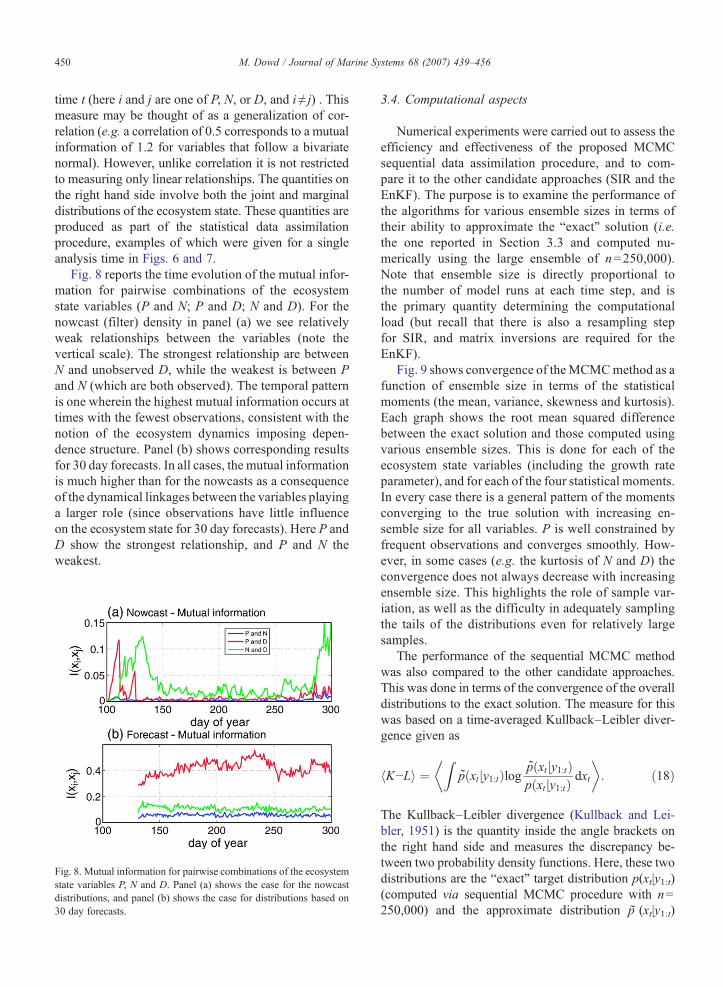
Fig. 8 reports the time evolution of the mutual infor-mation for pairwise combinations of the ecosystemstate variables (P and N; P and D; N and D). For thenowcast (filter) density in panel (a) we see relativelyweak relationships between the variables (note thevertical scale). The strongest relationship are betweenN and unobserved D, while the weakest is between Pand N (which are both observed). The temporal patternis one wherein the highest mutual information occurs attimes with the fewest observations, consistent with thenotion of the ecosystem dynamics imposing depen-dence structure. Panel (b) shows corresponding resultsfor 30 day forecasts. In all cases, the mutual informationis much higher than for the nowcasts as a consequenceof the dynamical linkages between the variables playinga larger role (since observations have little influenceon the ecosystem state for 30 day forecasts). Here P andD show the strongest relationship, and P and N theweakest.

Fig. 8. Mutual information for pairwise combinations of the ecosystemstate variables P, N and D. Panel (a) shows the case for the nowcastdistributions, and panel (b) shows the case for distributions based on30 day forecasts.

3.4. Computational aspects

Numerical experiments were carried out to assess theefficiency and effectiveness of the proposed MCMCsequential data assimilation procedure, and to com-pare it to the other candidate approaches (SIR and theEnKF). The purpose is to examine the performance ofthe algorithms for various ensemble sizes in terms oftheir ability to approximate the “exact” solution (i.e.the one reported in Section 3.3 and computed nu-merically using the large ensemble of n=250,000).Note that ensemble size is directly proportional tothe number of model runs at each time step, and isthe primary quantity determining the computationalload (but recall that there is also a resampling stepfor SIR, and matrix inversions are required for theEnKF).

Fig. 9 shows convergence of theMCMCmethod as afunction of ensemble size in terms of the statisticalmoments (the mean, variance, skewness and kurtosis).Each graph shows the root mean squared differencebetween the exact solution and those computed usingvarious ensemble sizes. This is done for each of theecosystem state variables (including the growth rateparameter), and for each of the four statistical moments.In every case there is a general pattern of the momentsconverging to the true solution with increasing en-semble size for all variables. P is well constrained byfrequent observations and converges smoothly. How-ever, in some cases (e.g. the kurtosis of N and D) theconvergence does not always decrease with increasingensemble size. This highlights the role of sample var-iation, as well as the difficulty in adequately samplingthe tails of the distributions even for relatively largesamples.

The performance of the sequential MCMC methodwas also compared to the other candidate approaches.This was done in terms of the convergence of the overalldistributions to the exact solution. The measure for thiswas based on a time-averaged Kullback–Leibler diver-gence given as

hK−Li ¼Z

p̃ðxtjy1:tÞlog p̃ðxtjy1:tÞpðxtjy1:tÞ dxt

� �: ð18Þ

The Kullback–Leibler divergence (Kullback and Lei-bler, 1951) is the quantity inside the angle brackets onthe right hand side and measures the discrepancy be-tween two probability density functions. Here, these twodistributions are the “exact” target distribution p(xt|y1:t)(computed via sequential MCMC procedure with n=250,000) and the approximate distribution p̃ (xt|y1:t)

Fig. 9. Convergence to the exact solution of the statistical moments (mean, variance, skewness, kurtosis) for the sequential MCMCmethod for each ofthe model variables. Results are reported as root-mean-square difference between approximate solution (calculated for various ensemble sizes) andthe exact solution.


(computed using various ensemble sizes and for eachof the three candidate sequential data assimilation ap-proaches). For reporting purposes, the Kullback–Leibler

Fig. 10. Convergence to the exact solution of the overall distribution as compthe time averaged Kullback–Leibler divergence for various ensemble sizes.considered for each of the four model variables.

divergence has been time averaged over the entireanalysis period, as denoted by the angle brackets inEq. (18). Fig. 10 shows the convergence of the different

uted by the sequential MCMC method. Results are reported in terms ofEach of the three candidate methods (the MCMC, SIR and EnKF) are


sequential data assimilation procedures to the targetdistribution as a function of the ensemble size. Both SIRand MCMC converge to the true solution with increas-ing ensemble size in an almost identical fashion. Asexpected, the (approximate) ensemble Kalman filterdoes not converge to the true solution with increasingensemble size. However, a notable point is that fornb1000 the ensemble Kalman filter appears to beslightly closer to the true solution than the other meth-ods. This is likely due to the smearing of the ensem-ble through use of the Kalman gain equations (vanLeeuwen, 2003). Note that raw unsmoothed and nor-malized histograms (not kernel smoothed density esti-mates) of the SIR and MCMC ensembles were used incomputing Eq. (18). However, by instead making use ofkernel smoothed density estimation (Silverman, 1986),this result might change.

To further examine the performance of the ensembleKalman filter, the convergence of the first two mo-ments (the mean and variance) is shown in Fig. 11.Higher order moments are not reported here since theEnKF is not intended to produce such estimates (in

Fig. 11. Convergence to the exact solution of the mean (panel a) andvariance (panel b) of the ensemble Kalman filter for each of the modelvariables. Results are reported as root-mean-square difference betweenapproximate solution (calculated for various ensemble sizes) and theexact solution.

fact, it was found that skewness and kurtosis from theEnKF in some cases actually diverged with increasingensemble size). The mean and variance of state vari-able P is best estimated, while the variable N is esti-mated poorly. However, while the mean and variancedo not converge to their true values with increas-ing ensemble size, they quickly reach an asymptoticequilibrium value. For the mean this occurs aftern=100, while for the variance it occurs after aboutn=1000.

4. Discussion and conclusions

Sequential data assimilation is of central interest forproblems in marine prediction, as well as the basis foremerging operational forecasting systems (Pinardiet al., 2003). This study examined advanced Bayesianstatistical data assimilation for nowcasting and forecast-ing in marine ecological systems. These approachesare designed to give full consideration to nonlineardynamics, as well as to emerging data types charac-terized by complex spatial and temporal structure andnon-normal distributions. Existing sequential dataassimilation techniques mainly rely on approximationsbased on the Kalman filter, usually involving linear-ization and/or dimension reduction (see Bertino et al.,2003). An alternative Monte Carlo based method is theensemble Kalman filter (Evensen, 2003). The EnKFapproximates the Bayesian measurement update step,and so cannot fully account for general non-Gaussianmeasurements. The more general case of strong dyna-mical nonlinearities and non-normal observational dis-tributions requires a fully Bayesian approach (Dowdand Meyer, 2003; van Leeuwen, 2003). The state spacemodel was put forth here as a comprehensive statis-tical framework for the data assimilation problem. Itsgeneral solution for the nonlinear and non-Gaussian casehas a Bayesian probabilistic formulation (Jazwinski,1970). Here, a novel and straightforward sequentialdata assimilation technique was offered based on aMarkov Chain Monte Carlo (MCMC) approach. Thisprovided for an exact solution in terms of a time evolv-ing ensemble (or sample) that represents the probabilitydensity function governing the multivariate ecologicalstate.

Markov Chain Monte Carlo (MCMC) methods are aclass of approaches for computational Bayesian statis-tics (e.g. Gamerman, 1997). They have revolutionalizedstatistical applications, but have been little applied to theproblem of oceanographic data assimilation. MCMChas, however, been used for parameter estimation inplankton models (Harmon and Challenor, 1997). Dowd


and Meyer (2003) also considered it for hindcastingusing a simple ecosystem model with general purposeBayesian software (BUGS, Spiegelhalter et al., 1995).There it was found that this Gibbs sampling MCMCsoftware was not readily tailored to time-dependentsystems used for dynamical modelling. In this study, itwas shown how the Metropolis-Hastings algorithmcan be adapted for sequential data assimilation. Thealgorithm is straightforward to apply with complexecosystem models, being highly modular and havingthe ecosystem model called simply as a subroutine. TheMCMC algorithm works simply through stochastic dy-namic prediction (ensemble forecasting), and a simpleacceptance/rejection rule for the assimilation of obser-vations. Unlike SIR, the approach does not rely onresampling and consequently does not exhibit sam-ple (ensemble) degeneracy, a problem that itself hasbeen the subject of a great deal of research effort(Arulampalam et al., 2002; Dowd, 2006). The MCMCdata assimilation approach introduced in this paperproduces an independence chain (Tierney, 1994), and soeffectively eliminates the well-known MCMC issues of“burn-in”, and facilitates mixing of the chain.

This study has repeatedly emphasized that ecologicalstate variables do not, as a rule, follow a normal distri-bution, but rather have a non-Gaussian structure that is notreadily described by parameteric probability distributions.It is well known that nonlinear models generate non-Gaussian distributions (Miller et al., 1999), as does theBayesian assimilation of non-normal observations. Toexamine these features, a test application was undertakenusing a 0-D nonlinear plankton ecosystem model andmultivariate non-Gaussian observations from a coastalocean observatory. Such a stochastic ecosystemmodel is acore element of the “weak constraint” approach, includingstochastic environmental variations as well as modelerrors (Marion et al., 2000; Dowd, 2006). The applicationalso treated an unknown parameter (the phytoplanktongrowth rate) as dynamic variable following a pre-definedstochastic process. The resultant ensemble that describedthe ecosystem state was used to construct marginal andjoint distributions of the ecosystem state variables. It wasalso used to compute summary statistics like the medianand confidence intervals, as well as measures of non-normality like skewness and kurtosis. It was shown howthe ecosystem model imposed dependence structure onthe ecosystem variables due to dynamical linkages(especially evident for forecasts). To effectively treat thenon-Gaussian information that emerges from this dataassimilation approach, some ideas from informationtheory have been suggested: mutual information provideda general measure for the dependence structure between

state variables; and the Kullback–Leibler divergence wasused to assess the convergence of the algorithms towardsthe true solution.

An important practical consideration for ensemblebased statistical data assimilation methods is their effi-ciency and effectiveness in characterizing the ecosystemstate. Towards this end, computational and convergenceproperties of various sequential Monte Carlo methods(MCMC, SIR and the EnKF) were examined in thecontext of a simple ecosystem model. It was found thatMCMC and SIR had similar convergence towards theexact solution. The approximate ensemble Kalman filteralso proved efficient with respect to recovering approx-imate values for the mean and the variance, at least untilthe ensemble size exceeded 100–1000, after which itcould no longer approach the true solution. The en-semble size is the primary determinant of the compu-tational load required for sequential data assimilation(SIR also requires resampling and the EnKF requiresevaluating matrix expressions and inverses). An impor-tant general point, which is demonstrated in the analysisof this study, is that the ensemble size required for dataassimilation will depend on the quantity desired. That is,an estimate for the mean state (or its variance) willrequire much smaller ensembles that if higher ordermoments (skewness or kurtosis) or full probability dis-tributions are of interest.

An outstanding research question is the extent towhich these ensemble based Bayesian data assimilationapproaches can be adapted for problems of more rea-listic dimensions, such as multi-compartment ecosystemmodels coupled to three-dimensional ocean circulationmodels (e.g. Oschlies and Schartau, 2005). In contrast tothe example in this study, these problems are describedby PDE based biophysical models with the state vectorcontaining spatial information on the prognostic eco-system models, and typically having dimensions of 105

or greater (the effective degrees of freedom is muchless). The challenge is to keep the ensemble size as smallas possible, while maintaining adequate performance ofthe data assimilation algorithm (this study providedsome general approaches to quantitatively measure thistradeoff.) For physical systems, Brusdal et al. (2003)applied an EnKF with a state vector of 106 and anensemble size of 150, and van Leeuwen (2003) used amodified SIR procedure with an ensemble size of 495and a state vector dimension of 2×105. Studies ofcoupled biophysical models using an EnKF have beensuccessful with ensemble sizes of 100 to 200 (Allenet al., 2003; Natvik and Evensen, 2003), while SIRbased applications have used ensemble sizes of 1000(Losa et al., 2003). The MCMC approach operates on


similar principles to SIR and should have comparableensemble size requirements.

All of the ensemble based sequential data assimi-lation methods rely on forecasting via Monte Carlointegration. They differ only in the way in which ob-servations are assimilated. The MCMC approach toBayesian data assimilation uses stochastic dynamic pre-diction after which the candidate ensemble member isevaluated for inclusion in the final ensemble (charac-terizing the target pdf) using an accept/reject step. Ingeneral, this procedure will preferentially accept ensem-ble members that are closest to the observations. Theacceptance probability is a key measure for the com-putational efficiency of Metropolis-Hastings methods(Chib and Greenberg, 1995). It will made highest whenforecasts closely match new observations. The systemnoise is a key determinant for maximizing the accep-tance probability as it dictates the spreading of theensemble and how many particle will intersect withregions of state space where the measurement pdf takeson non-negligible values. To improve ensemble fore-casts for Bayesian data assimilation other possibilitiesshould also be considered. For example, Chorin andKrause (2004) develop an approach to populate the statespace with particles (ensemble members) in the regionsinto which the dynamics are expanding. Another pos-sibility is to smear the ensemble by adding ‘jitter’ to theensemble members, or perhaps by sampling from kernelsmoothed density estimates or fitted parameteric formsof distributions. Adaptive approaches which use a var-iable ensemble size to ensure that the ensemble wellrepresents the ecosystem state are readily implementedvia the MCMC algorithm.

In summary, advanced statistical approaches for thedata assimilation problem are currently being widelyapplied in Statistics and Engineering. These treat generalnonlinear dynamics and non-Gaussian measurementsusing modern Bayesian computational approaches. It istimely to consider the adaptation of these approaches tooceanographic data assimilation. They are ideally suited toproblems in marine ecology and biogeochemistry due totheir strong nonlinearities and structural uncertainty, alongwith the need to use ecological measurements havingcomplex spatial and temporal structure. This study re-presents an initial step towards bringing these statisticalapproaches to bear on the data assimilation problem, andto allow researchers to consider non-Gaussian aspects ofthe problem. The implementation of these probabilisticapproaches to data assimilation is surprisingly straight-forward, and it is hoped that this work will encouragemarine modelling community to experiment with thesenovel statistical data assimilation procedures.

Acknowledgements

The author would like to thank many colleagues inboth Oceanography and Statistics for useful discussionincluding: John Cullen, Andy Edwards, Arnaud Doucet,Maud Guarracino, Chris Jones, Svetlana Losa, RenateMeyer, Bruce Smith, Keith Thompson, and Alain Ve-zina. This work was supported by an NSERC DiscoveryGrant, the National Program for Complex Data Struc-tures, and the Canadian Foundation for Climate andAtmospheric Science.

Appendix A. Pseudo-code for Metropolis-HastingsMCMC

⁎⁎Sequential MCMC data assimilation main program

FOR t=1 to TIF t is a measurement time

{xt|t(i)} = Assimilate(yt, {xt− 1|t − 1

(i) })ELSE IF t is NOT a measurement time

FOR i=1 to Nxt|t(i) =ModelForecast(xt − 1|t − 1

(i) , θt, nt(i))

END FOREND IF

END FOR

⁎⁎Subroutine for M-H MCMC measurement update

SUBROUTINE {xt|t(i)} = Assimilate(yt, {xt− 1|t− 1

(i) })- initialize xt|t

(1) (with, for example, yt or the median of{xt− 1|t− 1

(i) })FOR i=2 to N

- choose random pre-trial particle xt− 1|t − 1⁎ fromensemble {xt− 1|t− 1

(i) }- generate trial particlext|t − 1⁎ = ModelForecast(xt − 1|t − 1

⁎ , θt, nt⁎)- compute acceptance probability as:

a ¼ min 1;pðyt jx⁎tjt−1Þpðyt jxði−1Þtjt Þ

� �- draw z from Uniform(0,1) and set

xðiÞtjt ¼x⁎tjt−1 if zVa

xði−1Þtjt if zNa

(

END FORRETURN

References

Allen, J.I., Eknes, M., Evensen, G., 2003. An ensemble Kalman filterwith a complex marine ecosystem model: hindcasting phytoplank-ton in the Cretan Sea. Annales Geophysicae 21, 399–411.


Arulampalam,M.S.,Maskell, S., Gordon,N., Clapp, T., 2002.A tutorialon particle filters for online nonlinear/non-Gaussian Bayesiantracking. IEEE Transactions on Signal Processing 50 (2), 174–188.

Bailey, B., Doney, S.C., Lima, I.D., 2004. Quantifying the effects ofdynamical noise on the predictability of a simple ecosystem model.Environmetrics 15, 337–355.

Bertino, L., Evensen, G., Wackernagel, H., 2003. Sequential dataassimilation techniques in oceanography. International StatisticalReview 71 (2), 223–241.

Brusdal, K., Brankart, J.M., Halberstadt, G., Evensen, G., Brasseur, P.,van Leeuwen, P.J., Dombrowsky, E., Verron, J., 2003. Resultsfrom a comparison between the ensemble Kalman filter, the en-semble Kalman smoother, and the SEEK filter with real satelliteobservations in the North Atlantic, as performed in the DIADEM-project. Journal of Marine Systems 40–41, 253–289.

Chib, S., Greenberg, E., 1995. Understanding the Metropolis-Hastingsalgorithm. The American Statistician 49 (4), 327–335.

Chorin, A.J., Krause, P., 2004. Dimensional reduction for a Bayesianfilter. Proceedings of the National Academy of Sciences 101 (42),15013–15017.

Dickey, T.D., 2003. Emerging ocean observations for interdisciplinarydata assimilation systems. Journal of Marine Systems 40, 5–48.

Doucet, A., de Freitas, N., Gordon, N., 2001. Sequential Monte CarloMethods in Practice. Springer, New York. 581 pp.

Dowd, M., 2005. A biophysical coastal ecosystem model for assessingenvironmental effects of marine bivalve aquaculture. EcologicalModelling 183 (2–3), 323–346.

Dowd, M., 2006. A sequential Monte Carlo approach to marine eco-logical prediction. Environmetrics 17, 435–455.

Dowd, M., Meyer, R., 2003. A Bayesian approach to the ecosysteminverse problem. Ecological Modelling 169, 39–55.

Edwards, A.M., 2001. Adding detritus to a nutrient–phytoplankton–zooplankton model: a dynamical systems approach. Journal ofPlankton Research 23, 389–413.

Edwards, A.M., Platt, T., Sathyendranath, S., 2004. The high nutrient, lowchlorophyll regime of the ocean: limits on biomass and nitrate beforeand after iron enrichment. Ecological Modelling 171, 103–125.

Eknes, M., Evensen, G., 2002. An Ensemble Kalman filter with a 1-Dmarine ecosystem model. Journal of Marine Systems 36 (1–2),75–100.

Evans, G.T., 2003. Defining misfit between biogeochemical modelsand data sets. Journal of Marine Systems 40–41, 49–54.

Evensen, G., 1994. Sequential data assimilation with a non-linearquasigeostrophic model using Monte Carlo methods to forecasterror statistics. Journal of Geophysical Research 99, 10143–10162.

Evensen, G., 2003. The ensemble Kalman filter: theoretical formula-tion and practical implementation. Ocean Dynamics 53, 343–367.

Fennell, W., Neumann, T., 2004. Introduction to the Modelling ofMarine Ecosystems. Elsevier, Amsterdam. 330 pp.

Gamerman, D., 1997. Markov Chain Monte Carlo. Chapman & Hall/CRC, New York. 245 pp.

Gelman, A., Carlin, J.B., Stern, H.S., Rubin, D.B., 2003. BayesianData Analysis. Chapman and Hall/CRC, Boca Raton. 696 pp.

Gilks, W.R., Berzuini, C., 2001. Following a moving target — MonteCarlo inference for dynamic Bayesian models. Journal of the RoyalStatistical Society B 63 (1), 127–146.

Gordon, N.J., Salmond, D.J., Smith, A.F.M., 1993. Novel approach tononlinear/non-Gaussian Bayesian state estimation. IEE Proceed-ings-F 140 (2), 107–113.

Harmon, R., Challenor, P., 1997. AMarkov chainMonte Carlo methodfor estimation and assimilation into models. Ecological Modelling101, 41–59.

Hastings, W.K., 1970. Monte Carlo sampling methods using Markovchains and their applications. Biometrika 57, 97–109.

Huisman, J., Weissing, F.J., 2001. Biological conditions for oscilla-tions and chaos generated by multi-species competition. Ecology82, 2682–2695.

Huot, Y., Brown, C.A., Cullen, J.J., submitted for publication.Simultaneous inversion of reflectance, the diffuse attenu-ationcoefficient, and sun-induced fluorescence in coastal waters. Jour-nal of Geophysical Research.

Jazwinski, A.H., 1970. Stochastic Processes and Filtering Theory.Academic Press, New York. 376 pp.

Kantz, H., Schreiber, T., 2003. Nonlinear Time Series Analysis. Cam-bridge University Press, Cambridge. 386 pp.

Kitagawa, G., 1987. Non-Gaussian state-space modeling of nonsta-tionary time series. Journal of the American Statistical Association82, 1032–1041.

Kitagawa, G., 1996. Monte Carlo filter and smoother for non-Gaussiannonlinear state space models. Journal of Computational and Gra-phical Statistics 5, 1–25.

Kitagawa, G., 1998. A self-organizing state space model. Journal ofthe American Statistical Association 93 (443), 1203–1215.

Kullback, S., Leibler, R.A., 1951. On information and sufficiency.Annals of Mathematical Statistics 22 (1), 7986.

Lawson, L.M., Sptiz, Y.H., Hofmann, E.E., Long, R.L., 1995. A dataassimilation technique applied to a predator-prey model. Bulletinof Mathematical Biology 57, 593–617.

Lee, D.S., Chia, N.K.K., 2002. A particle algorithm for sequentialBayesian parameter estimation and model selection. IEEE Tran-sactions on Signal Processing 50 (2), 326–336.

Losa, S.N., Kivman, G.A., Schroter, J., Wenzel, M., 2003. Sequentialweak constraint parameter estimation in an ecosystem model.Journal of Marine Systems 43, 31–49.

Marion, G., Renshaw, E., Gibson, G., 2000. Stochastic modelling ofenvironmental variation for biological populations. TheoreticalPopulation Biology 57, 197–217.

Metropolis, N., Rosenbluth, A.W., Rosenbluth, M.N., Teller, A.H.,Teller, E., 1953. Equation of state calculations by fast computingmachines. Journal of Chemical Physics 21, 1087–1092.

Miller, R.N., Carter, E.F., Blue, S.T., 1999. Data assimilation intononlinear stochastic models. Tellus 51A, 167–194.

Natvik, L.J., Evensen, G., 2003. Assimilation of ocean colour datainto a biochemical model of the North Atlantic. Part 1. Dataassimilation experiments. Journal of Marine Systems 40–41,127–153.

Oschlies, A., Schartau, M., 2005. Basin-scale performance of a locallyoptimized marine ecosystem model. Journal of Marine Research63 (2), 335–358.

Pham, D., Verron, J., Roubaud, M., 1997. Singular evolutive Kalmanfilter with EOF initialization for data assimilation in oceanography.Journal of Marine Systems 16 (3–4), 323–340.

Pinardi, N., Allen, I., Demirov, E., De Mey, P., Korres, G., Lascaratos,A., Le Traon, P.-Y., Maillard, C., Manzella, G., Tziavos, C., 2003.The Mediterranean ocean forecasting system: first phase of imple-mentation (1998–2001). Annales Geophysicae 21, 3–20.

Ristic, B., Arulampalam, S., Gordon, N., 2004. Beyond the KalmanFilter: Particle Filters for Tracking Applications. Artech House,Boston.

Silverman, B.C., 1986. Density Estimation for Statistics and DataAnalysis. Chapman and Hall, New York.

Spiegelhalter, D.J., Thomas, A., Best, N.G., Gilks, W.R., 1995. BUGS:Bayesian Inference Using Gibbs Sampling, Version 0.50. MRCBiostatistics Unit, Cambridge.


Tierney, L., 1994. Markov chains for exploring posterior distributions(with discussion). Annals of Statistics 22, 1710–1762.

Tsuji, S., Nakamura, M., 1973. Nonlinear Filter using a statisticalprocessing technique. Transaction IEEJ (Institute of ElectricalEngineers of Japan) 93-C (5), 109–115.

Vallino, J.J., 2000. Improving marine ecosystem models: use of dataassimilation and mesocosm experiments. Journal of Marine Re-search 58, 117–164.

van Leeuwen, P.J., 2003. A variance-minimizing filter for large-scaleapplications. Monthly Weather Review 131, 2071–2084.

van Leeuwen, P.J., Evensen, G., 1996. Data assimilation and inversemethods in terms of a probabilistic formulation. Monthly WeatherReview 124, 2898–2913.

bayesian statistical data assimilation for ecosystem ... · bayesian statistical data assimilation...

Documents