bayesian reverse ecology using mutual information
TRANSCRIPT

Bayesian Reverse Ecology using MutualInformation
by
Suemin Lee
Thesis Submitted in Partial Fulfillment of theRequirements for the Degree of
Bachelor of Science
in theDepartment of Physics
Faculty of Science
c© Suemin Lee 2020SIMON FRASER UNIVERSITY
Spring 2020
Copyright in this work rests with the author. Please ensure that any reproductionor re-use is done in accordance with the relevant national copyright legislation.

Abstract
In stochastic biological systems, it is difficult to predict how the state of the system willevolve in response to a dynamic environment. Various attempts have been proposed indifferent literature. Some papers contain extreme simplicity in the system or suggest apotentially misleading method. In this study, we propose methodology to infer propertiesof the environment in which an observed system may have evolved: “reverse ecology”. Here,the system can be a cell, and the environment can be everything else other than the cell. Weaim to understand the success of a given system compared to all other possible systems inthe given environment. From this, we infer the environment that is the most likely one forthe system to have arisen in. This Bayesian approach is applied as an inference method thatis different from the existing methods. Two different model systems, Poisson distributionsand negative binomial distributions, are applied to infer the evolutionary environment froman observed system.
Keywords: Inference method, Mutual information
ii

Acknowledgements
First of all, I would like to express my deep gratitude to my supervisor, Dr.David Sivak,for allowing me to be part of his group. I appreciate all his patience, encouragement, guid-ance, and constant support throughout my undergraduate projects. His positive outlookand enthusiasm have inspired me to learn a lot about science and physics during my under-graduate studies. I sincerely thank him for being a wonderful supervisor over the past twoyears. Also, I would like to thank all the members of the Sivak group for their help duringmy thesis projects.
Also, I would like to thank my physics friends for their friendships, sharing joys andstudying and working assignments altogether. Also, I appreciate all the professors I havelearned from SFU across math and physics. Instead of mentioning individual names, I wouldlike to thank everyone who has helped me. If anyone reads my acknowledgement, I wouldlike to bring up their name here in this acknowledgement. Thank you for your help andyour support during my undergraduate.
Last but not least, I would like to express my sincere gratitude to my loving parents andmy brother for their patience and unconditional support during my undergraduate studies.I believe that undergraduate studies at SFU would not have been possible without theirhelp.
iii

Table of Contents
Abstract ii
Acknowledgements iii
Table of Contents iv
List of Tables vi
List of Figures vii
1 Introduction 11.1 Motivation . . . . . . . . . . . . . . . . . . . . . . . . . . . . . . . . . . . . 11.2 Background . . . . . . . . . . . . . . . . . . . . . . . . . . . . . . . . . . . . 2
1.2.1 Distributions of average number of proteins . . . . . . . . . . . . . . 21.2.2 Mutual information . . . . . . . . . . . . . . . . . . . . . . . . . . . 3
2 Method 52.1 Environment and system model setup . . . . . . . . . . . . . . . . . . . . . 52.2 Mutual Information between the Environment and System . . . . . . . . . . 6
2.2.1 General equation for mutual information . . . . . . . . . . . . . . . . 62.2.2 Mutual information for a system distribution according Poisson-distributed
system . . . . . . . . . . . . . . . . . . . . . . . . . . . . . . . . . . . 62.2.3 Mutual information for a system distribution according to the nega-
tive binomial . . . . . . . . . . . . . . . . . . . . . . . . . . . . . . . 72.2.4 Bayesian inference . . . . . . . . . . . . . . . . . . . . . . . . . . . . 7
3 Optimizing mutual information of environment with observed system 93.1 Poisson distribution . . . . . . . . . . . . . . . . . . . . . . . . . . . . . . . 93.2 Negative binomial distribution . . . . . . . . . . . . . . . . . . . . . . . . . 103.3 Limit of negative binomial distribution converging to Poisson distribution . 14
4 Comparing observed system to randomly sampled systems 154.1 Poisson distribution . . . . . . . . . . . . . . . . . . . . . . . . . . . . . . . 15
iv

4.1.1 Mutual Information distributions . . . . . . . . . . . . . . . . . . . . 154.1.2 Comparison on outperformance rate . . . . . . . . . . . . . . . . . . 16
4.2 Negative binomial distribution . . . . . . . . . . . . . . . . . . . . . . . . . 184.2.1 Mutual information distributions . . . . . . . . . . . . . . . . . . . . 184.2.2 Outperformance comparison . . . . . . . . . . . . . . . . . . . . . . . 184.2.3 Inference of optimal environmental probability . . . . . . . . . . . . 20
5 Conclusion and future works 225.1 Conclusion . . . . . . . . . . . . . . . . . . . . . . . . . . . . . . . . . . . . 225.2 Future works . . . . . . . . . . . . . . . . . . . . . . . . . . . . . . . . . . . 22
Appendix A Derivative of the mutual information 25A.1 Derivative of the Mutual information with respect to environmental proba-
bility derivation . . . . . . . . . . . . . . . . . . . . . . . . . . . . . . . . . . 25A.1.1 Mutual information derivative with respect to P (E) . . . . . . . . . 25A.1.2 Mutual information derivative with respect to p . . . . . . . . . . . 26A.1.3 Mutual information derivative evaluated at p=0.5. . . . . . . . . . . 26
A.2 Derivative of the Mutual information with respect to environmental proba-bility plots . . . . . . . . . . . . . . . . . . . . . . . . . . . . . . . . . . . . . 27A.2.1 Negative binomial distribution . . . . . . . . . . . . . . . . . . . . . 27
v

List of Tables
Table 3.1 Pmax for distinct ranges of system variables, for various burstiness pa-rameters b, for µ1=1 and µ2=17. . . . . . . . . . . . . . . . . . . . . . 12
vi

List of Figures
Figure 1.1 [A] Protein synthesis scheme leading to a Poisson distribution, withthe dynamical parameters b0 for protein production and g0 for pro-tein degradation. [B] Protein synthesis scheme leading to a negativebinomial distribution, with the dynamical parameters v0 for mRNAproduction, v1 for protein production, d0 for mRNA degradation,and d1 for protein degradation. . . . . . . . . . . . . . . . . . . . . 2
Figure 3.1 Mutual information of Poisson-distributed system with environment,as a function of probability Penv of high environmental state. Thesystem mean under one environmental state is µ = 1, with the othermean differing by ∆µ = [2, 4, 8, 16] in [A] to [D]. . . . . . . . . . . . 9
Figure 3.2 Mutual information between system and environment, as a func-tion of environmental probability Penv, for burstiness parameter b =5, 10, 20, 40 ([A] to [D]). . . . . . . . . . . . . . . . . . . . . . . . . . 11
Figure 3.3 Mutual information as a function of environmental probability Penv,computed across different system variable ranges and different bursti-ness parameters b = [5, 10, 20, 40] varying across columns. The sys-tem is distributed according to a negative binomial with mean µ=1or µ=17 depending on the environmental state. [A] Mutual informa-tion for observation s = 0; [B] range s = [1,∞); [C] entire systemvariable range s = [0,∞). . . . . . . . . . . . . . . . . . . . . . . . 12
Figure 3.4 Negative binomial distributions representing bursty protein produc-tion. The x-axis represents the system variable range, and the y-axisrepresents the probability for that number of proteins. [A] Fixedmean µ = 1, for varying burstiness parameter b. [B] Fixed meanµ = 17, for varying burstiness parameter b. . . . . . . . . . . . . . 13
Figure 3.5 Mutual information of a system with negative binomial distributionconverges at low burstiness parameter b to that of a system withPoisson distribution and same means. . . . . . . . . . . . . . . . . . 14
vii
Figure 4.1 Probability distribution of mutual information, for varying environ-mental probabilities Penv = 0.1 to Penv = 0.9, for system hyper-meanλ = 5 [A] and λ = 100 [B]. . . . . . . . . . . . . . . . . . . . . . . . 16
Figure 4.2 Outperformance proportion of the selected system as a function ofenvironmental probability. [A] and [B] share the same legend at fixedµ1 = 1 with change in µ2. [C] and [D] share the same legend at fixedµ2 = 1 with change in µ1. . . . . . . . . . . . . . . . . . . . . . . . 17
Figure 4.3 Mean (blue curves) and median (orange curves) of the distributionof mutual information, for system hyper-mean λ = 5. Burstinessparameter b = [5, 10, 20, 40] for [A]-[D]. . . . . . . . . . . . . . . . . 18
Figure 4.4 Outperformance proportion as a function of environmental proba-bility. [A] µ1 = 1 and µ2 = 3; [B] µ1 = 1 and µ2 = 5; [C] µ1 = 1and µ2 = 9; [D] µ1 = 1 and µ2 = 17 respectively. Random samplinghyper-mean is λ = 5. . . . . . . . . . . . . . . . . . . . . . . . . . . 19
Figure 4.5 Outperformance proportion of selected systems, as a function ofenvironmental probability. Burstiness parameter varies across b =[5, 10, 20, 40] in different-colored curves. The boxed subplots repre-sents Fig. 4.4. . . . . . . . . . . . . . . . . . . . . . . . . . . . . . . 20
Figure 4.6 Heat map of optimal environmental probability for the various se-lected systems distributed according to negative binomial. Burstinessparameter ranges across b = [5, 10, 20, 40] from [A] to [D]. . . . . . . 21
Figure A.1 Derivative of mutual information applied to negative binomial dis-tribution as a function of environmental probability. [A] Derivativeevaluated with mean of pair of µ1 =1 , µ2 =17. [B] Derivative evalu-ated with mean of pair of µ1 =17, µ2 =1. Different bursty parameterb evaluated for derivative of mutual information. . . . . . . . . . . . 28
Figure A.2 Derivative of mutual information applied to negative binomial dis-tribution evaluated at p=0.5 as a function of as a function of burstyparameter for single pair of mean values. . . . . . . . . . . . . . . . 28
viii

Chapter 1
Introduction
1.1 Motivation
The life of biological systems is stochastic. For stochastic systems, it is difficult to predicthow the state of the system will evolve in response to a dynamic environment. Variousattempts have been proposed in different literature to find systems that are evolutionarilyoptimized in response to a dynamic environment. Bowsher, et al. [1] propose an optimizedinference method by updating the results from a single input/output measurement. Also,Tkacik et al. [2] used a single gene responding to a transcription factor to track informationtransmission from the Bicoid/Hunchback system. In addition, Tkacik et al [3] predictedinference from dynamic system response to a dynamic environment using a simplified model.
Most of these studies applied an extremely simple model. Often this is beneficial forcomputational cost and obtaining the result quickly. Nevertheless, empirically we knowthat multiple organisms compete with one another to thrive in their given environment. Inorder to quantify the success of a biological system, one should also account for the otherpossible competitors it might face. The success of an organism is not determined by theabsolute standard of how good it is. Instead, the success should be defined by the relativecomparisons that it does better than other organisms.
In this paper, investigation of the methodology has been proposed to improve the in-ference method in reverse ecology using mutual information. We aim to understand howsuccessful a given system would be compared to all other possible systems in the givenenvironment. From this, we infer which environment is the most likely one for the systemto have arisen in.
The mutual information is used here to understand the success of the system in a givenenvironment. Mutual information quantifies the reduction in uncertainty of one variableby observing another variable. Therefore, calculating the mutual information between thesystem and several environments helps to understand the environment for which a givensystem is particularly well suited.
1

1.2 Background
1.2.1 Distributions of average number of proteins
Protein synthesis is one example of a stochastic system. Due to stochasticity, it is difficult topredict the exact quantity of a protein at a given time. Instead, we represent the number ofproteins in a cell, the result of protein synthesis and degradation dynamics, by a probabilitydistribution. Here, we describe two different model distributions of protein copy number,both simple and more complex models which closely approximate biological systems. Fig. 1.1provides a schematic of the protein production process.
b0<latexit sha1_base64="WpefCZSvzMVnFrTDozOagcVxXNg=">AAAB6nicbVBNS8NAEJ3Ur1q/qh69LBbBU0mqoMeCF48V7Ye0oWy2k3bpZhN2N0IJ/QlePCji1V/kzX/jts1BWx8MPN6bYWZekAiujet+O4W19Y3NreJ2aWd3b/+gfHjU0nGqGDZZLGLVCahGwSU2DTcCO4lCGgUC28H4Zua3n1BpHssHM0nQj+hQ8pAzaqx0H/TdfrniVt05yCrxclKBHI1++as3iFkaoTRMUK27npsYP6PKcCZwWuqlGhPKxnSIXUsljVD72fzUKTmzyoCEsbIlDZmrvycyGmk9iQLbGVEz0sveTPzP66YmvPYzLpPUoGSLRWEqiInJ7G8y4AqZERNLKFPc3krYiCrKjE2nZEPwll9eJa1a1buo1u4uK/XHPI4inMApnIMHV1CHW2hAExgM4Rle4c0Rzovz7nwsWgtOPnMMf+B8/gDw0o2k</latexit>
v0<latexit sha1_base64="NzM0HAb3vSSKuboEwHdltkauCrY=">AAAB6nicbVDLSgNBEOyNrxhfUY9eBoPgKexGQY8BQTxGNA9IljA7mU2GzM4uM72BsAT8AS8eFPHqF3nzb5w8DppY0FBUddPdFSRSGHTdbye3tr6xuZXfLuzs7u0fFA+PGiZONeN1FstYtwJquBSK11Gg5K1EcxoFkjeD4c3Ub464NiJWjzhOuB/RvhKhYBSt9DDqut1iyS27M5BV4i1ICRaodYtfnV7M0ogrZJIa0/bcBP2MahRM8kmhkxqeUDakfd62VNGIGz+bnTohZ1bpkTDWthSSmfp7IqORMeMosJ0RxYFZ9qbif147xfDaz4RKUuSKzReFqSQYk+nfpCc0ZyjHllCmhb2VsAHVlKFNp2BD8JZfXiWNStm7KFfuL0vV26d5HHk4gVM4Bw+uoAp3UIM6MOjDM7zCmyOdF+fd+Zi35pxFhMfwB87nDy+ijiU=</latexit>
v1<latexit sha1_base64="D/tXf91CvaAuszvLGxNROomvco4=">AAAB6nicbVDLSgNBEOyNrxhfUY9eBoPgKexGQY8BQTxGNA9IljA7mU2GzM4uM72BsAT8AS8eFPHqF3nzb5w8DppY0FBUddPdFSRSGHTdbye3tr6xuZXfLuzs7u0fFA+PGiZONeN1FstYtwJquBSK11Gg5K1EcxoFkjeD4c3Ub464NiJWjzhOuB/RvhKhYBSt9DDqet1iyS27M5BV4i1ICRaodYtfnV7M0ogrZJIa0/bcBP2MahRM8kmhkxqeUDakfd62VNGIGz+bnTohZ1bpkTDWthSSmfp7IqORMeMosJ0RxYFZ9qbif147xfDaz4RKUuSKzReFqSQYk+nfpCc0ZyjHllCmhb2VsAHVlKFNp2BD8JZfXiWNStm7KFfuL0vV26d5HHk4gVM4Bw+uoAp3UIM6MOjDM7zCmyOdF+fd+Zi35pxFhMfwB87nDzEmjiY=</latexit>
d0<latexit sha1_base64="6DVCYIUz90PTi+9umK2ds2h7GoU=">AAAB6nicbVDLSgNBEOz1GeMr6tHLYBA8hd0o6DEgiMeI5gHJEmZnZ5Mhs7PLTK8QloA/4MWDIl79Im/+jZPHQRMLGoqqbrq7glQKg6777aysrq1vbBa2its7u3v7pYPDpkkyzXiDJTLR7YAaLoXiDRQoeTvVnMaB5K1geD3xW49cG5GoBxyl3I9pX4lIMIpWug97bq9UdivuFGSZeHNShjnqvdJXN0xYFnOFTFJjOp6bop9TjYJJPi52M8NTyoa0zzuWKhpz4+fTU8fk1CohiRJtSyGZqr8nchobM4oD2xlTHJhFbyL+53UyjK78XKg0Q67YbFGUSYIJmfxNQqE5QzmyhDIt7K2EDaimDG06RRuCt/jyMmlWK955pXp3Ua7dPM3iKMAxnMAZeHAJNbiFOjSAQR+e4RXeHOm8OO/Ox6x1xZlHeAR/4Hz+ABQ2jhM=</latexit>
d1<latexit sha1_base64="2Y+KBMgJiDNtsOfHHj65yuaT+YE=">AAAB6nicbVDLSgNBEOz1GeMr6tHLYBA8hd0o6DEgiMeI5gHJEmZnZ5Mhs7PLTK8QloA/4MWDIl79Im/+jZPHQRMLGoqqbrq7glQKg6777aysrq1vbBa2its7u3v7pYPDpkkyzXiDJTLR7YAaLoXiDRQoeTvVnMaB5K1geD3xW49cG5GoBxyl3I9pX4lIMIpWug97Xq9UdivuFGSZeHNShjnqvdJXN0xYFnOFTFJjOp6bop9TjYJJPi52M8NTyoa0zzuWKhpz4+fTU8fk1CohiRJtSyGZqr8nchobM4oD2xlTHJhFbyL+53UyjK78XKg0Q67YbFGUSYIJmfxNQqE5QzmyhDIt7K2EDaimDG06RRuCt/jyMmlWK955pXp3Ua7dPM3iKMAxnMAZeHAJNbiFOjSAQR+e4RXeHOm8OO/Ox6x1xZlHeAR/4Hz+ABW6jhQ=</latexit>
[A] [B]
mRNA
DNA strand
DNA strand
ProteinProtein
g0<latexit sha1_base64="Ri+ii4A38TEGoVDer6TMVdj3/XU=">AAAB6nicbVDLSgNBEOz1GeMr6tHLYBA8hd0o6DEgiMeI5gHJEmYns5shs7PLTK8QloA/4MWDIl79Im/+jZPHQRMLGoqqbrq7glQKg6777aysrq1vbBa2its7u3v7pYPDpkkyzXiDJTLR7YAaLoXiDRQoeTvVnMaB5K1geD3xW49cG5GoBxyl3I9ppEQoGEUr3Uc9t1cquxV3CrJMvDkpwxz1Xumr209YFnOFTFJjOp6bop9TjYJJPi52M8NTyoY04h1LFY258fPpqWNyapU+CRNtSyGZqr8nchobM4oD2xlTHJhFbyL+53UyDK/8XKg0Q67YbFGYSYIJmfxN+kJzhnJkCWVa2FsJG1BNGdp0ijYEb/HlZdKsVrzzSvXuoly7eZrFUYBjOIEz8OASanALdWgAgwie4RXeHOm8OO/Ox6x1xZlHeAR/4Hz+ABjIjhY=</latexit>
DegradationDegradation
Degradation
Figure 1.1: [A] Protein synthesis scheme leading to a Poisson distribution, with the dy-namical parameters b0 for protein production and g0 for protein degradation. [B] Proteinsynthesis scheme leading to a negative binomial distribution, with the dynamical parame-ters v0 for mRNA production, v1 for protein production, d0 for mRNA degradation, and d1for protein degradation.
Poisson distribution
Simple protein regulation describes the birth and death process. In this model, the onlyexplicitly modeled events are protein synthesis and degradation. As denoted in Fig. 1.1[A],we let b0 be the production (birth) rate and g0 the degradation (death) rate. Suppose Np
is the number of proteins. The kinetic model summarized in Fig. 1.1[A] is described by thedynamical equation:
d〈Np〉dt
= b0 − g0〈Np〉 . (1.1)
2

By considering its steady-state solution, the mean protein copy number is computed as〈N ss
p 〉 = b0g0. At steady state the distribution is Poisson and denoted as [4]:
Poiss(b0g0
)=
(b0g0
)ss! e
−(b0g0
). (1.2)
Negative binomial distribution
The Poisson distribution results from a simple birth-death model of protein synthesis anddegradation. To more explicitly model gene expression requires an intermediate step in theproduction of protein, namely the production and degradation of mRNA. We denote v0 formRNA production, v1 for protein production, d0 for mRNA degradation, and d1 for proteindegradation. The gene expression described in Fig. 1.1[B] has equations:
d〈Nm〉dt
= v0 − d0〈Nm〉 (1.3a)
d〈Np〉dt
= v1〈Nm〉 − d1〈Np〉 (1.3b)
Examining the expressions for steady state, the mean mRNA is computed as 〈N ssm 〉 = v0
d0
and the mean protein is 〈N ssp 〉 = v1Nm
d1. The steady-state distribution resulting from this
kinetic scheme is the negative binomial distribution:
P
(n; a, b
1 + b
)= Γ(a+ n)
Γ(n+ 1)Γ(a)
(b
1 + b
)n (1− b
1 + b
)a. (1.4)
Here, a ≡ v0d1
is the typical number of mRNAs synthesized during a single protein lifetime,and b ≡ v1
d0is the burst size (or burstiness), the average number of proteins synthesized
from a single mRNA transcript. If b is large, a single mRNA molecule is typically translatedseveral times before that mRNA is degraded. If b = 1, each mRNA molecule is typicallytranslated only once. To understand more intuitively, when the typical number of mRNAa = 1 and the probability of r new proteins being produced is equal to the probability ofan mRNA being translated r times, this distribution is described as the burst/geometricaldistribution [5]:
p
(r; 1, b
1 + b
)=(
b
1 + b
)r (1− b
1 + b
). (1.5)
1.2.2 Mutual information
In information theory, Shannon introduced the entropy as a measure of uncertainty. Wedefine the concept of average uncertainty about random variable X that takes values x.The formula for the average uncertainty about X’s value is its entropy,
H(X) = −∑x
p(x) log2 p(x) (1.6)
3

Depending on the base of the given logarithm, entropy can have units of bits (base2), nats (base e), or dats (base 10) and the most common unit is bits with base 2. Thisdefinition is straightforwardly extended to two random variables X and Y .
The quantity called mutual information is:
I(X;Y ) =H(X)−H(X|Y ) (1.7)
=H(Y )−H(Y |X) (1.8)
=H(X) +H(Y )−H(X,Y ) . (1.9)
Here,H(Y |X) ≡
∑x
p(x)∑y
p(y|x) log2 p(y|x) (1.10)
is the conditional entropy and
H(X,Y ) ≡∑x,y
p(x, y) log2 p(x, y) . (1.11)
is the joint entropy.The mutual information between two variables X and Y can be understood as the gener-
alized correlation between these variables. More intuitively, it is the reduction in uncertaintyabout one variable provided by knowing another variable [6]. Considering two random vari-ables X and Y with a joint probability mass function p(x, y) and marginal probability massfunctions p(x) and p(y), the mutual information I(X;Y ) is the relative entropy betweenthe joint distribution p(x, y) and the product distribution p(x)p(y). Rewriting the mutualinformation in terms of the joint distribution of X and Y :
I(X;Y ) =∑x,y
p(x, y) log2p(x, y)p(x)p(y) . (1.12)
Comparing the joint probability p(x, y) and the product p(x)p(y) of the marginal probabil-ities p(x) and p(y), if X and Y are independent, these two distributions become equivalent.
4

Chapter 2
Method
The cell doesn’t have direct access to the external environment, and so can be thought ofas inferring the environmental state from observations of its own internal state, which wequantify by the intracellular number of the (signaling) protein. Here we derive expressions forthe mutual information between environment and system, for the two system distributions.
2.1 Environment and system model setup
We start with the simplest model to calculate mutual information between the environmentand the system. The environment is binary (high or low, or 1 or 2), and the system responseto a given environmental level is represented by a Poisson distribution or a negative binomialdistribution. The relationship between the environment and the system is
Environmental Distribution P (E) =
p E = High
(1− p) E = Low
System Response P (S|E) =
Poiss(µH) E = High
Poiss(µL) E = Low
or
System Response P (S|E) =
P (n; µHb ,b
1+b) E = High
P (n; µLb ,b
1+b) E = Low
Using the relationship between the environment and the system, mutual information iscalculated in the next section.
5

2.2 Mutual Information between the Environment and Sys-tem
2.2.1 General equation for mutual information
As introduced in Sec. 1.2.2, the mutual information formula is
I(S;E) =∑E=1,2
∞∑S=0
P (S,E) log2P (E,S)P (E)P (S) (2.1)
=∑E=1,2
∞∑S=0
P (S|E)P (E) log2P (S|E)P (S) (2.2)
=∑E=1,2
∞∑S=0
P (S|E)P (E) log2P (S|E)∑
E P (S|E)P (E) (2.3)
2.2.2 Mutual information for a system distribution according Poisson-distributed system
As described in Sec. 1.2.1, the Poisson distribution is
Poiss(µ) = µs
s! e−µ . (2.4)
The Poisson distribution (2.4) is substituted into the system response for each environmentalstate, P (S|E = 1) and P (S|E = 2), in the mutual information (2.3) to give
I(S;E) =∞∑S=0
P (S|E = 1)P (E = 1) log2P (S|E = 1)∑E P (S|E)P (E)
+∞∑S=0
P (S|E = 2)P (E = 2) log2P (S|E = 2)∑E P (S|E)P (E) (2.5)
=∞∑S=0
pµs1s! e−µ1 log2
µs1s! e−µ1
pµs1s! e−µ1 + (1− p) µ
s2s! e−µ2
+∞∑S=0
(1− p) µs2s! e−µ2 log2
µs2s! e−µ2
pµs1s! e−µ1 + (1− p) µ
s2s! e−µ2
(2.6)
=∞∑S=0
pµs1s! e−µ1
(− log2 p+ (1− p)
(µ2µ1
)se−(µ2−µ1)
)
+∞∑S=0
(1− p)µs2s! e−µ2
(− log2(1− p) + p
(µ1µ2
)se−(µ1µ2)
)(2.7)
6
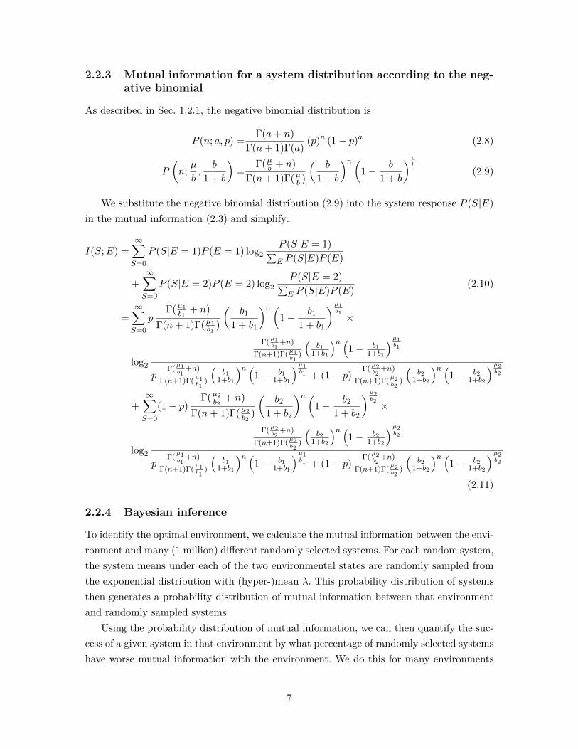
2.2.3 Mutual information for a system distribution according to the neg-ative binomial
As described in Sec. 1.2.1, the negative binomial distribution is
P (n; a, p) = Γ(a+ n)Γ(n+ 1)Γ(a) (p)n (1− p)a (2.8)
P
(n; µb,
b
1 + b
)=
Γ(µb + n)Γ(n+ 1)Γ(µb )
(b
1 + b
)n (1− b
1 + b
)µb
(2.9)
We substitute the negative binomial distribution (2.9) into the system response P (S|E)in the mutual information (2.3) and simplify:
I(S;E) =∞∑S=0
P (S|E = 1)P (E = 1) log2P (S|E = 1)∑E P (S|E)P (E)
+∞∑S=0
P (S|E = 2)P (E = 2) log2P (S|E = 2)∑E P (S|E)P (E) (2.10)
=∞∑S=0
pΓ(µ1
b1+ n)
Γ(n+ 1)Γ(µ1b1
)
(b1
1 + b1
)n (1− b1
1 + b1
)µ1b1 ×
log2
Γ(µ1b1
+n)Γ(n+1)Γ(µ1
b1)
(b1
1+b1
)n (1− b1
1+b1
)µ1b1
pΓ(µ1
b1+n)
Γ(n+1)Γ(µ1b1
)
(b1
1+b1
)n (1− b1
1+b1
)µ1b1 + (1− p)
Γ(µ2b2
+n)Γ(n+1)Γ(µ2
b2)
(b2
1+b2
)n (1− b2
1+b2
)µ2b2
+∞∑S=0
(1− p)Γ(µ2
b2+ n)
Γ(n+ 1)Γ(µ2b2
)
(b2
1 + b2
)n (1− b2
1 + b2
)µ2b2 ×
log2
Γ(µ2b2
+n)Γ(n+1)Γ(µ2
b2)
(b2
1+b2
)n (1− b2
1+b2
)µ2b2
pΓ(µ1
b1+n)
Γ(n+1)Γ(µ1b1
)
(b1
1+b1
)n (1− b1
1+b1
)µ1b1 + (1− p)
Γ(µ2b2
+n)Γ(n+1)Γ(µ2
b2)
(b2
1+b2
)n (1− b2
1+b2
)µ2b2
(2.11)
2.2.4 Bayesian inference
To identify the optimal environment, we calculate the mutual information between the envi-ronment and many (1 million) different randomly selected systems. For each random system,the system means under each of the two environmental states are randomly sampled fromthe exponential distribution with (hyper-)mean λ. This probability distribution of systemsthen generates a probability distribution of mutual information between that environmentand randomly sampled systems.
Using the probability distribution of mutual information, we can then quantify the suc-cess of a given system in that environment by what percentage of randomly selected systemshave worse mutual information with the environment. We do this for many environments
7

(parameterized by the probability of the high state) and ask for which environment thesystem outperforms the most (randomly sampled) systems. This approach allows us to findthe environment in which the observed system would be most competitive.
8

Chapter 3
Optimizing mutual information ofenvironment with observed system
Before making inferences, it is necessary to examine the mutual information between thesystem response and environment to understand behaviour. As introduced in Sec. 1.2, twoprotein distributions are used to model the system: the Poisson distribution and the nega-tive binomial distribution. After analysis of each distribution, we demonstrate that in theappropriate limit, the negative binomial asymptotes to a Poisson distribution.
3.1 Poisson distribution
Figure 3.1 shows numerical calculation of the mutual information (2.5) from Sec. 1.2, forPoisson system distributions with differences ∆µ = [2, 4, 8, 16] between the system averagesin the two environmental states. We find three basic trends.
0.2 0.4 0.6 0.8Penv
0.0
0.2
0.4
0.6
0.8
1.0
I(S;E
)
[A] 1 = 1 2 = 3 1 = 3 2 = 1
0.2 0.4 0.6 0.8Penv
0.0
0.2
0.4
0.6
0.8
1.0[B] 1 = 1 2 = 5
1 = 5 2 = 1
0.2 0.4 0.6 0.8Penv
0.0
0.2
0.4
0.6
0.8
1.0[C]
1 = 1 2 = 9 1 = 9 2 = 1
0.2 0.4 0.6 0.8Penv
0.0
0.2
0.4
0.6
0.8
1.0[D]
1 = 1 2 = 17 1 = 17 2 = 1
Figure 3.1: Mutual information of Poisson-distributed system with environment, as a func-tion of probability Penv of high environmental state. The system mean under one environ-mental state is µ = 1, with the other mean differing by ∆µ = [2, 4, 8, 16] in [A] to [D].
9

Three properties of mutual information for the Poisson distribution
First, the greater the difference between the means of the two pairs, the greater the mutualinformation. As the difference between means increases, the system distributions underdifferent environmental states grow more distinct. This greater separation increases theability to infer the environmental state from a given observation of the system state, andthus increases mutual information.
Another essential characteristic is that mutual information is a concave function, withthe maximum value of mutual information occurring around environmental probabilityPenv = 0.5. Also, it is minimized around Penv = 0.1 or 0.9. This is true because, whenPenv =0 or 1, the environment is not random, and uncertainty does not exist, leading tozero mutual information. Therefore, the mutual information minimizes around Penv=0.1or 0.9, and mutual information maximizes when the uncertainty between the two statesmaximize, corresponding to environmental probability around Penv=0.5.
Finally, the mutual information is symmetric after exchanging the order of the systemdistributions for the two environmental states. From Fig. 3.1, flipping the blue plot of themutual information around the y-axis at Penv = 0.5, gives the orange mutual informationplot. This has the same effect as changing the order between environmental state 1 andstate 2 because the environmental probability is associated with p and 1 − p in each stateso that it is symmetrical.
Therefore, for the Poisson distribution model, the larger the ∆µ, the greater the mutualinformation. In addition, the mutual information maximized (the system is most informa-tive) at environmental probability Penv = 0.5. Finally, the mutual information is symmetricwith respect to exchanging the order of the two means. These three features play an im-portant role in understanding the trends in the mutual information.
3.2 Negative binomial distribution
The main difference between Poisson and negative binomial distributions is that in thenegative binomial distribution, the model includes an additional description of the role ofmRNA in the protein production process. As a result, the negative binomial distributionintroduces an additional parameter b defining the ‘burstiness’. We vary b to change themutual information.
Change of mutual information
Figure 3.2 shows mutual information as a function of environmental probability, for fixedmean values and varying burst parameter b. As the burst parameter increases, the mutualinformation generally decreases. This decreasing mutual information can be explained bythe variance in the negative binomial distribution, which increases linearly with increasingburst parameters. The larger the variance, the wider the distribution and hence the larger
10

the overlap between the two different distributions. This overlapping region indicates thatthe two distributions are relatively indistinguishable for those system values. So when thedistributions more closely overlap, each observation has more similar probabilities in thetwo different distributions with different means, so each observation provides less informa-tion about which distribution it came from. Therefore, increased burstiness increases theuncertainty about the environmental state given a particular system observation.
0.2 0.4 0.6 0.8Penv
0.0
0.2
0.4
0.6
0.8
1.0
I(S;E
)
[A][A] 1 = 1 2 = 17 1 = 17 2 = 1
0.2 0.4 0.6 0.8Penv
0.0
0.2
0.4
0.6
0.8
1.0[B][B] 1 = 1 2 = 17
1 = 17 2 = 1
0.2 0.4 0.6 0.8Penv
0.0
0.2
0.4
0.6
0.8
1.0[C][C] 1 = 1 2 = 17
1 = 17 2 = 1
0.2 0.4 0.6 0.8Penv
0.0
0.2
0.4
0.6
0.8
1.0[D][D] 1 = 1 2 = 17
1 = 17 2 = 1
Figure 3.2: Mutual information between system and environment, as a function of environ-mental probability Penv, for burstiness parameter b = 5, 10, 20, 40 ([A] to [D]).
Symmetry change in mutual information
In addition to changes in mutual information, the symmetry of the mutual informationchanges as the means switch ordering for the same burstiness. In Fig. 3.2[A] to [D], theburstiness parameter increases, and within each subplot, the two curves have swappedordering of means and as a result swapped orderings of mutual information. As an example,within each individual subplot Fig. 3.2, the mutual information for µ1 = 1 and µ2 = 17(blue curve) has opposite ordering of mutual information compared to µ1 = 17 and µ2 = 1.In other words, the environmental probability that maximizes mutual information shifts tobelow or above Penv=0.5.
To understand the shift of information-maximizing environmental probability acrossPenv = 0.5, we closely examine mutual information for particular ranges of observations.This separation of outcomes helps to understand where information is acquired and whythe mutual information is maximized at a particular environmental probability Pmax. InFig. 3.3, we separate the system outcomes into two ranges, s = 0 and s = [1,∞), alsocomparing with the full mutual information over the entire range of outcomes, s = [0,∞).Table 3.1 tabulates these environmental probabilities that maximize mutual information.
When b = 5 or 10, the environmental probability that maximizes mutual informationremains the same for both the first and last rows (s = 0 and full-s range). This indicatesadding extra information gained from s = [1,∞) observations (Fig. 3.3[B]) does not change
11

0.2 0.4 0.6 0.80.0
0.2
0.4
0.6
0.8
1.0
I(S=0
; E)
[A][A][A][A][A][A][A][A][A][A][A][A]
b= 51=1 2 = 171=17 2 = 1
0.2 0.4 0.6 0.80.0
0.2
0.4
0.6
0.8
1.0b= 10
0.2 0.4 0.6 0.80.0
0.2
0.4
0.6
0.8
1.0b= 20
0.2 0.4 0.6 0.80.0
0.2
0.4
0.6
0.8
1.0b= 40
0.2 0.4 0.6 0.80.0
0.2
0.4
0.6
0.8
1.0
I(S=[
1,);
E)
[B][B][B][B][B][B][B][B][B][B][B][B]
0.2 0.4 0.6 0.80.0
0.2
0.4
0.6
0.8
1.0
0.2 0.4 0.6 0.80.0
0.2
0.4
0.6
0.8
1.0
0.2 0.4 0.6 0.80.0
0.2
0.4
0.6
0.8
1.0
0.2 0.4 0.6 0.8Penv
0.0
0.2
0.4
0.6
0.8
1.0
I(S; E
)
[C][C][C][C][C][C][C][C][C][C][C][C]
0.2 0.4 0.6 0.8Penv
0.0
0.2
0.4
0.6
0.8
1.0
0.2 0.4 0.6 0.8Penv
0.0
0.2
0.4
0.6
0.8
1.0
0.2 0.4 0.6 0.8Penv
0.0
0.2
0.4
0.6
0.8
1.0
Figure 3.3: Mutual information as a function of environmental probability Penv, computedacross different system variable ranges and different burstiness parameters b = [5, 10, 20, 40]varying across columns. The system is distributed according to a negative binomial withmean µ=1 or µ=17 depending on the environmental state. [A] Mutual information forobservation s = 0; [B] range s = [1,∞); [C] entire system variable range s = [0,∞).
Bursty parameter b Pmax for s = 0 Pmax for s = [1,∞) Pmax for s = [0,∞)5,10 Pmax < 0.5 Pmax > 0.5 Pmax < 0.520 Pmax < 0.5 Pmax > 0.5 Pmax = 0.540 Pmax < 0.5 Pmax > 0.5 Pmax > 0.5
Table 3.1: Pmax for distinct ranges of system variables, for various burstiness parameters b,for µ1=1 and µ2=17.
Pmax. When comparing s = 0 and entire s, Pmax remains in the same direction, so themutual information maintains the same symmetry.
b = 20 gives different results from b = 5 or 10. In Fig. 3.3[A], the mutual information ismaximized at the left side of Penv = 0.5 for blue curve and when extra information is addedfrom s = [1,∞), the mutual information is maximized at Penv = 0.5 in Fig. 3.3[C]. It followsthat, when the mutual information is maximizes at Penv = 0.5, the discrepancy betweenthe mutual information on two conjugate pairs of the mean (discrepancy between blue andorange curve) reduces to zero. This explains that the mutual informations are identical evenafter exchanging the system means for the two environmental states. Therefore, when themutual information maximizes at Penv = 0.5, it is symmetric around Penv = 0.5.
12

Finally, when b = 40, adding the information from the range s = [1,∞) causes Pmax
to cross over Penv = 0.5: Pmax is on one side of 0.5 for s = 0 and the other side fors = [0,∞). The discrepancy between the mutual information on conjugate pair betweenthe mean (difference between blue and orange curve) at s = 0 is relatively small comparedto s = [1,∞). Notice that the maximum mutual information (Pmax) at s = 0 is locatedon different position than s = [1,∞). Adding extra information gained from s = [1,∞)changes the position of the maximum mutual information (Pmax) for the entire range ofthe system. This shows that the Pmax is strongly influenced by the mutual information fors = 0. We conclude that the system outcome s = 0 is the governing case determining thesymmetry-breaking of mutual information.
The following claims can be further validated through more observations from Fig. 3.3:the discrepancy between the mutual informations for mean-swapped systems (blue andorange curves) is larger for s = 0 (Fig. 3.3[A]) than for s = [1,∞). The disparity in mutualinformation for s = [1,∞) remains relatively similar throughout the different burstinessparameters explored, whereas the disparity for s = 0 changes meaningfully with burstinessparameter. Therefore, we confirm that the system range s = 0 determines the symmetry-breaking of mutual information.
0 5 10 15 20
S variable
0
0.2
0.4
0.6
0.8
1
I(S
;E)
= 1 b= 5= 1 b= 10= 1 b= 20= 1 b= 40
0 10 20 30 40 50
S variable
0
0.05
0.1
0.15
0.2
0.25
= 1 b= 5= 1 b= 10= 1 b= 20= 1 b= 40
Figure 3.4: Negative binomial distributions representing bursty protein production. The x-axis represents the system variable range, and the y-axis represents the probability for thatnumber of proteins. [A] Fixed mean µ = 1, for varying burstiness parameter b. [B] Fixedmean µ = 17, for varying burstiness parameter b.
The statement is confirmed through direct inspection of the negative binomial distribu-tion (Fig. 3.4): when the burstiness parameter increases at fixed average, the distributionclusters more around s = 0 (higher probability systems variable s = 0). Thus at highburstiness, the system outcome is most likely zero. Since most of the distribution in eachenvironmental state is focused on zero, this reduces mutual information for s = 0 in thehigh-burstiness limit (Fig. 3.3).
13

In conclusion, for the negative binomial distribution, the symmetry of the mutual infor-mation changes by varying the burstiness parameter. Here, we found that the most decisiverole in determining the symmetry of the mutual information is the s = 0 outcome.
3.3 Limit of negative binomial distribution converging toPoisson distribution
The Poisson distribution is a simple limit of the negative binomial distribution: the negativebinomial distribution includes the Poisson distribution as a special case. The proof is intro-duced in Casella and Berger [7]. They use the characteristics of the Poisson distribution withthe same mean (µ) and variance (σ). In the negative binomial distribution, the relationshipbetween the mean (µ) and the variance (σ) approaching the same limit corresponds to:
E(X) = a p
(1− p) = ab→ µ (3.1)
Var(X) = a p
(1− p)2 = ab (1 + b)→ µ (3.2)
The statement follows, if a → ∞ and p → 0 such that a p = µ, (0 < µ < ∞), thenthe negative binomial distribution converges to the Poisson distribution as a limiting case.Here, p = b
1+b which p → 0, therefore it follows that b → 0. This is demonstrated inthe Fig. 3.5, which compares the mutual information of Poisson distribution and negativebinomial distributions with different b parameters.
0.2 0.4 0.6 0.8Penv
0.0
0.2
0.4
0.6
0.8
1.0
I(S;E
)
[A] PD 1 = 1 2 = 3 NBD b=0.01 NBD b=0.10 NBD b=1.00 NBD b=10.00 NBD b=100.00
0.2 0.4 0.6 0.8Penv
0.0
0.2
0.4
0.6
0.8
1.0[B] PD 1 = 1 2 = 5
0.2 0.4 0.6 0.8Penv
0.0
0.2
0.4
0.6
0.8
1.0[C] PD 1 = 1 2 = 9
0.2 0.4 0.6 0.8Penv
0.0
0.2
0.4
0.6
0.8
1.0[D] PD 1 = 1 2 = 17
Figure 3.5: Mutual information of a system with negative binomial distribution converges atlow burstiness parameter b to that of a system with Poisson distribution and same means.
Figure 3.5 shows that as b → 0, the negative binomial distribution closely approachesthe Poisson distribution. Also, we know that when b→ 0 then a→∞ since the mean value(µ = a b) is fixed. Therefore, Fig. 3.5 confirms that for b→ 0 with fixed µ (and hence witha→∞), the negative binomial converges to the corresponding Poisson distribution.
14
Chapter 4
Comparing observed system torandomly sampled systems
The Bayesian approach is another way of thinking about statistical inference. Bayesiananalysis allows us to infer an unknown environment by updating our beliefs about ran-dom variables. In the previous sections, we have investigated the behaviours of mutualinformation on different example distributions for responsive systems. In this section, werandomly sample systems to make comparisons with the observed system and understandits competitiveness. Through comparison in several different environments, we can infer theenvironment in which the observed system would be most competitive.
4.1 Poisson distribution
Assuming that proteins are Poisson distributed (which is a simple one-parameter distri-bution, but also the steady-state distribution for a simple birth-death model), we draw arandom sampling from exponential distributions to generate a distribution of mutual infor-mation.
4.1.1 Mutual Information distributions
In Chap. 3, we numerically computed the mutual information between a single systemand an environment. Following the same procedure, we generate a distribution of mutualinformation by calculating the mutual information between the environment and each of aset of randomly sampled systems. In the system distribution, λ represents the hyper-mean,the mean of the exponential distribution from which the system mean is drawn. By changingλ, different probability distributions are generated. In this example, we focus on analysis forλ = 5 and λ = 100. Choosing a larger λ shifts the system distribution to a higher mean andresults in a larger mean difference between the two pairs of states. This leads to a changein the mutual information distribution observed in Fig. 4.1.
15

0 0.2 0.4 0.6 0.8 1
I (S;E)
0
0.02
0.04
0.06
0.08
0.1
0.12
0.14
0.16
Pro
babi
lity
0 0.2 0.4 0.6 0.8 1
I (S;E)
0
0.1
0.2
0.3
0.4
0.5
0.6
0.7
Pro
babi
lity
0.1 0.2 0.3 0.4 0.5 0.6 0.7 0.8 0.9
Figure 4.1: Probability distribution of mutual information, for varying environmental prob-abilities Penv = 0.1 to Penv = 0.9, for system hyper-mean λ = 5 [A] and λ = 100 [B].
When the hyper-mean of the response system is small (λ = 5), the system distribu-tion is relatively densely concentrated at low mutual information values. In contrast, if thehyper-mean of the response system is large (λ = 100), the system distribution peaks nearthe maximum mutual information for each environmental probability. The reason followsdirectly from a single mutual information pair from Sec. 3.1. When the hyper-mean of thereaction system is small (λ = 5), the randomly chosen pair of means is also small, so mostsystem states are ambiguous as to the environmental state. Therefore, the average mutualinformation is significantly reduced. Conversely, when the hyper-mean of the response sys-tem is large (λ = 100), the mutual information between the system and the environmentbecomes large.
4.1.2 Comparison on outperformance rate
From the distribution of mutual information (Fig.4.1), we quantify the outperformance ofthe observed system in a given environment as the proportion of randomly sampled systemsthat produce lower mutual information than the observed system does. Figure 4.2 showsthis outperformance proportion as a function of environmental probability.
Both Fig. 4.2 [A] and [B] show that when µ2 > µ1, the system outperformance monoton-ically increases with environmental probability. In contrast, both Fig. 4.2 [C] and [D] showthat when µ1 > µ2, system outperformance monotonically decreases with environmentalprobability.
The monotonic increase and monotonic decrease occur due to the symmetry of the mu-tual information as a function of environmental probability. The distribution of mutualinformation for randomly sampled systems shows symmetry, i.e., is invariant to a change
16

0 0.2 0.4 0.6 0.8 10
20
40
60
80
100
0 0.2 0.4 0.6 0.8 10
20
40
60
80
100
0 0.2 0.4 0.6 0.8 10
20
40
60
80
100
1 = 1
2 = 3
1 = 1
2 = 5
1 = 1
2 = 9
1 = 1
2 = 17
0 0.2 0.4 0.6 0.8 10
20
40
60
80
100
1 = 3
2 = 1
1 = 5
2 = 1
1 = 9
2 = 1
1 = 17
2 = 1
Figure 4.2: Outperformance proportion of the selected system as a function of environmentalprobability. [A] and [B] share the same legend at fixed µ1 = 1 with change in µ2. [C] and[D] share the same legend at fixed µ2 = 1 with change in µ1.
of environmental probability from (Penv) to (1 − Penv). However, Sec. 3.1 showed that agiven system (with µ1 6= µ2) has mutual information asymmetric around Penv = 0.5. Theasymmetric mutual information of a given system and the symmetric mutual informationfor the distribution of systems correspond to monotonically increasing or decreasing out-performance: outperformance monotonically increases with environmental probability whenthe selected system has µ2 > µ1 and monotonically decreases when µ1 > µ2.
The analysis shows that the optimal environment for a given system is extreme (Popt =0.1 or Popt = 0.9), depending on the ordering of the means µ1 and µ2. Therefore, a Poissondistributed system is most competitive (is most likely to outcompete competing systemsand survive) in an extreme environment.
17

4.2 Negative binomial distribution
Incorporating further complexity to our model of the system, we examine how the optimalenvironment changes when the system has bursty protein production. As in the Poissondistribution, the average number of proteins is fixed, but there is now an additional modelparameter, the burstiness b. The inference method follows the same procedure as the Poissondistribution.
4.2.1 Mutual information distributions
0.2 0.4 0.6 0.8Penv
0.00
0.05
0.10
0.15
0.20
I(S;E
)
[A] b= 5
Mean Median
0.2 0.4 0.6 0.8Penv
0.00
0.05
0.10
0.15
0.20 [B] b= 10
Mean Median
0.2 0.4 0.6 0.8Penv
0.00
0.05
0.10
0.15
0.20 [C] b= 20
Mean Median
0.2 0.4 0.6 0.8Penv
0.00
0.05
0.10
0.15
0.20 [D] b= 40
Mean Median
Figure 4.3: Mean (blue curves) and median (orange curves) of the distribution of mutualinformation, for system hyper-mean λ = 5. Burstiness parameter b = [5, 10, 20, 40] for[A]-[D].
Figure 4.3 shows that the symmetry around Popt = 0.5 of the mutual information dis-tribution (at least as quantified by mean and median) is maintained for different burstinessparameters b. In the mean sampling distribution, the discrepancy between conjugate pairson environmental probabilities (Penv and (1−Penv) ) cancelled out, and it forms symmetricmutual information distribution. This indicates that the sampling distribution of the systemis equally beneficial between the symmetrical pairs of environmental probability.
Figure 4.3 also shows that the mean and median decrease for greater burstiness. In-tuitively, when burstiness is large, the system is more likely to produce a larger numberof proteins. Therefore, when proteins are produced with high burstiness at a fixed averagenumber, the system outcome is likely to be zero. Thus, regardless of the environmental state,the system outcome is likely to be the same, which simultaneously decreases the mean andthe median of the mutual information distribution.
4.2.2 Outperformance comparison
Figure 4.4 analyzes two important properties regarding different choices of a particular meanpair and different system burstiness. Figure 4.4[A] shows that, for fixed averages µ1 = 1and µ2 = 3 (and hence small mean difference ∆µ), changing the burstiness parameter doesnot greatly affect the curvature of the outperformance: outperformance still monotonically
18

0 0.2 0.4 0.6 0.8 138.5
39
39.5
40
40.5
41
41.5
42
42.5
43
b= 5b= 10b= 20b= 40
0 0.2 0.4 0.6 0.8 159
60
61
62
63
64
65
66
0 0.2 0.4 0.6 0.8 180
81
82
83
84
85
86
87
0 0.2 0.4 0.6 0.8 194.5
95
95.5
96
96.5
97
97.5
Figure 4.4: Outperformance proportion as a function of environmental probability. [A] µ1 =1 and µ2 = 3; [B] µ1 = 1 and µ2 = 5; [C] µ1 = 1 and µ2 = 9; [D] µ1 = 1 and µ2 = 17respectively. Random sampling hyper-mean is λ = 5.
increases with environmental probability. Conversely, Fig. 4.4[D] shows that for large meandifference ∆µ, the curvature of outperformance as a function of environmental probabilityis strongly affected by burstiness.
This demonstrates an effect of burstiness: when the burstiness parameter is large, theoutperformance is robust, maintaining the trend of increasing with Penv. In contrast, whenthe burstiness is small, the outperformance is less robust, shifting its curvature and therebychanging the optimal environmental probability.
Changes in outperformance occur for the same reasons as for the Poisson distribution.Notice the symmetry of the mutual information probability distribution for systems dis-tributed according to the negative binomial (Fig. 4.3). In contrast, Sec. 3.2 showed that themutual information between a given system and the environment was asymmetric in Penv,where the optimal environmental probability Pmax shifted with changing burstiness. Thechange in outperformance is explained by comparing the asymmetric mutual information ofthe given system to the symmetric mutual information distribution across randomly sam-pled systems. Therefore, the curvature of the outperformance trend follows the behaviourof the asymmetrical single mutual information.
As a result, Fig.4.4 shows that if the mean difference (∆µ) of the given pair is small,then the burstiness has less effect on outperformance: for large burstiness parameter, thecurvature of the outperformance remains steady. Both observations were supported by acomparison between the asymmetric mutual information for a given system and the sym-metry of the mutual information distribution.
Furthermore, to find a more generalized description of the optimal environmental prob-abilities, Fig.4.4 can be further extended by comparing more observed systems. Using thesame mutual information distribution, we compare selected systems with different means:µ1 = [1, 2, 4, 8, 16, 32] and difference ∆µ = [1, 2, 4, 8, 16, 32]( Fig. 4.5).
19

0.2 0.4 0.6 0.823
24
25
b=5 b=10 b=20 b=40
0.2 0.4 0.6 0.838
40
42
0.2 0.4 0.6 0.8
60
62
64
0.2 0.4 0.6 0.880
82
84
86
0.2 0.4 0.6 0.8
95
96
97
0.2 0.4 0.6 0.899.2
99.4
99.6
0.2 0.4 0.6 0.8
18
18.2
18.4
0.2 0.4 0.6 0.8
32
32.5
33
0.2 0.4 0.6 0.8
52
53
54
55
0.2 0.4 0.6 0.874
76
78
0.2 0.4 0.6 0.891
92
93
94
0.2 0.4 0.6 0.898
98.5
99
99.5
0.2 0.4 0.6 0.8
12.6
12.8
13
0.2 0.4 0.6 0.8
23.5
24
24.5
0.2 0.4 0.6 0.8
41
42
43
0.2 0.4 0.6 0.8
64
65
66
0.2 0.4 0.6 0.884
86
88
0.2 0.4 0.6 0.896
97
98
0.2 0.4 0.6 0.88.4
8.6
8.8
0.2 0.4 0.6 0.816
16.5
17
0.2 0.4 0.6 0.8
30
30.5
31
0.2 0.4 0.6 0.850
52
54
0.2 0.4 0.6 0.874
76
78
80
0.2 0.4 0.6 0.8
92
94
96
0.2 0.4 0.6 0.85.4
5.6
5.8
6
0.2 0.4 0.6 0.8
10.8
11
11.2
11.4
11.6
0.2 0.4 0.6 0.820
21
22
0.2 0.4 0.6 0.836
38
40
42
0.2 0.4 0.6 0.860
62
64
66
68
0.2 0.4 0.6 0.884
86
88
90
0.2 0.4 0.6 0.8
3.6
3.8
4
0.2 0.4 0.6 0.87
7.5
8
0.2 0.4 0.6 0.8
14
15
16
0.2 0.4 0.6 0.8
26
28
30
0.2 0.4 0.6 0.845
50
55
0.2 0.4 0.6 0.870
75
80
85
Figure 4.5: Outperformance proportion of selected systems, as a function of environmentalprobability. Burstiness parameter varies across b = [5, 10, 20, 40] in different-colored curves.The boxed subplots represents Fig. 4.4.
4.2.3 Inference of optimal environmental probability
In the previous Sec. 4.2.2, we observed the change in optimal environmental probability withthe mean difference ∆µ and burstiness b. Figure 4.5 shows the outperformance proportionfor 36 different selected systems for various burstiness parameters. Figure 4.6 shows theoptimal environmental probability Popt that maximizes the outperformance in Fig. 4.5 fora given burstiness, µ1, and ∆µ.
Within each individual subplot of Fig 4.6, the mean pair changes at fixed burstiness.Moving from subplot [A] to [D] changes the burstiness.
In individual subplots, the burst is fixed, and the selected average pair changes. Whena small mean is paired with a small mean difference, the system is most competitive atPopt = 0.9. Also, changing the mean difference (moving along the x-axis within a givensubplot) shifts Popt from 0.9 to 0.1 more easily than changing µ1 (moving along the y-axis).For each subplot changing from [A] to [D], the burstiness increases. When the burstiness issmall, the system is most competitive at Popt = 0.1. On the other hand, if the burstiness islarge, the system is most competitive at Popt = 0.9.
The explanation follows from the symmetry argument developed for the Poisson distri-bution. We compare the symmetric mutual information distribution for randomly sampledsystems to the asymmetric mutual information for a single system. Depending on the choice
20

1 2 4 8 16 32
1
2
4
8
16
32
1 2 4 8 16 32
1
2
4
8
16
32
1 2 4 8 16 32
1
2
4
8
16
32
1 2 4 8 16 32
1
2
4
8
16
32
0
0.1
0.2
0.3
0.4
0.5
0.6
0.7
0.8
0.9
1
Pop
t
Figure 4.6: Heat map of optimal environmental probability for the various selected sys-tems distributed according to negative binomial. Burstiness parameter ranges across b =[5, 10, 20, 40] from [A] to [D].
of selected mean pairs and burstiness parameter, the single mutual information is maximizedfor either Pmax > 0.5 or Pmax < 0.5. When the maximum of single mutual information hap-pens at Pmax > 0.5 and the peak value is compared with the symmetrical distribution ofmutual information (Pmax = 0.5), the outperformance increases with Penv. Therefore theoptimal environment is found to be Popt = 0.9.
In conclusion, in Fig. 4.6, when burstiness is fixed, and small mean difference ∆µ is pairedwith small fixed mean µ1 (top left corner), the system is most competitive for Popt = 0.9. Incontrast, when the average pair is fixed, for small burstiness the system is most competitivefor Popt = 0.1.
21
Chapter 5
Conclusion and future works
5.1 Conclusion
In this study, a new methodology was investigated to infer the past environment from agiven system by applying two different distributions for the system, Poisson and negativebinomial. The Bayesian approach was applied as an inference method, which is differentfrom the existing methods.
Bayesian approach compared to existing method
Our Bayesian inference method produced a different result from the existing method (out-lined in Chapter 3), which ignored the informativeness of other competing systems in agiven environment. The method inferred that the optimal environmental probability is in-termediate, Pmax = 0.5, for which there is most prior uncertainty about the environment.However, our new inference method found that an optimal environment generally is anextreme one, with Popt = 0.1 or Popt = 0.9.
Systems in Poisson distribution and negative binomial distribution
The Bayesian inference method showed that the optimal environmental probability is ex-treme. Particularly, in Poisson-distributed system, µ2 > µ1 always preferred Popt = 0.9,and µ1 > µ2 favoured Popt = 0.1. In contrast, systems distributed according to the negativebinomial distribution, preferred Popt = 0.9 when small burstiness system is associated withsmall mean difference and small fixed mean. Also, Popt = 0.1 were favourable, when largeburstiness system is associated with large mean difference and large fixed mean. Therefore,we conclude that systems favour both extreme environments Popt = 0.9 and Popt = 0.1.
5.2 Future works
Our Bayesian approach suggests a better formulation of the optimization problem, but thesystem and environment are still simplified models (i.e., steady-state system distribution
22

and binary environmental model). The research can be further extended in various directionsto address these limitations. Instead of a binary environment, a 3-state environment couldbe modeled to incorporate greater complexity when computing mutual information. Mu-tual information of three-state environments would allow us to understand more broadlyabout evolutionarily optimal environments. In addition, other steady-state distributionssuch as the Poisson-beta distribution [9, 8] can be applied to model various aspects of pro-tein production and degradation. Moreover, we only compared the first generation of theevolutionary environment, in which we used steady-state distribution to find an optimizedenvironment. However, if we allow the environment to change dynamically in time and thesystem to also dynamically change in response, this will approximate closer to the actualbiological evolutionary environment. Lastly, the cost of calculating the distribution of mu-tual information was expensive due to the large sampling size but can be further reducedby analytical calculations of mutual information where they are tractable. All these studydirections will further help us to accurately estimate and expand our understanding of theevolutionary environment from a given observed system.
23

Bibliography
[1] Bowsher, Clive G, and Peter S Swain Environmental Sensing, Information Transfer, andCellular Decision-Making. Current Opinion in Biotechnologyvol. 28, 2014, pp. 149–155.
[2] Gašper Tkačik, J, et al. Information Flow and Optimization in Transcriptional Reg-ulation. Proceedings of the National Academy of Sciences vol. 105, no. 34, 2008, pp.12265–12270.
[3] Gašper Tkačik, J, et al. Information Capacity of Genetic Regulatory Elements PhysicalReview. E, Statistical, Nonlinear, and Soft Matter Physics vol. 78, no. 1 Pt 1, 2008, p.011910.
[4] Mukund Thattai, and Alexander van Oudenaarden. Intrinsic Noise in Gene RegulatoryNetworks. Proceedings of the National Academy of Sciences of the United States ofAmerica vol. 98, no. 15, 2001, pp. 8614–8619.
[5] Vahid Shahrezaei, and Peter S. Swain Analytical Distributions for Stochastic GeneExpression. Proceedings of the National Academy of Sciencesvol. 105, no. 45, 2008, pp.17256–17261
[6] Cover, T. M., et al. Elements of Information Theory by Thomas M. Cover, Joy A.Thomas. 2nd ed. J. Wiley, 2005.
[7] Casella, George., and Roger L. Berger. Statistical Inference. George Casella, Roger L.Berger. 2nd ed. Thomson Learning, 2002.
[8] Vu, Trung Nghia, et al. Statistical Inference. Beta-Poisson Model for Single-Cell RNA-Seq Data Analyses. Bioinformatics, vol. 32, no. 14. 2016, pp. 2128–2135.
[9] Amrhein, Lisa ,K., et al. A mechanistic model for the negative binomial distribution ofsingle-cell mRNA counts bioRxiv doi:10.1101/657619 2019.
24

Appendix A
Derivative of the mutualinformation
From Sec.3.2, the maximum value of mutual information(Pmax) played an important role indetermining the symmetry of the mutual information. To find the location of the maximummutual information value (Pmax), we can understand Pmax accurately by calculating thederivative of the mutual information with respect to environmental probability (Pmax).
A.1 Derivative of the Mutual information with respect toenvironmental probability derivation
A.1.1 Mutual information derivative with respect to P (E)
dI(S;E)dP (E) = d
dP (E)
( ∑E=0,1
∞∑S=0
P (S|E)P (E) log2
(P (S|E)P (S)
))(A.1)
= d
dP (E)
( ∑E=0,1
∞∑S=0
P (S|E)P (E) log2
( P (S|E)∑E P (S|E)P (E)
))(A.2)
=∑E=0,1
∞∑S=0
(P (S|E)P ′(E) log2
(P (S|E)P (S)
)+ P (S|E)P (E)−
∑E P (S|E)P ′(E)P (S) ln 2
)(A.3)
=∑E=0,1
∞∑S=0
P (S|E)(P ′(E) log2
(P (S|E)P (S)
)+ P (E)−
∑E P (S|E)P ′(E)P (S) ln 2
)(A.4)
25
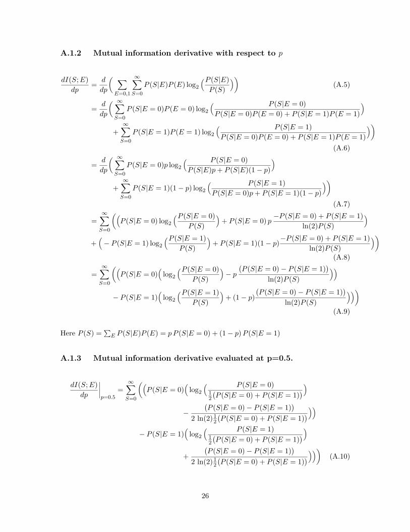
A.1.2 Mutual information derivative with respect to p
dI(S;E)dp
= d
dp
( ∑E=0,1
∞∑S=0
P (S|E)P (E) log2
(P (S|E)P (S)
))(A.5)
= d
dp
( ∞∑S=0
P (S|E = 0)P (E = 0) log2
( P (S|E = 0)P (S|E = 0)P (E = 0) + P (S|E = 1)P (E = 1)
)+∞∑S=0
P (S|E = 1)P (E = 1) log2
( P (S|E = 1)P (S|E = 0)P (E = 0) + P (S|E = 1)P (E = 1)
))(A.6)
= d
dp
( ∞∑S=0
P (S|E = 0)p log2
( P (S|E = 0)P (S|E)p+ P (S|E)(1− p)
)+∞∑S=0
P (S|E = 1)(1− p) log2
( P (S|E = 1)P (S|E = 0)p+ P (S|E = 1)(1− p)
))(A.7)
=∞∑S=0
((P (S|E = 0) log2
(P (S|E = 0)P (S)
)+ P (S|E = 0) p −P (S|E = 0) + P (S|E = 1)
ln(2)P (S))
+(− P (S|E = 1) log2
(P (S|E = 1)P (S)
)+ P (S|E = 1)(1− p)−P (S|E = 0) + P (S|E = 1)
ln(2)P (S)))
(A.8)
=∞∑S=0
((P (S|E = 0)
(log2
(P (S|E = 0)P (S)
)− p
(P (S|E = 0)− P (S|E = 1)
)ln(2)P (S)
))− P (S|E = 1)
(log2
(P (S|E = 1)P (S)
)+ (1− p)
(P (S|E = 0)− P (S|E = 1)
)ln(2)P (S)
)))(A.9)
Here P (S) =∑E P (S|E)P (E) = pP (S|E = 0) + (1− p)P (S|E = 1)
A.1.3 Mutual information derivative evaluated at p=0.5.
dI(S;E)dp
∣∣∣∣p=0.5
=∞∑S=0
((P (S|E = 0)
(log2
( P (S|E = 0)12(P (S|E = 0) + P (S|E = 1)
))−
(P (S|E = 0)− P (S|E = 1)
)2 ln(2)1
2(P (S|E = 0) + P (S|E = 1)
)))− P (S|E = 1)
(log2
( P (S|E = 1)12(P (S|E = 0) + P (S|E = 1)
))+
(P (S|E = 0)− P (S|E = 1)
)2 ln(2)1
2(P (S|E = 0) + P (S|E = 1)
)))) (A.10)
26

For simplicity, take the inner product of the summation and let x = P (S|E = 0) andy = P (S|E = 1)
(P (S|E = 0)
(log2
( P (S|E = 0)12(P (S|E = 0) + P (S|E = 1)
))− (P (S|E = 0)− P (S|E = 1)
)2 ln(2)1
2(P (S|E = 0) + P (S|E = 1)
)))− P (S|E = 1)
(log2
( P (S|E = 1)12(P (S|E = 0) + P (S|E = 1)
))+(P (S|E = 0)− P (S|E = 1)
)2 ln(2)1
2(P (S|E = 0) + P (S|E = 1)
)))(A.11)
= x (log22x
(x+ y) −x− y
ln(2)(x+ y))− y (log22 y
(x+ y) + x− yln(2)(x+ y)) (A.12)
= x (log2 2 + log2 x− log2(x+ y))− (x2 − xy)ln(2)(x+ y) − y (log2 2 + log2 y − log2(x+ y))− (xy − y2)
ln(2)(x+ y)(A.13)
= (x− y)− (x− y) log2(x+ y) + x log2 x− y log2 y −(x2 − y2)
ln(2)(x+ y) (A.14)
= −(x− y) log2(x+ y) + x log2 x− y log2 y + (x− y)− (x− y)ln(2) (A.15)
= −(x− y) log2(x+ y) + x log2 x− y log2 y +(1− 1
ln(2))(x− y) (A.16)
Substituting back into product summation and re-writing in the terms of P (S|E = 0)and P (S|E = 1). The eq. A.17 represents simplified version of derivative of the mutualinformation evaluated at p =0.5.
dI(S;E)dp
∣∣∣∣p=0.5
=∞∑S=0
(−(P (S|E = 0)− P (S|E = 1)
)log2
(P (S|E = 0) + P (S|E = 1)
)+ P (S|E = 0) log2
(P (S|E = 0)
)− P (S|E = 1) log2
(P (S|E = 1)
)+(1− 1
ln(2))(P (S|E = 0)− P (S|E = 1)
))(A.17)
A.2 Derivative of the Mutual information with respect toenvironmental probability plots
A.2.1 Negative binomial distribution
Using the eq. A.17 the results are generated with a particular pair of means, in Fig. A.1and Fig. A.2. Both illustrate the derivative of the mutual information with maximum valuePmax around the environment at Penv = 0.5.
27

0.0 0.2 0.4 0.6 0.8 1.0Penv
4
2
0
2
4
dI(S
;E)
dP(E
)[A][A][A][A][A] b= 5
b= 10b= 20b= 40b= 100
0.0 0.2 0.4 0.6 0.8 1.0Penv
4
2
0
2
4 [B][B][B][B][B] b= 5b= 10b= 20b= 40b= 100
Figure A.1: Derivative of mutual information applied to negative binomial distribution as afunction of environmental probability. [A] Derivative evaluated with mean of pair of µ1 =1, µ2 =17. [B] Derivative evaluated with mean of pair of µ1 =17, µ2 =1. Different burstyparameter b evaluated for derivative of mutual information.
0 20 40 60 80 100b (bursty parameter)
0.10
0.05
0.00
0.05
0.10
dI dP| p
=0.
5
1=1 2=31=1 2=51=1 2=91=1 2=171=1 2=33
0 20 40 60 80 100b (bursty parameter)
0.10
0.05
0.00
0.05
0.101=3 2=11=5 2=11=9 2=11=17 2=11=33 2=1
Figure A.2: Derivative of mutual information applied to negative binomial distributionevaluated at p=0.5 as a function of as a function of bursty parameter for single pair ofmean values.
28