bayesian reference analysis of cointegration 1. introduction many macroeconomic

BAYESIAN REFERENCE ANALYSIS OF COINTEGRATION

MATTIAS VILLANI

Abstract. A Bayesian reference analysis of the cointegrated vector autoregression ispresented based on a new prior distribution. Among other properties, it is shown thatthis prior distribution distributes its probability mass uniformly over all cointegrationspaces for a given cointegration rank. A simple procedure based on the Gibbs sam-pler is used to obtain the posterior distribution of both the number of cointegratingrelations and the form of those relations, together with accompanying error correctingdynamics. Simulated data are used for illustration and for discussing the well-knownissue of local non-identification.

1. Introduction

Many macroeconomic time series behave in a random walk-like fashion and tend tomove around wildly. Typically, such variables move around together, striving to fulfillone or several economic laws, or long run equilibria, which tie them together. A randomwalk is often referred to as an integrated process, and integrated processes that movearound together have therefore been termed cointegrated(Engle and Granger, 1987).

The present work is concerned with estimation of both the number of equilibria, theso called cointegration rank, and the form of the equilibria conditional on the rank.Inferences regarding the error correcting coefficients and other short run dynamics arealso treated.

Several non-Bayesian statistical treatments of cointegration have been presented dur-ing the last two decades, see e.g. Ahn and Reinsel (1990), Phillips (1991) and Stock andWatson (1988). The likelihood-based approach of Søren Johansen is the most widelyused procedure, however; see e.g. Johansen (1991) or Johansen (1995) for a textbooktreatment.

More recently, a handful Bayesian analyses of cointegration have been presented, seeBauwens and Giot (1998), Bauwens and Lubrano (1996), Geweke (1996), Kleibergenand Paap (1998), Kleibergen and van Dijk (1994), Strachan (2000) and Villani (2000).Philosophical issues aside, a Bayesian approach is advantageous for many reasons, e.g.it produces whole probability distributions for each unknown parameter which are validfor any sample size, it affords a straight-forward handling of the inferences for thecointegration rank and tests of restrictions on the model parameters (Geweke, 1996;Kleibergen and Paap, 1998; Strachan, 2000; Villani, 2000), and it makes a satisfactorytreatment of the prediction problem possible (Villani, 2001b).

The crucial step in a Bayesian analysis is the choice of prior distribution and in eachof the above mentioned papers a new prior distribution has been introduced. The degreeof motivation of the priors has varied, but the authors seem to have been more or less

Key words and phrases. Cointegration, Bayesian inference, Estimation, Rank.The author thanks Luc Bauwens, Daniel Thorburn and Herman van Dijk for helpful discussions.

Financial support from the Swedish Council of Research in Humanities and Social Sciences (HSFR) isgratefully acknowledged.

1

2 MATTIAS VILLANI

focused on vague priors which add only a small amount of information into the analysis,i.e. priors largely dominated by data.

This paper will be less concerned with whether or not the prior is ’non-informative’.The aim here is to propose a Bayesian analysis based on a sound prior which appealsto practitioners. Such a prior must consider several partially conflicting aspects ofactual econometric practise: Firstly, the number of parameters in cointegration modelsis usually very large and it is not realistic to demand a detailed subjective specificationof priors on such high-dimensional spaces, at least not at the current state of elicitationtechniques for multivariate distributions. A prior with relatively few hyperparameters,each with a clear interpretation, is thus mandatory. Secondly, priors will not, or atleast should not, be used by practitioners unless they are transparent in the sense thatone can easily understand the kind of information they convey. Thirdly, the prior mustlead to straight-forward posterior calculations which can be performed on a routinebasis without necessary fine tuning in each new application. Finally, the posteriordistribution of the cointegration rank can only be obtained if some parameter matricesare given proper, integrable, priors. A prior which fulfills these objectives will probablynot coincide with the investigators actual prior beliefs, but should nevertheless be usefulas point of reference, or an agreed standard, and is called a reference prior accordingly.

2. The model

Let xtTt=1 be a vector-valued process with p components. The most widely used

model for non-stationary time series is the Error Correction (EC) model

(2.1) ∆xt = Πxt−1 +k−1∑i=1

Γi∆xt−i + Φdt + εt,

where ∆xt−i = xt−i − xt−i−1, Π (p × p) is the matrix of long-run multipliers and Γi

(p× p), for i = 1, ..., k− 1, govern the short run dynamics of the process. dt (w× 1) is avector of trend, seasonal dummies or other exogenous variables with coefficient matrixΦ (p × w). εt (p × 1) contains the unexplained errors at time t which are assumed tofollow the Np(0,Σ) distribution with independence across time periods. The number oflagged differences, k − 1, will be assumed known or determined before the analysis, seeVillani (2001a) for a Bayesian approach.

The stochastic part of a process is integrated of order zero, denoted xt ∼ I(0), if it isstationary while its cumulative sum is not (see Johansen, 1995, p.35 for a more precisedefinition). Furthermore, xt ∼ I(h) if ∆hxt ∼ I(0), i. e. xt is integrated of order h if thehth difference of the process is integrated of order zero.

Even if all p time series in xt are I(1), it can be shown that the condition rank(Π) =r < p implies that r linear combinations of the time series are stationary, see Engle andGranger (1987) and Johansen (1995, p.49); the time series are then cointegrated. Coin-tegration is thus equivalent to the existence of r long run equilibria between otherwisedrifting series. If rank(Π) = r, then Π can be written as a product of two p× r full rankmatrices α and β, and the model in (2.1) can be written

(2.2) ∆xt = αβ′xt−1 +k−1∑i=1

Γi∆xt−i + Φdt + εt,

BAYESIAN COINTEGRATION 3

where β′xt−1 − E(β′xt−1) are the deviations from the r equilibria and α contains theadjustment coefficients governing the dynamics back to equilibrium after a disturbance.The ith column of β contains the coefficients of the ith equilibrium and is called acointegration vector accordingly.

It is well known that only the space spanned by the cointegration vectors (sp β),the cointegration space, is identified, i.e. β is only determined up to arbitrary linearcombinations of its columns. We will follow the traditional route in Bayesian analysesof cointegration by using a linear normalization

(2.3) β =(

Ir

B

)to settle this indeterminacy, where B is a (p−r)×r matrix of fully identified parameters.When β is used as an argument in density functions it must remembered that some ofits elements are known with probability one as a result of the normalization.

The linear normalization is very convenient for computational reasons (see Sections4 and 5) but has the limitation that the existence of B depends on the invertibility ofthe matrix formed by the r first rows in β. Put differently, the linear normalizationimplicitly assumes that each of the r first components of xt enter at least one of the rcointegrating relations, see Strachan (2000) for a thorough discussion.

The linear normalization may blur the interpretation of the estimated cointegrationvectors, but this is easily remedied by a simple transformation of the posterior results,see Section 4.

3. The prior distribution

The prior distribution is conveniently decomposed as

p(α, β, Γ,Σ, r) = p(α, β, Γ,Σ|r)p(r),

where p(r) is any probability distribution over the possible cointegration ranks, r =0,1, ..., p.

The essential conceptual difficulty in a Bayesian approach to cointegration is the priordistribution of α and β. Early contributions include Kleibergen and van Dijk (1994) whosuggested the Jeffreys prior, Bauwens and Lubrano (1996) with a uniform prior on αand student t priors on the cointegration vectors and Geweke’s (1996) normal shrinkagepriors. The Jeffreys prior is complicated, student t priors are used for convenience in theposterior calculation and the normal shrinkage prior is used to assure the convergenceof the algorithm for evaluating the posterior distribution.

Recently, Kleibergen and Paap (1998) proposed a reference prior on α and β which isessentially a prior on Π in the full rank EC model projected down to the subspace whererank(Π) = r; Strachan (2000) extended this idea to more general identifying restrictions.It is an approach which is rather common and well understood in linear models, but itsimplications in non-linear models, such as the EC model with reduced rank in (2.2), arenot as transparent, see also Section 6.

The approach taken here differs from the above mentioned works by focusing directlyon the structure of the parameter space of β, which is non-standard as a result of theidentification problem pointed out in Section 2. We introduce the proposed referenceprior now and spend the rest of this section motivating its particular form. Let Γ =(Γ1, ...,Γk−1,Φ)′ and etr(H) = exp(−1

2 trH), for any square matrix H. The prior canthen be written

4 MATTIAS VILLANI

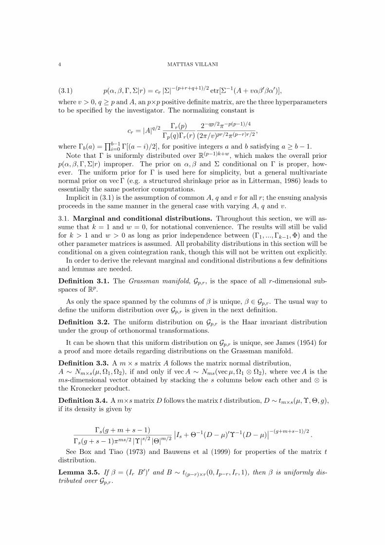
(3.1) p(α, β, Γ,Σ|r) = cr |Σ|−(p+r+q+1)/2 etr[Σ−1(A + vαβ′βα′)],

where v > 0, q ≥ p and A, an p×p positive definite matrix, are the three hyperparametersto be specified by the investigator. The normalizing constant is

cr = |A|q/2 Γr(p)Γp(q)Γr(r)

2−qp/2π−p(p−1)/4

(2π/v)pr/2π(p−r)r/2,

where Γb(a) =∏b−1

i=0 Γ[(a− i)/2], for positive integers a and b satisfying a ≥ b− 1.Note that Γ is uniformly distributed over R(p−1)k+w, which makes the overall prior

p(α, β, Γ,Σ|r) improper. The prior on α, β and Σ conditional on Γ is proper, how-ever. The uniform prior for Γ is used here for simplicity, but a general multivariatenormal prior on vec Γ (e.g. a structured shrinkage prior as in Litterman, 1986) leads toessentially the same posterior computations.

Implicit in (3.1) is the assumption of common A, q and v for all r; the ensuing analysisproceeds in the same manner in the general case with varying A, q and v.

3.1. Marginal and conditional distributions. Throughout this section, we will as-sume that k = 1 and w = 0, for notational convenience. The results will still be validfor k > 1 and w > 0 as long as prior independence between (Γ1, ...,Γk−1,Φ) and theother parameter matrices is assumed. All probability distributions in this section will beconditional on a given cointegration rank, though this will not be written out explicitly.

In order to derive the relevant marginal and conditional distributions a few definitionsand lemmas are needed.

Definition 3.1. The Grassman manifold, Gp,r, is the space of all r-dimensional sub-spaces of Rp.

As only the space spanned by the columns of β is unique, β ∈ Gp,r. The usual way todefine the uniform distribution over Gp,r is given in the next definition.

Definition 3.2. The uniform distribution on Gp,r is the Haar invariant distributionunder the group of orthonormal transformations.

It can be shown that this uniform distribution on Gp,r is unique, see James (1954) fora proof and more details regarding distributions on the Grassman manifold.

Definition 3.3. A m× s matrix A follows the matrix normal distribution,A ∼ Nm×s(µ,Ω1,Ω2), if and only if vec A ∼ Nms(vec µ,Ω1 ⊗ Ω2), where vec A is thems-dimensional vector obtained by stacking the s columns below each other and ⊗ isthe Kronecker product.

Definition 3.4. A m×s matrix D follows the matrix t distribution, D ∼ tm×s(µ,Υ,Θ, g),if its density is given by

Γs(g + m + s− 1)

Γs(g + s− 1)πms/2 |Υ|s/2 |Θ|m/2

∣∣Is + Θ−1(D − µ)′Υ−1(D − µ)∣∣−(g+m+s−1)/2

.

See Box and Tiao (1973) and Bauwens et al (1999) for properties of the matrix tdistribution.

Lemma 3.5. If β = (Ir B′)′ and B ∼ t(p−r)×r(0, Ip−r, Ir, 1), then β is uniformly dis-tributed over Gp,r.


Proof. See Villani (2000).

With the preceding definitions and lemmas out of the way, we are now prepared tostate an important characterization of the distribution in (3.1).

Theorem 3.6. β is marginally uniformly distributed over Gp,r.

Proof. See the appendix.

Thus, the prior in (3.1) assigns equal probability to every possible cointegration spaceof dimension r. This should be a sensible reference prior given that only the cointegrationspace is identified.

Theorem 3.7. The marginal prior of Σ is

Σ ∼ IW (A, q),

where IW denotes the inverted Wishart distribution (Zellner, 1971).

Proof. Follows directly from the proof of Theorem 3.6.

It is easily shown that (see the proof of Theorem 3.8 below)

(3.2) α|β, Σ ∼ Np×r[0, (β′β)−1, v−1Σ].

The linear normalization of β makes α difficult to interpret, however, and the conditionalprior in (3.2) may not shed much light on the prior in (3.1). Consider instead the priorof α conditional on β and Σ when β is orthonormal. Restricting β to be orthonormalis not sufficient to identify the model, however, as any orthonormal version of β can berotated to a new one by postmultiplying it with an r×r orthonormal matrix. This neednot concerns us here as β only enters p(α|β, Σ) in the form β′β and p(α|β, Σ) is thereforeinvariant under these rotations. Define β = β(β′β)−1/2 and note that β is orthonormal.In order for Π = αβ′ to remain unchanged by the transformation β → β, we must makethe corresponding transformation of the adjustment matrix from α to α = α(β′β)1/2.In the following theorem, let αi denote the ith column of α and note that αi describeshow the p response variables are affected by the ith cointegrating relation under theorthonormal normalization.

Theorem 3.8. αi|Σiid∼ Np(0, v−1Σ), i = 1, 2, ..., r.


The rather restrictive form of the prior in Theorem 3.8 must be motivated. First,the restriction to conditional normal priors on α (and thereby also on α) is necessaryfor an efficient numerical evaluation of the posterior based on Gibbs sampling, see Sec-tion 4. Second, non-identical priors on the columns of α do not make sense unlessover-identifying restrictions on the columns of β are used to give a unique meaning toeach cointegration vector, i.e. it is not reasonable to express different beliefs about thecolumns of α without knowing which cointegration vector each αi refers to. Anotherway to see this is that within the class of matrix normal priors α|β, Σ ∼ Np×r(µ,Ω1,Ω2),only the priors with µ = 0, Ω1 = Ir are invariant to rotations of β. Third, the reasonfor centering the conditional prior over zero is motivated by the invariance requirementjust stated. It has the effect of centering the prior over Π = 0, which is often a goodstarting point in an analysis, see the discussion of the ’sum of coefficients’ prior in Doanet al (1984) and the section on prior stability below. Finally, the scale matrix in the con-ditional prior could be any positive definite matrix, the posterior computations remain

6 MATTIAS VILLANI

almost exactly the same. By making the conditional covariance matrix proportional to Σwe incorporate the belief that the uncertainty of a variables error-correcting coefficientsis proportional to size of the unexplained component of that variable.

Further clarification of the hyperparameters A, q and v is obtained from the marginalprior of α. By multiplying p(α|Σ) with the marginal inverted Wishart prior of Σ andintegrating with respect to Σ we obtain

α ∼ tp×r(0, v−1A, Ir, q − p + 1).Results in Box and Tiao (1973, p. 446-7) then give

E(α) = 0 and Cov(vec α) = Ir ⊗ v−1E(Σ),where E(Σ) = A/(q − p− 1) is the expected value of Σ a priori, see e.g. Bauwens et al(1999, p. 306).

A is determined from E(Σ) and q and the investigator thus faces subjective speci-fication of: 1) the expected value of Σ, 2) the degree of certainty regarding Σ (largevalues of q imply large certainty) and 3) the tightness around the point zero for α (largevalues of v give high concentration of probability mass around zero). Note that whethera value for v is large or not depends on E(Σ), which should therefore be specified beforev.

The main difficulty for the investigator is likely to be the specification of E(Σ). Ifinterest only centers on the posterior of α, β, Γ,Σ conditional on a given cointegrationrank, then A may be set equal to the zero matrix and q = 0. This corresponds tousing the usual improper prior p(Σ) ∝ |Σ|−(p+1)/2. If we also aim at analyzing thecointegration rank, but are either unable or unwilling to state our beliefs about Σ, thenA = Σ and q = p + 2 may be used, where Σ is the ML estimate of Σ in the fullrank model; note that this implies that E(Σ) = Σ. This suggestion is of course not aproper Bayesian solution as the prior then becomes dependent on the observed data.The consequences of this side-step are minimized by the choice of the smallest possibleq (maximum uncertainty) subject to a finite expected value of Σ.

3.2. Invariance. The choice of normalizing variables may be somewhat arbitrary andit is therefore desirable to have a posterior distribution which is invariant to this choice.The likelihood function is well-known to have this property and the posterior distributionis therefore invariant if and only if the prior distribution is. Let N1 = i1, ..., ir denotethe set of indices for the r variables used to normalize β. Consider the change innormalization N1 → N2, where N2 equals N1 with jth variable in the normalized setreplaced by the kth variable in the non-normalized set. This change in normalizingvariables is accomplished by the transformation (α, β, Σ) → (α, β, Σ), where α = αU ′,β = βU−1 and U is an r× r transformation matrix whose elements are functions of thekth row of B. The exact form of U need not concern us for the moment, it is sufficientto note that such a matrix always exist if the variables in the new normalizing set enterat least one of the cointegration vectors (see Section 2) and that U then is unique. It isimportant to note that Π = αβ′ is unchanged by the transformation.

The next definition formalizes the idea that the prior distribution (and therefore alsothe posterior distribution) should be the same whether we i) work directly with N1 orii) start with N2 and then transform to N1.


Definition 3.9. A distribution on α, β and Σ is normalization invariant if, for any Ucorresponding to a change in normalizing variables,

p(α, β, Σ) = p(α, β, Σ)J(α, β, Σ → α, β, Σ),where α = αU ′, β = βU−1 and J(α, β, Σ → α, β, Σ) is the Jacobian of the transforma-tion from α, β, Σ to α, β, Σ.

Lemma 3.10. J(α, β, Σ → α, β, Σ) = 1.


Theorem 3.11. The prior in (3.1) is normalization invariant.

Proof.

p(α, β, Σ) = cr |Σ|−(p+r+q+1)/2 etr[Σ−1(A + vαU ′U−1′β′βU−1Uα′)]= p(α, β, Σ),

which, using Lemma 3.10, proves the theorem.

3.3. Prior stability. Define

ΠC =

Ip + αβ′ + Γ1 Γ2 − Γ1 · · · Γk−1 − Γk−2 −Γk−1

Ip 0 · · · 0 00 Ip 0 0...

. . ....

...0 0 · · · Ip 0

The assumption of rank(Π) = r implies that r of the eigenvalues of ΠC are equal to

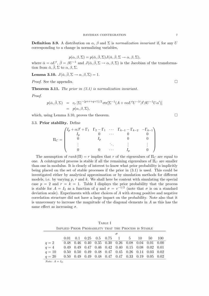
one. A cointegrated process is stable if all the remaining eigenvalues of ΠC are smallerthan one in modulus. It is clearly of interest to know what prior probability is implicitlybeing placed on the set of stable processes if the prior in (3.1) is used. This could beinvestigated either by analytical approximation or by simulation methods for differentmodels, i.e. by varying p, r and k. We shall here be content with simulating the specialcase p = 2 and r = k = 1. Table I displays the prior probability that the processis stable for A = I2 as a function of q and σ = v−1/2 (note that σ is on a standarddeviation scale). Experiments with other choices of A with strong positive and negativecorrelation structure did not have a large impact on the probability. Note also that itis unnecessary to increase the magnitude of the diagonal elements in A as this has thesame effect as increasing σ.

Table I

Implied Prior Probability that the Process is Stable

σ0.01 0.1 0.25 0.5 0.75 1 5 10 50 100

q = 2 0.48 0.46 0.40 0.35 0.30 0.26 0.08 0.04 0.01 0.00q = 4 0.49 0.49 0.47 0.46 0.42 0.40 0.15 0.08 0.02 0.01q = 10 0.50 0.50 0.49 0.48 0.47 0.45 0.26 0.14 0.03 0.02q = 20 0.50 0.49 0.49 0.48 0.47 0.47 0.33 0.19 0.05 0.02Note: A = I2.

8 MATTIAS VILLANI

INSERT FIGURE HERE

Figure 1. Implied prior distribution on the unrestricted eigenvalue.A = I2 and q = 4.

Densities of the unrestricted eigenvalue (λ) are displayed in Figure 1 for differentvalues of σ. The densities are symmetric around the modal value λ = 1. A non-symmetric density for λ which places more mass to the left of λ = 1 than to theright of this point would perhaps better represent actual beliefs. The gain from a non-symmetric prior is probably less than the loss in computational efficiency in the posteriorcalculations, however.

A crude way to obtain a non-symmetric prior is to simply exclude explosive processes apriori (or ’too explosive’ processes, e.g. with eigenvalues larger than 1.1 in modulus) byrestricting the domain of the prior in (3.1) to the space of α, β and Γ where the process isstable. This is neatly handled in the posterior calculations for a given cointegration rankby simply rejecting the draws from the posterior corresponding to non-stable processes,see Section 4. Note that the latter region will be small if the process actually is stableand data informative, and most draws will then be accepted. The posterior distributionof the rank will require heavier numerical computations, however.

4. The posterior distribution conditional on the rank

4.1. Preliminaries. Let us write the cointegrated EC model (2.2) in the followingcompact form

(4.1) Y = Xβα′ + ZΓ + E,

where Y = (∆xT , ...,∆x1)′, X = (xT−1, ..., x0)′, Z = (∆X−1, ...,∆X−k+1, D), ∆X−i =(∆xT−i, ...,∆x−i+1)′, D = (dT , ..., d1)′, Γ = (Γ1, ...,Γk−1,Φ)′ and E = (εT , ..., ε1)′. D =Y, X,Z will be used as a short hand for the available data and d = (p − 1)k + wdenotes the number of columns in Z. Further, define

(4.2) MH = Im −H(H ′H)−1H ′,

for any m× s matrix H.The following two lemmas will be used in some of the proofs later on.

Lemma 4.1.

p(α, β|D, r) ∝∣∣(Y −Xβα′)′MZ(Y −Xβα′) + A + vαβ′βα′

∣∣−(T+q+r−d)/2.


Lemma 4.2. For any non-singular m× s matrix H∫ ∞

−∞

∣∣A + (H −M)′B(H −M)∣∣−h/2

dH = πms/2 Γs(h−m)Γs(h)

|A|−(h−m)/2 |B|−s/2 ,

where A (s× s) and B (m×m) are positive definite matrices, and M (m× s) is of fullrank.

Proof. The integrand is the kernel of a matrix t and the lemma is proved by using thefact that a density integrates to one.


4.2. Marginal posterior distribution of β. The next result gives the marginal pos-terior of the cointegration vectors.

Theorem 4.3. The marginal posterior distribution of β is

p(β|D, r) ∝ |β′C1β|(T+q−d−p)/2

|β′C2β|(T+q−d)/2,

where C1 = X ′MZX + vIp, C2 = vIp + X ′Q[IT − Z(Z ′QZ)−1Z ′Q]X and Q = IT −Y (A + Y ′Y )−1Y ′.


p(β|D, r) in Theorem 4.3 is thus a ratio of two matrix t kernels and could thereforebe termed a matrix 1-1 poly-t density, see Bauwens et al (1999) for a discussion ofmultivariate poly-t densities. Contrary to the multivariate case, no properties havebeen derived for matrix poly-t densities and Theorem 4.3 is therefore of little practicalinterest, in general.

In the special case r = 1, the posterior distribution of B is a (vector-valued) 1-1poly-t density and it can be been shown (Bauwens and Lubrano, 1996) that p(B|D, r)is integrable but has no finite moments. The non-existence of integer moments is not aconsequence of the prior distribution in (3.1), but rather of the linear normalization ofβ, where each element of B is a ratio with the first element of β in the denominator.

4.3. Conditional posteriors and Gibbs sampling. An alternative route to calculatethe posterior distribution of α, B, Γ and Σ using Gibbs sampling (see e.g. Smith andRoberts, 1993, for a good introduction) was pioneered by Geweke (1996).

The Gibbs sampler is an easily implemented iterative method for generating obser-vations from complex multidimensional densities by sampling from the so called fullconditional posterior distributions. The full conditional posterior distribution of a sub-set of parameters in a model is the posterior distribution of the subset conditional onall other parameters. A frequently encountered situation is that the overall posteriordistribution is too complex to generate samples from while the full conditional posteri-ors are all easily sampled. The Gibbs sampler exploits this fact and produces a samplefrom the posterior by iteratively generating parameter values from the full conditionalposteriors.

The sampled parameter values are not independent, but following can be shown tohold under certain conditions which are satisfied here (Geweke, 1996)

θ(i) d→ p(θ|D),

N−1N∑

i=1

f(θ(i)) a.s.→ Eθ|D[f(θ)],

where θ is a parameter vector of interest, θ(i) is the sampled value of θ at the ith Gibbsiteration, d→ and a.s.→ denote convergence in distribution and convergence almost surely,respectively, and p(θ|D) is the posterior distribution of θ conditional on data D. f(·)is any well-behaved function with finite posterior expectation and Eθ|D(·) denotes theposterior expectation.

Initial values for all parameters are needed to start up the Gibbs sampler. Themaximum likelihood estimates in Johansen (1995) are natural candidates.

10 MATTIAS VILLANI

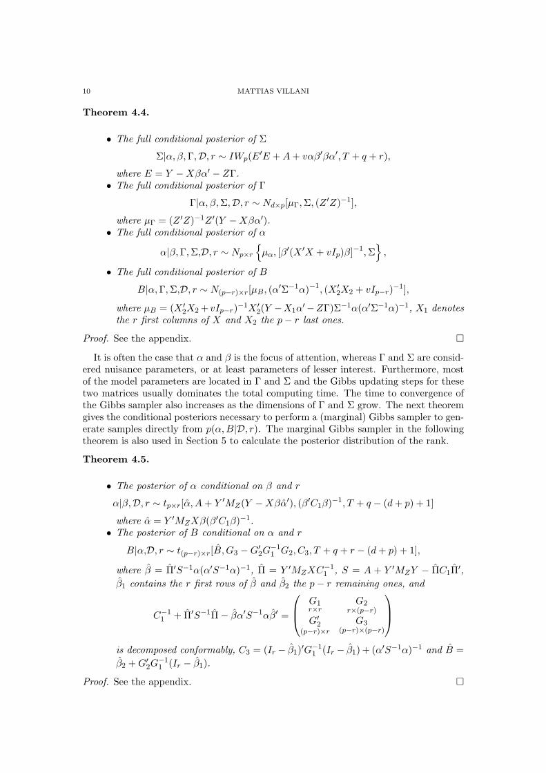
Theorem 4.4.

• The full conditional posterior of Σ

Σ|α, β, Γ,D, r ∼ IWp(E′E + A + vαβ′βα′, T + q + r),

where E = Y −Xβα′ − ZΓ.• The full conditional posterior of Γ

Γ|α, β, Σ,D, r ∼ Nd×p[µΓ,Σ, (Z ′Z)−1],

where µΓ = (Z ′Z)−1Z ′(Y −Xβα′).• The full conditional posterior of α

α|β, Γ,Σ,D, r ∼ Np×r

µα, [β′(X ′X + vIp)β]−1,Σ

,

• The full conditional posterior of B

B|α, Γ,Σ,D, r ∼ N(p−r)×r[µB, (α′Σ−1α)−1, (X ′2X2 + vIp−r)−1],

where µB = (X ′2X2 + vIp−r)−1X ′

2(Y −X1α′−ZΓ)Σ−1α(α′Σ−1α)−1, X1 denotes

the r first columns of X and X2 the p− r last ones.


It is often the case that α and β is the focus of attention, whereas Γ and Σ are consid-ered nuisance parameters, or at least parameters of lesser interest. Furthermore, mostof the model parameters are located in Γ and Σ and the Gibbs updating steps for thesetwo matrices usually dominates the total computing time. The time to convergence ofthe Gibbs sampler also increases as the dimensions of Γ and Σ grow. The next theoremgives the conditional posteriors necessary to perform a (marginal) Gibbs sampler to gen-erate samples directly from p(α, B|D, r). The marginal Gibbs sampler in the followingtheorem is also used in Section 5 to calculate the posterior distribution of the rank.

Theorem 4.5.

• The posterior of α conditional on β and r

α|β,D, r ∼ tp×r[α, A + Y ′MZ(Y −Xβα′), (β′C1β)−1, T + q − (d + p) + 1]

where α = Y ′MZXβ(β′C1β)−1.• The posterior of B conditional on α and r

B|α,D, r ∼ t(p−r)×r[B,G3 −G′2G

−11 G2, C3, T + q + r − (d + p) + 1],

where β = Π′S−1α(α′S−1α)−1, Π = Y ′MZXC−11 , S = A + Y ′MZY − ΠC1Π′,

β1 contains the r first rows of β and β2 the p− r remaining ones, and

C−11 + Π′S−1Π− βα′S−1αβ′ =

G1r×r

G2r×(p−r)

G′2

(p−r)×r

G3(p−r)×(p−r)

is decomposed conformably, C3 = (Ir − β1)′G−1

1 (Ir − β1) + (α′S−1α)−1 and B =β2 + G′

2G−11 (Ir − β1).



The marginal analysis in Theorem 4.5 provides no inferences for Γ and Σ, but theposterior mean and covariance matrix of Γ can be obtained from the marginal Gibbssampler as follows. Note first that

E(Γ|D, r) = Eα,β|D,r[E(Γ|α, β,D, r)](4.3)

C(Γ|D, r) = Eα,β|D,r[C(Γ|α, β,D, r)] + Cα,β|D,r[E(Γ|α, β,D, r)],(4.4)

where Eα,β|D,r and Cα,β|D,r denotes the expectation and covariance with respect to theposterior distribution p(α, B|D, r). By integrating the full posterior distribution withrespect to Σ, it is easily shown that

Γ|α, β,D, r ∼ td×p[µΓ, (Z ′Z)−1,W ′MZW + A + vαβ′βα′, T + q + r − (d + p) + 1],

with µΓ as defined in Theorem 4.4. Thus, using results in Box and Tiao (1973, p. 446-7),we have

E(Γ|α, β,D, r) = µΓ(4.5)

C(Γ|α, β,D, r) =(W ′MZW + A + vαβ′βα′)⊗ (Z ′Z)−1

T + q + r − (d + p + 1).(4.6)

The expectation and covariance with respect to p(α, B|D, r) in (4.3) and (4.4) areeasily computed by averaging the conditional expectation and covariance in (4.5) and(4.6) over the Gibbs samples obtained from the marginal Gibbs sampler in Theorem 4.5.Note that the possibly high-dimensional inverse, (Z ′Z)−1, is fixed in each step of themarginal Gibbs sampler.

It is also straight-forward to show that Σ|α, β,D, r ∼ IW (W ′MZW +A+vαβ′βα′, T +q + r− d). The marginal moments of Σ can be obtained in the same way as for Γ, usingthe expressions for the mean and covariance matrix of the inverted Wishart distribution.

It should be noted, however, that the marginal posteriors of Γ and Σ under reason-ably vague priors seem to be well approximated by the asymptotic distributions of themaximum likelihood estimators of Γ and Σ in Johansen (1995).

We conclude this section with a note on the linear normalization of β. The main ad-vantages of this simple normalization are that the prior which assigns the same probabil-ity to every cointegration space is of rather simple form and that an easily implementedGibbs sampler can be used to compute the posterior results. Note also that we are freeto transform the posterior distribution of α and β as long as the space spanned by thecolumns of β and the matrix of long run multipliers Π = αβ′ remain unchanged, i.e.the class of allowable transformations are (α, β) → (αU ′, βU−1), for any invertible r× rmatrix U . This transformation is conveniently performed directly on the sampled α’sand β’s after the final iteration of the Gibbs sampler. Thus, the restriction to a linearnormalization is in this sense no restriction at all as the final results may be transformedto any desired normalization. The question of existence mentioned in Section 2 is ofcourse still relevant.

12 MATTIAS VILLANI

5. The posterior distribution of the cointegration rank

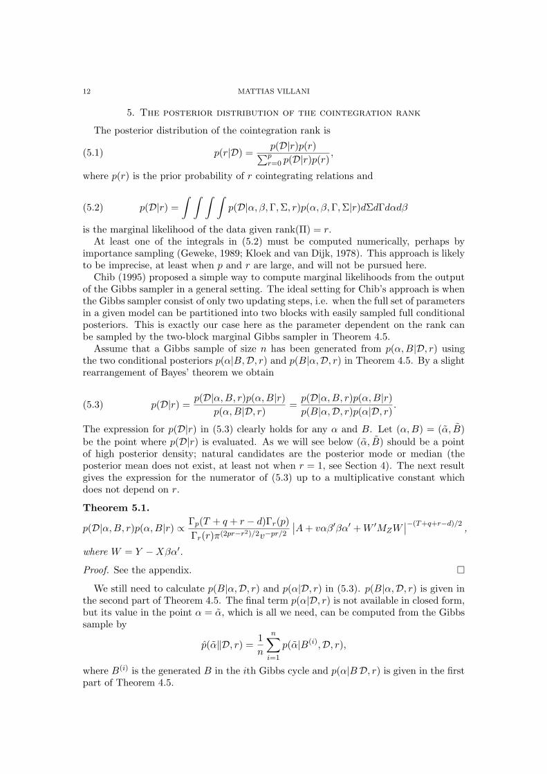
The posterior distribution of the cointegration rank is

(5.1) p(r|D) =p(D|r)p(r)∑p

r=0 p(D|r)p(r),

where p(r) is the prior probability of r cointegrating relations and

(5.2) p(D|r) =∫ ∫ ∫ ∫

p(D|α, β, Γ,Σ, r)p(α, β, Γ,Σ|r)dΣdΓdαdβ

is the marginal likelihood of the data given rank(Π) = r.At least one of the integrals in (5.2) must be computed numerically, perhaps by

importance sampling (Geweke, 1989; Kloek and van Dijk, 1978). This approach is likelyto be imprecise, at least when p and r are large, and will not be pursued here.

Chib (1995) proposed a simple way to compute marginal likelihoods from the outputof the Gibbs sampler in a general setting. The ideal setting for Chib’s approach is whenthe Gibbs sampler consist of only two updating steps, i.e. when the full set of parametersin a given model can be partitioned into two blocks with easily sampled full conditionalposteriors. This is exactly our case here as the parameter dependent on the rank canbe sampled by the two-block marginal Gibbs sampler in Theorem 4.5.

Assume that a Gibbs sample of size n has been generated from p(α, B|D, r) usingthe two conditional posteriors p(α|B,D, r) and p(B|α,D, r) in Theorem 4.5. By a slightrearrangement of Bayes’ theorem we obtain

(5.3) p(D|r) =p(D|α, B, r)p(α, B|r)

p(α, B|D, r)=

p(D|α, B, r)p(α, B|r)p(B|α,D, r)p(α|D, r)

.

The expression for p(D|r) in (5.3) clearly holds for any α and B. Let (α, B) = (α, B)be the point where p(D|r) is evaluated. As we will see below (α, B) should be a pointof high posterior density; natural candidates are the posterior mode or median (theposterior mean does not exist, at least not when r = 1, see Section 4). The next resultgives the expression for the numerator of (5.3) up to a multiplicative constant whichdoes not depend on r.

Theorem 5.1.

p(D|α, B, r)p(α, B|r) ∝ Γp(T + q + r − d)Γr(p)Γr(r)π(2pr−r2)/2v−pr/2

∣∣A + vαβ′βα′ + W ′MZW∣∣−(T+q+r−d)/2 ,

where W = Y −Xβα′.


We still need to calculate p(B|α,D, r) and p(α|D, r) in (5.3). p(B|α,D, r) is given inthe second part of Theorem 4.5. The final term p(α|D, r) is not available in closed form,but its value in the point α = α, which is all we need, can be computed from the Gibbssample by

p(α‖D, r) =1n

n∑i=1

p(α|B(i),D, r),

where B(i) is the generated B in the ith Gibbs cycle and p(α|BD, r) is given in the firstpart of Theorem 4.5.


In order to calculate the marginal likelihoods for r = 0 and r = p, we must choose aprior for the relevant parameter matrices. It is possible to use the prior in (3.1) even inthese extreme cases. This distribution agrees with our earlier prior in the reduced rankcase and has the added benefit of giving tractable integrals. In addition, no new priorhyperparameters needs to be specified by the investigator. If r = 0, then α = β = 0 andthe prior in (3.1) becomes

(5.4) p(Γ,Σ|r) = c0 |Σ|−(p+q+1)/2 etr(Σ−1A),

which is a IW (A, q) prior on Σ and p(Γ) ∝ c. For r = p, Π = αβ′ is of full rank and

(5.5) p(Π,Γ,Σ|r) = cp |Σ|−(2p+q+1)/2 etr[Σ−1(A + vΠΠ′)],

which implies Σ ∼ IW (A, q), vec Π|Σ ∼ Np2(0, Ip ⊗ v−1Σ). The Kronecker structure onthe prior covariance matrix of Π may be too restrictive for some applications, but it ispossible to use a general normal-Wishart prior on Π. Some of the integrals in p(D|r = p)then become intractable, but can be computed from the Gibbs output via Chib’s device,see e.g. Kadiyala and Karlsson (1997) for a simple Gibbs sampler.

The marginal likelihoods for r = 0 and r = p are given in the next theorem.

Theorem 5.2. For the priors in (5.4) and (5.5)

p(D|r = 0) ∝ Γp(T + q − d)∣∣A + Y ′MZY

∣∣−(T+q−d)/2

p(D|r = p) ∝ Γp(T + q − d)vp2/2 |S|−(T+q−d)/2 |C1|−p/2 ,

where S is defined in Theorem 4.5 and C1 is given in Theorem 4.3.


In summary, a complete analysis consist of the following steps:• Generate a sample from each of the p− 1 marginal posteriors p(α, B|D, r), r =

1, 2, ..., p− 1, using the marginal Gibbs sampler in Theorem 4.5 and compute αand B in each sample.

• Compute p(D|r = 0) and p(D|r = p) using the formulas in Theorem 5.2 andp(D|r) for r = 1, 2, ..., p − 1 from the previously generated Gibbs samples asdescribed above. Use (5.1) to compute the posterior distribution of the cointe-gration rank.

• Select the cointegration ranks of interest and summaries the posterior distribu-tion of α and B (possibly transformed to a more interpretable normalization)conditional on these ranks using the already available Gibbs samples.

If inferences about Σ and Γ are wanted for the selected cointegration ranks, and theML estimates with standard errors cannot be used for approximate inference, the fullGibbs sampler in Theorem 4.4 should be used. If the first two posterior moments of Σand Γ are sufficient, the approach based on the marginal Gibbs sampler described inSection 4 is preferred.

Note that p − 1 is typically a rather small number (ranging from 1 to 4 in manyapplications) and that the marginal Gibbs sampler in Theorem 4.5 operates on rathersmall-dimensional spaces, at least compared to the dimension of the whole parameterspace.

14 MATTIAS VILLANI

6. An numerical illustration

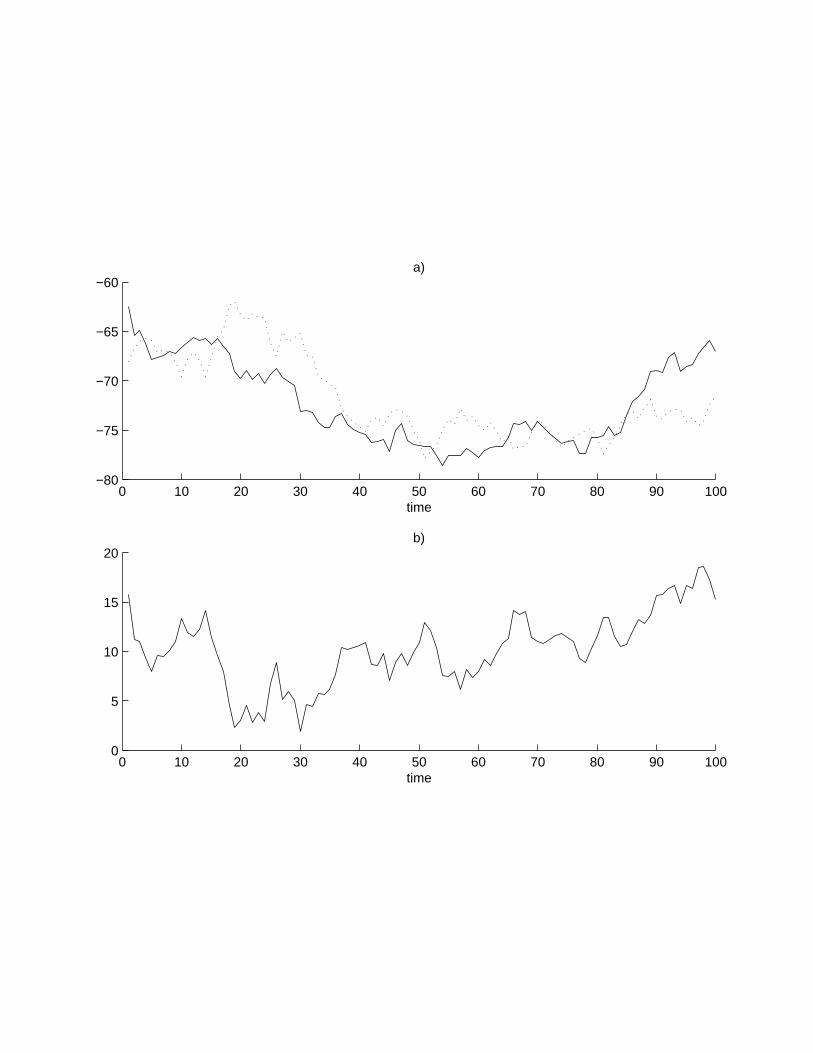
A single data set of length T = 100 was simulated from a bivariate model, withoutshort-run dynamics and constant term, with parameters α = (0, 0.1), β = (1,−1) andΣ = I2. Note that α is close to the zero vector and the model is thus close to thezero rank model. This difficult setup has been chosen in order to accentuate somefeatures of the posterior distribution in cointegration models which were initially raisedby Kleibergen and van Dijk (1994). The simulated time series are displayed in panel a)of Figure 2.

Table II shows the posterior distribution of the cointegration rank for three differentvalues of σ = v−1/2, together with the likelihood trace and maximal eigenvalue tests(Johansen, 1995). A uniform distribution on the ranks was used a priori. q was set to4 and the ML estimate

Σ =(

0.83 -0.10-0.10 1.02,

)

was used for A; other choices of A with larger positive and negative off-diagonal elementshad only minor effects on the results. Note that as Σ ≈ I2, σ corresponds roughly tothe standard deviation of the adjustment coefficients for an orthonormal β, conditionalon Σ, see Theorem 3.8.

The results in Table II are based on 25.000 iterations of the Gibbs sampler (after 1.000burn-in iterations); convergence was reached at a much smaller number of iterations,however. From Table II it is seen that the trace test favors the full rank model whereasthe maximal eigenvalue test prefers r = 0. For the two larger σ, r = 0 has the largestposterior probability. With σ = 0.25, the unit rank model is most probable a posteriori.The inconclusive evidence regarding the cointegration rank is of course expected as wepurposely simulated data from a very difficult parametric setup. Panel b) of Figure 2displays an estimate of the cointegrating relation which does not appear stationary.

It should be noted that the large uncertainty in the rank inference can, and should,be incorporated in the subsequent analysis by averaging these final inferences over theposterior distribution of r.

Table II

Inferences on the cointegration rank

Hypothesis LRtrace LRmax σ = 0.25 σ = 0.5 σ = 1r = 0 17.41∗ 12.43 0.263 0.622 0.874r = 1 4.98∗ 4.98* 0.504 0.337 0.122r = 2 − − 0.233 0.041 0.004

Note: ** and * denotes significant at the 1 and 5 percent level, respectively.

To discuss the issue of local non-identification the simulated data set is analyzedconditional on r = 1. Table III and the first three panels of Figure 3 display theinferences for α1, α2 and B. The striking point in Table III is how insensitive theinferences are to changes in σ; the choice of loss function (which determines the measureof posterior centrality) is more important.


INSERT FIGURE HERE.

Figure 2. a) The two simulated time series. b) Estimated cointegrationrelation, β′xt, with β = (1,−1.15)′.

INSERT FIGURE HERE

Figure 3. The posterior distribution of α and β for σ = 0.5 conditionalon r = 1. θ = arctan(B) is the angle of the cointegration vector inthe orthonormal normalization. 2% of the draws from each tails of theposterior distribution of B were excluded in the histogram construction.

INSERT FIGURE HERE

Figure 4. Sample points from the joint posterior distribution of α andβ for σ = 0.5 conditional on r = 1.

Table III

Posterior distribution of α and β conditional on r = 1

Posterior mode Posterior medianML σ = 0.25 σ = 0.5 σ = 1 σ = 0.25 σ = 0.5 σ = 1

α1 0.016 0.015 0.012 0.015 0.010 0.010 0.011α2 0.096 0.079 0.089 0.091 0.080 0.083 0.083B −1.171 −1.063 −1.061 −1.031 −1.151 −1.137 −1.150Note: All estimates are based on 25.000 Gibbs iterations (excluding burn-in).

The extra local mode in the marginal posterior of α2 = 0 in Figure 3 is an effect ofthe local non-identification discussed in Kleibergen and van Dijk (1994). They pointedout that when α = (0, 0)′, β drops out of the likelihood function and the likelihoodis then constant along the B-axis (which has infinite length) and all values for B areobservationally equivalent; B is said to be locally non-identified when α = (0, 0)′. Theposterior distribution based on the prior in (3.1) has the same property as it is flat inthe direction of B when α is the zero vector. This is illustrated in Figure 4, where thesample points from p(α1, B|D, r = 1) and p(α2, B|D, r = 1) are displayed. Note how theconditional variance of B grows as α → 0. The posterior variance of B given α = 0 isactually infinite as can be seen from the second part of Theorem 4.5. This of course asit should be: if the processes do not react at all to past deviations from the equilibrium,then the data are necessarily uninformative regarding the cointegration vector.

Kleibergen and van Dijk (1994) argue that this local non-identification causes prob-lems for a Bayesian analysis with uniform, improper, priors on α and B. Their argu-ment is as follows: the marginal posterior of α is obtained by integrating the posteriorp(α, B|D) with respect to B. As the posterior under a uniform prior is flat along theB-axis when α = (0, 0)′, the marginal posterior density of α in the point α = (0, 0)′ isproportional to the integral of a constant over an unbounded region (−∞ < B < ∞),i.e. infinity. The marginal posterior of α is thus expected to have an asymptote in thepoint (0, 0)′ which is entirely created by the local non-identification. This conclusion isgiven without formal proof, but a numerical example is used to support the argument.

Kleibergen and van Dijk suggests the Jeffreys prior to counter-attack the unwantedasymptote as this prior is zero in the locally non-identified points. The prior in Kleiber-gen and Paap (1998) has the same property. In the case of unit rank their prior reduces

16 MATTIAS VILLANI

top(α, β) ∝ (‖α‖ ‖β‖)(p−1)/2 ,

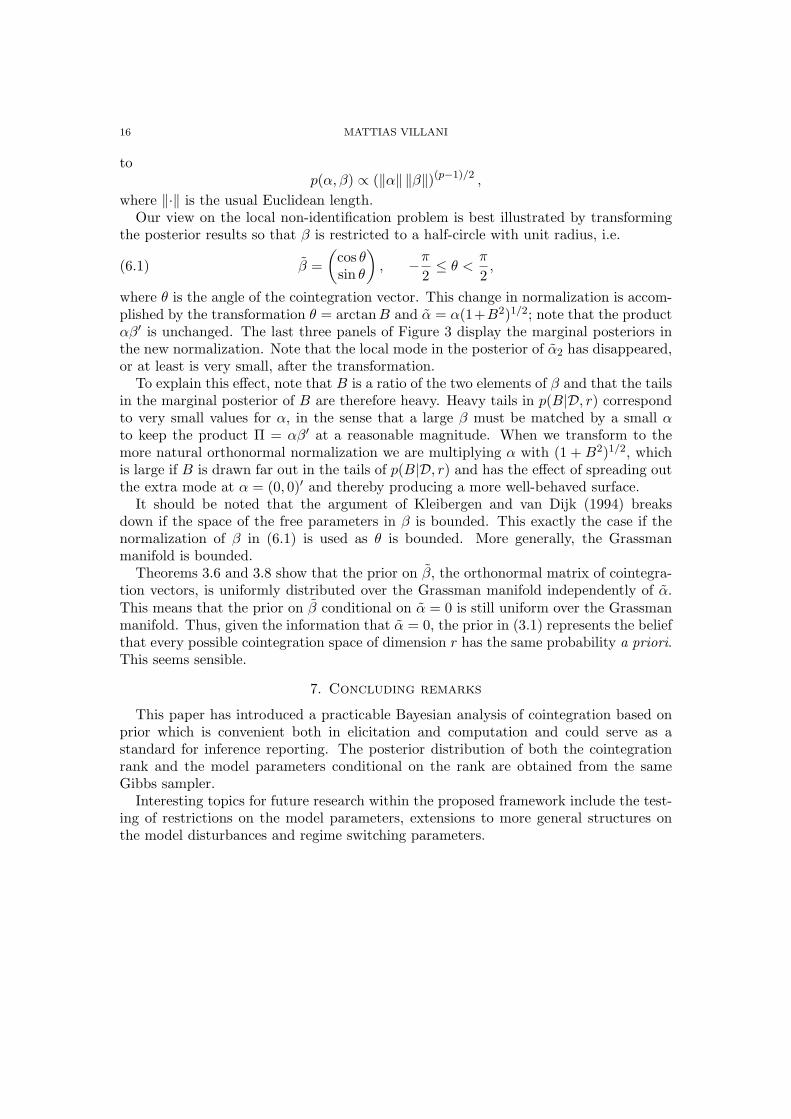
where ‖·‖ is the usual Euclidean length.Our view on the local non-identification problem is best illustrated by transforming

the posterior results so that β is restricted to a half-circle with unit radius, i.e.

(6.1) β =(

cos θsin θ

), −π

2≤ θ <

π

2,

where θ is the angle of the cointegration vector. This change in normalization is accom-plished by the transformation θ = arctanB and α = α(1+B2)1/2; note that the productαβ′ is unchanged. The last three panels of Figure 3 display the marginal posteriors inthe new normalization. Note that the local mode in the posterior of α2 has disappeared,or at least is very small, after the transformation.

To explain this effect, note that B is a ratio of the two elements of β and that the tailsin the marginal posterior of B are therefore heavy. Heavy tails in p(B|D, r) correspondto very small values for α, in the sense that a large β must be matched by a small αto keep the product Π = αβ′ at a reasonable magnitude. When we transform to themore natural orthonormal normalization we are multiplying α with (1 + B2)1/2, whichis large if B is drawn far out in the tails of p(B|D, r) and has the effect of spreading outthe extra mode at α = (0, 0)′ and thereby producing a more well-behaved surface.

It should be noted that the argument of Kleibergen and van Dijk (1994) breaksdown if the space of the free parameters in β is bounded. This exactly the case if thenormalization of β in (6.1) is used as θ is bounded. More generally, the Grassmanmanifold is bounded.

Theorems 3.6 and 3.8 show that the prior on β, the orthonormal matrix of cointegra-tion vectors, is uniformly distributed over the Grassman manifold independently of α.This means that the prior on β conditional on α = 0 is still uniform over the Grassmanmanifold. Thus, given the information that α = 0, the prior in (3.1) represents the beliefthat every possible cointegration space of dimension r has the same probability a priori.This seems sensible.

7. Concluding remarks

This paper has introduced a practicable Bayesian analysis of cointegration based onprior which is convenient both in elicitation and computation and could serve as astandard for inference reporting. The posterior distribution of both the cointegrationrank and the model parameters conditional on the rank are obtained from the sameGibbs sampler.

Interesting topics for future research within the proposed framework include the test-ing of restrictions on the model parameters, extensions to more general structures onthe model disturbances and regime switching parameters.


References

Ahn, S. K. and Reinsel, G. C. (1990). Estimation for partially non-stationary multivariate autoregressiveprocesses, Journal of the American Statistical Association, 85, 813-23.

Bauwens, L. and Giot, P. (1998). A Gibbs sampler approach to cointegration, Computational Statistics,13, 339-68.

Bauwens, L. and Lubrano, M. (1996). Identification restrictions and posterior densities in cointegratedGaussian VAR systems. In Advances in Econometrics, Volume 11, Part B, JAI Press, 3-28.

Bauwens, L., Lubrano, M. and Richard, J.-F. (1999). Bayesian Inference in Dynamic EconometricModels, Oxford: Oxford University Press.

Box, G. E. P. and Tiao, G. C. (1973). Bayesian Inference in Statistical Analysis. Reading, MA: Addison-Wesley.

Chib, S. (1995). Marginal likelihood from the Gibbs output, Journal of the American Statistical Asso-ciation, 90, 1313-21.

Doan, T., Litterman, R. B. and Sims, C. A. (1984). Forecasting and conditional projection usingrealistic prior distributions, Econometrics Reviews, 3, 1-100.

Engle, R. F. and Granger, C. W. J. (1987). Co-integration and error correction: Representation,estimation and testing. Econometrica, 55, 251-76.

Geweke, J. (1989). Bayesian inference in econometric models using Monte Carlo integration, Econo-metrica, 57, 1317-40.

Geweke, J. (1996). Bayesian reduced rank regression in econometrics, Journal of Econometrics, 75,121-46.

Harville, D. A. (1997). Matrix Algebra From a Statistician’s Perspective. New York: Springer-Verlag.

James, A. T. (1954). Normal multivariate analysis and the orthogonal group, Ann. Math. Statist., 25,40-74.

Johansen, S. (1991). Estimation and hypothesis testing of cointegration vectors in Gaussian vectorautoregressive models, Econometrica, 59, 1551-80.

Johansen, S. (1995). Likelihood-Based Inference in Cointegrated Vector Autoregressive Models. Oxford:Oxford University Press.

Kadiyala, K. R. and Karlsson, S. (1997). Numerical methods for estimation and inference in BayesianVAR-models, Journal of Applied Econometrics, 12, 99-132.

Kleibergen, F. and van Dijk, H. K. (1994). On the shape of the likelihood/posterior in cointegrationmodels, Econometric Theory. 10, 514-51.

Kleibergen, F. and Paap, R. (1998). Priors, posterior odds and Lagrange multiplier statistics in Bayesiananalysis of cointegration. Econometric Institute Report, no. 9821/A, Econometric Institute, ErasmusUniversity Rotterdam.

Kloek, T. and van Dijk, H. K. (1978). Bayesian estimates of equation system parameters: an applicationof integration by Monte Carlo, Econometrica, 46, 1-19.

Litterman, R. B. (1986). Forecasting with Bayesian vector autoregressions - Five years of experience,Journal of Business and Economic Statistics. 4, 25-38.

Phillips, P. C. B. (1991). Optimal inference in cointegrated systems, Econometrica, 59, 283-306.

Stock, J. H. and Watson, M. W. (1988). Testing for common trends, Journal of the American StatisticalAssociation, 83, 1097-107.

Strachan, R. W. (2000). Bayesian analysis of the cointegrating error correction model: with extensionto general reduced rank regression models. PhD thesis, Monash University, Australia.

Villani, M. (2000). Aspects of Bayesian Cointegration. PhD thesis, Stockholm University, Sweden.

Villani, M. (2001a). Fractional Bayesian lag length inference in multivariate autoregressive processes,Journal of Time Series Analysis, 22, 67-86.

Villani, M. (2001b). Bayesian Prediction with Cointegrated Vector Autoregressions, International Jour-nal of Forecasting, forthcoming.

Zellner, A. (1971). An Introduction to Bayesian Inference in Econometrics. New York: Wiley.

18 MATTIAS VILLANI

Appendix A. Proofs

A.1. Proof of Theorem 3.6. To obtain the marginal distribution of β, we first derive the marginaldistribution of B. The joint prior of B and Σ is

p(B, Σ) =

∫p(α, B, Σ)dα = cr |Σ|−(p+r+q+1)/2

∫etr[Σ−1(A + vαβ′βα′)]dα

= cr |Σ|−(p+r+q+1)/2 etr(Σ−1A)

∫etr(Σ−1vαβ′βα′)dα.

By Theorem 16.2.2 in Harville

tr(Σ−1vαβ′βα′) = vec(α)′(β′β ⊗ vΣ−1) vec(α).

Thus, using properties of the normal distribution,

p(B, Σ) = cr |Σ|−(p+r+q+1)/2 etr(Σ−1A)

∫exp

−1

2vec(α)′[β′β ⊗ vΣ−1] vec(α)

d vec α

= cr |Σ|−(p+r+q+1)/2 etr(Σ−1A)(2π)pr/2∣∣β′β ⊗ vΣ−1

∣∣−1/2

= cr(2π/v)pr/2 |Σ|−(p+q+1)/2 etr(Σ−1A)∣∣Ir + B′B

∣∣−p/2.

This shows that B and Σ are independent and marginally B ∼ t(p−r)×r(0, Ip−r, Ir, 1). Thus, usingLemma 3.5, β is uniformly distributed over Gp,r.

A.2. Proof of Theorem 3.8. First we derive the distribution of α conditional on β and Σ

p(α|β, Σ) =p(α, β, Σ)

p(β, Σ)=

cr |Σ|−(p+r+q+1)/2 etr[Σ−1(A + vαβ′βα′)]

cr(2π/v)pr/2 |Σ|−(p+q+1)/2 etr(Σ−1A) |Ir + B′B|−p/2

= (2π)−pr/2∣∣(β′β)−1 ⊗ v−1Σ

∣∣−1/2exp

−1

2(vec α)′(β′β ⊗ vΣ−1)(vec α)

.

Thus,

α|β, Σ ∼ Np×r[0, (β′β)−1, v−1Σ].

As α = α(β′β)1/2 we have (see e.g. Bauwens et al 1999, p. 302)

α|β, Σ ∼ Np×r(0, Ir, v−1Σ).

The density p(α|β, Σ) is not a function of β and we may write α|Σ ∼ Np×r(0, Ir, v−1Σ). The statement of

the theorem now follows from the usual independence property of the multivariate normal distribution.

A.3. Proof of Lemma 3.10. Let N1 denote that β is normalized on the r first variables and N2 thatβ is normalized on variables 1, 2, ..., r − 1 and r + 1, i.e. the change in normalizing variables from N1

to N2 is accomplished by replacing the last variable of the normalizing set with the first variable in thenon-normalizing set. It will be evident that the lemma holds generally under any change in normalizingvariables. Let

B =

b1,1 b1,2 · · · b1,r

b2,1 b2,2 · · · b2,r

......

. . ....

bp−r,1 bp−r,2 · · · bp−r,r

,

denote the matrix of free coefficients in β under N1. The transformation matrix in this case is

U =

(J

b1,1, b1,2, ..., b1,r

), if r > 1 and U = b1,1 if r = 1,


where J denotes the r − 1 first rows of Ir. To see that U actually produces the intended change innormalization note that

β =

(Ir

B

)U−1 =

J−b1,1b

−11,r −b1,2b

−11,r · · · b−1

1,r

0 0 · · · 1b2,1 − b2,rb1,1b

−11,r b2,2 − b2,rb1,2b

−11,r · · · b2,rb

−11,r

......

. . ....

bp−r,1 − bp−r,rb1,1b−11,r bp−r,2 − bp−r,2b1,2b

−11,r · · · bp−r,rb

−11,r

as can be verified by direct calculation. It is easy to see that |U | = b1,r and

U−1 =

(J

−b1,1b−11,r,−b1,2b

−11,r, ..., b

−11,r

), if r > 1 and U−1 = b−1

1,1 if r = 1,

The matrix of free coefficients under N2 is

(A.1) B =

−b1,1b

−11,r −b1,2b

−11,r · · · b−1

1,r

b2,1 − b2,rb1,1b−11,r b2,2 − b2,rb1,2b

−11,r · · · b2,rb

−11,r

......

. . ....

bp−r,1 − bp−r,rb1,1b−11,r bp−r,2 − bp−r,rb1,2b

−11,r · · · bp−r,rb

−11,r

.

The change in normalization from N2 to N1 is thus given by the transformation α, B, Σ → α, B, Σ,where α = αU ′. The Jacobian of this transformation is

(A.2) J(α, β, Σ → α, β, Σ) =

∣∣∣∣∣d vec(α)d vec(α)′

d vec(α)d vec(B)′

d vec(B)d vec(α)′

d vec(B)d vec(B)′

∣∣∣∣∣ = |U |p∣∣∣∣ d vec(B)

d vec(B)′

∣∣∣∣ ,

as Σ is unaffected by the transformation, d vec(B)d vec(α)′ = 0 and d vec(α)

d vec(α)′ = U ⊗ Ip. From the definition of thevec-operator,

∣∣∣∣ d vec(B)

d vec(B)′

∣∣∣∣ =

∣∣∣∣∣∣∣∣∣∣

db1db1

db1db2

· · · db1dbr

db2db1

db2db2

· · · db2dbr

......

. . ....

dbrdb1

dbrdb2

· · · dbrdbr

∣∣∣∣∣∣∣∣∣∣,

where bi and bi are the ith column of B and B, respectively. It is easily seen from (A.1) that dbidbj

= 0

for i > j, and thus

(A.3)

∣∣∣∣ d vec(B)

d vec(B)′

∣∣∣∣ =

∣∣∣∣db1

db1

∣∣∣∣ ∣∣∣∣db2

db2

∣∣∣∣ · · · ∣∣∣∣dbr

dbr

∣∣∣∣ ,

where

(A.4)dbi

dbi=

(−b−1

1,r 0· Ip−r−1

), for i = 1, ..., r − 1, and

dbr

dbr=

db1

db1b−11,r,

and the dot replaces an expression which is unnecessary to calculate. Thus, from (A.2), (A.3) and (A.4)

J(α, β, Σ → α, β, Σ) = |U |p∣∣∣∣db1

db1

∣∣∣∣ ∣∣∣∣db2

db2

∣∣∣∣ · · · ∣∣∣∣dbr

dbr

∣∣∣∣ = bp1,r(b

−11,r)

r(b−11,r)

p−r = 1.

A.4. Proof of Lemma 4.1. The joint posterior of α, β, Γ, Σ is

p(α, β, Γ, Σ|D, r) ∝ p(D|α, β, Γ, Σ, r)p(α, β, Γ, Σ|r)∝ |Σ|−(T+p+r+q+1)/2 etr[Σ−1(E′E + A + vαβ′βα′)],

where E = Y −Xβα′ − ZΓ. Using properties of the inverted Wishart density (Zellner, 1971),

p(α, β, Γ|D, r) ∝∣∣E′E + A + vαβ′βα′∣∣−(T+q+r)/2

.

Let W = Y −Xβα′. We have

E′E = (W − ZΓ)′(W − ZΓ) = W ′MZW + (Γ− Γ)′Z′Z(Γ− Γ),

20 MATTIAS VILLANI

where Γ = (Z′Z)−1Z′W . Thus, by Lemma 4.2

p(α, β|D, r) ∝∫ ∣∣∣W ′MZW + A + vαβ′βα′ + (Γ− Γ)′Z′Z(Γ− Γ)

∣∣∣−(T+q+r)/2

dΓ

∝∣∣(Y −Xβα′)′MZ(Y −Xβα′) + A + vαβ′βα′∣∣−(T+q+r−d)/2

.

A.5. Proof of Theorem 4.3. The following proof follows closely the proof of Theorem 3.1 in Bauwensand Lubrano (1996). From the proof of Lemma 4.1

(A.5) p(α, β, Γ|D) ∝∣∣E′E + A + ∆′F∆

∣∣−(T+q+r)/2

where

∆(r+d)×p

=

(α′

Γ

), F =

(vβ′β 0

0 0

)E = Y −W∆ and W = (Xβ, Z). The equality

(A.6) E′E + A + ∆′F∆ = C + (∆− ∆)′(W ′W + F )(∆− ∆),

where ∆ = (W ′W + F )−1W ′Y and C = A + Y ′Y − Y ′W (W ′W + F )−1W ′Y , can be verified by directcalculation. Inserting (A.6) in (A.5) and integrating out ∆ using Lemma 4.2 gives

p(β|D) ∝∫ ∣∣∣C + (∆− ∆)′(W ′W + F )(∆− ∆)

∣∣∣−(T+q+r)/2

d∆

∝ |C|−(T+q−d)/2∣∣W ′W + F

∣∣−p/2.

Using the result ∣∣D4 −D3D−11 D2

∣∣ = |D1|−1 |D4|∣∣D1 −D2D

−14 D3

∣∣ ,

which holds for any conformable matrices D1, D2, D3 and D4, we can write

|C| =∣∣A + Y ′Y − Y ′W (W ′W + F )−1W ′Y

∣∣ =∣∣W ′W + F

∣∣−1 ∣∣A + Y ′Y∣∣ ∣∣F + W ′QW

∣∣ ,

where Q = IT − Y (A + Y ′Y )−1Y ′. Thus,

(A.7) p(β|D) ∝∣∣F + W ′QW

∣∣−(T+q−d)/2 ∣∣W ′W + F∣∣(T+q−d−p)/2

,

where ∣∣W ′W + F∣∣ =

∣∣∣∣ β′(X ′X + vIp)β β′X ′ZZ′Xβ Z′Z

∣∣∣∣=

∣∣Z′Z∣∣ ∣∣β′ vIp + X ′[IT − Z(Z′Z)−1Z′]X

β∣∣ ,(A.8)

and ∣∣F + W ′QW∣∣ =

∣∣∣∣ β′(X ′QX + vIp)β β′X ′QZZ′QXβ Z′QZ

∣∣∣∣=

∣∣Z′QZ∣∣ ∣∣β′ vIp + X ′Q[IT − Z(Z′QZ)−1Z′Q]X

β∣∣ .(A.9)

Inserting (A.8) and (A.9) in (A.7) proves the result.

A.6. Proof of Theorem 4.4. All full conditional posteriors are proportional to the likelihood functionmultiplied with the prior in (3.1), i.e. proportional to

(A.10) |Σ|−(T+p+r+q+1)/2 etr[Σ−1(E′E + A + vαβ′βα′)],

where E = Y −Xβα′ − ZΓ.It follows directly from (A.10) that the full conditional posterior of Σ is the IWp(E′E + A +

vαβ′βα′, T + q + r) density.The full conditional posterior of Γ follows from the treatment of the multivariate regression in Zellner

(1971); see also Geweke (1996).To obtain the full conditional posterior of B, let X = (X1, X2), where X1 contains the r first columns

of X and X2 contains the p−r remaining ones, and W = Y −X1α′−ZΓ. The full conditional likelihood

of B is then


p(D|α, β, Γ, Σ, r) ∝ etr[Σ−1(W −X2Bα′)′(W −X2Bα′)]

= etr[(WΣ−1/2 −X2Bα′Σ−1/2)′(WΣ−1/2 −X2Bα′Σ−1/2)]

= exp

−1

2

[vec(WΣ−1/2)−H vec B

]′ [vec(WΣ−1/2)−H vec B

],

where H = (Σ−1/2α⊗X2). Thus,

(A.11) p(D|α, β, Γ, Σ, r) ∝ exp

−1

2(vec B − vec B)′(α′Σ−1α⊗X ′

2X2)(vec B − vec B)

,

where

vec B =[(α′Σ−1α)−1 ⊗ (X ′

2X2)−1] (α′Σ−1/2 ⊗X ′

2) vec(WΣ−1/2)

= vec[(X ′

2X2)−1X ′

2WΣ−1α(α′Σ−1α)−1] .

The prior in (3.1) can be rewritten as

p(α, B, Σ, Γ|r) ∝ etr(Σ−1vαα′) etr(Σ−1vαB′Bα′)

∝ exp

−1

2(vec B)′(α′Σ−1α⊗ vIp−r)(vec B)

.(A.12)

By multiplying (A.11) by p(α, B, Σ, Γ|r) in (A.12) and completing the square in the exponential (seeLemma 1 in Box and Tiao, 1973, p. 418), it is seen that

p(B|α, Γ, Σ,D, r) ∝ exp

−1

2(vec B − vec µB)′Ω−1

B (vec B − vec µB)

,

where Ω−1B = α′Σ−1α⊗ (X ′

2X2 + vIp−r) and

vec µB = ΩB(α′Σ−1α⊗X ′2X2) vec B = vec[(X ′

2X2 + vIp−r)−1X ′

2WΣ−1α(α′Σ−1α)−1].

Thus, B|α, Γ, Σ, D ∼ N(p−r)×r[µB , (α′Σ−1α)−1, (X ′2X2 + vIp−r)

−1].To derive the full conditional posterior of α, let Q = Y − ZΓ. The full conditional likelihood of α is

p(D|α, β, Γ, Σ, r) ∝ etr[Σ−1(Q−Xβα′)′(Q−Xβα′)]

= etr[(QΣ−1/2 −Xβα′Σ−1/2)′(QΣ−1/2 −Xβα′Σ−1/2)]

∝ exp

−1

2

[vec(α′)− vec(α′)

]′ (Σ−1 ⊗ β′X ′Xβ

) [vec(α′)− vec(α′)

]= exp

−1

2(vec α− vec α)′

(β′X ′Xβ ⊗ Σ−1) (vec α− vec α)

where

vec(α′) =[Σ⊗ (β′X ′Xβ)−1] (Σ−1/2 ⊗ β′X ′) vec(QΣ−1/2)

= vec[(β′X ′Xβ)−1β′X ′Q

].

Thus,

α = Q′Xβ(β′X ′Xβ)−1.

By multiplying the conditional likelihood of α with

p(α, β, Σ, Γ|r) ∝ exp

−1

2(vec α)′(β′β ⊗ vΣ−1)(vec α)

we obtain (see Lemma 1 in Box and Tiao, 1973, p. 418)

p(α|β, Σ, Γ,D, r) ∝ exp

−1

2(vec α− vec µα)′ Ω−1

α (vec α− vec µα)

,

where Ω−1α = β′(X ′X + vIp)β ⊗ Σ−1 and

vec µα = Ωα(β′X ′Xβ ⊗ Σ−1) vec α = vec(Q′Xβ[β′(X ′X + vIp)β]−1) .

22 MATTIAS VILLANI

A.7. Proof of Theorem 4.5. From Lemma 4.1, we have

p(α|β,D, r) ∝∣∣(Y −Xβα′)′MZ(Y −Xβα′) + A + vαβ′βα′∣∣−(T+q+r−d)/2

=∣∣A + Y ′MZ(Y −Xβα′) + (α′ − α′)′(β′C1β)(α′ − α′)

∣∣−(T+q+r−d)/2.

where α′ = (β′C1β)−1β′X ′MZY . Thus, α′ ∼ tr×p[α′, (β′C1β)−1, A+Y ′MZ(Y −Xβα′), T+q−(d+p)+1].From Box and Tiao (1973, p. 442), α ∼ tp×r[α, A + Y ′MZ(Y −Xβα′), (β′C1β)−1, T + q − (d + p) + 1].

Since Π = αβ′, the posterior of β conditional on α can be written

p(β|α,D, r) ∝∣∣(Y −XΠ′)′MZ(Y −XΠ′) + A + vΠΠ′∣∣−(T+q+r−d)/2

=∣∣∣S + (Π− Π)C1(Π− Π)′

∣∣∣−(T+q+r−d)/2

,

where S = A + Y ′MZY − ΠC1Π′ and Π = Y ′MZXC−1

1 . Thus,

p(β|α,D, r) ∝∣∣∣C−1

1 + (αβ′ − Π)′S−1(αβ′ − Π)∣∣∣−(T+q+r−d)/2

=∣∣∣R + (β − β)(α′S−1α)(β − β)′

∣∣∣−(T+q+r−d)/2

∝∣∣∣(α′S−1α)−1 + (β − β)′R−1(β − β)

∣∣∣−(T+q+r−d)/2

(A.13)

where β = Π′S−1α(α′S−1α)−1 and R = C−11 + Π′S−1Π − β(α′S−1α)β′. Let β = (β′1, β

′2)′, where β1

contains the r first rows of β and β2 the p− r remaining ones, and R is conformably decomposed as

R =

G1r×r

G2r×(p−r)

G′2

(p−r)×r

G3(p−r)×(p−r)

By using the result (see e.g. Harville, 1997)

R−1 =

((G1 −G2G

−13 G′

2)−1 −(G1 −G2G

−13 G′

2)−1G2G

−13

−G−13 G′

2(G1 −G2G−13 G′

2)−1 (G3 −G′

2G−11 G2)

−1

)it is straight-forward to show that

(β − β)′R−1(β − β) = (Ir − β1)′G−1

1 (Ir − β1) + (B − B)′(G3 −G′2G

−11 G2)

−1(B − B),

where B = β2 + G′2G1(Ir − β1). From (A.13)

p(B|α,D, r) ∝∣∣∣C3 + (B − B)′(G3 −G′

2G−11 G2)

−1(B − B)∣∣∣−(T+q+r−d)/2

,

where C3 = (Ir−β1)′G−1

1 (Ir−β1)+(α′S−1α)−1. This is proportional to the matrix t density in Theorem4.5.

A.8. Proof of Theorem 5.1. Using properties of the inverted Wishart density,

(A.14) p(α, B|r) =

∫p(α, B, Σ|r)dΣ = cr2

p(q+r)/2πp(p−1)/4Γp(q + r)∣∣A + vαβ′βα′∣∣−(q+r)/2

.

(A.15) p(D|α, B, r) =

∫∫p(D|α, B, Γ, Σ, r)p(Γ, Σ|α, B, r)dΣdΓ,

where

p(Γ, Σ|α, B, r) =p(α, B, Γ, Σ|r)

p(α, B|r) =|Σ|−(p+r+q+1)/2 etr[Σ−1(A + vαβ′βα′)]

2p(q+r)/2πp(p−1)/4Γp(q + r) |A + vαβ′βα′|−(q+r)/2.

Thus, from (A.15)

p(D|α, B, r) =

∫∫(2π)−Tp/2 |Σ|−T/2 etr(Σ−1E′E)

|Σ|−(p+r+q+1)/2 etr[Σ−1(A + vαβ′βα′)]

2p(q+r)/2πp(p−1)/4Γp(q + r) |A + vαβ′βα′|−(q+r)/2dΣdΓ

= k1

∫ ∣∣E′E + A + vαβ′βα′∣∣−(T+q+r)/2dΓ,

where k1 = π−Tp/2 |A + vαβ′βα′|(q+r)/2Γp(T + q + r)/Γp(q + r). Let W = Y −Xβα′. We have

E′E = (W − ZΓ)′(W − ZΓ) = W ′MZW + (Γ− Γ)′Z′Z(Γ− Γ),


where Γ = (Z′Z)−1Z′W . Thus, using Lemma 4.2

p(D|α, B, r) = k1

∫ ∣∣∣A + vαβ′βα′ + W ′MZW + (Γ− Γ)′Z′Z(Γ− Γ)∣∣∣−(T+q+r)/2

dΓ

= k1πpd/2 Γp(T + q + r − d)

Γp(T + q + r)

∣∣A + vαβ′βα′ + W ′MZW∣∣−(T+q+r−d)/2 ∣∣Z′Z

∣∣−p/2.

Multiplying p(D|α, B, r) with p(α, B|r) and simplifying gives

p(D|α, B, r)p(α, B|r) = k2Γr(p)Γp(T + q + r − d)

Γr(r)π(2pr−r2)/2v−pr/2

∣∣A + vαβ′βα′ + W ′MZW∣∣−(T+q+r−d)/2

,

where k2 =|Z′Z|−p/2|A|q/2

πp(T−d)/2Γp(q)also appears in the marginal likelihood of r = 0 and r = p (see the proof of

Theorem 5.2) and can therefore be discarded.

A.9. Proof of Theorem 5.2. If r = 0, Π = 0 and, using the prior in (5.4) on Γ and Σ, we have

p(D|r = 0) =

∫∫p(D|Γ, Σ)p(Γ, Σ)dΣdΓ

= (2π)−Tp/2c0

∫ ∫|Σ|−(T+p+q+1)/2 etr

Σ−1[A + (Y − ZΓ)′(Y − ZΓ)]

dΣdΓ

= π−Tp/2 |A|q/2 Γp(T + q)

Γp(q)

∫ ∣∣A + (Y − ZΓ)′(Y − ZΓ)∣∣−(T+q)/2

dΓ

= π−Tp/2 |A|q/2 Γp(T + q)

Γp(q)

∫ ∣∣∣A + Y ′MZY + (Γ− Γ)′Z′Z(Γ− Γ)∣∣∣−(T+q)/2

dΓ

= π−p(T−d)/2 |A|q/2 Γp(T + q − d)

Γp(q)

∣∣A + Y ′MZY∣∣−(T+q−d)/2 ∣∣Z′Z

∣∣−p/2,

where Γ = (Z′Z)−1Z′Y .If r = p, Π has full rank and, using the prior in (5.5), we have

p(D|r = p) =

∫∫∫p(D|Π, Γ, Σ)p(Π, Γ, Σ)dΣdΓdΠ

= (2π)−Tp/2cp

∫∫∫|Σ|−(T+2p+q+1)/2 exp

−1

2tr Σ−1(W ′W + A + vΠΠ′)

dΣdΓdΠ

= k

∫∫ ∣∣W ′W + A + vΠΠ′∣∣−(T+p+q)/2dΓdΠ

= k

∫∫ ∣∣∣A + vΠΠ′ + (Y −XΠ′)′MZ(Y −XΠ′) + (Γ− Γ)′Z′Z(Γ− Γ)∣∣∣−(T+p+q)/2

dΓdΠ,

where W = Y −XΠ′−ZΓ, Γ = (Z′Z)−1Z′(Y −XΠ′) and k = cpπ−Tp/22p(p+q)/2πp(p−1)/4Γp(T +p+ q).Thus, using Lemma 4.2 twice,

p(D|r = p) = kπpd/2 Γp(T + p + q − d)

Γp(T + p + q)

∣∣Z′Z∣∣−p/2

∫ ∣∣A + vΠΠ′ + (Y −XΠ′)′MZ(Y −XΠ′)∣∣−(T+p+q−d)/2

dΠ

= kπpd/2 Γp(T + p + q − d)

Γp(T + p + q)

∣∣Z′Z∣∣−p/2

∫ ∣∣∣S + (Π′ − Π′)′C1(Π′ − Π′)

∣∣∣−(T+p+q−d)/2

dΠ

= kπpd/2πp2/2 Γp(T + q − d)

Γp(T + q + p)

∣∣Z′Z∣∣−p/2 |S|−(T+q−d)/2 |C1|−p/2

= |A|q/2 vp2/2π−p(T−d)/2 Γp(T + q − d)

Γp(q)

∣∣Z′Z∣∣−p/2 |S|−(T+q−d)/2 |C1|−p/2 ,

where Π and S are defined in Theorem 4.5 and C1 in Theorem 4.3.

The multiplicative constant|Z′Z|−p/2|A|q/2

πp(T−d)/2Γp(q)which appears in both p(D|r = 0) and p(D|r = p) also

appears in the marginal likelihood of r = 1, ..., p − 1 (see the proof of Theorem 5.1) and can thereforebe discarded.

Department of Statistics, Stockholm University, S-106 91 Stockholm, SwedenE-mail address: [email protected]

−4 −3 −2 −1 0 1 2 3 4 5 60

0.2

0.4

0.6

0.8

1

1.2

1.4

1.6

Eigenvalue

Den

sity

σ=0.25σ=0.5σ=1

0 10 20 30 40 50 60 70 80 90 100−80

−75

−70

−65

−60a)

time

0 10 20 30 40 50 60 70 80 90 1000

5

10

15

20b)

time

−0.1 −0.05 0 0.05 0.1 0.150

1000

2000

3000

α1

−0.1 0 0.1 0.2 0.30

500

1000

1500

2000

α2

−4 −2 0 20

1000

2000

3000

4000B

−1 0 10

1000

2000

3000

4000θ

−0.2 −0.1 0 0.1 0.20

500

1000

1500

2000α

1, orthonormal β

−0.1 0 0.1 0.2 0.30

500

1000

1500

2000α

2, orthonormal β

−0.

1−

0.05

00.

050.

10.

15−

20

−15

−10−

5051015

α 1

B

−0.

050

0.05

0.1

0.15

0.2

0.25

−20

−15

−10−

5051015

α 2

B

bayesian reference analysis of cointegration 1. introduction many macroeconomic

Documents