Bayesian Process Engineering

Dr. Matthew J Realff

School of Chemical & Biomolecular Engineering

Georgia Tech

Process Systems Engineering Process Systems Engineering as an integrative discipline along the data supply chain.

Fundamental Discovery Experimental Data

Pilot Plant Data

Operational Plant Data

Computer Simulation Data

•How to fuse the data from different sources with different fidelity across time?

•How to value the information and guide new information acquisition?

•How to support decision-making in uncertain and evolving environments?

Inference as the central task

Background knowledgea priori information

Observational Data

Model, Model Parameters

Inference

(Inverse Problem)

a posteriori Information

Probabilistic Inference: process to infer the probability distribution of a random variable.

Posterior of hidden random variables of the model from the data, given the data and background information. Quantifies the “chance” that a given model is the true one.

Deterministic Inference: Seeks single value of the model parameter to explain the data.Regularization used to enforce smoothness conditions around solution and handle outliers, closeness to a priori model.

M

apr

D

thobsmmmddmS )()( Misfit function

W. Debski, Probabilistic Inverse Theory, Advances in Geophysics, 52, 2010, Pages 1–102,

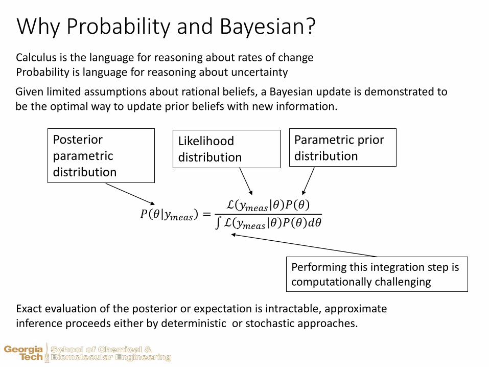
Why Probability and Bayesian?

Given limited assumptions about rational beliefs, a Bayesian update is demonstrated to be the optimal way to update prior beliefs with new information.

𝑃 𝜃 𝑦𝑚𝑒𝑎𝑠 =ℒ 𝑦𝑚𝑒𝑎𝑠 𝜃 𝑃 𝜃

ℒ 𝑦𝑚𝑒𝑎𝑠 𝜃 𝑃 𝜃 𝑑𝜃

Calculus is the language for reasoning about rates of changeProbability is language for reasoning about uncertainty

Posterior parametric distribution

Likelihood distribution

Parametric prior distribution

Performing this integration step is computationally challenging

Exact evaluation of the posterior or expectation is intractable, approximate inference proceeds either by deterministic or stochastic approaches.

Bayesian Machine Learning

𝑃 𝜃 𝐷,𝑚 =𝑃 𝐷 𝜃,𝑚 𝑃(𝜃|𝑚)

𝑃(𝐷|𝑚)

Machine Learning: Making inferences about missing or latent data from the observed data

A well defined model: Make predictions about unobserved data

m = model structureq = model parameters

𝑃 𝐷𝑡𝑒𝑠𝑡 𝐷,𝑚 = 𝑃 𝐷𝑡𝑒𝑠𝑡 𝜃, 𝐷,𝑚 𝑃 𝜃 𝐷,𝑚 𝑑𝜃

Make a prediction Using the posterior as the prior

𝑃 𝑚 𝐷 =𝑃 𝐷|m 𝑃(𝑚)

𝑃(𝐷)𝑃(𝐷|𝑚) = 𝑃 𝐷 𝜃,𝑚 𝑃 𝜃 𝑚 𝑑𝜃

Compare models

Example of Bayesian analysis in Process Systems Engineering: An adsorption process

• Data Fusion for isotherm data – multiple sources can be integrated seamlessly in estimating parameters

• Uncertainty Quantification for cyclic process performance –determine the reliability of model prediction based on uncertainties in data and model

• Design of experiments – optimally design experiments to reduce the uncertainty in model prediction and process performance

Bayesian data fusion

• Adsorption isotherm equilibrium data of Uio66 (MOF adsorbent) on CO2 collected from NIST from 9 different experimental groups • at 7 different temperatures at various ranges of CO2 partial

pressure.

• Langmuir isotherm model used to fit the data and estimate four unknown parameters

CO2 Adsorption equilibrium capacity : 𝑞𝑒𝑞 = 𝑞𝑚𝑏𝑃

1+𝑏𝑃

Maximum CO2 saturation capacity : 𝑞𝑚 = 𝑞𝑚0 exp 𝜂 1 −𝑇

𝑇0

Langmuir affinity constant: 𝑏 = 𝑏0 exp −Δ𝐻0

𝑅𝑇0

𝑇0

𝑇− 1

Bayesian Updating of Isotherm Parameters

• Dashed lines represent 95% credible intervals

Bayesian fit of all experimental data

• Each group’s data colored separately

• Different error measure for each group estimated and shown

– Some groups more accurate than others

New data addition to the fit

10

• New data from computational (molecular) simulations added.

– Increased uncertainty level because of error (std dev = 1.25) in

computational data (model uncertainties)

Molecular simulations data

Bayesian uncertainty quantification (UQ)

11

𝑃(𝜃|𝑦𝑚𝑒𝑎𝑠) 𝑃(𝑦𝑝|𝑦𝑚𝑒𝑎𝑠)

Uncertainty propagation (step 2)

Model

Noisy and uncertain

measurements

Estimate posterior predictive

distribution

Parameters 𝜃 Prediction variable 𝑦𝑝

Parametric inference (step 1)

Estimates model and parametric uncertainty

Impact of uncertainties on model prediction

Estimate posterior

parametric distribution

Application study : Cyclic adsorption process to capture CO2 from flue gas

Self SweepingAdsorption

N2 sweepingCooling

Rapid Thermal Swing Adsorption (RTSA) with a hollow fiber module

1. Kalyanaraman J et al.. Modeling and experimental validation of carbon dioxide sorption on hollow fibers loaded with silica-supported poly(ethylenimine). Chem.Eng.J. 2015;259:737-751.

120 o C

120 o C

Cooling N2 sweeping

Cyclic process model and the measured experimental data

• Totally 10 unknown model parameters to be estimated.

• Model composed for eight coupled PDEs - takes around 5 minutes to simulate the adsorption step alone and 40-50 minutes to reach cyclic steady state.

• CO2 breakthrough profile in adsorption step used to estimate unknown parameters (8 experimental data at varying conditions)

Likelihood distribution ℒ 𝒚𝒎𝒆𝒂𝒔 𝜽• Measure of how likely the model with parameters 𝜃, fits the data 𝑦𝑚𝑒𝑎𝑠

• Assumes a Gaussian distribution for errors (model mismatch)

𝑦𝑚𝑒𝑎𝑠,𝑖 = 𝑦𝑚𝑜𝑑𝑒𝑙,𝑖 𝜃 + 𝜖

𝜖 ~𝒩 0, 𝜎𝑒2 ; 𝑖 = 1. . 𝑁 (no of experiments)

ℒ 𝑦𝑚𝑒𝑎𝑠 𝜃 = Π𝑖𝑁 1

2𝜋𝜎𝑒𝑒−𝑦𝑚𝑒𝑎𝑠,𝑖−𝑦𝑚𝑜𝑑𝑒𝑙,𝑖

2

2𝜎𝑒2

• For every sample value 𝜃, full forward simulation is run for each experiment to calculate likelihood

• Computationally expensive With CPU time of single simulation ≈ 5 − 6 𝑚𝑖𝑛 , SMC requires at least

2 weeks (8 experiments x 12 MCMC runs per iteration x 30 time iterations x 6mins)

Sequential Monte Carlo to determine P(𝜃|𝑦𝑚𝑒𝑎𝑠)

16

• Uses samples across the distribution to track

• Makes incremental updates to target distribution with 𝛾𝑡 exponent in likelihood

• Faster convergence

• Parallelizable – one sample tracking per processor

• In our case custom-built in Python and used in parametric inference for our example breakthrough data.

Jeremiah, E. et al, Water Resour. Res, 47,2011

Results on Parameter Estimation of Posterior distribution

Adsorption isotherm parameters

Mass transfer resistance parameters

Propagating the uncertain parameters through the cyclic model

CO2 mole fraction at the exit over the cycle without prediction error

Recovered stream

CO2 recovery of product stream without prediction error

CO2 purity of product stream without prediction error

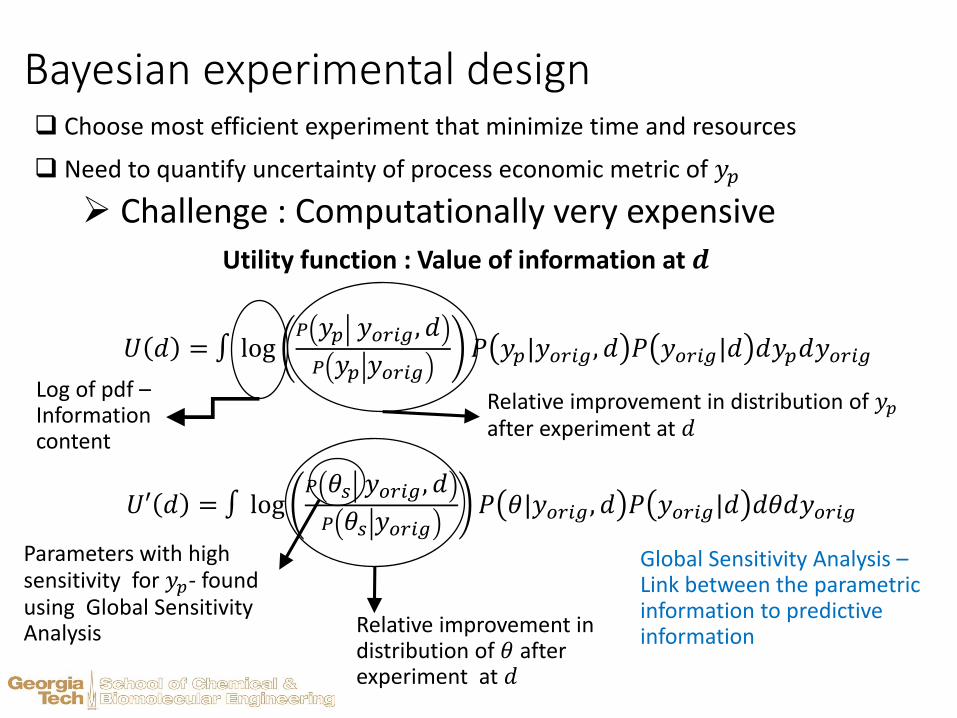
Bayesian experimental design Choose most efficient experiment that minimize time and resources

Need to quantify uncertainty of process economic metric of 𝑦𝑝

Challenge : Computationally very expensive

𝑈 𝑑 = log𝑃 𝑦𝑝 𝑦𝑜𝑟𝑖𝑔, 𝑑

𝑃 𝑦𝑝 𝑦𝑜𝑟𝑖𝑔𝑃 𝑦𝑝|𝑦𝑜𝑟𝑖𝑔 , 𝑑 𝑃 𝑦𝑜𝑟𝑖𝑔|𝑑 𝑑𝑦𝑝𝑑𝑦𝑜𝑟𝑖𝑔

Utility function : Value of information at 𝒅

Relative improvement in distribution of 𝑦𝑝after experiment at 𝑑

Log of pdf –Information content

𝑈′ 𝑑 = log𝑃 𝜃𝑠 𝑦𝑜𝑟𝑖𝑔 , 𝑑

𝑃 𝜃𝑠 𝑦𝑜𝑟𝑖𝑔𝑃 𝜃|𝑦𝑜𝑟𝑖𝑔 , 𝑑 𝑃 𝑦𝑜𝑟𝑖𝑔|𝑑 𝑑𝜃𝑑𝑦𝑜𝑟𝑖𝑔

Relative improvement in distribution of 𝜃 after experiment at 𝑑

Parameters with high sensitivity for 𝑦𝑝- found using Global Sensitivity Analysis

Global Sensitivity Analysis –Link between the parametric information to predictive information

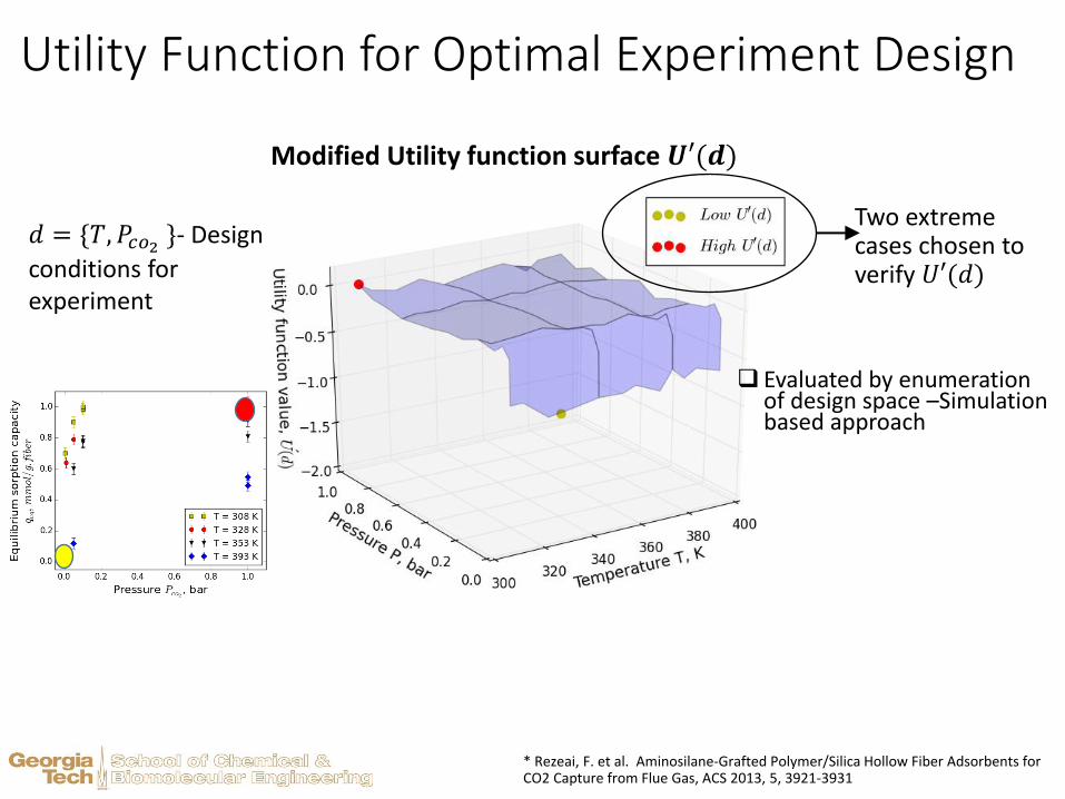
Utility Function for Optimal Experiment Design

𝑑 = {𝑇, 𝑃𝑐𝑜2 }- Design

conditions for experiment

Modified Utility function surface 𝑼′(𝒅)

* Rezeai, F. et al. Aminosilane-Grafted Polymer/Silica Hollow Fiber Adsorbents for CO2 Capture from Flue Gas, ACS 2013, 5, 3921-3931

Evaluated by enumeration of design space –Simulation based approach

Two extreme cases chosen to verify 𝑈′(𝑑)

23

Uncertainty Reduction by Optimal Experimental Design

Uncertainty comparison in Breakthrough capacity (design variable) prediction

Dashed lines indicate 95% credible intervals

Breakthrough capacity considering uncertainty increased from 0.605 to 0.63 mmol/g fiber( 5% increase) with one added data

Leads to ~ 5% reduction of net CO2 capture cost *

* Kulkarni and Sholl, Analysis of equilibrium based TSA processes for direct CO2 capture from air IECR (51), 2012

MILP Computing Performance 1988-2017Algorithm Performance 147,650xMachine Performance 17,120xCombined improvement = 2,527,768,000x = 2.5 billion times more effective

Overview of Mixed-integer Programming: Recent Advances, and Future Research Directions , Jeff Linderoth, University Wisconsin-Madison, FOCAPO 2017, Tuscon, Arizona, January 8th-12th.

http://www.lanl.gov/orgs/hpc/salishan/salishan2011/3moore.pdf

Are we reaching the limits of single-core performance improvements?

Shift towards increased number of cores.

Logical Reasoning and InferenceE.g. Boolean Satisfiability --SAT

https://www.cs.helsinki.fi/u/mjarvisa/papers/jarvisalo-leberre-roussel-simon.aimag.pdf

In 2011, the biggest application instance solved by at least one solver contained 10M variables, 32M clauses, and a total of 76M literals.

Efficient inference for large scale problems within 20 years.

Computational advances in MCMC and Bayesian analysis in last forty years

Algorithm Performance in terms of parallel algorithms 500x1

Complete parallelism of model evaluations 20x2

Machine Performance 17,120xCombined improvement = 1,712,000,000x = 1.7 billion times more effective

1. Workshop on recent advances in Bayesian computation, 20102. Amdahl’s law

• Parallel computation with SMC vs serial single threaded MCMC computation for Bayesian inference for a small isotherm model ( 8x speedup)

• For larger complex model speedup upto500x

Bayesian Process Systems Engineering 2040

Massively parallel probabilistic inference

Chemical engineering models driven by fundamentals

Ambient large datasets AND carefully designed small datasets

?