bayesian networks of dynamic systems
TRANSCRIPT

Habilitation a Diriger les Recherchesmention Informatique
Universite de Rennes 1
Bayesian Networksof Dynamic Systems
(Version du 28 Mars 2007)
Eric Fabre
Soutenue le 14 juin 2007, devant le jury compose de
President Michel Raynal, Prof. d’Informatique, Univ. Rennes 1
Rapporteurs Stephane Lafortune, Prof. of EECS, Univ. of MichiganAlan Willsky, Prof. of EE, MIT, Cambridge (US)Glynn Winskel, Prof. of CS, Univ. of Cambridge (UK)
Examinateurs Albert Benveniste, DR INRIA, IRISA, RennesChristophe Dousson, Resp. d’Eq. de Rech., France Telecom R&DAlessandro Giua, Prof. of EE, Univ. de Cagliari
IRISA/INRIACampus de Beaulieu35042 Rennes cedex

2

Contents
1 Introduction 71.1 Motivation . . . . . . . . . . . . . . . . . . . . . . . . . . . . . . . . 71.2 A distributed approach to monitoring problems . . . . . . . . . . . . 91.3 Overview of our contribution . . . . . . . . . . . . . . . . . . . . . . 111.4 Organization of the document . . . . . . . . . . . . . . . . . . . . . . 161.5 Historical perspective . . . . . . . . . . . . . . . . . . . . . . . . . . 17
2 Graphical models of interactions 212.1 Systems and their graphs . . . . . . . . . . . . . . . . . . . . . . . . 21
2.1.1 Systems . . . . . . . . . . . . . . . . . . . . . . . . . . . . . . 212.1.2 Examples . . . . . . . . . . . . . . . . . . . . . . . . . . . . . 232.1.3 Graphs of a compound system . . . . . . . . . . . . . . . . . 24
2.2 Distributed reduction algorithms . . . . . . . . . . . . . . . . . . . . 262.2.1 The reduction Problem . . . . . . . . . . . . . . . . . . . . . 262.2.2 Message passing algorithm . . . . . . . . . . . . . . . . . . . . 272.2.3 Turbo algorithms . . . . . . . . . . . . . . . . . . . . . . . . . 302.2.4 Involutive systems . . . . . . . . . . . . . . . . . . . . . . . . 34
2.3 Summary . . . . . . . . . . . . . . . . . . . . . . . . . . . . . . . . . 36
3 Networks of dynamic systems 393.1 Dynamic systems and their compositions . . . . . . . . . . . . . . . . 39
3.1.1 A category of multi-clock automata . . . . . . . . . . . . . . 403.1.2 Composition by product . . . . . . . . . . . . . . . . . . . . . 413.1.3 Composition by pullback . . . . . . . . . . . . . . . . . . . . 43
3.2 Graphs associated to a multi-clock system . . . . . . . . . . . . . . . 473.2.1 Direct graph . . . . . . . . . . . . . . . . . . . . . . . . . . . 473.2.2 Dual graph . . . . . . . . . . . . . . . . . . . . . . . . . . . . 48
3.3 Diagnosis problem . . . . . . . . . . . . . . . . . . . . . . . . . . . . 513.3.1 Semantics . . . . . . . . . . . . . . . . . . . . . . . . . . . . . 523.3.2 Objectives . . . . . . . . . . . . . . . . . . . . . . . . . . . . . 523.3.3 The diagnoser approach . . . . . . . . . . . . . . . . . . . . . 54
3.4 Distributed diagnosis : the language approach . . . . . . . . . . . . . 553.4.1 Diagnosis in terms of languages . . . . . . . . . . . . . . . . . 553.4.2 Diagnosis in terms of trajectories . . . . . . . . . . . . . . . . 563.4.3 Extensions and drawbacks . . . . . . . . . . . . . . . . . . . . 58
3

3.5 Trajectory sets in the sequential semantics . . . . . . . . . . . . . . . 593.5.1 Trellis automaton . . . . . . . . . . . . . . . . . . . . . . . . . 593.5.2 Time-unfolding of an automaton . . . . . . . . . . . . . . . . 603.5.3 Variations around the height function . . . . . . . . . . . . . 633.5.4 Categorical properties . . . . . . . . . . . . . . . . . . . . . . 64
3.6 Distributed diagnosis : the trellis approach . . . . . . . . . . . . . . . 663.6.1 Centralized diagnosis, single sensor . . . . . . . . . . . . . . . 663.6.2 Centralized diagnosis, several sensors . . . . . . . . . . . . . . 673.6.3 Distributed diagnosis . . . . . . . . . . . . . . . . . . . . . . . 67
3.7 Towards true concurrency semantics . . . . . . . . . . . . . . . . . . 713.8 Summary . . . . . . . . . . . . . . . . . . . . . . . . . . . . . . . . . 75
4 True concurrency semantics 774.1 Networks of automata as asynchronous systems . . . . . . . . . . . . 774.2 Multi-clock nets and their composition . . . . . . . . . . . . . . . . . 79
4.2.1 A category of multi-clock nets . . . . . . . . . . . . . . . . . . 794.2.2 Composition by product and pullback . . . . . . . . . . . . . 824.2.3 Graphs associated to a multi-clock system . . . . . . . . . . . 84
4.3 Trajectory sets in the true concurrency semantics . . . . . . . . . . . 844.3.1 Unfolding of a net . . . . . . . . . . . . . . . . . . . . . . . . 854.3.2 Factorization property . . . . . . . . . . . . . . . . . . . . . . 88
4.4 Distributed diagnosis : the unfolding approach . . . . . . . . . . . . . 894.4.1 Projection . . . . . . . . . . . . . . . . . . . . . . . . . . . . . 904.4.2 Centralized diagnosis . . . . . . . . . . . . . . . . . . . . . . . 924.4.3 Distributed diagnosis . . . . . . . . . . . . . . . . . . . . . . . 934.4.4 Example . . . . . . . . . . . . . . . . . . . . . . . . . . . . . . 964.4.5 Involutivity . . . . . . . . . . . . . . . . . . . . . . . . . . . . 99
4.5 Augmented branching processes . . . . . . . . . . . . . . . . . . . . . 1004.5.1 Definition . . . . . . . . . . . . . . . . . . . . . . . . . . . . . 1004.5.2 Key property . . . . . . . . . . . . . . . . . . . . . . . . . . . 1024.5.3 Operations on ABP : product, pullback, projection . . . . . . 1034.5.4 Separation theorem . . . . . . . . . . . . . . . . . . . . . . . 1064.5.5 Weak involutivity . . . . . . . . . . . . . . . . . . . . . . . . . 106
4.6 Summary . . . . . . . . . . . . . . . . . . . . . . . . . . . . . . . . . 108
5 Trellis unfolding for concurrent systems 1115.1 Trellis nets . . . . . . . . . . . . . . . . . . . . . . . . . . . . . . . . 111
5.1.1 Definition . . . . . . . . . . . . . . . . . . . . . . . . . . . . . 1125.1.2 Trellis process and time unfolding of a net . . . . . . . . . . . 1165.1.3 Factorization properties . . . . . . . . . . . . . . . . . . . . . 118
5.2 Relations to unfoldings . . . . . . . . . . . . . . . . . . . . . . . . . . 1195.2.1 Variations around the height function . . . . . . . . . . . . . 1195.2.2 Nested co-reflections . . . . . . . . . . . . . . . . . . . . . . . 120
5.3 Distributed diagnosis : an example . . . . . . . . . . . . . . . . . . . 1225.4 Summary . . . . . . . . . . . . . . . . . . . . . . . . . . . . . . . . . 123
4

6 Applications, contracts, technology transfer 1276.1 MAGDA . . . . . . . . . . . . . . . . . . . . . . . . . . . . . . . . . . 1276.2 MAGDA 2 . . . . . . . . . . . . . . . . . . . . . . . . . . . . . . . . . 1306.3 VDT . . . . . . . . . . . . . . . . . . . . . . . . . . . . . . . . . . . . 132
7 Conclusion 1357.1 Summary of results . . . . . . . . . . . . . . . . . . . . . . . . . . . . 1357.2 Directions for future work . . . . . . . . . . . . . . . . . . . . . . . . 137
7.2.1 Technical extensions . . . . . . . . . . . . . . . . . . . . . . . 1377.2.2 Research directions . . . . . . . . . . . . . . . . . . . . . . . . 138
8 Acknowledgement 141
5

6

Chapter 1
Introduction
“(...) diviser chacune des difficultes que j’examinerais, en autant deparcelles qu’il se pourrait, et qu’il serait requis pour les mieux resoudre.
(...) conduire par ordre mes pensees, en commencant par les objets lesplus simples et les plus aises a connaıtre, pour monter peu a peu, commepar degres, jusques a la connaissance des plus composes ; et supposantmeme de l’ordre entre ceux qui ne se precedent point naturellement lesuns les autres.”
Rene Descartes, in Discours de la methode 1 (1637)
1.1 Motivation
The decomposition principle splitting a complex task into simpler subtasks, hasfounded decades of technological achievements. Most systems we commonly use ev-ery day involve complex chains of reactions between components of different scales,that combine to form the service we expect from them. Assembling components toform a more powerful system is so efficient and widespread that it almost forms acommonplace to mention it. However, considering with more attention the complex-ity levels of current systems, and the way they are designed today, suggests that thisparadigm has reached some limitations.
1. Size. The most obvious limitation : The explosive number of elements involvedin some applications now reaches complexity levels that go far beyond what asingle person can master.
2. Historical constraints. Very often, redesign from scratch has become in-tractable or simply too expensive, or is impossible for matters of downward
1Among the four principles of the method, these are the 2nd and 3rd ones. In substance, 1/ takenothing for granted, 2/ divide a complex problem into simpler sub-problems, 3/ understand eachelementary sub-problem, and recombine, 4/ don’t forget anything ! Summarized as “divide andconquer” by fast readers.
7

compatibility. So one is bound to continuously upgrade parts of an exist-ing system or software, which leads to a discrepancy between recent and oldtechnologies, recent and old design paradigms.
3. Heterogeneity. In the same way, there is also a trend to rapidly assembleoff-the-shelf components, of different generations and manufacturers, in orderto follow the market demand or new offers proposed by competitors. Thisproduces systems that sometimes have unexpected behaviors, whence the ne-cessity of heavy test procedures. As a matter of fact, most softwares or servicestoday are delivered in a continuous flow of versions, following a continuous flowof bug reports.
4. Open systems. In many cases, compound systems are no longer closed sys-tems, like a chip, a computer or a plane, for which the manufacturer couldtheoretically master all components. They are rather open systems, only par-tially known to people in charge of their monitoring. In particular in the fieldof telecommunication networks, or of distributed softwares.
5. Unstructured systems. After decades of hierarchical decomposition intocomponents, new design paradigms appear under the form of peer architec-tures, where components are both clients and servers of one another. Muchless intuitive objects in terms of management.
6. Dynamic architectures. Moreover, the structure itself of some current soft-ware systems is no longer stable and designed once for all, but may be built“on demand.” This was partly the case in telecommunication networks, butit becomes a central feature in peer-to-peer networks or in web services, twofast growing application paradigms.
One may be happy with this situation, as far as the main function of a complexsystem is globally satisfied, and continuously improved by a “test and modify” pro-cess. But of course, this can’t be sufficient for critical applications. New tools andconcepts are continuously needed to assess beforehand whether a system fulfills itsobjectives or not, whether it is error-free or not. And once a large system hasbeen deployed, similar difficulties remain at run time to monitor it and analyze itsbehavior, which is the topic of this document.
As a typical domain where these issues are becoming of critical importance, letus mention telecommunication networks and services management. It is by nowconsidered that network elements (NE) are so complex and offer so many featuresand adjustable parameters, meanwhile networks increase in size and heterogeneityof equipment and functions, that the traditional monitoring of a network by directlyaccessing and tuning NEs has become impossible. It is commonly considered thata human operator needs one year to master a new NE technology and be able toparameterize the network he supervises. Research groups like the NMRG (Net-work Management Research Group) at IRTF (Internet Research Task Force), or theEuropean research network EMANICS (MANagement of Internet technologies andComplex Services), are now orienting research to new management concepts. Under
8

the generic name of autonomic communications, objectives like self-configuration,self-healing, self-adaptation, self-xxx reveal a trend to abstract the inherent com-plexity of systems and search for high-level programming mechanisms for telecom-munication networks. Ideally, one should be able to program a network by assigningit service-level objectives. What technologies will bridge the gap between thesehigh-level objectives and low-level management is still unclear and remains a veryactive research field. One trend is to push down these high-level requirements, un-der the form of policy-based management (essentially for performance management).Another strong tendency favors probabilistic methods, both to model network be-haviors (performance and configuration management), or to understand its behavior(learning methods or statistical techniques for fault management and event correla-tion).
The research work we summarize in this document addresses complexity issuesin the reverse direction. We start from traditional model-based approaches to somemonitoring problems, that were successful so far for small size systems, and proposea methodology to extend them to possibly large networks of components. Theidea is quite simple : the complexity of networked systems precisely comes fromthe existence of many interconnected functions and elements. Why not turningthis to our advantage and imagining a monitoring architecture that would itself bedistributed ? Ideally, this would both solve scalability issues, and allow a naturalupgrade of monitoring architectures as the structure of the supervised system isupdated. As a matter of fact, we’ll see that our approach naturally leads to thefashionable idea of peer to peer monitoring architectures, but with a sound algebraicbasis.
Most of this research was motivated by a target application : failure diagnosis intelecommunication networks. The results we obtained have been successfully imple-mented and tested on different network technologies, in cooperation with industrialpartners2. But beyond these direct applications, the theory seems rich and promis-ing enough to address some of the difficulties mentioned above. For example systemswith a varying structure, like Web Services. Very likely also, off-line problems likemodel checking for large components can be addressed with this approach. In sum-mary, between small systems that can be studied as a whole, and large ones thatcan only be built and tested, or modeled with probabilistic methods, there seems tobe some accessible land to explore.
1.2 A distributed approach to monitoring problems
We focus on discrete event dynamic systems (DEDS), and in particular on dis-tributed systems obtained by assembling a large number of components, that wecould also call networks of dynamic systems. Such systems very rapidly becomeintractable as their size augments. This is due to combinatorial explosions that takeplace both in their state space, and in their trajectory space. Because of these com-
2Experiments have been carried out for SDH optical network, MPLS networks, submarine lineterminal equipment, and GSM radio access network. Alcatel R&I is currently evaluating the intro-duction of this technology into ALMAP, its corporate network management platform.
9

binatorial explosions, global (or centralized) approaches developed for monitoringproblems are no longer applicable. By “monitoring problem,” we encompass prob-lems like supervisory control, optimal control, optimal state/trajectory estimation,or diagnosis problems. Several authors have proposed to address the challenge ofdistributed systems by means of distributed (or modular) methods. The centralidea is to solve the target monitoring problem by parts, at the scale of a single com-ponent, in such a way that combining local/partial solutions gives the global one.Specifically, there exist two strategies to do so3 :
• In the decentralized monitoring architecture, a local supervisor is attached toeach component (or group of), and has only a local knowledge : it only knowsthe model of that component, plus interface information with the rest of thesystem, and only has access to observations/measurements coming from thatcomponent. Local supervisors perform some computations and forward theirresults to a coordinator in charge of assembling them. This coordinator issupposed to ignore everything about the supervised system, and has minimalcomputation capabilities, which means that most of the work is performed bylocal supervisors.
• In the distributed architecture, one is not so much interested in computing aglobal solution to the monitoring problem, like a global diagnosis, estimates ofglobal states, etc. On the contrary, only local views of these global solutionsare of interest, that is their projections on each component. Therefore thecoordinator becomes useless. The monitoring architecture simplifies into acollection of local supervisors, one per component, having local knowledgeand coordinating their work with supervisors of neighboring components toprovide a set of coherent local views.
The methodology we propose belongs to the second class, which can be consideredas a generalization of the first one, where the necessity of a coordinator is relaxed.The advantage is obvious in terms of scalability : each time a new component isincorporated or replaced into the system, one only has to connect/replace its cor-responding local supervisor to upgrade the monitoring architecture (Fig. 1.1). Thefact that the connectivity of the supervising architecture must be isomorphic to theinteraction structure between components in the system is not casual and will becommented in the next chapters. Notice also that although the knowledge aboutthe “global solutions” to the monitoring problem is distributed in this approach, theinformation is nevertheless present and available for standard post-processings (likeresult report, action decision, etc.).
At this point, we made no distinction between modular and distributed process-ings. The modularity refers to a problem that can be solved by parts, where eachcomputation “module” is based on a limited knowledge. Typically, computations
3In this classification, we omit contributions that do not take into account the modularity ofthe supervised system. For example approaches where several sensors collect different observationson a unique component. Although these approaches are interesting in terms of cooperation be-tween sensors, the modular processing is generally as complex as a global processing based on allobservations. Our goal here is to reduce complexity, in order to capture large systems.
10

new localsupervisor
Superv
ised s
ystem
plan
eDistrib
uted m
onito
ring p
lane
interaction component
local supervisor collaboration
new component
Figure 1.1: A network of dynamic systems, and its distributed monitoring architec-ture.
performed by a local supervisor, knowing only one component and observations thatit produced. The expression “distributed processing” goes further by assuming thatthe partial computations are performed at different locations, and thus require com-munications between modules. This introduces scheduling issues in the problem :one first has to determine what should be computed locally, what to communi-cate to neighbors, but also when communication should take place, and what to dowith delayed (or lost) messages. These protocol concerns are very sensitive in someapproaches [90]. In the framework presented here, we will consider asynchronousdistributed systems, and the distributed monitoring algorithms will also be com-pletely asynchronous. Therefore modularity will be equivalent to distribution, andwe shall not distinguish them.
1.3 Overview of our contribution
As suggested by the title, this document describes an attempt at assembling twodisconnected sets of results, developed in different communities and with apparentlyunrelated objectives.
Bayesian networks. The term Bayesian Network4 refers to graphical modelsdisplaying the correlation structure of a collection of random variables. Let V ={Vk, 1 ≤ k ≤ K} be a finite set of variables, and let V = V1 ∪ . . .∪ VN be a coveringof V, with Vn ⊆ V, 1 ≤ n ≤ N . We denote by v a function associating to eachvariable in V a value of its domain, and by vi we denote the restriction of v to Vn.We also denote vk a value of variable Vk. A joint distribution PV on variables V canbe specified in terms of so-called potential functions φn defined on the vn and takingvalues in R. Specifically
P(v) =1Z
exp {−N∑
n=1
φn(vn)} (1.1)
4Sometimes also called Markov random field, graphical model, or belief network, according tothe community using it.
11

where Z is a normalizing factor. Each subset Vn is called a clique. Intuitively φn
defines (soft) constraints on the elements of clique Vn, and by suitably combining allthese local constraints, one specifies the global correlation structure in V. To preparethe analogy with dynamic systems, we call the pair Sn = (Vn,φn) a component.
V4
V2
V3
V1
V5
V6
V7 V8
V7V4V1
V2 V5
V3 V6
V8V1
V2
V4
V5
V3
V7 V8
V6
− d −
− b −
− c −
− a −
S1
S3
S4
S2
S1 S4S2
S3
S1
S4
S2
S3
Figure 1.2: Four graphical representations of dependencies between variables Vk
and/or components Sn.
The interactions in V admit several graphical representations.
• The most direct : as a hypergraph H = (V, {Vn}1≤n≤N ). Every variable in Vis a node, and each subset Vn defines a hyper-edge (Fig. 1.2-a).
• As a graph G = (V, E), still with variables as nodes. Two variables are relatedby an edge of E iff they appear in the same Vn, for some n. Or equivalently,G restricted to Vn is a complete graph (Fig. 1.2-b).
• As a bipartite graph G = (V, S,E). One still has variable V as first set ofnodes, and the second one S = {1, . . . ,N} corresponds to the N “systems”defined by the Vn. A variable V ∈ V is related by an edge to system n iffV ∈ Vn (Fig. 1.2-c).
• As a dual graph G = (S,E) where nodes in S = {1, . . . ,N} still represent theVn. There is an edge in E between n and m iff Vn ∩ Vm '= ∅ (Fig. 1.2-d).
These graphical representations have two main advantages.
1. First of all, they can be directly interpreted in terms of conditional indepen-dence statements. Consider Fig. 1.2-b for example. Variables {V4, V7} sepa-rate {V1, V2, V3, V5, V6} from {V8} in the sense that removing V4 and V7 from
12

the graph disconnects these two sets. This property immediately entails that(V1, V2, V3, V5, V6) and V8 are conditionally independent given (V4, V7) for P :
P(v) = P(v1, v2, v3, v5, v6|v4, v7) P(v8|v4, v7) P(v4, v7) (1.2)
as it can be checked directly from (1.1). The graph is thus a summary of a setof conditional independence relations. Whence the name “Bayesian network : ”(1.2) is a Bayes formula.
2. Secondly, precisely because of these conditional independence relations, es-timation problems can be resolved by parts. These problems typically takethe following form : one observes the value of some variables in V and wishesto determine the most likely value of all the others. In the simplest cases,i.e. when the interaction graph of fig. 1.2-d is a tree, the resolution takesthe form of message passing algorithms (MPA), where some computations areperformed at the scale of a single clique Vn, and where neighboring cliquesexchange messages. The most famous examples of such algorithms appearfor Markov chains, i.e. Bayesian networks where the cliques are organizedin a single string : the Viterbi algorithm, the soft output Viterbi algorithm(SOVA), the Kalman filter, the Rough-Tung-Striebel algorithm, the Bahl-Cocke-Jelinek-Raviv (BCJR) algorithm, the forward-backward algorithm, the[min,max]-[sum,product] algorithm, the sum-product algorithm, dynamic pro-gramming, the belief propagation are all examples of MPA5. For more complexgraphs, MPA can still be applied. They are theoretically suboptimal, but yieldexcellent results in practice, as it was revealed by the iterative algorithms fordecoding turbo-codes.
The reader will have noticed that message passing algorithms are a form of dis-tributed processings. We are precisely going to elaborate on this remark.
Networks of dynamic systems. The simplest model of a discrete event dynamicsystem (DEDS) takes the form of an automaton A = (Q,T, v0). A is composedof a single state variable V taking values in the finite set Q of possible states,and initialized at v0 ∈ Q. T ⊆ Q × Q is a finite set of transitions : a transitiont = (v, v′) ∈ T can fire when V takes value v. After the firing, A is in stateV = v′. A run of A is thus a sequence σ = v0[t1〉v1[t2〉v2 . . . vl−1[tl〉vl . . . such thattl = (vl−1, vl) ∈ T .
With a very simple idea, this class of DEDS can be extended to encompassmuch more complex systems : instead of a single variable V , we can define automataoperating on several state variables. Specifically, we define a tile system S as a tripleS = (V,T ,v0), where V = {Vk, 1 ≤ k ≤ K} is a set of variables with finite domains,T is a finite set of tiles, and v0 is the initial “state” of the system. Apparently, weonly introduced a vector-valued state variable. The originality comes from the factthat transitions of T , that we call tiles , do not operate on all variables at a time.A tile t = (Vt,v−
t ,v+t ) ∈ T modifies only variables in Vt ⊆ V. Specifically, t can
5Often the same algorithm appears with different names, according to the community that(re)discovered it !
13

fire when the state v of the system restricted to Vt takes value v−t . After the firing,
these variables are changed to value v+t , and variables in V \ Vt remain unchanged
(fig. 1.3). This formalism is very convenient to define large systems, with numerousstate variables, by local dynamics.
o1
o3
o2
o4
V1 V2 V3 V4
v01 v0
2 v03 v0
4
v’1 v’2 v04v0
3
v03v’2v’1
v’1 v’3v"2
v’4
v’4
v"3 v"4v’1 v"2
S1 S2
Figure 1.3: A run of a tile system made of two components S1 and S2, that sharetwo variables, V2 and V3. The first tile firing in this run (top left) changes only thevalue of V1 and V2, and produces the label o1.
The main advantage of this framework is that tile systems can be composedvery naturally. There exists several ways to define the composition, that we shallrecall in this document. The simplest one, at this point, is the following : let theSn = (Vn,Tn,v0
n) be tile systems, 1 ≤ n ≤ N , their composition S = (V,T ,v0) =S1‖S2‖ . . . ‖SN is obtained by taking the union of variables V = V1 ∪ . . . ∪ VN
and of tiles T = T1 ∪ . . . ∪ TN , and by assembling the initial states v0i (provided
they coincide on shared variables). The interactions come from the fact that twocomponents Sn,Sm can both read and change the values of the state variables in theintersection Vn ∩ Vm. The latter thus behave as communication ports.
As for Bayesian networks, one can associate graphical representations to a com-pound tile system S, and they turn out to be exactly those of Fig. 1.2 ! Insteadof a potential function φn defining constraints on a subset Vn of variables, on hasa component Sn defining local dynamics on the Vn. But we need one more step tomake this analogy operational.
The join. In its simplest form, a monitoring problem for S could be expressed asfollows. Assume some of the tiles in the Sn can emit a possibly random signal whenthey fire (the production of an alarm for example) that we call a label. S performsa hidden run κ, and the labels emitted by tiles in this run are collected under theform of observations Ob (Fig. 1.3). Since κ is hidden, the goal is to recover all runs
14

of S that could have produced Ob. Further, if each component Sn is a stochasticsystem, one would like to recover the most likely run, as an estimate of κ.
This problem looks very much like a standard Hidden Markov Model (HMM)problem. But here, we complexify it a little.
• First we assume that observations Ob are not collected into a single sequenceof labels. Rather, labels are collected on each component Sn by a local sensor,that produces the local observation set Ob
n. Our observation is thus the tupleOb = (Ob
1,Ob2, . . . ,Ob
N ), and the interleaving of events in the Obi is assumed to
be lost.
• Secondly, as mentioned in the previous section, we aim at possibly large sys-tems. Therefore the usual procedures for HMMs, that operate on the statespace of S, are just unaffordable : the state space size explodes with the num-ber of components. We rather look for a modular methodology to solve themonitoring problem, where computations would be performed at the scale ofcomponents Sn.
• Finally, we would like to perform this monitoring on-line, i.e. we wish toupdate our estimates of the hidden run κ on the fly, as new observations arecollected on the different sensors.
This is close enough to the MPA we sketched for Bayesian networks. To establishthe connection, one must realize that the objects we are interested in are not so muchthe components Sn themselves, but rather their sets of runs. So we must introducetime in our formalism. As illustrated in Fig. (1.3), a run κ of S can be consideredas a tuple of trajectories (i.e. sequences of events), one per variable Vk. So let usdenote by Vk a variable whose values are trajectories of Vk, for Vk ∈ V. We are goingto use the fact that variables (Vk)1≤k≤K form a “Markov field,” in a very specificsense. Consider an operator U that would take a tile system S and compute in someform or another the set U(S) of all its runs κ. We will show in this document thatU can be designed so as to be a product preserving functor on tile systems. In otherwords, one has
U(S1‖ . . . ‖SN ) = U(S1) ∧ . . . ∧ U(SN ) (1.3)
where ∧ is an appropriate composition operator on trajectory sets.This factorization property is the counterpart of (1.1) for networks of dynamic
systems, and is at the core of the methodology we present in this document. EachU(Sn) can be considered as a “potential function” or as the definition of local con-straints on variables Vn = {V , V ∈ Vn}. Because of (1.3), the interaction structureof the U(Sn) is identical to that of the components Sn themselves. Finally, obser-vations Ob
n as well can be interpreted as some knowledge on the local trajectoriesin U(Sn), i.e. on the values of variables in Vn. So we are almost back to a staticproblem that can be solved by MPA.
This forms the essential message of this document : many results obtainedfor Bayesian networks can be recycled into distributed and asynchronousestimation algorithms for distributed dynamic systems.
15

1.4 Organization of the document
The next chapter describes an axiomatic framework designed to capture both Bayesiannetworks and networks of dynamic systems. The objective is to describe messagepassing algorithms (MPA) in a formalism that encapsulates both situations. We de-fine abstract systems operating on variables, that we compose by shared variables.Only two operators are useful on these systems : a composition and a projection (orreduction). We relate them by a small set of axioms, from which many algebraicproperties can be derived. The interaction structure of a compound system can bedescribed by a graph, on which the standard separation criterion is equivalent toa form of conditional independence. This is sufficient to develop MPA, study theirconvergence and explore the properties of their stationary points.
Chapter 3 is a first application of this framework to dynamic systems, in the sim-plest possible setting. We define a network of dynamic systems as the compositionof automata by the usual parallel product. This composition is slightly modifiedto keep track of components when they are assembled. Such systems are providedwith the usual sequential semantics : their runs are simply sequences of events. Thedistributed diagnosis problem is defined in this setting, and solved in different ways.First of all we reason on languages, which highlights the architecture of the compu-tations that we apply all along this document. But languages are very inefficient toencode large sets of runs of a system, so they are inappropriate to on-line monitoringalgorithms. The notion of trellis process is then introduced to describe sets of runsin a compact manner. We show that these objects enjoy a nice factorization prop-erty and satisfy the axiomatic framework of chapter 2, which allows us to computewith them. The key point here,i.e. the factorization property of trellis processes, isderived by category theory arguments. We conclude this chapter by showing somedrawbacks of the sequential semantics, and advocate true concurrency semantics todeal with distributed systems.
Chapter 4 proposes a first setting to handle sets of runs in the true concurrencysemantics. We first change the notion of composition in order to preserve the statevariables of components, rather that merging them in a big product state variable.As in the case of networks of automata, composition can be done either by productor by shared components : both situations are equivalent. The notion of system thisleads to turns out to be almost equivalent to safe Petri nets. In the true concurrencysemantics, runs are partial orders of events (or Mazurkiewicz traces), and sets of runscan be encoded under the form of branching processes. The latter enjoy once again anice factorization property (still derived by category theory arguments), and admita natural notion of projection. However, the axioms of chapter 2 are satisfied only invery specific cases. To perform computations in the general case, one must introducethe notion of augmented branching process.
Chapter 5 tries to go further and explores the existence of trellis processes forthe true concurrency semantics, as an even more compact way of encoding sets ofruns. Still in view of efficient distributed and on-line monitoring algorithms. Trellisprocesses can indeed be defined, and enjoy very elegant properties. In particular, thefactorization property is preserved, and a natural notion of projection exists, which
16

allows us once again to apply the formalism of chapter 2 in some specific cases. Butthe notion of augmented trellis process, that would encompass the general case, isstill missing.
Chapter 6 gives some snapshots at different contracts that guided this research.It describes the applications that were considered and some features of the proposedsolutions. It underlines in particular how the implementations that were experi-mented were either in advance, or late, or sometimes erroneous with respect to thedevelopment of the corresponding theory.
As a conclusion, chapter 7 summarizes the state of this theory and identifies somemissing tiles in the puzzle. It also lists a number of immediate or more futuristicextensions of this work.
1.5 Historical perspective
The assembling of Bayesian networks, distributed dynamic systems and categorytheory presented in this document doesn’t yet form a completely smooth theory.But it already went through several polishing phases. We briefly mention some ofthem to underline the benefits of crossing different scientific cultures, but also toshow how simple ideas sometimes take complex ways to materialize, ways in whichchance plays an important part.
The origins. The problem that triggered this research was jointly raised in 1996by Claude Jard (background in distributed programming) and Albert Benveniste(several backgrounds, in particular signal processing and random processes). Intelecommunication networks, failures generally propagate in the net which causesbursts of alarms at different locations. These alarms are only partially ordered intime, due to the distributed nature of the network. So the original problem was toidentify failures from patterns of partially ordered alarms. The idea of interactingcomponents and of stochastic systems were also present at the very beginning, whichoriented us to Bayesian networks.
V4
V2 V3V1V4
V2 V3V1V4
V3V1 V2
timet+1
t
t!1
Figure 1.4: Augmenting interactions in space with interactions in time.
Very soon however, we were faced with the difficulty of introducing time, ordynamics, in Bayesian networks. When there is a single state variable, for example
17

in Markov chains, this is done by duplicating the variable to represent its value ateach clock tick. Time is unfolded, in some sense. And the Markov chain dynamicsis introduced by potential functions coupling variables at time t and t + 1. Appliedto a Bayesian network, this principle would amount to add one more dimension toFig. 1.2, perpendicular to the page, that would represent the time axis (Fig. 1.4).But in a distributed system, time is not homogeneous for all variables : as illustratedin Fig. 1.3, some variables may evolve while others remain constant. And the placeswhere transitions occur depend the run ! To capture this unusual feature, one wouldneed a Bayesian network (or a Markov random field) whose structure would dependon the value of some of its variables. Unfortunately, such a theory doesn’t exist yet,and seems difficult to conceive.
Petri nets. It was thus chosen to abandon the idea of a global stochastic modelcapturing both interactions in space and in time. The first framework was based onpartially stochastic safe Petri nets. Petri nets are a natural model for concurrentsystems : they describe well the idea of local transitions, and the true concurrencysemantics allows us to describe their runs as partial orders of events, also calledconfigurations. The term “partially stochastic” relates to the fact that transitionshave a “weight,” related to their likelihood, which allows us to compare runs. How-ever no proper probabilistic space of runs was derived. This setting was sufficient toperform a Viterbi-like algorithm, and recover the “most likely” trajectory explaininga sequence (or a tuple of sequences) of alarms.
Estimation algorithms were soon extended into distributed procedures, for netswith several components connected by shared places. The key observation wasthat configurations of the global net could be split into local configurations of itscomponents. The resulting algorithm took the form of several cooperating Viterbialgorithms : one per component, in charge of recovering configurations of this com-ponent, and proposing to neighbors its possible explanations for shared places. Afterall observations were processed, a belief propagation phase was initiated to find thebest combination of local explanations.
Unfoldings. Handling sets of configurations can be quite heavy since these objectsrapidly become large. To minimize the memory space, configurations were encodedwith a back-pointer notation, as in [35, 31]. In other words, the underlying datastructure we used was the unfolding of the system, and a configuration was nothingmore than a tuple of entry points in this data structure. This revealed that thediagnosis could probably be performed directly in terms of unfoldings, which wasdone in [9]. Moreover, the distributed version of the algorithm suggested that theunfolding of a compound system factorized into local unfoldings. This was estab-lished directly in [37], and distributed estimation algorithms were re-expressed inthis setting : messages were now pieces of unfoldings.
Several results were then obtained in parallel. First of all, the derivation of an ax-iomatic framework to express general message passing algorithms (MPA) and studytheir algebraic properties [38]. In particular to express conditional independence,and study convergence of MPA. Secondly, the introduction of augmented branch-ing processes (ABP), as the correct framework to express distributed algorithms
18

(ordinary branching processes are not sufficient) [40]. Finally, the expression of dis-tributed algorithms in terms of event structures, instead of branching processes [41].
Factorization properties and category theory. By a strike of fate, while Iwas exploring different families of event structures to check if ABP already existed, Icame aware of Winskel’s work on models for concurrency. I was struck in particularby a result in [110], stating in a couple of lines the factorization property (1.3)on unfoldings6. The key argument for this derivation was some obscure result incategory theory... which I thus decided to investigate, motivated by the tediousproofs in [37]. And by Winskel’s killing sentence in [110] :
Proving these facts directly from the unfolding construction is quite un-wieldy - and completely uninstructive - so it is fortunate there is thisabstract characterization of the occurrence net unfolding of a [safe] net.In a sense, it was there all the time, because (...), so it was determined(...) by the categorical set-up.
The category theory approach brought many advantages, by focusing develop-ments on the essential features, while saving us from tedious and useless proofs.For example, interactions between components can be expressed under the form ofsynchronous products, or by shared variables (pullbacks [43]), without changing thetheory. Several other event structures were also quickly derived, like trellis processesfor the true concurrency semantics [45], or trellises for the usual interleaving seman-tics [44, 42], and their factorization properties came almost for free, thus makingthem available to distributed algorithms.
Markov nets. These elements of history wouldn’t be complete without mention-ing the collaboration with Stefan Haar, met at a workshop on Petri nets (GDRARP7, June 2000) where I was invited to give a talk about partially stochastic Petrinets. Just like us, Stefan was trying at that time to randomize concurrent systems.The difficulty was to obtain some equivalence between concurrency and stochasticindependence. In other words, components that do not interact should also be in-dependent in the stochastic sense, which is not achieved in any form of stochasticPetri nets. Combining our approaches, Albert, Stefan and I managed to randomizeunfoldings of a reasonable class of safe nets, and to define a Markov property on un-foldings, based on a notion of stopping time. This resulted in Markov nets [39], thatwas later refined by Samy Abbes who introduced the simpler notion of branchingcell (see Samy’s thesis [1] and [2]). Notice however that the availability of a genuinestochastic framework is important for identification issues, or performance analysis,but it has little influence on estimation algorithms, where one is only interestedin comparing the relative likelihoods of two trajectories ; so a definition “up to aconstant” is sufficient.
6This paper was handed to me by Samy Abbes, for a completely different purpose.7A CNRS funded research group, dedicated to architectures, networks and systems, and paral-
lelism.
19

20

Chapter 2
Graphical models of interactions
The formalism presented in this chapter aims at a double objective. First of all, wewant to introduce the minimum amount of concepts allowing us to define graphicalmodels of interactions and message passing algorithms. The idea is that the simplerthe formalism, the broader its scope. Secondly, with these simple tools, we want togo as far as possible in terms of distributed algorithms, convergence properties, etc.
We thus start with a simple definition of systems, “operating” on variables, andtwo operations. The first one allows us to compose systems, the second one allowsus to reduce systems to part of their variables. With a simple set of axioms on thesetwo operators, in particular a form of conditional independence property, one canderive interaction graphs of systems and message passing algorithms. In some cases,convergence properties can be established. This formalism is the basis on whichdistributed algorithms will be built, when we move to networks of dynamic systems.
2.1 Systems and their graphs
Notations. Specifying the notations of the introduction, we consider a finite setVmax of variables. A variable V ∈ Vmax takes values v in domain DV . Variablesets are denoted with script letters V ⊆ Vmax, and bold-face letters like v representfunctions over V, associating a value of DV to each variable V ∈ V. We call v a(local) state , and, for convenience, we sometimes represent it as a tuple of valuesv = (v1, v2, . . . , vn) assuming there exists a natural ordering of variables in V ={V1, . . . , Vn}, and we denote by DV = DV1 × . . .×DVn the domain of values for v.
2.1.1 Systems
We consider an abstract notion of system over these variables, that we genericallydenote by S. To help intuition, systems can be understood as sets of tuples vmax ∈DVmax . Systems are provided with two operations : composition and reduction.The composition S = S1 ∧ S2 is associative and commutative. The reduction takesthe form of a family of operators ΠV , indexed by sets of variables V ⊆ Vmax, andoperating on a single system. Intuitively, ΠV(S) “projects” system S on variables V.
21

We provide this setting with the following axioms :
∀V1,V2 ⊆ Vmax, ΠV1 ◦ ΠV2 = ΠV1∩V2 (a1)
which expresses that reduction operators are actually projections.
∀S, ∃V ⊆ Vmax : ΠV(S) = S (a2)
System S is said to operate on variables of V. Using (a1), one can derive theexistence of a smaller variable set on which S operates, denoted by VS .
The central axiom concerns the relation between composition and reduction. LetS1,S2 be two systems operating respectively on V1,V2, then
∀V3 ⊇ V1 ∩ V2, ΠV3(S1 ∧ S2) = ΠV3(S1) ∧ΠV3(S2) (a3)
(a3) expresses that the interaction between systems S1 and S2 is completely cap-tured by their shared variables V1 ∩ V2, which thus behave as an interface betweenthe two systems. Notice also the striking similarity of (a3) with the conditionalindependence statement P(V1,V2|V3) = P(V1|V3)P(V2|V3), expressing that V3 cap-tures all statistical dependencies between V1 and V2 for distribution P. It is a wellknown fact that such independence statements form the basis of recursive estimationalgorithms, and we are indeed going to build our algorithms on this property.
To illustrate the power of this axiom, let us replace Si by ΠVi(Si) on the righthand side of (a3), and apply (a1). One gets
∀V3 ⊇ V1 ∩ V2, ΠV3(S1 ∧ S2) = ΠV3∩V1(S1) ∧ΠV3∩V2(S2) (2.1)
Taking V3 = V1 ∪ V2 in (2.1) yields
ΠV1∪V2(S1 ∧ S2) = ΠV1(S1) ∧ΠV2(S2)= S1 ∧ S2 (2.2)
which expresses that S1∧S2 operates on variables of V1∪V2, a natural property onecould expect from composition.
The last axiom we introduce is essentially technical : it assumes the existence ofan identity element 1I for composition :
∀S, S ∧ 1I = S (a4)
It is also natural to require that 1I do not operate on any variable, i.e. V1I = ∅, orΠ∅(1I) = 1I 1. By (a1), this induces ΠV(1I) = 1I for all V ⊆ Vmax, and so S∧ΠV(1I) = Sfor all S.
1A more elegant property would be ∀S ,Π∅(S) = 1I, but we actually don’t need this strongerassumption.
22

2.1.2 Examples
Constraint systems. Recall that a local state v is a function v : V → DV withV ⊆ Vmax. So v can be considered as a set of global states where the value is fixedon variables of V and free on V = Vmax \ V. More specifically, we define the span ofv as the set of all global states vmax obtained by extending v into total functionsover Vmax, in all possible ways.
We define a constraint system S as a set of (local) states, not necessarily fixingthe value of the same variables, and we say that vmax satisfies (or belongs to) S if itbelongs to the span of S : Span(S) ! ∪v∈S Span(v). Systems with identical spansare considered as equivalent : we don’t distinguish them.
Let V ′ ⊆ Vmax, the reduction ΠV ′(v) of a state v to V ′ simply corresponds tothe restriction v|V ′ : V ∩ V ′ → DV∩V ′, where only values over V ∩ V ′ remain fixed.The reduction of a system follows : S ′ = ΠV ′(S) ! {ΠV ′(v) : v ∈ S}. Observe thatS ′ = ΠV ′(S ′), which underlines that S ′ specifies constraints on variables of V ′ only.In that case, the span of S ′ in DVmax can be uniquely represented as the union oflocal states of shape v′ : V ′ → DV ′ . We adopt notation (S ′,V ′) to express that S ′
operates on V ′, and that elements of S ′ are in the canonical form v′.The composition of S1 and S2 is defined by the conjunction of their constraints,
i.e. by the intersection of their spans. In other words, assuming (Si,Vi), the com-position of v1 and v2 is non empty iff v1 |V2
= v2 |V1. And in that case, the resulting
state v1 ∧ v2 is obtained by merging the partial functions v1 and v2 into a partialfunction over V1∪V2. The definition of S1∧S2 follows : S1∧S2 = {v1∧v2 : vi ∈ Si}.
The unit system 1I is defined as the set DVmax , i.e. 1I allows all possible states.Obviously, ∀V ⊆ Vmax, ΠV(1I) = 1I, so 1I operates on no variable, and its canonicalform reduces to the universal state ∗.
It is straightforward to check that composition and reduction of constraint sys-tems satisfy axioms (a1) to (a4).
Probabilistic systems. This class extends the previous one. For simplicity, weonly consider constraint systems (S,V) in canonical form, that we extend into(S,V, C) where C : S → R associates a weight (or cost) to each state v. Let V ′ ⊆ V,the reduction (S ′,V ′, C′) = ΠV ′(S,V, C) remains the same on states, and the newweight function C′ is defined by :
∀v′ ∈ S ′, C′(v′) = minv∈S : v|V′=v′
C(v) (2.3)
When V ′ '⊆ V, we simply define ΠV ′(S,V, C) as ΠV ′∩V(S,V, C). For the composition,(S,V, C) = (S1,V1, C1) ∧ (S2,V2, C2) follows the same principle as above to composestates, with the extra rule
C(v1 ∧ v2) = C1(v1) + C2(v2) (2.4)
when v1 ∧ v2 is non-empty. And naturally V = V1 ∪ V2. We leave as an exercisethe verification of (a3). The unit system is defined as 1I = ({∗}, ∅, 0) : it allows allstates, and introduces no extra weight.
23

Systems with cost functions are closely related to Markov random fields, whencethe name of “probabilistic systems :” Taking exp(−C), and renormalizing it by itssum over all states v in S yields a probability distribution on variables V. For(S,V, C) = (S1,V1, C1) ∧ . . . ∧ (SN ,VN , CN ), the cost function Ci represents the so-called potential function of clique Vi, while the global cost function C is referred toas the energy function.
We have chosen the pair (min,+) to define reduction and composition. In theprobabilistic interpretation above, reduction can thus be read as a maximum like-lihood operation : the cost of a state corresponds to − log of its probability, so,in (2.3), likelihood is maximized over discarded variables. But other pairs than(min,+) would work as well, for example (max,+), (max, ∗) or (+, ∗) (see [3]).For the latter, the reduction corresponds to a marginalization : one integrates thelikelihood over the discarded variables.
Whatever the choice one makes, in practice cost functions are often handledunder a renormalized form. This renormalization can be incorporated into the com-position and reduction operators without altering their properties.
Language systems. This last example is borrowed to Rong Su’s approach todistributed monitoring [102]. We define a language system S = (L,V) as a regularlanguage L over a finite alphabet V. So the letters in V define the variables on whichthis system operates, and we assume the existence of a maximal (finite) alphabetVmax. The reduction ΠV ′(S) is given by the natural projection of words in L on thesub-alphabet V ∩ V ′. And the composition S1 ∧ S2, with Si = (Li,Vi), is defined as
S1 ∧ S2 = (L,V1 ∪ V2) with L = L1 ×L L1 ! Π−1V1
(L1) ∩Π−1V2
(L2) (2.5)
where Π−1Vi
denotes the reverse projection of (V1 ∪ V2)∗ on Vi. In other words, L isthe usual parallel product of languages L1 and L2. It is a simple exercise to checkaxioms (a1) to (a4). Language systems are actually very close in nature to constraintsystems. We’ll see later that they enjoy the same properties.
In the next chapters, we will encode runs of distributed systems in a way similarto language systems. But instead of regular languages, we will have more elaboratedata structures.
2.1.3 Graphs of a compound system
Hypergraph. As mentioned in the introduction, several graphical representationscan be associated to a compound system S = S1 ∧ . . . ∧ SN operating on a set ofvariables. In the hypergraph representation, variables in Vmax give the vertices,and each component (Si,Vi) defines the hyperedge Vi (Fig. 1.2.a). Without loss ofgenerality, one can assume Vi '⊆ Vj for i '= j (if inclusion happens, we replace Si andSj by the single component Si ∧ Sj, operating on Vj).
The interest of H = (Vmax, {V1, . . . ,VN}) is to display the interfaces betweensets of components. Let X ,Y,Z ⊆ Vmax be vertex sets, we say that Y separatesX from Z (denoted X|Y|Z) when on the hypergraph H|Vmax\Y , obtained by remov-ing vertices Y, no connected component contains vertices of both X and Z. For
24

example, {V1, V2, V3}|{V4, V7}|{V7, V8} in Fig. 1.2.a. This allows us to say that vari-ables {V4, V7} capture all the interaction between components S1 and S4. And since{V4, V7} ⊆V 2, component S2 separates S1 from S4 as well, or is an interface betweenthem.
This property is crucial to distributed algorithms. But before explaining why,we introduce a more convenient graphical representation to describe the interactionsbetween components. This graph will form the support of our algorithms.
Connectivity graph, communication graph. The connectivity graph Gcnx ofS = S1 ∧ . . . ∧ SN has {1, . . . ,N} as vertices, or equivalently components Si, and(i, j) is an edge iff Vi ∩ Vj '= ∅ (Fig. 1.2.d).
A communication graph Gc for S is obtained by recursively removing redundantedges in the connectivity graph, until minimality is reached. An edge (i, j) is saidto be redundant in a graph iff there exists a path (i, k1, k2, · · · , kL, j) such thatVi ∩ Vj ⊆ Vkl
and kl '∈ {i, j} for 1 ≤ l ≤ L. In other words, the direct interactionbetween Si and Sj can be captured by the alternate path (Si,Sk1 , · · · ,SkL ,Sj) ofthe graph.
6S
4S 1S
2S5S
3S
6S
4S
5S
1S
2S
3S6S
4S
5S
1S
2S
3S
6S
4S
5S
1S
2S
3S
Figure 2.1: The hypergraph H of a system with 6 components (top left), and the asso-ciated connectivity graph Gcnx of components (top right). Below, two communicationgraphs for this system.
In general, a system has several communication graphs, as illustrated in fig-ure 2.1. But we’ll see that this is not really bothering. This is particularly truefor the subclass of “tree shaped systems,” that will play an important role in thesequel : We say that S lives on a tree iff one of its communication graphs is a tree.This class enjoys the following nice property :
Proposition 1 If S lives on a tree, then all its communication graphs are trees.
Separation property. Communication graphs of S are more helpful than hyper-graphs to identify interfaces between sets of components. This is actually their raisond’etre. Let us introduce some more notations. For an index set I ⊆ {1, . . . ,N}, wedefine SI ! ∧i∈ISi and VI ! ∪i∈IVi. Let I, J,K ⊆ {1, . . . ,N} be index sets, and
25

consider the aggregated components SI ,SJ ,SK . We say that SJ separates SI fromSK in S iff VI |VJ |VK on H.
Proposition 2 If I|J |K on a communication graph Gc of S, then SJ separates SI
from SK in S.
The separation property read on Gc is actually a fast way of identifying (some of the)cases where axiom (a3) applies, and forms the basis of message passing algorithms,as we show in the next section.
2.2 Distributed reduction algorithms
2.2.1 The reduction Problem
Composition is a natural tool to build large complex systems from small simplecomponents. In many applications, the large system S = S1 ∧ . . . ∧ SN becomesintractable. Fortunately, one is generally not so much interested in “computing”the large system S, but rather in understanding its influence on a given compo-nent Si. Specifically, once inserted into S, a component Si changes and becomesS ′
i ! ΠVi(S). Computing these S ′i defines what we call the reduction problem. Natu-
rally, one would like to determine or approximate these reduced components withoutcomputing S itself. Our objective is thus to obtain the S ′
i with local computations,i.e. computations performed at the scale of a component, and to highlight some oftheir properties.
Before, and to illustrate the scope of this approach, we give an application ex-ample of the reduction problem in coding theory, which is much different from theproblems we shall consider in the next chapters.
The example concerns the decoding of the so-called low-density parity check(LDPC) codes. These error correcting codes are constructed in the following way :codewords have a length of N bits, represented as variables B1, . . . , BN taking values0 or 1. The code is obtained by forbidding some configurations among the 2N possibleones. Specifically, M (independent) linear constraints S1, . . . ,SM are applied tothese variables. Each Si involves a small subset of bits Vi ⊆ {B1, . . . , BN} andallows states satisfying
∑Bn∈Vi
Bn = 0, where addition is modulo 2. The number ofpossible values for b = (b1, . . . , bN ) thus reduces from 2N to 2K , with K = N −M ,which corresponds to a rate K
N code.
Case 1. Let us consider first the decoding problem when an LDPC code is usedover an erasure channel. This random channel erases a transmitted bit with prob-ability p, and transmits it perfectly with probability 1− p. The decoding problemconsists in recovering the transmitted codeword b = (b1, . . . , bN ) from received val-ues r = (r1, . . . , rN ), where rn is either 0, 1 or x, standing for “erased.” This takesthe form of a big linear system, one equation per constraint, where Bn is set to rn
if 0 or 1 was received, and left as an unknown otherwise.In our setting, for each observation rn let us build a system Rn operating on
variable Bn and pinning its value to rn if 0 or 1 was received, or allowing both
26

values otherwise. The global decoding means computing S ∧R1 ∧ . . . ∧RN , madeof codewords that match observations r = (r1, . . . , rN ). There is no obvious wayto perform this global computation efficiently. Moreover, it can result in a hugeset if r is not uniquely decodable. One would rather prefer to identify the value ofbits Bn that can be recovered, and leave the others as “unknown.” Possibly withcomputations involving only a few bits at a time. The decoding of each bit Bn isgiven by ΠBn(S∧R1∧. . .∧RN ), which is a sub-product of the ΠVi(S∧R1∧. . .∧RN ).If r = (r1, . . . , rN ) is decodable, this projection assigns a single value to each Bn.Otherwise, some undecodable bits remain, that can still take both values.
Case 2. Let us consider now the transmission of an LDPC code over, say, a Gaus-sian channel. Bn is modulated as +1 or −1 and corrupted by the additive Gaussiannoise Zn, which yields observation Rn = (2 ∗ Bn − 1) + Zn taking values in R. Wenow model systems Si as systems with a weight function : they allow the same lo-cal states as above, and assign a null weight to each of them. This stands for theequiprobability of all codewords, weights being homogeneous to a log likelihood. Webuild observation systems as follows : given the received value rn, system Rn oper-ates on Bn and assigns weights log P(rn|Bn = 0), log P(rn|Bn = 1) to values 0 and 1of Bn. Then, in the (max,+) setting, the reduced system ΠBn(S ∧R1 ∧ . . . ∧RN )allows values 0 and 1 to Bn with weights
log maxbi, 1≤i≤N, i)=n
P(b1, . . . , bn−1, 0/1, bn+1, . . . , bN |r1, . . . , rN ) + C (2.6)
where C is a constant. Therefore, these values allow a maximum likelihood decodingof bit Bn. This statement may be more convincing without the log, i.e. in a (max, ∗)setting. Let us assign weight 1 to configurations of Si, still for equiprobability (anyconstant value would work as well). Observation systems now assign P(rn|Bn = 0/1)to values 0 and 1 of Bn. Then ΠBn(S ∧R1 ∧ . . . ∧RN ) yields weights proportionalto
maxbi, 1≤i≤N, i)=n
P(b1, . . . , bn−1, 0/1, bn+1, . . . , bN , r1, . . . , rN ) (2.7)
2.2.2 Message passing algorithm
The message passing algorithm (MPA) solves the reduction problem relying on theseparation criterion between components. The latter induces the following two com-putation rules.
Consequences of the separation criterion. Let I, J,K be pairwise distinctindex sets, and assume that SJ separates SI from SK in S, then :
ΠVJ (SI∪J∪K) = ΠVJ (SI) ∧ SJ ∧ΠVJ (SK) (2.8)
(2.8) is known as a merge equation. It expresses that if a system SJ separates two(or more) components, the latter have independent influences on SJ . The proof
27

mostly uses (a3) :
ΠVJ (SI∪J∪K) = ΠVJ (SI ∧ SJ ∧ SK)= ΠVJ (SJ) ∧ΠVJ (SI ∧ SK)= SJ ∧ΠVJ (SI) ∧ΠVJ (SK) (2.9)
The second consequence of separation expresses that the influence of SK on SI can bepropagated through the intermediate system SJ , which is known as the propagationequation :
ΠVI (SI∪J∪K) = SI ∧ΠVI [SJ ∧ΠVJ (SK)] (2.10)
The proof uses both (a3) and (a1) :
ΠVI (SI∪J∪K) = SI ∧ΠVI (SJ ∧ SK)= SI ∧ΠVI [ΠVJ∪VK (SJ ∧ SK)]= SI ∧ΠVI [ΠVJ (SJ ∧ SK)]= SI ∧ΠVI [SJ ∧ΠVJ (SK)] (2.11)
The key is that ΠVI ◦ ΠVJ∪VK = ΠVI ◦ ΠVJ , due to the separation property. Ofcourse, by (a1) and taking into account that SI operates on VI , a term like ΠVJ (SI)can be replaced by ΠVI∩VJ (SI).
Distributed reduction algorithm. Assume S = S1 ∧ . . . ∧ SN lives on a tree,and Gc is one of its communication graphs. Let N (i) denote the neighbors of vertexi on Gc, 1 ≤ i ≤ N . The reduction algorithm for S is based on messages exchangedbetween neighbors : each system Si maintains and updates a message Mi,j for eachneighbor Sj , so there are two messages per edge (i, j) of Gc, one in each direction.The idea is that Mi,j collects information about Sj in systems located on the sideof Si with respect to edge (i, j), relying on the fact that system Si separates Sj fromthe branches behind Si. The set of systems contributing to the message grows untilthe whole branch beyond i has been covered.
Algorithm A1
1. Initialization
Mi,j = 1I, ∀(i, j) ∈ Gc (2.12)
2. Until stability of messages, select an edge (i, j) and apply the update rule
Mi,j := ΠVi∩Vj [Si ∧ (∧
k∈N (i)\j
Mk,i)] (2.13)
3. Termination
S ′i = Si ∧ (
∧
k∈N (i)
Mk,i), 1 ≤ i ≤ N (2.14)
28

The termination equation (2.14) is obviously a merge, while the update equation(2.13) mixes a merge and a propagation (Fig. 2.2). Observe that (2.13) mergesincoming messages of all edges around i excepted the edge (i, j) on which a newmessage will be sent.
Sk2
Sk3
Sk1
Sj Si
Figure 2.2: Messages arriving at Si gather information of their sub-tree, and arecombined to form a message to Sj .
Convergence.
Theorem 1 Let S = S1 ∧ . . .∧SN live on a tree, and Gc be a communication graphfor S. Then A1 converges in finitely many steps, and at convergence S ′
i = ΠVi(S),1 ≤ i ≤ N .
“Steps” refer to the number of message updates, where only updates changing thevalue of a message are counted. Notice that the scheduling of the algorithm, i.e.the choice of the edge (i, j) at each step, is left unspecified. This property will thuslead to asynchronous distributed algorithms in the sequel.
Evolving systems. Surprisingly, this result can be easily extended to evolvingsystems, which will be useful in the next chapters. Assume components Si are notfixed once for all, but may evolve in time, which we denote by Si(t), t ∈ N. Wemake no other assumption on this evolution than
∃Ti < ∞ : ∀t > Ti, Si(t) = Si(Ti) (2.15)
i.e. the components stabilize. Assume Algorithm 1 is started at time t = 0, andthat each step of the recursion takes one unit of time. So components change aftereach message update. Then theorem 1 above still holds, with S replaced by thestabilized system S1(T1) ∧ . . . ∧ SN (TN ).
Of course, in the transient part of the algorithm, the messages combined in (2.13)are desynchronized, i.e. they gather information collected in different components atdifferent times. This is the price to pay to get an asynchronous algorithm. One canprobably refine this result with extra assumptions. For example, with a monotonicevolution of components and specific constraints on the scheduling of the algorithm2,there certainly exists some form of monotony on messages. We leave this for futureresearch.
2the ordering in which messages are updated
29

2.2.3 Turbo algorithms
In practical applications, few systems have a tree structure. To solve the reductionproblem in more general cases, one may adopt several strategies.
The simplest one consists in aggregating some components into macro-components,in such a way that these macro-components interact according to a tree structure.There exists a systematic way to do that, by first triangulating a communicationgraph of S, and then taking cliques of nodes to form the macro-components. Itcan indeed be shown that the cliques of a triangulated graph have a tree shapedinteraction structure. This is also called the “junction tree technique.” The priceto pay is that computations of the MPA are then performed on larger components,which generally means a loss in efficiency. And finding the best triangulated graph,or equivalently the tree with the smallest macro-components, has been shown to beNP hard. Moreover, even with reasonably dense communication graph, the numberof aggregated components rapidly brings us back to an intractable reduction prob-lem. In the case of a grid of components, for example, the typical aggregation wouldgather all components of a row (or of a column), and organize them in a chain.
The less known conditioning method does a similar thing. It freezes one (orseveral) variable(s) to a particular value, which amounts to removing it (them) fromS, and may thus open a cycle. The reduction problem can be solved easily on theremaining “conditioned system,” if it lives on a tree. The complexity is similarto the junction tree method : all combinations of values must be explored for theconditioning variables. And a technical difficulty remains in the deconditioningstep, which combines all reduced components obtained for all values of the frozenvariables.
In practice, the complexity of exact reduction methods explodes with the numberof cycles in the communication graph of the system. This doesn’t mean however thatwe must stop here our quest for methods to handle large distributed systems. In thedigital communication community, people have discovered that running the MPAon graphs with cycles could sometimes provide excellent results [10], even if this istheoretically illegal ! The MPA are then called turbo algorithms, because the messagesent on a branch may be propagated along a cycle of the graph and eventually comeback to its transmitter after some transformations. Just like the power of exhaustgases of an engine drives the compression of fresh air at the admission side. We nowexamine some of their properties.
Conditions for convergence. To study the convergence of message passing algo-rithms on graphs with cycles, we introduce a weak notion of “topology” on systems,with extra axioms defining its relations with ∧ and Π. Let us assume the existenceof a partial order " on systems, where S " S ′ can be read as S contains moreinformation than S ′. We require " to satisfy the following properties :
∀S, S " 1I (a5)
which means that 1I is the least informative system.
∀S1,S2,S3, S1 " S2 ⇒ S1 ∧ S3 " S2 ∧ S3 (a6)
30

∀S,S ′, ∀V ⊆ Vmax, S " S ′ ⇒ ΠV(S) " ΠV(S ′) (a7)
Intuitively, (a6) states that composition incorporates the same “amount” of infor-mation to all systems, and (a7) means that reduction can’t introduce information.
As an example of this situation, consider constraint systems : S " S ′ can besimply defined by Span(S) ⊆ Span(S ′), which entails in particular VS ⊇ VS′, i.e. Sconstrains the value of more variables.
Under these conditions, one easily shows that the messages Mi,j in (2.13) have adecreasing evolution for " , regardless of the structure of the communication graph.In other words, information augments at each node with the exchange of messages.Moreover
Theorem 2 Under axioms (a5,a6,a7), algorithm A1 has at most one accessiblestationary point.
Notice that the update equation (2.13) may admit several stationary sets ofmessages Mi,j , but at most one of them is accessible from the initial value of A1.The accessibility refers to a denumerable number of steps3. If the number of possiblestates is bounded, (i.e. |DVmax | < ∞), the stationary point is reached in a finitenumber of steps, whatever the ordering of updates. For infinite state spaces, onemay be able to refine this result and show that convergence is actually granted fora weak topology. This is the case for language systems for example (section 2.1.2),assuming the usual notion of weak convergence for non commutative formal series.
It would be nice if this simple approach could hold for random systems. Un-fortunately, this is not the case : simple attempts at defining " for systems withcost functions fail, even if no renormalization operation is introduced on cost func-tions. There is little hope of success since some authors have built examples ofsystems for which the MPA does not converge to a fix point [79]. Nevertheless,convergence properties of MPAs on random systems are now quite well under-stood [104, 58, 92, 93, 94, 20], and there exist tools to test it a priori. Convergencedeeply relies on the sparseness of the communication graph, or in other words, onthe length of cycles in the graph. Roughly speaking, cycles must be long enough tointroduce a decorrelation between an outgoing message and its version coming backafter a cyclic propagation. This ensures that the messages merged at a node arealmost independent, as they are on a tree.
To summarize, one can consider systems with cost functions as having a doublenature. First, components in S = S1∧. . .∧SN carry hard constraints, for which con-vergence of the MPA is guaranteed, whatever the graph of S is. But components alsocarry soft constraints, defined by the likelihood of the remaining states, after hardconstraints have operated their selection. For these soft constraints, convergencemust be studied with the standard tools dedicated to turbo algorithms.
Properties at convergence. Let us now consider properties of stationary pointsof A1, assuming there exist some.
3We only count message updates that change the content of a message.
31

b’a’
d’ c’
a b
d c
1
2
3
4S
S
S
S
b’a’
d’ c’
a b
d c
1
2
3
4S
S
S
S
Figure 2.3: Two examples of constraint systems defined on variables {A,B,C,D}.Interpretation example for these graphics : component S1 operates on {A,B} andcontains states (a, b) and (a′, b′).
Our aim was to obtain the reduced components ΠVi(S). Let us first remark thatthe S ′
i obtained by (2.14) at a stationary point of (2.13) generally differ from thetrue ΠVi(S), when the global system S doesn’t live on a tree, of course. Fig. 2.3(left) gives a counter-example, in the case of constraint systems : S = S1∧ . . .∧S4 isempty, so the true reduced components ΠVi(S) are also empty. But the S ′
i obtainedat convergence of algorithm A1 are identical to the Si. In fact, the situation is evenworse : in some cases the true reduced components can’t be obtained as a stationarypoint of A1. Fig. 2.3 (right) illustrates this case : ΠV3(S) contains states (c, d) and(c′, d′), and otherwise ΠVi(S) = Si for i '= 3. But there exists no set of stationarymessages Mi,j that would yield these reduced components by (2.14). Nevertheless,and despite these drawbacks, the S ′
i computed by A1 are far from being meaningless,as we show now and in the next section.
The local extendibility is probably the most striking property of the S ′i obtained
at a stationary point of (2.13).
Theorem 3 Let Gc be a communication graph of S = S1 ∧ . . . ∧ SN , let the Mi,j
be a stationary point of (2.13) on Gc and let the S ′i be derived by (2.14). Select
J ⊆ {1, 2, . . . ,N} such that the subgraph Gc|J is a tree, and define Si = Si ∧
(∧
k∈N (i)\J Mk,i), 1 ≤ i ≤ N . Then ∀j ∈ J, S ′j = ΠVj(SJ).
The proof is intuitively simple : replacing the Si by Si and running A1 yields thesame messages between the remaining nodes. Since the latter form a tree, the resultfollows by theorem 1.
To clarify the interest of theorem 3, Let us take the example of constraint sys-tems. Consider a local state vi in S ′
i. Since A1 is an approximation, vi is notnecessarily the projection of a global state v of S. Nevertheless, vi can be extendedinto a larger state vJ over any tree around i (vJ may not involve all variables of S,however). So only a cycle of Gc could determine that a vi in some system S ′
i doesn’tbelong to the true ΠVi(S) (see the example of fig. 2.3). In other words, A1 is blindto cycles. In the case of language systems, the same interpretation holds for wordsin the reduced language S ′
i. The case of systems with cost functions is examined inmore details below.
The result may look weak since J could remain quite small and involve fewcomponents, and thus few variables of Vmax (see Fig. 2.4, left). In reality, in many
32

settings it is possible to duplicate components and relate them by an equality con-straint, in order to introduce fake new components (see Fig. 2.4, right). A stationarypoint of A1 easily extends to a stationary point on this expanded system, for whichthe J set now reaches all components of the original system. As a result, a vi can beextended to a vJ covering all components of the original system S, but “extremitiesdon’t match,” i.e. the values taken by vJ in the various copies of a component maydiffer.
S4 S5S3
S"1
S3 S4 S5 S6
S"8’
S1 S2
S9S"8S8S’8S7S8 S9S7
S1S’1
S2
S10
S’10
S10
Figure 2.4: Left : Communication graph relating 10 components, and a nested treedefined by J = {2, 4, 5, 6, 7, 9} (solid edges). Right : by duplicating components S1,S8
and S10, and relating copies by an equality constraint, one can actually define anested tree reaching all components (possibly several times for the duplicated ones).
Moving to probabilistic systems, the local extendibility can be interpreted asa local-tree optimality property, already mentioned in [108]. Let us consider posi-tive weight functions in the (max, ∗) setting, and assume systems are normalized :maxv∈S C(v) = 1. This requires that the composition ∧ contain a normalizing op-eration (normalization is already preserved by reductions).
When S lives on a tree, A1 converges and yields the S ′i = ΠVi(S). It actu-
ally solves a dynamic programming problem. Let v! (resp. v!i ) denote a state of S
(resp. S ′i) having weight 1, i.e. a most likely state of S (resp. S ′
i) in the probabilisticinterpretation of weights. Clearly, the restriction of a v! to variables Vi necessar-ily yields a v!
i , and conversely a v!i is necessarily part of at least one v!. So, if
components S ′i contain a single v!
i at convergence of A1, these local states can becomposed to form the unique optimal state v! of S : {v!} =
∧i{v!
i }. This is a wellknown property in dynamic programming.
In the case where S doesn’t live on a tree, assume that some local optima v!i
can be assembled into a valid global state v! of S (in terms of hard constraints).There is a priori no reason that C(v!) = 1, so how good is this v! in terms of costfunction ? Let J be an index set such that Gc
|J is a tree, let I be its complementin {1, . . . ,N}, and let us introduce variable sets V ′
I = VI \ VJ , VI,J = VI ∩ VJ andV ′
J = VJ \ VI . Then
∀v′J , [ (v′
J ,v!I,J ,v′
I!) ∈ S ⇒ C(v′
J ,v!I,J ,v′
I!) ≤ C(v′
J!,v!
I,J ,v′I!) ] (2.16)
so changing the value of v!i on any tree around node i will not improve the cost
function to optimize. The MPA (also called belief propagation in this case) thusconverges towards a local optimum of the cost function of S, but its basin of attrac-tion is reasonably large.
33

2.2.4 Involutive systems
Some families of systems enjoy a useful property that we call involutivity. Thisproperty states that systems do not change when composed with part of themselves :
∀S, ∀V, S ∧ΠV(S) = S (a8)
(We say that ΠV(S) is absorbed by S.) Observe that ΠV(1I) = 1I comes as animmediate consequence of (a8).
Involutivity is a strong property. It is clearly satisfied by constraint systems, bylanguage systems, and in general corresponds to systems defined by some form ofconstraint set. But systems with cost functions are not involutive.
Proposition 3 Assuming (a8), let Si operate on Vi, 1 ≤ i ≤ N , then
S = S1 ∧ . . . ∧ SN ⇒ S = ΠV1(S) ∧ . . . ∧ΠVN (S) (2.17)
The proof essentially uses (a3). In words, if S factorizes, the reduced componentsS ′
i ! ΠVi(S) give another factorization of S, named the canonical factorization. Inthe next chapters, we will also use this property to build a minimal product coveringof a system S.
Involutivity has many other nice consequences. For example on the convergenceof A1 : let us define " by
S1 " S2 ⇔ S1 ∧ S2 = S1 (2.18)
(i.e. S1 absorbs S2). Then
Proposition 4 " is a partial order relation that satisfies axioms (a5,a6,a7).
So theorem 2 holds. This means that messages collect more and more informa-tion in algorithm A1. Moreover, A1 actually performs a progressive reduction ofcomponents Si :
Theorem 4 Define the S ′i by (2.14) at any step of A1. In an involutive setting,
one has S = S ′1 ∧ . . . ∧ S ′
N at any time in A1. Moreover, the S ′i computed at each
step form a decreasing sequence for " , and they satisfy ΠVi(S) " S ′i " Si.
As we have already mentioned, this progressive reduction may stop at (or convergeto) a stationary point located “above” the minimal term ΠVi(S). With theorem 2 inmind, this means that only “cycles of constraints” on Gc would allow to go furtherin the reduction, as illustrated by the examples in Fig. 2.3.
Philosophically, involutive systems are defined through constraints. And sinceadding redundant constraints is harmless, one gets several extra properties. Forexample, an alternate reduction algorithm can be derived.
34

Algorithm A2
1. Initialization
S ′i = 1I, 1 ≤ i ≤ N (2.19)
2. Until stability of reduced systems, select a vertex i and apply the update rule
S ′i := Si ∧ [
∧
k∈N (i)
ΠVi∩Vk(S ′k)] (2.20)
This algorithm derives directly from A1 : let us replace (2.13) by a more symmetricexpression that would use all incoming messages to compute an outgoing message :
Mi,j := ΠVi∩Vj [Si ∧ (∧
k∈N (i)
Mk,i)] (2.21)
In other words, one sends back to node Sj its own message Mj,i to Si. In aninvolutive setting, this will have no impact on Sj so the modified algorithm willbehave like A1. At this point, observe that messages become useless : computationscan be equivalently described in terms of systems S ′
i as in A2. The latter has thesame shape of a Gauss-Seidel procedure to solve linear systems of equations. Notsurprisingly, one has
Theorem 5 In an involutive setting, let Gc be a communication graph for S =S1 ∧ . . . ∧ SN . Algorithms A1 and A2 have the same accessible stationary point onGc (in terms of components S ′
i and S ′i), if this point exists for one of them.
Recall that there exists at most one such stationary point, by theorem 2. In partic-ular, if S lives on a tree, algorithm A2 converges in finite time to the exact reducedcomponents.
One can go further in terms of using redundant constraints : instead of incorpo-rating extra information in the update equation, let us now reincorporate redundantedges in the communication graph of S :
Theorem 6 In an involutive setting, let S = S1 ∧ . . . ∧ SN , and Gcnx be the con-nectivity graph of S. Let graph G ⊆ Gcnx be obtained by removing some redundantedges in Gcnx. Whatever the choice of G, A1 (resp. A2) yields the same result interms of components S ′
i (resp. S ′i).
These results illustrate the power of (a8). Many other properties can be derivedfor involutive systems, in particular in terms of local extendibility. We refer thereader to [38] for details.
35

2.3 Summary
We have introduced an abstract notion of system, operating on a reduced set of vari-ables, and provided with a composition operation. This allows us the constructionof large systems from components. The interactions of components can be describedas a connectivity graph, or more specifically as a communication graph.
We have also introduced the concept of reduction of a large system to part ofits variables. Since large systems can’t be studied globally, this allows us to studythem by parts. In particular, for a compound system, the reduction explains howa component’s behavior is modified once the latter is connected to all the others.Computing reduced components of a large system is a powerful key to answer manyproblems related to distributed systems.
As soon as composition and projection satisfy a small set of axioms, one canderive efficient algorithms to compute reduced components. These message passingalgorithms are by nature distributed (or distributable) and based on asynchronouscomputations. They converge in finite time to the reduced components for systemswhose communication graphs are trees, whatever the ordering of computations. Ongeneral graphs, they converge when systems are defined in terms of constraints, butmay provide only approximate reduced components. When systems also incorporatea notion of cost function, reduction algorithms “generally” converge if the commu-nication graph is sparse enough, as revealed by the results on turbo-algorithms.Although the convergence point is only an approximation of the desired reducedcomponents, several properties of the latter suggest a reasonable quality of thisapproximation.
The next chapters rely on this formalism to develop distributed algorithms fornetworks of dynamic systems. So the essential changes appear in the details ofsystem definitions : they become dynamic systems, which introduces the notion oftime in this setting.
Related work
The idea of message passing algorithms has appeared in several communities, underdifferent names and sometimes independently. It is known as dynamic programmingin computer science, as the Kruskal or Dijkstra algorithm in graph theory, as theViterbi algorithm in digital communications, etc. So let us simply mention somereferences in statistics [76, 77, 87] : This community specifically studied the topic,with a focus on inference problems, of course, but also on different formalisms todescribe statistical dependencies (various graphical models, semi-matroids, etc.). Alarge effort is dedicated to learning problems, to discover the underlying graphs andpossibly causality relations.
Surprisingly, the generalization of message passing algorithms into turbo algo-rithms occurred elsewhere, and for casual reasons. The discovery was triggered bythe spectacular properties of turbo-codes [10], and it took (little) time to establishthe connection between turbo-algorithms and MPA [80, 69, 70]. Convergence prop-erties of this approximate procedure have then been studied intensively [92, 94, 104],in particular to design codes (i.e. graphs) that would behave in the best possible
36

way when decoded with this algorithm [20, 93]. The idea of approximate inferencemay look strange in the algebraic context of this chapter, but it had an extraordi-nary impact in the field of digital communications, as well as in signal and imageprocessing. Let us simply mention the joint source-channel decoding strategies [57],or more generally all the iterative algorithms to jointly perform synchronization,equalization, detection, user separation, decoding, etc. The local extendibility thatwe mentioned in this chapter is an algebraic generalization of a local optimalitycriterion discovered by Weiss [108]. There exist several extensions/generalizationsof turbo algorithms. For example [113, 114], inspired from statistical physics, themixture of turbo algorithm with particle methods [100, 101], or the combination ofspanning trees [99].
37

38

Chapter 3
Networks of dynamic systems
There exists an extremely abundant literature related to Discrete Event Systems(DES), and research is performed in different communities : DES of course, but alsoComputer Science, Artificial Intelligence, Automatics, etc. A large set of papers de-velop new models and explore relations between model families. Another large bodyof results is related to specific applications : one could mention supervisory control(initiated by the pioneering work of Ramadge and Wonham), optimal control, faultdiagnosis, model checking (in particular for circuit verification), protocol verifica-tion, performance evaluation, etc. A powerful trend in most of these domains aimsat addressing large systems, which means the development of modular, decentralizedor distributed procedures to cope with the combinatorial explosions inherent to largesystems [8, 13, 21, 23, 24, 25, 54, 88, 103]. In all cases, the first step consists in mod-eling the system in a modular manner. Different (generally equivalent) formalismshave been explored, for example communicating automata (with bounded buffers),bounded or safe Petri nets, networks of partially synchronized automata, etc. Inthis chapter, we choose the last one, for its simplicity and familiarity, in order toavoid the burden of notations and focus attention on the concepts of distributedcomputations. We also limit ourselves to the distributed diagnosis problem. As wewill see, its central difficulty amounts to 1/ finding a compact representation of setsof trajectories for a large system, and 2/ finding an efficient way to compute withthese sets. We believe these ideas are actually central to all the problems above.
3.1 Dynamic systems and their compositions
This section examines how ordinary automata can be combined to form networksof dynamic systems. We first use a standard composition operation, the parallelproduct, that we later generalize into a more complex form of interaction, calledthe pullback. One can associate several graphical representations to a network ofautomata, which will make the connection with the previous chapter. For reasonsthat will appear later, we must keep track of the elementary automata in the compo-sition operation, so we introduce the unusual “multi-clock” feature in the definitionof an automaton. These multi-clock automata are the formalized version of the tilesystems we sketched in the introduction.
39

3.1.1 A category of multi-clock automata
Multi-clock automaton. An automaton is a 4-tuple A = (S, T, s0,→) composedof a state set S, a transition set T , an initial state s0 ∈ S and a flow relation→⊆ (S × T ) ∪ (T × S) satisfying ∀t ∈ T, |•t| = |t•| = 1, where •t and t• representpre- and post-states, as usual. Observe that→⊆ S×T×S, so there may exist severaltransitions between two states1. A labeled automaton (LA) A = (S, T, s0,→,λ, Λ)is an automaton enriched with a labeling function λ : T → Λ. This is used belowfor synchronization purposes.
A multi-clock automaton (MCA) A = (S, T, s0,→,χ, I) is an automaton enrichedwith an index set I and an indexing function χ : T → 2I . These indexes will beused to keep track of elementary automata when they are assembled to form largersystems. So χ(t) represents automata of A where transition t has an influence, andconversely χ−1(i) = {t ∈ T : i ∈ χ(t)} identifies transitions of component i (see the“product” subsection).
Naturally, labeled multi-clock automata (LMCA) enjoy the two extra functionsabove. When dealing with several automata A1,A2, etc., we shall use subscripts toidentify their elements, like Si, Ti, etc.
Fig. 3.1 gives two examples of MCA. The numbers close to transition namesrepresent the values of χ, so the MCA on the left “contains” two automata, and forexample t1 belongs to both while t2 only operates in the first one.
Morphism. Many constructions and results we use in the sequel can be moreeasily derived in the setting of category theory. The latter can be regarded asa language to study objects and their relations. In our case, the objects will beMCA (or LMCA), and relations i.e. morphisms between them are defined as runpreserving mappings.
Specifically, let A1,A2 be two MCA, Ai = (Si, Ti, s0i ,→i,χi, Ii), a morphism
φ : A1 → A2 is a triple (φS ,φT ,φI) where
1. φS : S1 → S2 is a total function on states, satisfying φ(s01) = s0
2,
2. φT : T1 → T2 is a partial function on transitions, where φT (t1) = & denotesthat φT is undefined at t1,
3. if φT (t1) = &, then φS(•t1) = φS(t•1), i.e. one can erase a transition only ifpre- and post-states are merged,
4. if φT (t1) '= &, then φS(•t1) = •φT (t1) and φS(t•1) = φT (t1)•, i.e. the flowrelation is preserved,
5. φI : I1 → I2 is a relation such that its opposite relation φopI : I2 → I1 is a
partial function and ∀t1 ∈ T1, φI(χ1(t1)) = χ2(φT (t1)), with the conventionχi(&) = ∅.
1The pre- and post-state notations are borrowed to the Petri net formalism. In the same way,→⊆ (S × T ) ∪ (T × S) prepares an extension of this formalism to networks of automata, whichare actually almost equivalent to safe Petri nets, the formalism in which this theory was initiallydeveloped.
40

Condition 5 is a bit complex in order to allow the duplication of automata indexes,a property required by the product we define later. Condition 5 implies in particularφT (t1) = & ⇔ φI(χ1(t1)) = ∅. So when χ1(t1) ∩Dom(φI) = ∅, one has φT (t1) = &,and conversely. In summary, φ erases all transitions that have no influence onthe elementary automata with indexes in Dom(φI), or in other words removes alltransitions local to automata I \ Dom(φI). This requirement will ensure that φ is“clock preserving,” or doesn’t modify the counting of time in each automaton, as itwill become clear in the sequel.
A morphism φ is said to be a folding when φT is a total function and φI = Id.
s2s0
s3 s1
t1
t3
t5
t4
t’1
s’1
s’0
t’2t2{1,2} {1}{1}{1}
{2}
{1}
{2}
Figure 3.1: Two multi-clock automata, related by a morphism (dashed arrows).
Fig. 3.1 gives an example of a morphism φ : A1 → A2 relating two MCA. InA1 (left), one has χ−1
1 (1) = {t1, t2, t5} and χ−11 (2) = {t1, t3, t4}, as indicated by the
(red) numbers close to transition names. φ collapses s0 and s2 into s′0, and s1, s3
into s′1, and at the same time erases all transitions outside χ−11 (1).
For labeled MCA, we introduce some extra requirements in the definition ofmorphisms : φ : A1 → A2 is a morphism of LMCA, with Ai = (Si, Ti, s0
i ,→i,χi, Ii,λi, Λi), iff it is a morphism of MCA and also satisfies
6. Λ2 ⊆ Λ1, i.e. φ reduces the label set,
7. Dom(φT ) = λ−11 (Λ2), i.e. φ is defined on transitions carrying a shared label,
and only on them2,
8. if φT (t1) '= & then λ1(t1) = λ2(φT (t1)), i.e. φ preserves labels on its domainof definition Dom(φT ).
We denote by A the category having the LMCA as objects, and the above mor-phisms as arrows. By abuse of notations, we will write φ instead of φS ,φT or φI .
3.1.2 Composition by product
The product A = A1 ×A2 of two LMCA is defined as a standard parallel product :transitions carrying a shared label are synchronized, while transitions carrying aprivate label remain private (fig. 1.2) :
1. S = S1 × S2 and s0 = (s01, s
02),
2In conjunction with point 5 in the definition of morphisms, this condition means that the labelsshared by A1 and A2 are exactly associated to the elementary automata preserved by φI .
41

2. T = Ts ∪ Tp where
Ts = {(t1, t2) ∈ T1 × T2 : λ1(t1) = λ2(t2)} (3.1)Tp = {(t1, &s2) : t1 ∈ T1, s2 ∈ S2, λ1(t1) ∈ Λ1 \ Λ2}
∪ {(&s1 , t2) : s1 ∈ S1, t2 ∈ T2, λ2(t2) ∈ Λ2 \ Λ1} (3.2)
The notation3 &si stands for a (fake) loop at state si.
3. → is defined by (s1, s2) → (t1, t2) → (s′1, s′2) iff si →i ti →i s′i, i = 1, 2, whereone of the ti can be &si and assuming si →i &si →i si holds for every statesi ∈ Si,
4. Λ = Λ1 ∪ Λ2 and λ follows accordingly,
5. I = I1 6 I2 is the disjoint union of elementary automata indexes, and χ isdefined by χ(t1, t2) = χ1(t1) 6 χ2(t2) with the convention that χi(&si) = ∅when ti = &si .
As mentioned in section 3.1.1, the disjoint union of indexes appearing in point 5allows to keep track of the elementary automata composing an LMCA when a prod-uct is performed. This awkward feature incorporated in the basic definition of anautomaton will be used to define a vector clock, necessary to the processings weperform later (whence the name “multi-clock automaton”).
The label-based product can be considered as a specialization of a more ordinaryproduct defined on MCA. The latter is obtained by removing the label conditionsin (3.1) and (3.2) (and also removing point 4, of course). The two products have thesame algebraic properties : so labels, which are extremely convenient to build largesystems out of components, appear formally as a free feature. Consequently, mostproofs can be derived for MCA, for the sake of simplicity, the extension to LMCAbeing straightforward4.
t1t2 !"
a
b
t3t4 !
c
d
#
*(t , )2 c
*(t , )2 d
( ,t )4b*( ,t )4a*1 3(t ,t )
bcac
ad bd
"
"
# #!
Figure 3.2: Two LMCA A1,A2 (left) and their label-based product (right). Transitionlabels are indicated by Greek letters, and we assume Λ1 ∩ Λ2 = {α}.
Let us denote by πi : A1 ×A2 → Ai the canonical projections from the productA1×A2 to their factors Ai. It is straightforward to check that they are morphisms,
3This notation avoids introducing stuttering transitions at every state, before computing theproduct.
4This idea is borrowed to [110], which introduces the notion of synchronization algebra insteadof matching labels.
42

with the convention that π1(&s1 , t2) = & and symmetrically. Moreover, one has thefollowing property
Proposition 5 (universal property of the product) Let A′ be an LMCA andlet the φi : A′ → Ai, i = 1, 2 be two morphisms. There exists a unique morphismψ : A′ → A1 ×A2 such that φi = πi ◦ ψ, i = 1, 2.
A1 A1 A2x A2$2$1
%2%1
A’
&
Figure 3.3: Universal property of the product in A.
Proposition 5 makes × the categorical product in A, which immediately entailsits associativity. Observe that A1 × A2 is defined up to a unique isomorphism, asalways in category theory, so we will write A1 ×A2 = A for any other A satisfyingthe universal property (this readily proves the commutativity of ×).
Minimal Product covering. Let us define the A′i = πi(A1 × A2), and A′ =
A′1×A′
2. Then A′ is isomorphic to A1×A2, which we also write A1×A2 = A′1×A′
2.More generally, let us write A ⊆ B when there exists an injective morphism from
A to B. Consider A ⊆ A1 × A2, and A′i = πi(A), then A ⊆A ′
1 × A′2, and taking
any A′′i ⊂ A′
i instead of A′i will break this inclusion. Therefore we call A′
1 ×A′2 the
minimal product covering of A in A1 ×A2.Notice that A = A′
1×A′2 doesn’t hold in general, unless A already has a product
form in A1 ×A25. This notion of minimal product covering is general and will be
used with other categorical products.
3.1.3 Composition by pullback
The product of LMCA provides a simple manner to assemble components by partialsynchronization of transitions. However, in some cases, it may be more natural todefine interactions by means of shared resources, for example in the case of compo-nents communicating by messages.
Specifically, and in order to establish a connection with chapter 2, we would liketo define the interaction of two LMCA by the fact that they share some elemen-tary automata, just like two components were sharing variables in chapter 2. Wetherefore need to define a composition based on the notion of interface, that willenjoy adequate categorical properties. The composition by pullback is a naturalcandidate.
Consider three LMCA A0,A1,A2 related by morphisms fi : Ai → A0, i ∈ {1, 2}.This expresses that A0 is an interface between A1 and A2, or that A1,A2 havea common part represented in A0 (for example a communication buffer or shared
5The literature related to languages and their products would say that A is a separable language.
43

resources in general). The pullback of this diagram is defined as a terminal triple(A, g1, g2), with gi : A →A i, such that f1 ◦ g1 = f2 ◦ g2. By “terminal,” we meanthat the following universal property is satisfied (see fig. 3.4) :
∀(A′, h1, h2) with hi : A′ → Ai,
f1 ◦ h1 = f2 ◦ h2 ⇒ ∃!ψ : A′ → A, hi = gi ◦ ψ (3.3)
f 1 f 2
h2h1
g1g2
A1 A2
A0
&
A
A’
Figure 3.4: Universal property of the pullback in A.
Observe that Fig. 3.4 with the null LMCA6 for A0 coincides with Fig. 3.2, sothe pullback generalizes the product to the case where A1,A2 have a common part.Its detailed definition is thus a bit more complex than the one of the product.
The pullback A = A1A0∧ A2 (or simply A = A1∧A2 when there is no ambiguity)
is given by :
1. S = {(s1, s2) ∈ S1 × S2, f1(s1) = f2(s2)} and s0 = (s01, s
02),
2. T = Ts ∪ Tp where
Ts = {(t1, t2) : f1(t1) = f2(t2)} ∪ (3.4){(t1, t2) : λ1(t1) = λ2(t2), f1(t1) = & = f2(t2), f1(•t1) = f2(•t2)}
Tp = {(t1, &s2) : λ1(t1) ∈ Λ1 \ Λ2, f1(t1) = &, f1(•t1) = f2(s2)} ∪{(&s1 , t2) : λ2(t2) ∈ Λ2 \ Λ1, f2(t2) = &, f1(s1) = f2(•t2)} (3.5)
(with the convention that ti ranges over Ti and si over Si),
3. → is defined by (s1, s2) → (t1, t2) → (s′1, s′2) iff si →i ti →i s′i, i = 1, 2, whereone of the ti can be &si and assuming si →i &si →i si holds for every statesi ∈ Si,
4. Λ = Λ1 ∪ Λ2 and λ follows accordingly,
5. On indexes, the construction is more technical to account for the structure ofthe φI , that must allow index duplications. We only mention it for complete-ness, but the reader can safely skip it. Consider I ′ = I1 6 I2 6 {&} and definerelation R in I ′ by
i1 R i2 ⇔ ∃i0 ∈ I0, f op1 (i0) = i1, f op
2 (i0) = i2 (3.6)6The null LMCA has a single state, no transition and an empty index set I .
44

where i1 or i2 can be &. Let ≡ be the equivalence relation generated by Rin I ′, then I is the quotient set I ′/ ≡ minus the class & (the overline denotesclasses). χ is defined by χ(t1, t2) = {i1 : i1 ∈ χ1(t1)} ∪{ i2 : i2 ∈ χ2(t2)},and similarly for the other transitions.
The morphisms gi : A →A i, i = 1, 2, are the canonical projections on states andtransitions, and on index sets gop
1 (i1) = i1, and similarly for gop2 .
b
d
! !
!
"a
c
! !
b’
d’!
#a’
! !
c’
! !
a"
c"
#
#""
!
ab’aa’
bb’ba’
! !
! !
cd’
dd’dc’
cc’
Figure 3.5: Example of a composition by pullback : the result A1 ∧A2 is on top, thelowest LMCA is the interface A0, and the two components A1,A2 appear betweenthem.
Fig.3.5 illustrates this composition. For the clarity of drawings, only transitionlabels are mentioned. Morphisms f1, f2 are depicted with dotted arrows (only statemappings are represented, transition mappings can be deduced), and morphismg1, g2 are suggested by state names (not drawn either). A single label, α, is sharedby two LMCA A1,A2. Transitions outside the domains of morphisms fi synchronizeas in an ordinary parallel product.
As for the product, the definition via a universal property entails the commu-tativity of the pullback. The associativity is less natural : the notation A1 ∧ A2
suggests a binary operator, but actually hides a 5-tuple, i.e. A0,A1,A2 plus thetwo morphisms f1, f2. So there is no straightforward meaning to (A1 ∧A2) ∧A3 =A1 ∧ (A2 ∧A3). Nevertheless, the pullback is a categorical limit, and the latter canbe computed by parts. So if we can give a meaning to A1 ∧A2 ∧A3, we know thatbrackets can be introduced. We take another way below to get associativity.
Relations between product and pullback. Let us first simplify the setting tothe case we use in the sequel, and justify the utility of the pullback.
45

Proposition 6 Consider three LMCA A0,A1,A2 and the partial products A′1 =
A1 × A0, and A′2 = A0 × A2, with respective canonical projections fi : A′
i → A0.One has
A1 ×A0 ×A2 = (A1 ×A0)A0∧ (A0 ×A2) (3.7)
(3.7) can be derived by a straightforward application of the universal properties ofthe product and of the pullback (fig. 3.6).
A0
A2
A1 A0x A0 A2x
A1 A0 A2x xA1
100$
020$
022$
A )0x1(A A )2x0(AA0
101$
$1
$10 $0 $02
$2
g1 g2
Figure 3.6: Equivalence between product of three components and pullback of partialproducts.
Proposition 6 is important because it allows us to rephrase interactions definedas products in terms of interactions via an interface. Observe however that A0
does not always capture all interactions between A1 and A2 : the latter can havetransitions carrying identical labels, that will thus synchronize in the product, asexpressed by (3.4).
Proposition 6 generalizes to the case of N LMCA. Consider A1, . . . ,AN , and forI ⊆ {1, . . . ,N} let us define AI ! ×i∈IAi. Then, for I, J ⊆ {1, . . . ,N}, we define
AI ∧AJ ! AIAI∩J∧ AJ
By (3.7) we have
AI ∧AJ = AI∪J (3.8)
and consequently
∀I, J,K ⊆ {1, . . . ,N}, (AI ∧AJ) ∧AK = AI ∧ (AJ ∧AK) (3.9)
that we can take as a definition for AI ∧ AJ ∧ AK . So we are back to a situationwhere ∧ is a commutative and associative binary operator7. AI ∧ AJ ∧ AK canactually be defined directly as a categorical limit, but we don’t detail this here.
7As a rule of thumb, to compute an expression with many pullback signs, one must put bracketsaround pairs which determines the interfaces to use in each pairwise pullback. The position ofbrackets doesn’t change the result.
46

3.2 Graphs associated to a multi-clock system
Let us now come back to an LMCA A defined as a product A = A1 × . . . × AN .Our objective is three-fold :
1. we want to represent graphically all the interactions between the Ai,
2. we need to express these interactions under the form of components interactingby shared variables, in order to use the formalism of chapter 2, and
3. we must obtain a graph on which the separation theorem holds.
There exist different manners to satisfy these conditions ; which one is adequatedepends on the choice of composition and projection operators.
Let us call the Ai sites, instead of components, in order to avoid confusions. Theinteractions between sites are of course due to shared labels. One can adopt severalviewpoints to read these interactions. For example, the λ’s are resources (variables)that sites (systems) can use to build their trajectories. And sites are of course incompetition for the λ’s, in the sense that they have different abilities to combinethem into sequences. This governs the direct graph representation. By contrast, alabel λ shared by two or more sites introduces a synchronization constraint betweenthem, in the sense that all these sites must fire synchronously when such a labelis concerned. So labels can be considered as local constraint systems defined onsubsets of sites, that become the resources (or variables). This governs the dualgraph representation.
To illustrate these constructions on a running example, let us start from a bipar-tite graph representation of interactions : The first family of vertices are the sitesAi, the second family is formed by labels λ in Λ = Λ1 ∪ . . . ∪ ΛN , and an edge isdrawn between Ai and λ iff λ ∈ Λi (Fig. 3.7).
'1
'2
4''3
A 4
A 1 A 2
A 3
A 5
Figure 3.7: A bipartite graph illustrating the relation between labels and sites Ai.
3.2.1 Direct graph
Here, labels in Λ = Λ1 ∪ . . . ∪ ΛN play the part of variables and sites Ai are thecomponents that use them : this corresponds to a setting where system compositionis defined by shared labels, and projections are defined with respect to label sets, asfor language systems (section 2.1.2). As already detailed in chapter 2, interactions
47
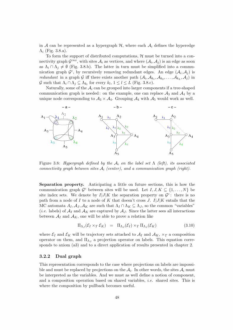
in A can be represented as a hypergraph H, where each Ai defines the hyperedgeΛi (Fig. 3.8.a).
To form the support of distributed computations, H must be turned into a con-nectivity graph Gcnx, with sites Ai as vertices, and where (Ai,Aj) is an edge as soonas Λi ∩ Λj '= ∅ (Fig. 3.8.b). The latter in turn must be simplified into a commu-nication graph Gc, by recursively removing redundant edges. An edge (Ai,Aj) isredundant in a graph G iff there exists another path (Ai,Ak1 ,Ak2, . . . ,AkL ,Aj) inG such that Λi ∩ Λj ⊆ Λkl
for every kl, 1 ≤ l ≤ L (Fig. 3.8.c).Naturally, some of the Ai can be grouped into larger components if a tree-shaped
communication graph is needed : on the example, one can replace A3 and A4 by aunique node corresponding to A3 ×A4. Grouping A4 with A5 would work as well.
'2
4''3
'1 '1
'1 '2
4''3
'2
'1
'2
4''3
'2 '2
'1 '1
A 1
A 3 A 4
A 5
A 2
A 3
A 5
A 4
A 1 A 2
A 3
A 5
A 4
A 1 A 2
− b −− a − − c −
Figure 3.8: Hypergraph defined by the Ai on the label set Λ (left), its associatedconnectivity graph between sites Ai (center), and a communication graph (right).
Separation property. Anticipating a little on future sections, this is how thecommunication graph Gc between sites will be used. Let I, J,K ⊆ {1, . . . ,N} besite index sets. We denote by I|J |K the separation property on Gc : there is nopath from a node of I to a node of K that doesn’t cross J . I|J |K entails that theMC automata AI ,AJ ,AK are such that ΛI ∩ΛK ⊆ ΛJ , so the common “variables”(i.e. labels) of AI and AK are captured by AJ . Since the latter sees all interactionsbetween AI and AK , one will be able to prove a relation like
ΠΛJ (EI ×T EK) = ΠΛJ (EI)×T ΠΛJ (EK) (3.10)
where EI and EK will be trajectory sets attached to AI and AK , ×T a compositionoperator on them, and ΠΛJ a projection operator on labels. This equation corre-sponds to axiom (a3) and to a direct application of results presented in chapter 2.
3.2.2 Dual graph
This representation corresponds to the case where projections on labels are impossi-ble and must be replaced by projections on the Ai. In other words, the sites Ai mustbe interpreted as the variables. And we must as well define a notion of component,and a composition operation based on shared variables, i.e. shared sites. This iswhere the composition by pullback becomes useful.
48

'1
'1
'1
'3 4'
'2
'2
'2
'1
4''3
'1'2'2
'1
'2
4''3
'1
'2
4''3
A 1 A 2
A 3 A 4
A 5
A 1
A 4A 3
A 5
A 2A 1 A 2
A 3 A 4
A 5
A 1 A 2
A 4A 3
A 5
A 1 A 2
A 3 A 4
A 5
A 4
A 1 A 2
A 3
A 5
− a − − b −
− f −
− c − − d −
− e −S1
S5
S2
S3
S4
S1,2
S2,4S1,3
S2,3
S4,5S3,4
S3,5
Figure 3.9: Different ways of defining components as local products of sites Ai.The objective is to capture by such components the constraints that remain in acommunication graph on the Ai, as in Fig. 3.8.c.
49

Let us define components Sk = ×i∈IkAi where Ik ⊆ {1, . . . ,N}. By (3.8), onehas A =
∧k Sk as soon as the Sk cover all the Ai. However, this leaves a lot of
flexibility.Considering that every λ ∈ Λ introduces a constraint on some of the variables
Ai, one can for example take as components the Sλ given by
∀λ ∈ Λ, Iλ = {1 ≤ i ≤ N : λ ∈ Λi} and Sλ = ×i∈IλAi (3.11)
in order to cover the full constraint graph of A. This choice is illustrated in fig-ures 3.9.a and 3.9.b.
This first definition, however, results in quite large components, which can beinefficient for the modular computations described in chapter 2. Another possibilityis thus to consider only pairwise synchronizations and take
∀i, j ∈ {1, . . . ,N}, i < j, Si,j ={
Ai ×Aj if Λi ∩ Λj '= ∅null otherwise (3.12)
A =∧
1≤i<j≤N Si,j is satisfied as soon as every site shares a label with at least onecomponent. This choice is illustrated in Figs. 3.9.c and 3.9.d. In this formulation,the hypergraph induced by components Si,j on nodes Ai reduces to an ordinarygraph : the latter is nothing more than the connectivity graph Gcnx between sites Ai
(compare Fig. 3.9.d to Fig. 3.8.b). To get the connectivity graph between componentsSi,j, we thus have to take the dual of Gcnx.
Apparently, this second definition of components involves a larger number ofsmaller components, and generates a more complex graph. So, at this point, thereis no obvious gain. Recall that some edges in Gcnx are redundant, i.e. describesynchronization constraints between the Ai that are captured by others paths. Sowe reduce the set of Si,j to those that cover a communication graph Gc betweenthe Ai (Fig. 3.9.e and 3.9.f). The remaining components still cover all the Ai, andtheir connectivity graph is still the dual of Gc. This choice not only reduces thenumber of components, but also satisfies nice separation properties (see below). Inparticular, if Gc is a tree, then every communication graph between the selected Si,j
is a tree.
'2'1
'3
A 1
A 2 A 3
S2S1
Figure 3.10: Two components S1 = A1 × A2 and S2 = A1 × A3 that share onlyvariable/site A1, although their interaction is due both to A1 and to the “external”label λ3, not captured by A1.
Separation Property. Anticipating again on future sections, this is how an ex-pression like A =
∧k∈K Sk will be used, assuming that the Sk cover a communication
graph Gc between sites Ai.
50

The first important thing to notice is that the shared variables (= sites) betweentwo Sk do not capture all interactions between these components, so we are notexactly in the setting of chapter 2. Consider the example in Fig. 3.10 : S1 and S2
share only variable/site A1, but they also interact by label λ3 which is not seenby A1. This “external” interaction corresponds to the second line of (3.4) in thedefinition of a pullback, and kills axiom (a3). In other words, it is not possible todirectly translate interactions by shared labels into interactions by shared sites.
Nevertheless, there exists a reasonable range of situations where axiom (a3)holds. For K an index set, let us denote SK =
∧k∈K Sk = AK ′ where K ′ = ∪k∈KIk.
Consider the aggregated components SI = AI′ and SK = AK ′, their shared variablesAJ ′ (with J ′ = I ′ ∩K ′) capture all interactions between SI and SK iff ΛI′ ∩ ΛK ′ ⊆ΛJ ′8. Under this assumption, one will be able to write
ΠAJ′ (EI ∧T EK) = ΠAJ′ (EI) ∧T ΠAJ′ (EK) (3.13)
for EI and EK trajectory sets of SI and SK , respectively, and ∧T a compositionfunction on these trajectory sets.
Lemma 1 Assume components Sk cover a communication graph Gc of the Ai. LetSJ separate SI from SK on their own communication graph, then variables AJ ′
separate AI′ from AK ′ on Gc, and shared variables of SI ∧ SJ and SJ ∧ SK captureall interactions between these aggregated components (Fig. 3.11).
This limited validity range of axiom (a3) is actually sufficient to rederive all resultsof chapter 2, in particular the message passing algorithms.
'3'1 '2
A 5
A 6
A 2A 1 A 4A 3
S1 S2
S5S3
S4
Figure 3.11: Component S4 separates S1 from S2 : its variables see label λ3, respon-sible of a direct interaction between S1 and S2. Consequently, common variables ofS1 ∧ S4 and S4 ∧ S2 capture all interactions between these aggregated components.
3.3 Diagnosis problem
As mentioned in the introduction of this chapter, we concentrate on diagnosis prob-lems, in a wide sense. We first state the problem, then examine two approachesto solve its centralized version, and their ability to be extended into distributedtechniques.
8This situation is referenced as the “structural assumption” in [37, 40].
51

3.3.1 Semantics
So far we have focused on the static structure of systems and didn’t use at all thefact that they are dynamic systems. To introduce the time dimension, we must givea meaning to the notion of trajectory of an LMCA. For a matter of simplicity, weadopt the usual sequential semantics, also called interleaving semantics, and defineruns as sequences of transitions. The next chapters will be based on true concurrencysemantics, where runs are partial orders of events. The latter are more adapted todistributed or modular systems, with sparse interactions and thus a high level ofconcurrency.
As we will see at the end of the chapter, sequential semantics do not fully takeadvantage of the distributed approach to monitoring problems. But their simplicityallows us to present the mathematical skeleton of this framework and the mechanicsof computations, without the technicalities due to partial orders. Once the principlesare established, it will be sufficient to check a few key results to adapt this settingto partial order semantics.
Let A = (S, T, s0,→,χ, I,λ, Λ) be an LMCA. In the sequential semantics (SS),a run (or trajectory) of an LMCA A is modeled as a sequence σ = (t1, t2, . . . , tN ) oftransitions such that •t1 = s0 and t•n = sn = •tn+1, 1 ≤ n ≤ N − 1 (also denoteds0[t1〉 . . . sn−1[tn〉sn[tn+1〉sn+1 . . . [tN 〉sN , and s0[σ〉sN for sequences).
3.3.2 Objectives
Centralized diagnosis, single sensor. Consider an LMCA A, and assume Aproduces a hidden run σ. One gets information about this run by means of a “sensor”that observes part of the transition labels produced by σ. Specifically, we assumethe sensor only collects labels of Λ′ ⊆ Λ, and yields a sequence Ob of observed labels.
The traditional diagnosis problem is stated as follows (see Sampath et al. [95]) :assume a subset T ′ ⊆ T of transitions represents faults that can occur in A. GivenOb, one would like to determine which of the following statements holds :
• a transition of T ′ was fired for sure in σ,
• σ didn’t use any transition of T ′, for sure,
• σ may have fired a transition of T ′, Ob doesn’t allow to decide.
There exist more elaborate forms of the problem, that check whether a complexproperty is satisfied by the hidden run σ given Ob, for example the occurrence of t1followed by two occurrences of t2, etc. (see [61]). They are identical in nature anddo not introduce extra formal difficulties.
A more general version of the diagnosis problem consists in recovering all runsof A that could explain the observed sequence Ob, among which will lie the truehidden run σ. Recovering all runs matching Ob, or estimating the final state of σgiven Ob are almost identical problems. And the latter, called the construction ofan observer for A, is the main building block in the derivation of a diagnoser forA (see next sub-section). So we focus on this version here, that we call the singlesensor centralized diagnosis problem.
52

Centralized diagnosis, several sensors. In the case of a modular system A =A1 × . . . ×AN = S1 ∧ . . . ∧ SK representing a large distributed machine, it is morereasonable to assume several sensors instead of a single one. These sensors can beattached to the Ai, or equivalently to components Sk. We consider the first case forsimplicity, a sensor is attached to each Ai and observes labels of Λ′
i ⊆ Λi (Λ′i = ∅
represents the absence of sensor). When A performs the hidden run σ, the labelsproduced by transitions operating in Ai are collected by sensor i under the form ofa sequence Ob
i . So the observation is now a tuple (O1, . . . , ON ) of sequences, and theobjective remains the same : compute all runs of A that explain these observations.Notice that we lose information with respect to the single sensor case : the exactinterleaving of the different Ob
i is lost.Remark : we assume here that labels attached to transitions in the Ai play a
double role. They are first responsible for transition synchronizations, and they alsocorrespond to observations collected by the sensors. These roles can be separated, forexample by introducing an extra label on transitions to define their visible signature.An alternate solution consists in using a more elaborate synchronization algebrabetween components. In any case, these extensions complexify notations but changevery little in the formal aspects of the problem. So we prefer to keep the simplestformulation.
Distributed diagnosis. The previous task can be extremely complex : one mustconsider all possible interleavings of the Oi, and for each of them the centralizeddiagnosis problem requires to handle a possibly huge system A. The distributed (ormodular) diagnosis approach takes advantage of the interaction structure of A toavoid these difficulties, provided interactions are sparse enough.
In its simplest form, the distributed approach is based on the following ideas :
• a local supervisor Di is attached to each Ai,
• each Di has limited knowledge about A (typically the model of Ai plus someinterface information with the other Aj),
• each Di only knows local observations Obi ,
• the Di compute their local view of the global diagnosis, i.e. they computetrajectories of their component Ai that explain local observations Ob
i and atthe same time are coherent with explanations provided by the other localsupervisors.
The next sections of this chapter will formalize this approach and analyze its prop-erties. Let us just mention that, ideally, a distributed/modular approach to thediagnosis problem must be equivalent to the centralized one, in the sense that thecombination of local results should yield the solution of the (multi-sensor) centralizeddiagnosis problem.
Historically. Considering the evolution of ideas, several intermediate steps wereexplored before the distributed diagnosis problem was stated in the above terms.
53

Early contributions considered first the case of several sensors Obi on the same ma-
chine A, and proposed local supervisors making decisions with the knowledge ofA and Ob
i . These agents would then forward their results to some central super-visor in charge of assembling them according to various simple aggregation rulesor policies [25, 115]. Despite the expensive use of A, there was no reason whysuch decentralized approaches should be equivalent to the centralized one. Whencenotions of decentralized observability, controllability, diagnosability, etc. Anotherapproach considered distributed observations on a modular model, i.e. local agentstaking decisions with the knowledge of Ai and Ob
i , and making assumptions on theinteractions with neighboring components. Once again, local agents would forwardtheir results to a central supervisor in charge of assembling them, now with the aimof obtaining equivalence with the centralized diagnosis [8, 88]. The last step wasthen to get rid of the central supervisor, which meant 1/ distributing its job underthe form of a cooperation between local agents, and more essentially 2/ abandoningthe objective of global solutions available somewhere, now replaced by a distributedknowledge [103].
3.3.3 The diagnoser approach
Given an LMCA A and a subset of visible labels Λ′ ⊆ Λ, an observer for A isa deterministic automaton DA, taking labels of Λ′ as input, and which states aresubsets of states of A. When A performs a hidden run σ and outputs the labelsequence Ob ∈ Λ′!, DA fed with Ob reaches a unique state that lists all possiblestates where A could be, given Ob (Fig. 3.12).
!
!
!"
((
b
c
d!
!
!
!"
{a,c}
{b,c,d}
{c}
{a,c,d}
{d}
"a
Figure 3.12: An automaton (left) and its observer (right) for visible labels Λ′ ={α,β}.
DA can be obtained easily in two steps [15] :
1. an epsilon-reduction, that replaces each state of A by its invisible reach (statesreachable through invisible transitions), followed by
2. a determinization, that aggregates states reachable by the same transitionlabel.
To obtain a diagnoser for A, let us consider a trivial two state automaton Bthat stays at state “green” as long as transitions of T \ T ′ are fired, and otherwisemoves from “green” to “red” and stays there forever. The synchronous productA×B (synchronization on transition names) replicates A with an augmented state,to memorize the firing of a fault transition. The observer of A×B yields a diagnoserfor A : when all states of DA×B are green, the answer will be that no faulty transition
54

occurred, etc. Notice that by a straightforward extension, one can actually test anyregular property on runs of A, i.e. properties that can be expressed under the formof an automaton B [61].
There is a simple case where this construction extends to modular LMCA. As-sume A = A1×A2, the observer DA1×A2 factorizes as DA1×DA2 when shared labelsare visible on both sides, i.e. when Λ1∩Λ2 = Λ′
1∩Λ′2. Indeed, under this assumption
the epsilon-reductions only remove local transitions, and the product of determinis-tic automata remains deterministic. Interestingly, the visibility of interactions wasoften assumed in publications related to distributed diagnosis [25], but it doesn’tseem its importance for the modularity of the diagnoser has been noticed. The re-sult is not mentioned in [22] for example, although it is fundamental for the modulardiagnosability tests developed in this work. And, similarly, the same assumption ishidden in [54, 55]. The extension of the modularity property of the diagnoser to thecase of invisible synchronization events remains an open question. The result seemsto hold with weaker assumptions, but if modular diagnosers always exist, it is likelythat one could derive from them a joint observability/diagnosability test, in the caseof distributed observations, which is shown in [105] to be undecidable.
To summarize, diagnosers offer the advantage to be computable off-line : theactual observed sequence is not needed. Diagnosers are “recursive” in nature, in thesense that they can process observations on the fly, and at low cost. On the side ofdrawbacks lies the problem of size, of course, since they are designed to process anypossible sequence of observations. And the modularity of diagnosers doesn’t holdfor most interesting cases, where component interactions are hidden.
3.4 Distributed diagnosis : the language approach
Distributed computations based on languages were independently proposed by RongSu in [102, 103]. This approach probably forms the simplest framework for themethodology we propose in this document, so we re-express it here in our formalism.We then adapt it to perform computations on runs of a composite system.
3.4.1 Diagnosis in terms of languages
Centralized diagnosis. Consider a labeled automaton A = (S, T, s0,→,λ, Λ)producing a hidden run σ that is observed through the label set Λ′ ⊆ Λ. This yieldsthe observed sequence Ob = ΠΛ′(σ) where ΠΛ′ is the natural projection on labelsof Λ′. Let us denote by L(A) ⊆ T ! the language of A, i.e. the set of projectionsΠΛ(σ) where σ ranges over all runs of A. In this section, we consider a simplifiedversion of the diagnosis problem : we wish to recover all words of L(A) that yieldOb when projected on Λ′. We call this the diagnosis of Ob. It is given by
D = L(A) ∩Π−1Λ′ (Ob) = L(A)×L Ob (3.14)
where ×L is of course the parallel product of languages.
55

Several sensors. Let us now consider a modular automaton A = A1 × . . .×AN ,with Ai = (Si, Ti, s0
i ,→i,λi, Λi), and distributed observations Obi of the hidden run σ,
Obi = ΠΛ′
i(σ) where Λ′
i ⊆ Λi. As explained in the previous section, distributed obser-vations mean a loss of information : one only knows that there exists an interleavingof the Ob
i that corresponds to the hidden run σ. So let’s take
Ob = Ob1 ×L . . .×L Ob
N (3.15)
as observation, which computes all compatible interleavings of theObi . The diagnosis
is again given by D = L(A)×L Ob, i.e. words of L(A) compatible with at least oneinterleaving of the Ob
i . Of course, both Ob and L(A) are generally large, so inpractice there is no hope to solve the problem in that way.
Distributed diagnosis. Let us consider instead the structure of A. From A =A1 × . . . ×AN we derive
L(A) = L(A1)×L . . .×L L(AN) (3.16)
Inserting (3.16) and (3.15) into (3.14) yields
D = [L(A1)×L Ob1]×L . . .×L [L(AN )×L Ob
N ] (3.17)
where L(Ai)×L Obi ! Di is a local diagnosis, i.e. the set of words of component Ai
that explain local observations Obi .
We can now apply the results of chapter 2 : variables are the labels in Λ, andcomponents are languages on theses labels (see the language systems section 2.1.2).D has a product form, where factors Di are components operating on labels Λi. SoD admits a minimal product covering
D = D′1 ×L . . .×L D′
N with D′i ! ΠΛi(D) (3.18)
The D′i correspond to the local views of the global diagnosis : they contain words of
L(Ai) that both explain local observations Obi and that are compatible with local
explanations in all other components.As explained in chapter 2, the desired D′
i can be computed in a modular mannerwithout computing D itself, given the fact that the parallel product of languages ×L
and projections ΠΛ′ on subsets of labels satisfy axioms (a1)-(a4). The support ofmodular computations is a communication graph Gc between components Ai, in the“direct graph” viewpoint (Fig. 3.8.c), because projections are defined with respect tolabels. If Gc is a tree, convergence to the D′
i is reached in finite time. Otherwise, onecan either group components to recover a tree, or simply ignore cycles and apply aturbo procedure. Since language systems are involutive, turbo algorithms are knownto converge to a unique point (at least for the weak topology) and provide reasonable(upper) approximations D′′
i of the D′i : D′
i ⊆ D′′i ⊆ Di and D = D′′
1 ×L . . .×L D′′N .
3.4.2 Diagnosis in terms of trajectories
Let us come back to our original problem : determining runs of A that would explainthe sequence Ob of observed labels.
56

By post-processing. Let L(A) denote the “language” of A, now expressed interms of sequences of transitions instead of sequences of labels. Obviously, the new“diagnosis” we are looking for is the inverse projection of D on L(A) :
D ! L(A) ∩Π−1Λ′ (Ob) = L(A) ∩Π−1
Λ (D) (3.19)
where Π−1Λ′ yields sequences of transitions. In the same way, when A = A1×. . .×AN
the local views of the global diagnosis are as well clearly given by reverse projectionsof the D′
i on the L(Ai)
D′i = L(Ai) ∩Π−1
Λi(D′
i) (3.20)
However, to prepare for the techniques we develop in the sequel, it is worth deter-mining directly D and the D′
i by computations on trajectory sets.
By direct computation. We first refine the notion of product ×L, to adapt it totrajectory sets. Consider two LMCA A1,A2 and their product A1×A2. There existnatural projections Πi : L(A1×A2) → L(Ai) : they simply replace transitions (t1, t2)by ti, and erase the latter when ti = &si . Let T1,T2 be subsets of L(A1), L(A2),respectively, we define their label-based product by
T1 ×L T2 = Π−11 (T1) ∩Π−1
2 (T2) (3.21)
Naturally, when A = A1 × . . .×AN this product preserves
L(A) = L(A1)×L . . .×L L(AN ) (3.22)
For a matter of homogeneity, we could encode Ob as a labeled sequence of tran-sitions (as we will do in the sequel) in order to compute its product with L(A). Forthe sake of simplicity, let us rather extend ×L to sequences of labels, which allowsus to write :
D = L(A)×L Ob (3.23)
To express our problem in the setting of chapter 2, we must now define systems,variables and projections of systems on these variables. We take Vmax = {1, . . . ,N}6Λ, so compared to the previous section, we add site names to the variable set. Thesystems we consider are formed by
• words w of Λ∗, and by
• labeled sequences of tuples (ti)i∈I for some I ⊆ {1, . . . ,N}, that form validruns of AI . We denote them by (σ, ΛI) to keep track of the label set attachedto the run σ of AI .
So we have two types of sequences, but the systems we define below will containsequences of a single type. The composition operation ×L applies to both types ofsequences.
57

Let us now come to projections. For J ⊆ {1, . . . ,N} and Λ′ ⊆ Λ we must defineΠJ+Λ′ of the two objects above. On a word w of Λ∗, we take
ΠJ+Λ′(w) ! ΠΛ′(w) (3.24)
which erases labels not in Λ′. And on a run (σ, ΛI) of AI
ΠJ+Λ′(σ, ΛI) !{
(ΠI∩J(σ), ΛI ∩ Λ′) if I ∩ J '= ∅ΠΛ′(σ) otherwise (3.25)
So the run σ becomes a “pure” label sequence when no site of I is common to J .With this encoding, ×L and Π satisfy axioms (a1)-(a4). Systems L(AI) operate
on variables I 6 ΛI and are involutive. The diagnosis D is given by
D = [L(A1)×L Ob1]×L . . .×L [L(AN )×L Ob
N ]! D1 ×L . . .×L DN (3.26)
and admits the minimal product form
D = D′1 ×L . . .×L D′
N with D′i ! Πi,Λi(D) (3.27)
Once again, this reduction problem can be computed by MPA, where messagesare exchanged between sites Ai (or disjoint groups of sites AI). The propertiesare the same as for language systems. Nevertheless, observe a very nice feature ofthis setting : each variable i is private to site Ai, i.e. sites only share labels. Sothe messages exchanged between sites are sequences of labels, while sites actuallycompute on sequences of transitions.
3.4.3 Extensions and drawbacks
The two approaches above, by language systems or by trajectory systems, can beextended in several ways.
Recursivity. First of all, they can be made recursive. Assume the Obi are not
given once for all, but correspond to growing sequences of observations, that weencode as Ob
i (t) : Obi (t) ⊆ Ob
i (t+1), t ≥ 0. As explained at the end of section 2.2.2,message passing algorithms applied to changing local diagnoses Di(t) = L(Ai) ×L
Obi (t) remain valid and preserve their convergence properties, provided observations
sequences stabilize. And the Di(t) can of course be computed recursively.
Distributed optimization. Secondly, one could associate cost functions to wordsof L(Ai) or to local runs of the L(Ai), and adopt a (min,+) setting to define thecomposition. Message passing algorithms would then compute (or approximate)the word (resp. the run) of minimal cost in L(A) (resp. in L(A)) explaining allobservations.
58

Drawbacks. Both aspects can of course be combined, so apparently we alreadyhave the appropriate framework to deal with networks of dynamic systems and wecould stop here. However, these approaches based on sets of sequences suffer fromtwo serious drawbacks.
1. The first drawback relates to the size of the local diagnoses Di(t) or Di(t) :they grow rapidly with the length of the observation sequence Ob
i (t), becauseof branchings occurring in Ai. So even if one performs modular computations,the “modules” themselves become enormous with time. We therefore need tofind a compact manner to encode sets of runs of a component Ai. This isprecisely the objective of the next section.
2. The second drawback is a consequence of the sequential semantics, inappro-priate for concurrent systems. It multiplies the number of runs by computinguseless interleavings. This effect appears in particular in product operationswhen few labels are common. Consider the extreme case of two componentsA1,A2 that do not interact at all (no shared label), and a trajectory σi of nevents in each of these components. There exist 2n different interleavings ofthese two runsσ1 and σ2, that will be considered as different runs of the jointsystem A1 × A2. Even with a compact way of encoding local diagnoses Di,combinatorial explosions remain due to the fact that concurrency is not han-dled properly (see section 3.7). The next chapters will address this difficultyby recasting all results in a true concurrency semantics.
3.5 Trajectory sets in the sequential semantics
The mathematical skeleton of the previous section gives an accurate view of thestructure of computations that we perform in the sequel. The main change that weintroduce now relates to the objects on which these operations apply : we replacelanguages by more complex structures that encode sets of runs in a compact manner.
3.5.1 Trellis automaton
We had already defined the category A, formed by labeled multi-clock automataassociated to a notion of morphism. A guiding property when one defines morphismsis that they must preserve runs :
Lemma 2 Let φ : A1 → A2 be an LMCA morphism, and let σ1 be a run of A1,then σ2 = φ(σ1) is a run of A2.
Naturally, φ(σ1) is defined by the recursion φ(σ1|t1) = φ(σ1)|φ(t1) if φ(t1) '= &, andφ(σ1|t1) = φ(σ1) otherwise.
We now focus on the representation of sets of trajectories for a given LMCA. Todo so, we introduce a sub-category of LMCA : A is said to be a trellis automaton(TA) when
1. the graph of A, determined by →, is directed and acyclic, or equivalently →∗
defines a partial order on nodes of A (i.e. states and transitions),
59

2. this partial order is well founded : ∀x ∈ S ∪T, | {x′ ∈ S ∪T : x′ →∗ x} | < ∞,
3. s0 is the unique minimum of this partial order : ∀x ∈ S ∪ T, | {x′ ∈ S ∪ T :x′ '= x, x′ →∗ x} | = 0 ⇔ x = s0.
As a consequence, in any run σ = (t1, . . . , tn) of a TA, all transitions ti are different.In the sequel, states of a TA are called conditions (denoted by c ∈ C instead ofs ∈ S), and transitions are called events (denoted by e ∈ E instead of t ∈ T )9.
A trellis automaton κ = (C ′, E′,→′, c0,χ′, I,λ′, Λ) is called a configuration whenit is composed of a single sequence of events : ∀c ∈ C ′, |•c| ≤ 1 and |c•| ≤ 1. Wewill say that κ is a “configuration of T ” when this configuration is a sub-TA of T .Changing slightly notations, we now identify runs of T with its configurations.
Multi-clock function. To events of T we associate a vector-clock value definedby the function
∀e ∈ E, he : I → Ni :→ he(i) = 1Ii∈χ(e)
(3.28)
So an event counts 1 for component i iff it influences this component. This definitionleads to the notion of height of a condition c in a configuration κ of T . Assume κcorresponds to the sequence of events (e1, e2, . . . , en, . . .) and goes through conditionc immediately after en, we define
Hκ(c) !N∑
n=1
hen (3.29)
For every component index i ∈ I, Hκ(c) thus counts the number of events associatedto component i and before c in run κ, whence the name “multi-clock function.” Itobviously relates to vector-clocks of Mattern [84] and Fidge [50].
A trellis automaton T is correctly folded iff ∀c ∈ C and for any pair κ,κ′ ofconfigurations of T containing c, one has Hκ(c) = Hκ′(c). In other words, only se-quences of events with the same multi-clock value can merge at the same condition c(see Fig. 3.13).
From now, we only consider correctly folded trellis automata ; they form thesubcategory T of A. In a (correctly folded) TA T , one can of course write H(c)instead of Hκ(c).
3.5.2 Time-unfolding of an automaton
Let A ∈ A, T ∈ T, and let f : T → A be a morphism. The pair (T , f) is a trellisprocess (TP) of A iff
1. f is a folding of T onto A (i.e. a total function on states and transitions),9These names come from the definition of branching processes, that describe runs of Petri nets
in the true concurrency semantics.
60

t1 t2
t6t4t3 t5
t8 t10t9
t1 t2
t6t4t3 t5
t8t7 t7t9 t10
a
b
d e
g
c
f
ih
a
b
d e
g
c
f
ih
Figure 3.13: Two trellis automata, with two components : thin arrows represent tran-sitions associated to component 1, and thick arrows those associated to component 2.The TA on the left is correctly folded, the other one isn’t : the merge at h is illegal.
2. T satisfies the parsimony criterion :
∀e, e′ ∈ E, [ •e = •e′, f(e) = f(e′) ] ⇒ e = e′ (3.30)
3. T is maximally folded :
∀c, c′ ∈ C, [H(c) = H(c′), f(c) = f(c′) ] ⇒ c = c′ (3.31)
f can be viewed as a labeling of events of T by transitions of A. This definition thusensures that if κ is a configuration of T , then (κ, f|κ) encodes a run of A (point 1).Moreover, thanks to the parsimony criterion,
Lemma 3 Let (T , f) and (κ, f ′) be trellis processes of A, and assume κ is a config-uration. There exists at most one injective morphism φ : κ→ T such that f ′ = f ◦φ.
This states that a run of A is represented at most once in a trellis process of A. Asa direct consequence,
Lemma 4 Two trellis processes of A representing the same trajectories of A areactually isomorphic.
So trellis processes provide the compact structure we are looking for to describe setsof runs of an LMCA.
Notation: for the sake of simplicity, we often omit mentioning the folding f in arun (κ, f) or a trellis process (T , f) of A, and simply talk about κ or T .
Let A = (S, T, s0,→,χ, I,λ, Λ) be an LMCA. One can build a trellis process(T , f) of A by the following recursion :
Procedure 1
1. Initialization : C = {c0}, f(c0) = s0, E = ∅
2. Recursion : for c ∈ C and t ∈ T such that f(c) = •t,if !e ∈ E such that •e = c and f(e) = t, then
(a) create e ∈ E, set •e = c, f(e) = t, χ′(e) = χ(t) and λ′(e) = λ(t),
61

(b) create c′ ∈ C, set •c′ = e and f(c′) = t•,
(c) if ∃c′′ ∈ C with f(c′′) = f(c′) and H(c′′) = H(c′), then merge c′ and c′′.
The three conditions of the definition are satisfied by construction, and clearly anytrellis process of A can be obtained in that way, with a suitable guiding of events toconnect.
On the basis of the above unfolding procedure, one can recursively define theunion of two or more trellis processes of A, which produces another TP of A. Noticeright now that the union T1 ∪ T2 may contain configurations that were not presentin any of the Ti, but that nevertheless remain valid runs of A. We come back onthis point later.
Lemma 5 Let (T , f) be a trellis process of A, then T is isomorphic to the unionof its configurations (κi, fi). As a consequence, two trellis processes of A that haveisomorphic configurations are isomorphic.
Let us define the prefix relation T1 ; T2 between TP by the fact that T2 containsmore configurations of A than T1, or equivalently that there exists an injectivemorphism φ : T1 → T2. The above lemmas lead to the following important result :
Theorem 7 Given an LMCA A, there exists a unique maximal trellis process ofA for the prefix relation. We denote it (Ust
A , fA) and call it the sequential time-unfolding of A (ST-unfolding or STU for short).
The proof is simple : Define (UstA , fA) as the union of all trajectories (κ, f) of A.
Unicity is obvious from lemma 5, which also shows that the STU contains all trellisprocesses of A.
stat
es
timet4 t4
t2
t1 t1 t1 t1
t2 t2 t2
t3t3t3t5t5
. . .
a a a a a
bbbb
c c c
t1
t5t2
t3t4
a
b c
Figure 3.14: An ordinary automaton A(left) and its sequential time-unfolding UstA
(right). The folding fA is represented by state and transition names close to condi-tions and events.
Fig. 3.14 illustrates the notions of trellis process and sequential time-unfoldingon an ordinary automaton, i.e. an LMCA with |I| = 1. The STU, commonly calledthe trellis of an automaton in digital communications, is the support of the Viterbialgorithm, for example in the maximum likelihood decoding of noisy bits whentransmissions are protected by a convolutional error correcting codes. Trellises alsoform the implicit support of the Bellman equation, in optimal control problems. Soonly the multi-clock aspects are new.
62

Observe that the size of an ordinary trellis grows linearly with its length. Witha multi-clock criterion to determine merge points, the number of possible mergesdecreases and one obtains a larger structure, with growing width. But it remainssmaller than the simple unfolding of A, that unfolds both time and conflicts (orchoices) and yields a decision tree. And the latter is in turn smaller than thelanguage of A.
Relation between trellis processes and sub-languages. The time-unfoldingof A encodes all possible runs of A, or equivalently all the language of A. Butrecall that a union of configurations of A generally results in a TP that containsmore runs. So what are the sub-languages of A that can be represented by a trellisprocess ?
Let (κ1, f1) and (κ2, f2) be two runs of A, with c0i [κi〉ci. They are said to be
H-equivalent, denoted by κ1 <H κ2, iff f1(c1) = f2(c2) and Hκ1 = Hκ2, i.e. iff theyhave same length, and start and finish at identical states of A. A sub-language L ofA is said to be suffix-closed iff
∀κ = κ1κ′1 ∈ L, ∀κ2 ∈ L, κ1 <H κ2 ⇒ κ2κ
′1 ∈ L (3.32)
Lemma 6 Let L be a sub-language of A, L can be encoded as a trellis process of Aiff it is prefix- and suffix-closed.
The prefix-closure requirement is a little embarrassing, but can be easily dis-carded. Let us enrich the definition of a trellis process (T , f) with a stop functionSt : C → {0, 1} on conditions. We then associate to (T , f, St) the sub-language Lof A formed by configurations (κ, f) of T that finish on a stop point : c0[κ〉c andSt(c) = 1. Then
Proposition 7 There is a one to one correspondence between stopped trellis pro-cesses of A and sub-languages L of A that satisfy
∀κ = κ1κ′1 ∈ L, ∀κ2 ∈ L, κ1 <H κ2 ⇒ κ1 ∈ L ∧ κ2κ
′1 ∈ L (3.33)
(3.33) expresses both suffix-closure and a weaker form of prefix-closure.Notice however that the above limitations in the expressive power of trellis pro-
cesses will not prevent modular computations and diagnosis based on them.
3.5.3 Variations around the height function
The multi-clock function that governs merge points of trajectories is somehow arbi-trary and can be generalized, provided its vector nature is preserved. So far, eachevent affecting component i was counting for 1 in the clock of that component. Onecan easily relax this assumption.
For example, let (E ,=, ε) be a set provided with an internal composition law =,and ε as neutral element. Let us attach to each LMCA A a function that assigns aheight vector to all transitions : ∀t ∈ T, ht : I → E such that i '∈ χ(t) ⇒ ht(i) = ε,so the height of t is neutral for component i when t doesn’t affect it. Naturally, weprovide these new LMCA with height preserving morphisms.
63

To define the height of a condition c in a configuration κ, we simply combinethese height values : for κ terminating at c and consisting of events (e1, . . . , en), wetake Hκ(c) = he1 = . . .= hen (component-wise composition of vectors).
One can of course choose (E ,=, ε) in order to have monotonic clocks, but thisis not necessary : circuits apparently don’t bother the theory10. They can even beuseful to avoid unfolding specific parts of a system. Assume for example that onewishes to count events that produce a label in Λ′ ⊂ Λ and ignore all other events.This can be done by he = ε whenever λ(e) '∈ Λ′. So silent loops are not unfoldedin the time-unfolding of A. We refer the reader to [46, 47] for the interest of thisproperty in diagnosis applications. Notice that the idea of not unfolding silent loopswas introduced by Lamperti and Zanella [72].
By contrast, it is extremely important to preserve the vector nature of a heightfunction. Abandoning this structure means breaking the universal property statedin theorem 8 below, and consequently blocking the distributed diagnosis approachbased on it. We come back on the necessity of vector clocks at the end of the chapter(see also [46, 47]).
As a remark in passing, let us mention that one can easily design a strictlyincreasing height function that would allow no merge point at all. For example aheight function that stores all the past of a condition. In this case, the sequentialtime-unfolding of A coincides with its ordinary unfolding, also called a decision-tree.Consequently, all results we state on sequential time unfoldings remain valid forordinary unfoldings.
3.5.4 Categorical properties
The awkward function χ : T → I introduced in the definition of LMCA could haveappeared as a useless decoration up to now. This feature is actually necessary toobtain the following result.
UAst
A
%
E
!& fA
T A
Figure 3.15: Universal property of the STU of A.
Theorem 8 (Universal property) Let A ∈ A be an LMCA, let T ∈ T be a trellisprocess and φ : T → A a morphism, there exists a unique morphism ψ : T → Ust
Asuch that φ = fA ◦ ψ.
Theorem 8 essentially expresses that Ust(A) describes all runs of A, and describesthem only once (this explains the necessity of being “maximally folded” for a trellisprocesses).
10This is only a conjecture at this point, verified on a set of examples. For a rigorous proof, onewould have to redefine trellis processes to allow circuits, under the constraint of a height function.And then check the preservation of theorems 7 and 8.
64

U
AutomataTrellis automatastU
Figure 3.16: Two functors relating A and T, that form an adjunction.
When designing a structure to encode runs of A, as soon as its universal propertyis satisfied, some classical category theory arguments are triggered and lead to veryuseful results. We sketch this reasoning below.
T being a sub-category of A, there exists an inclusion functor F =⊆ : T → A.Conversely, the ST-unfolding operation on LMCA defines a functor G = Ust : A →T. By “functor,” we mean that Ust applies also to morphisms and satisfies Ust(f ◦g) = Ust(f)◦Ust(g). The fact that G = Ust is a functor is a direct consequence of theuniversal property associated to any Ust
A . The latter also entails that (F,G) forms apair of adjoint functors (see [81] chapter 4, in particular theorem 2.iv, p. 81). As theright adjoint of the pair, G preserves categorical limits, and so preserves products(see [81] chapter 5.5, in particular theorem 1, p. 114). In other words, one has
∀A1,A2 ∈ A, Ust(A1 ×A2) = Ust(A1)×T Ust(A2) (3.34)
where ×T denotes the categorical product in T. By contrast with×, the product in Tnot only synchronizes events with shared labels, but also preserves the partial order-ing of the resulting structure. It must be understood as an operation synchronizingtrajectories instead of automata.
*
T
*
f1f2
’ ’
f
t2t1t3
b c
c
at’1t1
t’3t3
t2t’2
t’4ccb’ cc’
bb’ cc’
aa’
t’2t’4
t’4
t’2
t’1t’3
a’
b’c’
c’c’
c’b’
A1U ( )st A2U ( )stx A2U ( )stA1U ( )st
t’1t1 t2t’2
t’3t3 t’4c
bb’
cb’
cc’aa’t’3 t’4
t’2t’1 b’ c’# )
"!a’t3
t1 t2b ca#
! "
A1 x A2A1 A2
$1 $2
$1 $2
Figure 3.17: Top : two LMCA and their product. Bottom : the corresponding STU(on this example they coincide with classical unfoldings). The 7 morphisms relatingthese LMCA form a commutative diagram.
Fig.3.17 illustrates this property. The top line represents two LMCA A1 andA2, with their product (in the center), and the associated canonical projectionsπi : A1 × A2 → Ai. A1 and A2 share labels {α,β, γ} but δ is private to A2. The
65

bottom line represents the corresponding sequential time-unfoldings, together withtheir foldings (materialized by state and transition names close to conditions andevents). The STU Ust
A1×A2is isomorphic to the product Ust(A1)×T Ust(A2), which
has canonical projections π′i : Ust(A1) ×T Ust(A2) → Ust(Ai) to its factors. The7 morphisms mentioned on the picture form two commutative squares, thanks totheorem 8. Observe that Ust
A1×A2has two conditions pointing to the same state
(c, c′) of A1 × A2 : they correspond to different multi-clock values, and thus can’tbe merged. By doing so, one would get a structure isomorphic to A1 × A2, andthere wouldn’t exist a morphism π′1 anymore. In other words, that would kill (3.34),which shows the importance of separate counting of time in the various componentsof an LMCA.
The adjoint pair (F,G), where F corresponds to an inclusion, is called a core-flection. Since additionally one has ∀T ∈ T, T < Ust(T ) (read “isomorphic to”),one can actually define the product ×T by
∀T1,T2 ∈ T, T1 ×T T2 < Ust(T1)×T Ust(T2) = Ust(T1 × T2) (3.35)
This last relation has an important practical consequence : by combining Proce-dure 1, computing ST-unfoldings, to the definition of the product in A, one gets arecursive algorithm to compute the product in T.
Finally, just like products, pullbacks are also categorical limits. So the reasoningsabove apply in the same way and one has
∀A0,A1,A2 ∈ A, Ust(A1A0∧ A2) = Ust(A1)
Ust(A0)∧T Ust(A2) (3.36)
where the pullback ∧T in the sub-category T of trellis automata is defined by
∀T0,T1,T2 ∈ T, T1T0∧T T2 < Ust(T1)
Ust(T0)∧T Ust(T2) = Ust(T1
T0∧ T2) (3.37)
And once again, the combination of Procedure 1 with the definition of ∧ gives arecursive algorithm to compute pullbacks in T .
3.6 Distributed diagnosis : the trellis approach
The properties we have obtained on trellis processes are now very close to those oflanguage systems, so can we really compute with trellises ?
In this section, we come back to our diagnosis application with these new tools.We follow the steps of section 3.4 to highlight the formal similarities, but also thetechnical extensions that are needed. As we will see, the major difference is that wecan’t use of projections on subsets of labels. So projections will now be defined withrespect to sites Ai, and we will adopt the dual graph viewpoint of section 3.2.2.
3.6.1 Centralized diagnosis, single sensor
The setting doesn’t change : A performs a hidden run κ whose labels are observedunder the form of sequence Ob. The latter can be encoded as a trivial trellis au-tomaton, formed of a single sequence, i.e. Ob is a configuration. We are still looking
66

for runs of A that would explain Ob. Since we have a product on trellis processes,(3.14) becomes
D = Ust(A)×T Ob (3.38)
A few comments on this equation.It is meaningless to unfold A and then compute the product. This formal re-
lation must be translated in practice into a recursive algorithm : one computesthe unfolding of A guided by observations Ob, which is closer to the expressionD = Ust(A ×Ob) given by (3.35).
Secondly, by contrast with (3.14) or (3.23), D defined in (3.38) contains runsof A that explain only a prefix of Ob, and not the entire Ob. This effect can becorrected easily : it suffices to use stopped trellis processes, as defined at the end ofsection 3.5.2. They form a sub-category of stopped automata, assuming morphismsthat preserve stop points. The theory is identical to what has been presented above,so we omit this detail, for the sake of simplicity, and assume that (3.38) does yieldruns of A that entirely explain Ob. We refer the reader to [46, 47] and [48] fordetails.
3.6.2 Centralized diagnosis, several sensors
When A = A1 × . . . × AN and Ai has Λi as label set, assume again that labels ofthe hidden run κ are collected by independent sensors attached to the sites Ai. Thesensor on Ai collects labels of Λ′
i ⊆ Λi and produces the configuration Obi . One can
again assemble these observations by
Ob = Ob1 ×T . . .×T Ob
N (3.39)
which computes all possible interleavings of the sequences Obi , and then apply (3.38).
The latter will then amount to an unfolding of A guided by a complex trellis au-tomaton Ob, instead of a sequence. This is feasible, but of course very inefficient,because of the complexity of both A and Ob. Fig. 3.18 illustrates this point : thetwo sequences of observations share a single label, β. The result of the product ismuch more complex than its factors, because it develops all concurrency diamonds.So we are rather looking for diagnosis methods that operate on factorized forms,and avoid expanding large products. This is in fact the heart of the approaches weadvocate in this document.
3.6.3 Distributed diagnosis
Before addressing the distributed diagnosis issue, we must introduce the notion ofprojection of a trellis process on sets of sites Ai.
Projections. The site index set {1, . . . ,N} becomes our variable set Vmax, andwe have to define projections ΠI for I ⊆ Vmax. For simplicity, we will use notationΠI instead of ΠAI , when there is no ambiguity.
67

"
#
##
#
!
!
!
#
#
!
!
aa’
de’ab’
ac’ ce’
dd’bb’
ba’
bc’ cd’
O1 x TO2
O1a b c d" !! ! "1* ={ , }’
O2a’ b’ c’ d’ e’" ###
" #* ={ , }2’b
b
b b
Figure 3.18: The product of two configurations compute all possible interleavings ofthese sequences, which results in many concurrency diamonds.
Let K,L ⊆ {1, . . . ,N} be site index sets, and assume K ⊆ L. From the productform Ust(AL) = Ust(AK)×T Ust(AL\K) we know there exists a canonical projection
ΠL,K : Ust(AL)→ Ust(AK) (3.40)
Every trellis process of AL is a prefix of Ust(AL), so ΠL,K applies to TP of AL andyields TP of AK .
When K '⊆ L, we define ΠL,K as ΠL,K∩L, and since the starting point is gen-erally unambiguous, we simply write ΠK instead of ΠL,K . By associativity of ×T ,projections satisfy ΠK ◦ΠL = ΠK∩L, which corresponds to axiom (a1).
In practice, projections ΠK are quite easy to implement. Consider for exampleFig. 3.18 : it suffices to collapse nodes related by events that do not belong to thesites we want to preserve. The result is almost a trellis process of the selected sites,excepted that it violates the parsimony criterion : isomorphic events may branchout of a given node. Therefore a simple trimming operation is also necessary.
Objective. The central result that we invoke now is the factorization property ofthe sequential time-unfolding of A. Given A = A1 × . . .×AN , (3.34) becomes
Ust(A) = Ust(A1)×T . . .×T Ust(AN ) (3.41)
and thus the diagnosis admits the factorized form
D = [Ust(A1)×T Ob1]×T . . .×T [Ust(AN )×T Ob
N ] (3.42)
In this equation, each Di = Ust(Ai) ×T Obi is a local diagnosis : it selects runs of
site Ai that explain the local observations Obi . The distributed diagnosis problem
simply amounts to computing the minimal product covering of D, i.e. to computingthe Ti = ΠAi(D), which yields
D = [T1 ×T Ob1]×T . . .×T [TN ×T Ob
N ] (3.43)
Equivalently, one could also compute the D′i = ΠAi×Ob
i(D) = Ti ×T Ob
i that alsosatisfy D = D′
1 ×T . . . ×T D′N . The latter are called the “reduced” local diagnoses.
68

In the sequel, we don’t distinguish these two reduction problems, that are identicalin nature and can be solved in the same manner, with the same complexity.
Apparently, we are thus in a well known land, as explored in chapter 2. Inreality, there is a major difference with section 3.4.2, due to the fact that we don’thave projections on label sets.
New shape of computations. Our objective is to recover the D′j by means of
modular computations. Consider two LMCA A1,A2 that share labels Λ1,2 ! Λ1∩Λ2,see (3.44). Let T = T1×T T2 be a trellis process of A1×A2, and let us try to replicatethe modular computations of section 3.4.2 in order to compute the minimal productcovering of T . One would have to project T1 on Λ1,2, in order to form a messageM1,2 = ΠΛ1,2(T1) that would be some sort of label structure. The latter would thenbe combined by a special product ×L to T2 and would produce T ′
2 = T2 ×L M1,2.And symmetrically to obtain T ′
1 .
A1Λ1,2 A2 (3.44)
As we have seen, this approach works on simple structures like sets of sequences,but, unfortunately, projections of trellis processes on label sets are hard to define :By simply erasing the events of a trellis process that do not carry a visible label, onewould kill the trellis structure. Even worse, this can create circuits, and produce astructure containing fake sequences of visible events11.
So to transfer information from one side to the other, we bypass this undefinedlabel structure and use a trick, based on more familiar operations : We first combineT1 and T2, and project the result on A2 to form the message : M1,2 = ΠA2(T1×T T2).One can conclude by T ′
2 = M1,2 ∧T T2. This computation trick looks like a tautologyon such a trivial example. But it makes sense to propagate information when oneimagines a third site A3 beyond A2. As we show below, modular computations areactually based on this idea.
Expression of A with pullbacks. Since we can’t project on labels, we are boundto use projections on sites or sets of sites Ai. So the Ai become our variables, andto comply with the formalism of chapter 2, we must express our systems in termsof shared variables, i.e. in terms of shared sites.
We know that A can be reformulated as A = S1 ∧ . . . ∧ SM , where componentsSj are defined by Sj = AIj = ×i∈Ij Ai and cover all the Ai, i.e. ∪1≤j≤M Ij ={1, . . . ,N}. By (3.36), one has
Ust(A) = Ust(S1) ∧T . . . ∧T Ust(SM ) (3.45)
and similarly
D = [Ust(S1)×T ObI1 ] ∧T . . . ∧T [Ust(SM )×T Ob
IM]
! D1 ∧T . . . ∧T DM (3.46)11It is not excluded however that more clever height functions would solve this difficulty. But
this is still a research topic.
69

where the local diagnoses Dj = Ust(Sj) ×T ObIj
are now computed on componentsinstead of sites. The expression above assumes that every local diagnosis Dj in-corporates by Ob
Ijthe observations on all sites AIj covered by component Sj. In
reality, the duplication of observations Obi is unnecessary : it is sufficient to “dis-
tribute” them on components Sj in such a way that they all appear at least once.However, taking all Ob
Ijto compute Dj has the advantage to “maximally reduce”
Ust(Sj) before message exchanges start.The distributed diagnosis problem now amounts to computing the Tj = ΠSj (D),
or equivalently the D′j = ΠSj×Ob
Ij(D) = Tj ×T Ob
Ij, that form the minimal “pullback
covering” of D :
D = [T1 ×T ObI1 ] ∧T . . . ∧T [TNM ×T Ob
IM]
= D′1 ∧T . . . ∧T D′
M (3.47)
Naturally, the minimal product covering can be obtained by further projecting theD′
j on the individual sites they represent.
Separation theorem. To relate things to chapter 2 in a clear manner, we nowhave a variable set Vmax = {1, . . . ,N}, trellis processes TI as systems, projectionsΠI and the composition operator ∧T . So we are in the setting of the dual graphrepresentation (section 3.2.2). But at this point, the central axiom (a3) is missing...The reason is that the interactions in A = A1 × . . . ×AN are due to shared labels,and we need to express them in terms of shared sites. When one computes AI ∧AK,the shared sites AI∩K do not necessarily capture all interactions between AI andAK : shared labels ΛI ∩ ΛK may not all lie within ΛI∩K (see Fig. 3.10 and thediscussions in section 3.2.2).
Nevertheless, one has the following property
Theorem 9 Let I,K ⊆ {1, . . . ,N}, and take J = I ∩K. Let TI ,TK be trellis pro-cesses of AI ,AK respectively, and assume that shared sites AJ capture all interactionlabels between AI and AK , i.e. ΛI ∩ ΛK ⊆ ΛJ . Then
ΠJ(TI ∧T TK) = ΠJ(TI) ∧T ΠJ(TK) (3.48)
This weaker form of axiom (a3) is actually sufficient to derive modular computations.Propagation and merge equations now take the following form :
Proposition 8 Let I, J,K ⊆ {1, . . . ,N}, and let TI ,TJ ,TK be trellis processes ofAI ,AJ ,AK respectively. If ΛI ∩ ΛK ⊆ ΛJ , denoted I|J |K, then
ΠJ(TI ∧T TJ ∧T TK) = ΠJ(TI ∧T TJ) ∧T ΠJ(TJ ∧T TK) (3.49)ΠI(TI ∧T TJ ∧T TK) = ΠI [TI ∧T ΠJ(TJ ∧T TK)] (3.50)
Comparing these equations to the “true” ones (2.8) and (2.10), the reader will noticethat proposition 8 simply implements the “trick” described at (3.44).
70

Support graph of computations. So far, no choice was made to decomposeA into a pullback of components and obtain (3.45). We now exploit this degreeof freedom, that was already discussed in section 3.2.2, dedicated to dual graphrepresentations.
Let us define components Sk in such a way that they cover a communicationgraph Gc between sites Ai (Fig. 3.19). Then form a communication graph Gc′ be-tween these components. The latter forms the support of computations. Indeed,on graph Gc′, the separation property holds, which means that theorem 9 applies,so propagations and merges of proposition 8 are legal and the MPA leads us to thedesired reduced components S ′
j .
'1
'2
4''3
'1
'1 '2
'2
4''3
A 4
A 1 A 2
A 3
A 5
− a −
A 1
A 4A 3
A 5
A 2
− c −
A 1 A 2
A 3 A 4
A 5
− b −
A 3
A 2
− d −
S1
S3
S2
S2
S1
S3
Figure 3.19: From left to right : label constraints between sites Ai, a communicationgraph Gc of the Ai, a definition of components Sj covering Gc, and a connectivitygraph between components Sj .
We didn’t mention sites corresponding to measurements, i.e. the Oi. Theyactually play no role in the structure of interactions, even if the Oi observe sharedlabels. Indeed, each Oi is separated from all other sites (including measurementsites) by site Ai. So introducing the Oi in Fig. 3.19.b simply amounts to putting anedge between each Ai and the associated Oi ; all edges between the Oi, if any, aredotted (i.e. redundant). Moreover, since the Oi correspond to observations collectedon a true run of A, the projections ΠOi(D) necessarily yield Oi. In summary,measurements can just be ignored in the graphical representations.
Involutivity. It is not hard to check that trellis processes form involutive systems :for TI a TP of AI , one has TI ∧T ΠJ(TI) = TI . So we are in the nice situation whereturbo procedures converge, if the support graph of computations is not a tree. Theprogressive reduction performed by MPA (theorem 4) and the local extendibilityproperty of the limit (theorem 3) are thus granted.
3.7 Towards true concurrency semantics
This section comes back to the multi-clock aspects, in order to (try to) convince thereader of its necessity for modular computations.
Consider the two LMCA A1,A2 of Fig. 3.20. They synchronize on labels {α,β, γ},
71

and transitions t5 and t′4 are private to A1 and A2 respectively. Fig. 3.21 depicts twotrellis processes T1,T2 of these LMCA, together with their “products” for differentchoices of height functions. The first product (3rd TP on the figure) correspondsto T1 ×T T2 in the multi-clock setting : time is counted independently in each com-ponent, which prevents the merge of the two conditions labeled (c, c′), since theycorrespond to different values of the vector clock.
t’1 t’3
t’2 t’4
a’
c’
! #
b’"
t3t2
t1
t5
a
d
#
c
b"
!
A 1 A 2
Figure 3.20: Two labeled multi-clock automata, sharing labels {α,β, γ}.
Assume that one would decide to abandon vector clocks and choose to use aglobal counting of time in the definition of trellis processes. The “product” T1×T T2
would then result in the rightmost TP of Fig. 3.21 where the two conditions labeled(c, c′) are now merged, since they both have two events in their past. Projectingback the result on A1 (by erasing events of A2) underlines the bad properties ofthis construction : this projection yields a “trellis process” isomorphic to A1. So theresult is not any more a correctly folded trellis process of A1. But worse than that,this projection introduces the extra run a[t3〉c[t5〉d that was not present initially inthe factor T1. So there is little hope that modular computations based on this notionof trellis process would produce correct results.
t1t’1 t3t’3
t2t’2 t’4
t5
aa’
bb’ cb’
cc’ cc’
dc’
t3 #t1
t2
t5
a
d
c
b!
"
ct’1 t’3
t’2 t’4
a’
c’
! #
b’"
t1t’1 t3t’3
t’4
t5cc’
dc’
t2t’2
aa’
bb’ cb’
T1 T2T1 T T2 T1 T T2
multi!clock folding single clock folding
Figure 3.21: Two trellis processes of the previous LMCA, their correct product, anda product based on a global notion of time.
To explain the bad properties of this “single-clock product” T = T1 ×scT T2 by
the more formal aspects of our construction, notice that T doesn’t correspond to
72

a categorical product. There doesn’t exist morphisms from T to its two factors T1
and T2 (actually there is no morphism to T1). In other words, considering T as avalid trellis process would violate the universal property stated in theorem 8 on T1.There exists a morphism from T to A1, that doesn’t decomposes into a morphismto T1 followed by the folding of T1 into A1.
t5
t5 t’4t’4t’2t2
t3 t’3t’1t1
b b’
a’a
c b’
c’ c’ d c’c
d
t5
t3 t’3t’1t1
t’2t2 t’4 t5
b
a’a
c
c
d
b’
dc’
Figure 3.22: Unfolding and time-unfolding of A1 ×A2 of Fig. 3.20.
Since one is bound to the use of vector clocks, this means that the relevant notionof time for distributed systems is itself distributed [84, 50]. Rather than a universallinear time, one has local notions of time, plus synchronizations on special events.Pushing further this idea, it makes sense to develop a setting where transitionsthemselves would have local effects. This suggests to use a distributed notion ofstate, rather than global states, and adopt true concurrency semantics.
Consider for example A1 and A2 of Fig. 3.20. These new semantics will lead to anew notion of product for A1×A2, as well as new notions of unfolding U(A1×A2)(Fig. 3.22 left) and of time-unfolding U t(A1×A2) (Fig. 3.22, right). On this example,the product A1 ×A2 would actually look like the latter : simply merge the subnetsbelow the two conditions labeled c.
These new representations of sets of runs, U(A) and U t(A), display explicitlythe concurrency of events : for example the concurrent firings of t4 and t5. In thissetting, the product of two systems that have no interaction will amount to their jux-taposition. That will avoid the useless computation of concurrency diamonds, andresult in even more compact data structures to encode sets of runs. The next chap-ter examines computations based on unfoldings, in the true concurrency semantics,and chapter 5 does the same with trellises, or time-unfoldings.
As an extra motivation to move to true concurrency semantics, let us illustrate alast drawback of sequential semantics. We have seen that vector clocks are necessaryto modular computations. Nevertheless, they have very unpleasant side effects : insome cases, there may exist a drift between clocks of two components. In particularwhen these components have concurrent behaviors (i.e. local transitions). In termsof trellis processes, this results in very large structures, as illustrated in Fig. 3.23.These phenomena suggest not to recommend the approach of this chapter, and useinstead true concurrency semantics, that will erase such weird behaviors.
73

bb’
aa’
ab’ ba’
ba’ ba’
ba’ab’
ab’
aa’aa’
aa’ aa’
ab’
bb’bb’
bb’
t2
t2
t3
t3
t1t’1t’4 t’4
aa’
ab’
ba’
bb’
a
b
a
bt1
t2
t3
t’4 t’1!t1!
t2
t2
t3
t1!
t1!
t1!
a’
b’
a’
b’
a’
t’1!
t’1!
t’4
t’4
t3
t3
a
b
b a
a
b
a’
b’
Figure 3.23: Top : two LMCA A1,A2 that share label α, and their product A1×A2.Bottom : the STU Ust(A1), Ust(A2) and their product Ust(A1 ×A2).
74

3.8 Summary
We have proposed a methodology to deal with distributed systems by means of dis-tributed or modular algorithms, with the diagnosis problem as guiding application.To do so, we first introduced the notion of network of automata. Mathematically,one can easily derive modular diagnosis algorithms based on component languages :they take the form of message passing algorithms, originally derived for Bayesiannetworks. The keystone of the construction is a factorization property on sets ofruns of the global system, just like in Bayesian networks the factorization propertyof the global likelihood function is the key to fast algorithms.
Nevertheless, computing with component languages demands important storagecapabilities, which is not suited to practical applications, in particular if we aim aton-line monitoring algorithms. So we have proposed a more compact way of encodingsets of runs, by means of trellis processes. A well known notion in different researchcommunities, that has been adapted here to networks of automata. This adaptationrequired to introduce the concept of multi-clock, i.e. to keep track of componentswhen they are assembled into networks. Without this concept, it seems difficult toobtain the factorization property on trellis processes of a compound system, which isessential to modular computations. As soon as this property is derived, which is mosteasily done with category theory arguments, the mathematical framework developedfor languages applies to trellis processes, up to some technical modifications.
Introducing vector clocks in distributed systems is a first step to a correct mod-eling of concurrent behaviors. This is what we do in the next chapters, moving fromsequential semantics to true concurrency semantics. We will show that the mathe-matical skeleton of this chapter still applies, up to some technical extensions, andthat we can obtain even more compact descriptions of sets of runs.
Related work
The diagnoser approach has been first investigated in [95], with a focus on diagnos-ability issues. Diagnosability means that a bounded number of observations afterthe occurrence of a fault is sufficient to detect the failure. This amounts to check-ing the absence of ambiguous circuits in the diagnoser, i.e. (in the formalism ofsection 3.3.3) circuits of the observer of A × B that contain state estimates of thetwo kinds, green and red. Issues appearing with distributed observations and/orsystems have been soon considered. The protocol-based approach of [25], for exam-ple, assumes distributed observations on separate components, but global diagnosersare used at each sensor, and the focus is on the information they should exchangeto merge their estimates. By contrast, [21, 22] introduce a true distributed ap-proach, where local diagnosers are based on a local model. Similar results are alsoderived in [54, 55], with a slightly different model : components are defined as Petrinets instead of automata. In both cases, component interactions are assumed tobe visible, which guarantees that the diagnoser/observer of the global model has aproduct form, and thus enables modular solutions. Unfortunately, the problem isnot so much analyzed from this angle, which hides the important phenomena thatmake things work. For example the fact that, when interactions are observed, no
75

matter which interleaving of the observed sequences is chosen in Fig. 3.18, the sameestimated states are obtained.
The literature related to distributed diagnosis is vast and diverse. Several ap-proaches make use of message passing (or belief propagation) algorithms, in relationto the topology of the supervised system, but assume no dynamics in the compo-nents. For example [89] deploys MPA on failure trees, and [97, 98] use dependencygraphs between the elementary functions that compose a network. All these modelsare stochastic but static.
As already mentioned, the closest contributions to chapter 3 are due to Su andWonham [102, 103]. They do use networks of dynamic systems, where each compo-nent is specified as a language. The approach is purely algebraic : no randomizationis assumed, by contrast with the previous ones. Let us also mention the contribu-tions of Pencole [88], or Baroni et al. [8]. They both model a distributed system as anetwork of communicating automata, and consider the distributed on-line construc-tion of a “diagnoser” (sic), i.e. a system whose runs are exactly the explanationsto the distributed observations. Although the idea is to progressively assemble the“local diagnosers,” by a product, this is not properly a message passing solution :there is no notion of projection. But strategies are deployed in [88] to avoid buildinguseless parts in the recursive composition of local diagnosers. Interestingly, the ideaof not unfolding silent loops is present in these two contributions.
Finally, let us mention the very original chronicle approach [28, 30, 49]. Bycontrast with the previous ones, it doesn’t look for an explanation to all alarms orsymptoms. It rather operates as a collection of filters that extract relevant patternsof observations in a sequence. These patterns are specified as partial orders of labels,related by time constraints. There exist both fast chronicle recognition algorithms,and learning algorithms. Another difference with model-based approaches is thatthe expert knowledge must come afterwards, to evaluate the relevance of learnedchronicles and to associate them to a failure “diagnosis.” There exist techniques,however, to merge chronicles with topology models [5, 56].
76

Chapter 4
True concurrency semantics
So far, we have defined a distributed system as a network of components, with local-ized interactions. We have shown that some monitoring problems, like (maximumlikelihood) trajectory estimation, that we called the diagnosis problem, could besolved in a distributed manner. The modular/distributed resolution method ex-ploits the factorization property of sets of runs, under the various forms where theseruns can be described. In the sequential semantics, run sets can be encoded either
• as sets of sequences (of labels or transitions),
• as branching processes or decision trees, or
• as trellis processes,
which establishes a hierarchy in terms of compactness. Moving to true concurrencysemantics, this hierarchy remains. It is also remarkable that the algebraic structureof distributed computations is preserved. Extra gains are obtained in terms ofcompactness of the objects we handle, at the price of a little more technicality inthe proof of the key results.
This chapter presents the interest of branching processes, and the new featuresthey introduce in the distributed diagnosis problem. Chapter 5 will make one morestep and study the counterpart of trellis processes.
4.1 Networks of automata as asynchronous systems
The previous chapter introduced a notion of component, somehow artificially, intothe ordinary definition of an automaton : in A = (S, T,→, s0,χ, I,λ, Λ), I is anindex set that gives names to components, and the function χ : T → 2I defineson which components every transition t ∈ T “operates.” Although components areformally added by the product of (labeled) multi-clock automata, the compositionnevertheless results in an automaton. Fig. 4.1 illustrates this idea, in a Petri-net-likerepresentation of automata.
This formalism suffers from several drawbacks, some of which have been illus-trated at the end of the previous chapter. Let us underline two of them.
77

t2 " t4 # ( ,t )4b*
*(t , )2 c
*(t , )2 d
( ,t )4a*1 3(t ,t )
1t ! t3 !
a
b
c
d
"
"
##!
ac bc
bdad
Figure 4.1: Two LMCA (left) that share only label α, and their product (right).
Numbers of states and transitions are multiplied by the composition, and inparticular each private transition of one factor is duplicated n times, where n is thennumber of states of the other factor. So we explicitly represent the fact that oneLMCA is waiting when the other performs a private transition (see the duplicationsof t2 and t4 in the example).
Secondly, runs of a product LMCA A1×A2 are almost bound to be sequences ofevents : the fact that the reset transitions t2 and t4 are concurrent is not exploited.So one distinguishes (t1, t3)(t2, &d)(&a, t4) from (t1, t3)(&b, t4)(t2, &c), whereas it wouldbe preferable to write (t1, t3)t2t4 and (t1, t3)t4t2, and even consider these two runs asequivalent, since t2 and t4 can be permuted without altering the final state ofA1×A2.
The objective of this chapter is precisely to avoid the redundancy introduced bythe sequential semantics, and explicitly take advantage of the concurrency betweenevents. We’ll take as definition of a run not a sequence of transitions, but an equiva-lence class of sequences, where equivalence means “identical up to the permutation oftwo successive concurrent events.” In the example above, { (t1, t3)t2t4 , (t1, t3)t4t2 }will be considered as a single run. In other words, sequences will be replaced byMazurkiewicz traces [27].
t2 " t4 #1 3(t ,t )
t2 " t4 #1t ! t3 !
a
b
c
d
a
b
c
d
!
Figure 4.2: Two labeled automata (left) combined into a safe Petri net (right).
To do so, a natural step consists in replacing automata by asynchronous systems.This is simply obtained by changing the notion of composition : in substance, wetake the disjoint union of states (instead of the product), and glue transitions thatcarry identical labels, in all possible ways, to form joint transitions. Private transi-tions remain unchanged. As illustrated in Fig. 4.2, this yields a Petri net : we nowhave several “tokens” to identify a global state of the system. Firing (t1, t3) movessimultaneously the two tokens to b and d, after what they can return to their original
78

places independently. Observe that the number of tokens remains constant : thisillustrates the fact that we now have two components, or equivalently two (local)state variables, instead of one.
There exist several formalisms to define and handle such systems. Our origi-nal contributions [37, 40] chose to emphasize the presence of several state variable,which lead to the notion of tile system (see also the introduction, section 1.3). Al-ternatively, one could simply consider safe Petri nets. But since we need to preservethe notion of component, or of variable, the latter must be slightly enriched. Wetherefore introduce the notion of multi-clock net (MCN).
This chapter is organized as the previous one : we first define the category of(labeled) multi-clock nets, and their composition. We then provide them with a no-tion of trajectory, in the true concurrency semantics. As for multi-clock automata,a crucial problem is the compact representation of sets of trajectories. We focushere on the notions of branching process and unfolding of a MCN, the natural coun-terparts of the sequential trellis process and the sequential time-unfolding, exceptedthat merges are not allowed. So these objects are more on the side of decision trees.It is shown that one can actually compute with them, pretty much like with sequen-tial trellis processes. But specific difficulties of the true concurrency semantics blurthe nice algebraic setting of the previous chapter. We show that computations mustactually be performed with more complex objects, that we call augmented branchingprocesses.
4.2 Multi-clock nets and their composition
4.2.1 A category of multi-clock nets
Petri net. An ordinary Petri net is a 4-tuple N = (P, T,→,M0) where P, T arerespectively the place and transition sets1, and →⊆ (P × T ) ∪ (T × P ) is the flowrelation relating places and transitions2. M0 : P → N is a finite multi-set on Prepresenting the initial marking of the net, i.e. the number of tokens that eachplace initially holds. Given a node x ∈ P ∪ T , •x and x• stand for pre- and post-sets, i.e. the immediate predecessors and successors of x in →. By contrast withthe previous chapter, these sets are not any more constrained to be singletons.
A transition t ∈ T is enabled (or activated ) in a marking M , denoted by M [t〉,iff ∀p ∈ •t,M(p) > 0. Firing t from M yields the new marking M ′ = M − •t + t•,which we denote by M [t〉M ′. M is a reachable marking iff there exists a sequenceσ = (t1, t2, . . . , tn) of transitions (or a run) and intermediate markings such thatM0[t1〉M1[t2〉M2 . . . [tN 〉MN = M , abbreviated into M0[σ〉M . We limit ourselvesto safe nets, i.e. nets for which places hold at most one token in any reachablemarking. We thus identify markings to subsets of P , and M0 to P 0 ⊂ P .
Multi-clock net. A multi-clock net (MCN), or net for short, is a tuple N =(P, T,→, P 0, ν) where
1We do not require that P and T be finite.2We assume each place is related to one transition at least, and each transition has at least one
input place and one output place.
79

1. (P, T,→, P 0) is an ordinary safe net,
2. ν : P → P 0 defines a partition on places, and the restriction ν|P 0 is theidentity ; we denote by p the equivalence class ν−1(ν(p)) of a place p,
3. ∀t ∈ T , ν is injective on •t and on t•, and ν(•t) = ν(t•).
This definition deserves some comments.Observe first that every transition satisfies |•t| = |t•|. So the number of tokens
remains constant in a MCN. Moreover, let M ⊆ P be a reachable marking of N ,one has ν|M is bijective. In other words, let p ∈ P 0, at any time there is exactly oneplace in ν−1(p) holding a token3.
Secondly, consider N|p, the restriction of N to places of p, p ∈ P . N|p is anautomaton, i.e. a Petri net where a single place holds a token at any time, as inFig. 4.1. Therefore, a multi-clock net can be regarded as a synchronous product ofautomata, as illustrated in Fig. 4.2.
Relating this formalism to the previous chapter, P 0 now replaces the index set Ito name components, and the χ function on transitions is replaced by ν on places.So a transition t operates on components ν(•t) = ν(t•) instead of χ(t). By abuseof vocabulary, we will sometimes consider p as the state variable of component N|p(more rigorously, it corresponds to the set of possible values of this state variable).
Naturally, a labeled multi-clock net (LMCN) is a MCN enriched with a labelingfunction on transitions : N = (P, T,→, P 0, ν,λ, Λ), with λ : T → Λ.
i i’
t 1 t 2 t 3
t 4 t’4
a b c d
e f g h
t2 t3
i
t 4
c’
h
d’c
g’g
Figure 4.3: A typical morphism between two multi-clock nets, indicated by dashedarrows. In the left MCN, ν1 defines the partition {a, e}, {b, f}, {c, g}, {d, h, i, i′} onplaces.
Morphism. To turn the collection of multi-clock nets into a category, we needthe extra notion of morphism between nets. Let N1,N2 be two MCN, with Ni =(Pi, Ti,→i, P 0
i , νi), i = 1, 2. A morphism φ from N1 to N2 is defined as a pair(φP ,φT ) where
3Notice that it is always possible to turn a safe net N into a multi-clock net with essentially thesame behavior, simply by adding to each place of N a complementary place. So multi-clock netsare almost equivalent to safe nets.
80

1. φT is a partial function from T1 to T2, and φP a relation between P1 and P2,
2. P 02 = φP (P 0
1 ) and φopP : P 0
2 → P 01 is a total function, where φop
P denotes theopposite relation to φP ,
3. if p1 φP p2 then the restrictions φT : •p1 → •p2 and φT : p•1 → p•2 are totalfunctions,
4. if t2 = φT (t1) then the restrictions φopP : •t2 → •t1 and φop
P : t•2 → t•1 are totalfunctions,
5. φP preserves the partitioning of places : ∀(p1, p2) ∈ P1 × P2, p1 φP p2 ⇒ν1(p1)φP ν2(p2)
Notice that points 3 and 4 entail that the pair (φP ,φT ) preserves the flow relation(on its domain of definition), and so morphisms will preserve runs, which is the firstproperty one expects from them. It may look surprising that φP is a relation andnot a partial function. This generalization allows φP to duplicate places, which isnecessary to the existence of a categorical product (recall that this duplication abilitywas also present in MCA morphisms). In conjunction with the last requirement, onecan actually show that
Lemma 7 Let φ : N1 → N2 be a morphism of MCNs, such that every automatonNi|p has a single connected component, then φ erases or duplicates state variables(or components) as a whole, just like MCA morphisms (see Fig. 4.3). Specifically,one has
a. the inverse image by φ of a class of ν2 is included in a class of ν1 ;
b. given a class of ν1, φ is either defined on all elements of this class, or on noneof them ;
c. when a place p1 ∈ P1 is duplicated by φ, i.e. related to (elements of) severalclasses of ν2, each place in p1 is duplicated in the same way, i.e. related to thesame classes.
Finally, for labeled MCN Ni = (Pi, Ti,→i, P 0i , νi,λi, Λi), i = 1, 2, the definition
of a morphism φ : N1 → N2 must be reinforced by extra requirements (that rephrasethose of labeled MCA) :
6. Λ2 ⊆ Λ1, i.e. φ reduces the label set,
7. Dom(φT ) = λ−11 (Λ2), i.e. φ is defined on transitions carrying a shared label,
and only on them,
8. if φT (t1) = t2 '= & then λ1(t1) = λ2(t2), i.e. φ preserves labels on its domainof definition Dom(φT ).
We denote by Nets the category having the LMC nets as objects, and the abovemorphisms as arrows. By abuse of notations, we simply write φ instead of φS or φT ,and φ(X) to denote places in relation with at least one place in X.
81

4.2.2 Composition by product and pullback
Product. Let N1,N2 be two LMCN, their product N1×N2 is defined as the triple(N ,ψ1,ψ2) where N = (P, T,→, P 0, ν,λ, Λ) is a net and ψi : N → Ni a morphism,such that
1. P = {(p1, &) : p1 ∈ P1} ∪ {(&, p2) : p2 ∈ P2} ;ψ1(p1, &) = p1 and ψ1(&, p2) = & (i.e. undefined), and symmetrically for ψ2,
2. P 0 = ψ−11 (P 0
1 ) ∪ ψ−12 (P 0
2 ),
3. T = Ts ∪ Tp where
Ts = {(t1, t2) ∈ T1 × T2 : λ1(t1) = λ2(t2)} (4.1)Tp = {(t1, &) : t1 ∈ T1, λ1(t1) ∈ Λ1 \ Λ2}
∪ {(&, t2) : t2 ∈ T2, λ2(t2) ∈ Λ2 \ Λ1} (4.2)
and ψi(t1, t2) = ti if ti '= & and is undefined otherwise,
4. → is defined by •(t1, t2) = ψ−11 (•t1)∪ψ−1
2 (•t2), assuming •& = ∅, and similarlyfor (t1, t2)•,
5. Λ = Λ1 ∪ Λ2 and λ follows accordingly,
6. ν is simply the union of partitions ν1 and ν2.
In a product, each component preserves its places by the disjoint union in (1),and components are added (6). As for LMCA, transitions carrying a shared labelsynchronize (4.1), provided they find a partner, while those carrying a private labelremain unchanged (4.2). Notice that private transitions are not duplicated, bycontrast with LMCA. See Fig. 4.4 for a simple example.
b
a d
e fc
g
t3 t2 t1 t4 t5 t6t’4t’1! " "!
Figure 4.4: Product of three nets, each one with a single component. On this simpleexample, the product amounts to gluing transitions with identical labels.
Proposition 9 × is the categorical product in Nets , i.e. the universal propertystated in proposition 5 for LMC automata holds also for LMC nets.
See [112] for a proof in the unlabeled case, which easily specializes.
82

Pullback. The composition by pullback, i.e. via a shared component, can alsobe defined for LMC nets, and it enjoys the same properties as for LMC automata.The general definition is a little complex [43], so we focus on the more intuitive casewhere N1,N2 are related to their interface N0 by partial functions fi : Ni → N0
instead of general morphisms. The construction resembles very much the one of theproduct : it actually coincides with it outside the domains of f1 and f2. N and themorphisms ψi : N → Ni are given by
1. P = Pc ∪ Pp where
Pc = {(p1, p2) : f1(p1) = f2(p2) = p0 ∈ P0} (4.3)Pp = {(p1, &) : f1(p1) = &} ∪{ (&, p2) : f2(p2) = &} (4.4)
ψi(p1, p2) = pi if pi '= & and undefined otherwise,
2. P 0 = ψ−11 (P 0
1 ) ∪ ψ−12 (P 0
2 ),
3. T = Tc ∪ Ts ∪ Tp where
Tc = {(t1, t2) : f1(t1) = f2(t2) = t0 ∈ T0} (4.5)Ts = {(t1, t2) : f1(t1) = & = f2(t2), λ1(t1) = λ2(t2)} (4.6)Tp = {(t1, &) : f1(t1) = &, λ1(t1) ∈ Λ1 \ Λ2}
∪ {(&, t2) : f2(t2) = &, λ2(t2) ∈ Λ2 \ Λ1} (4.7)
and ψi(t1, t2) = ti if ti '= & and is undefined otherwise,
4. → is defined by •(t1, t2) = ψ−11 (•t1)∪ψ−1
2 (•t2), assuming •& = ∅, and similarlyfor (t1, t2)•,
5. Λ = Λ1 ∪ Λ2 and λ follows accordingly,
6. ν is the union of partitions ν1 and ν2 : they coincide on the common places ofψi(Pc).
The novelty appears in the special treatment of common places (4.3) and commontransitions (4.5).
Proposition 10 The composition by ∧ corresponds to a pullback in the categoryNets .
The proof of the universal property of the pullback, see (3.3) and Fig. 3.4, can befound in [43]. So we are on solid ground, and derivations of the previous chapterbased on category theory arguments still hold : we only changed objects. In par-ticular, the relations between × and ∧ expressed in proposition 6 remain valid forLMC nets, as illustrated in Fig. 4.5.
83

N1 N0 N2
f1 f2
b
a
c
g d
f
g
ce
c
g
t3 t2 t4t1 t5 t6t1 t4t1 t4! " "! ! "
Figure 4.5: Two nets, that share a common component. The limit of this diagram(pullback) results in the net of Fig. 4.4.
4.2.3 Graphs associated to a multi-clock system
The situation is exactly as for labeled multi-clock automata (section 3.2). We startfrom a net N defined as a product N = N1 × . . . × NN , and want to representgraphically the internal interactions of N . The objective is of course to prepare theground for distributed/modular algorithms.
There are essentially two ways to do so : either by a direct graph representation(the common resources, or variables, are the shared labels) or by a dual graphrepresentation (the common resources are the sites Ni). Here, we will mostly usethe latter : the choice is indeed governed by the type of projections we use in thesequel, either projections on label sets, or projections on sites. It is not excludedthat the branching processes we introduce below for modular computations couldadmit projections on label sets ; we are actually working on the topic. But so farthis theory is not available, and we can only project on (sets of) sites. This choicethus imposes to base computations on pullbacks, as in section 3.6.3.
In summary, thanks to proposition 6 and property (3.8) expressed on nets, wecan decompose N as
N =∧
j∈J
Sj with Sj = ×i∈IjNi (4.8)
assuming components Sj cover a communication graph between sites Ni (Figs. 3.9-eand 3.9-f).
4.3 Trajectory sets in the true concurrency semantics
This section defines the notion of trajectory of a net, in the true concurrency se-mantics, and proposes means to represent sets of runs and compute with them. Inthe previous chapter, a set of runs of an LMCA could be understood and handledin four different manners : as a set of label sequences (sub-language), a set of transi-tion sequences (a richer notion of sub-language), and more compactly as a branchingprocess, or as a trellis processes. The same ideas would apply here in the true con-currency semantics. We skip the first one, limited to labels, and directly move toruns expressed as traces on transitions, that we will represent as configurations. And
84

since configurations will appear as specific cases of branching processes, we directlymove to the latter and show how to compute with these objects. Trellis processesform the body of the next chapter.
4.3.1 Unfolding of a net
Occurrence net. The LMC net O = (C,E,→, C0, ν,λ, Λ) is a (labeled multi-clock) occurrence net (LMCON, or ON for short) iff it satisfies :
1. C0 = {c ∈ C : •c = ∅},
2. the causality relation →∗, irreflexive transitive closure of→, is a partial order,and ∀x ∈ C ∪ E, [x] ! {x} ∪ {y ∈ C ∪ E : y →∗ x} is finite,
3. ∀c ∈ C, |•c| ≤ 1,
4. the conflict relation # defined by the two properties below is irreflexive :
(a) ∀e, e′ ∈ E, [e '= e′, •e ∩ •e′ '= ∅] ⇒ e#e′,
(b) ∀x, x′ ∈ C ∪ E, [∃e, e′ ∈ E, e#e′, e →∗ x, e′ →∗ x′] ⇒ x#x′.
The change in notations accounts for the usual terminology of conditions, insteadof places, and events, instead of transitions. In an LMCON, “time” is unfolded, asindicated by (2). A condition can be marked by a unique event (3). By contrast,it may enable several events, which corresponds to a conflict situation. This createsa branching in the net, and the corresponding branches will never meet each otheragain (4). So conflicts are also unfolded. See Fig. 4.6, center, for an example.
Configuration. LMCONs are generally introduced to represent runs of a net inthe so-called true concurrency semantics. To do so, we need extra elements ofterminology about ONs. Two nodes x, x′ ∈ C∪E are said to be concurrent , denotedby x⊥⊥x′, iff neither x#x′ nor x→∗ x′ nor x′ →∗ x holds. A co-set is a set of pairwiseconcurrent conditions, and a cut is a maximal co-set for the inclusion. Finally, aconfiguration is a sub-net κ of C ∪E which is conflict-free, causally closed (i.e. left-closed for →∗), and such that ∀e ∈ E, e ∈ κ ⇒ e• ⊆ κ. By convention we assumeconfigurations also contain initial conditions C0. See Fig. 4.6, right, for an example.
One immediately notices the one-to-one correspondence between configurationsof an occurrence net and possible runs of that net, i.e. possible circulations oftokens. Specifically, a configuration must be read as a partial order of events. InFig. 4.6 (right), the firing of t1 precedes or is a cause to the firing of t5, just liket3, however, the ordering of t1 and t3 is not specified. So they can fire in anyorder. Every linear extension of the partial order defined by a configuration yieldsa valid firing sequence on its events. In that sense, a configuration represents anequivalence class of sequences, or a trace [27]. This is precisely where the trueconcurrency semantics allows to save with respect to the previous chapter : uselessinterleavings of concurrent events are not represented, and a single partial orderreplaces numerous sequences.
85

t 1 t 2
a
t3 t 4
b
t5 t 5 t 5 t 5
ba ba baba
c c d d
t5
ba
t1 t 3
c d
a b
t5 t5 t 5
ba baba
t2 t4
c d
t5
t2 t 3 t 4
dc
a b
t1
Figure 4.6: An LMC net N (left), a branching process O of that net (center) and aconfiguration κ in O (right), corresponding to a run of N . The folding of O into Nis represented by transition and place names attached to events and conditions.
LMC occurrence nets, equipped with morphisms of LMC nets, form the sub-category Occ of Nets . Observe that in this category, morphisms can only erase (notcreate) causality or conflict relations between two nodes. Concurrency relations arepreserved, and configurations are mapped to configurations.
Branching process. The pair (O, f), where f : O → N is a morphism, is saidto be a (labeled multi-clock) branching process (LMCBP or BP for short) of net Niff [31]
1. f is a total function on O, also named a folding of O,
2. ∀e, e′ ∈ E, [•e = •e′, f(e) = f(e′)] ⇒ e = e′.
In other words, f labels all events and conditions of O by transitions and placesof the net N (see Fig. 4.6). f being a morphism, this labeling actually turns aconfiguration κ of O into a run of the net N . The parsimony condition 2. ensuresthat any run of N that is represented in O appears only once, or is represented bya unique configuration.
There exist similarities between the branching processes of LMC nets definedabove for nets and the sequential branching processes defined for LMC automata.In particular the categorical architectures are identical, so the main results can betransported here. We briefly review them.
First of all, there exists a simple and intuitive algorithm to build a branchingprocess (O, f) of net N , that looks very much like Procedure 1 (without the mergeof conditions). We briefly mention it below4, since it forms the basis of severaloperations we use in the sequel.
Procedure 2
• Initialization :4This recursive construction is explicit in [110] as well as in [35], where new events and places are
named by a backward pointer technique. It also appears in the definition of “canonical branchingprocesses” in [31].
86

– Create |P 0| conditions in C0, and define a bijection f : C0 → P 0.– Set C = C0, E = ∅ and →= ∅.
• Recursion :
– Let X be a co-set of C and t ∈ T a transition of N such that f(X) = •t.– If there doesn’t exist an event e in E with •e = X and f(e) = t,
∗ create a new event e in E with •e = X and f(e) = t,∗ then create a subset Y of |t•| new conditions in C, set Y = e•,
and extend f to have the bijection f : Y → t•.
The partition ν of conditions in O is of course inherited from the partition of placesin N , as well as the labeling λ of events.
Lemmas 3, 4 and 5 remain valid for branching processes of a net N , and oneeasily modifies the recursion of Procedure 2 to compute the union of branchingprocesses of A, which leads to the notion of unfolding.
Unfolding. A prefix O′ of an occurrence net O is defined as a sub-net of Owhich is causally closed, contains the initial marking (or equivalently all minimalconditions), and such that ∀e ∈ E, e ∈ O′ implies e• ⊆ O′. So a configuration of Ois a conflict-free prefix of O. The prefix relation is denoted by O′ ; O.
Theorem 10 Given a net N , there exists a unique maximal branching process ofN for the prefix relation. It is called the unfolding of N . We denote it by U(N ),or UN for short, and its corresponding folding by fN : UN → N .
A proof of this theorem can be found in Winskel’s works [110] or in Engelfriet’s [31].The unfolding is of course obtained as the unique stationary point of Procedure 2,
and its configurations yield all possible runs of N .
Expressive power of branching processes. We had mentioned in the previouschapter that not all sub-languages L of an LMCA A could be represented as asequential trellis (or branching) process. In the same way :
Lemma 8 Let L be a set of configurations of N . L can be represented as a BP(O, f) of N iff
∀κ ∈ L, κ′ ; κ ⇒ κ′ ∈ L∀κ1,κ2 ∈ L, κ1 ∪ κ2 is a configuration ⇒ κ1 ∪ κ2 ∈ L
So ordinary BP represent languages that are both prefix-closed and closed by con-current suffix extension. In the previous chapter (section 3.5.2), we introduced thenotion of stop point for sequential branching process of A, in order to get a one-to-one correspondence between sub-languages of A and runs encoded in a (stopped)branching process of A. Similarly, to get a one-to-one correspondence between con-figuration sets of N and branching processes of N , one must enrich the definitionof BP with a notion of stop point. This takes the form of a function associating a
87
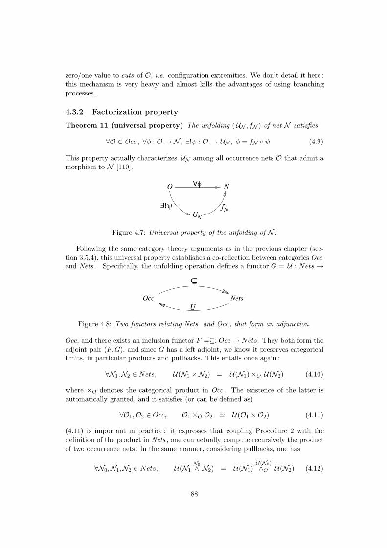
zero/one value to cuts of O, i.e. configuration extremities. We don’t detail it here :this mechanism is very heavy and almost kills the advantages of using branchingprocesses.
4.3.2 Factorization property
Theorem 11 (universal property) The unfolding (UN , fN ) of net N satisfies
∀O ∈ Occ , ∀φ : O → N , ∃!ψ : O → UN , φ = fN ◦ ψ (4.9)
This property actually characterizes UN among all occurrence nets O that admit amorphism to N [110].
A
%
E
!&UN
fN
O N
Figure 4.7: Universal property of the unfolding of N .
Following the same category theory arguments as in the previous chapter (sec-tion 3.5.4), this universal property establishes a co-reflection between categories Occand Nets . Specifically, the unfolding operation defines a functor G = U : Nets →
U
NetsOccU
Figure 4.8: Two functors relating Nets and Occ , that form an adjunction.
Occ, and there exists an inclusion functor F =⊆: Occ → Nets. They both form theadjoint pair (F,G), and since G has a left adjoint, we know it preserves categoricallimits, in particular products and pullbacks. This entails once again :
∀N1,N2 ∈ Nets, U(N1 ×N2) = U(N1)×O U(N2) (4.10)
where ×O denotes the categorical product in Occ . The existence of the latter isautomatically granted, and it satisfies (or can be defined as)
∀O1,O2 ∈ Occ, O1 ×O O2 < U(O1 ×O2) (4.11)
(4.11) is important in practice : it expresses that coupling Procedure 2 with thedefinition of the product in Nets , one can actually compute recursively the productof two occurrence nets. In the same manner, considering pullbacks, one has
∀N0,N1,N2 ∈ Nets, U(N1N0∧ N2) = U(N1)
U(N0)∧O U(N2) (4.12)
88

where the pullback ∧O in Occ is defined by
∀O0,O1,O2 ∈ Occ, O1O0∧O O2 < U(O1
O0∧ O2) (4.13)
and so ∧O can again be computed recursively.
As we have seen in chapter 3, the factorization property of a structure encodingruns of a compound system is the first ingredient towards distributed diagnosisalgorithms. So we are already in very good shape. The next ingredient is an adequatenotion of projection, that we examine in the remainder of this chapter.
t 1 t 2
t 5
c
a
t’5
t 3 t 4
d
b
! !
Figure 4.9: The net in Fig. 4.6, expressed as a product of two components.
But before, let us illustrate the interest of a relation like (4.10). The net N inFig. 4.6, left, can be decomposed as the product of two smaller nets N = N1×N2, seeFig. 4.9. Eq. (4.10) expresses that UN is thus the product, in the sense of occurrencenets, of the UNi depicted in Fig. 4.10. The latter are simple trees, since the Ni areautomata. One first notices that unfoldings grow in width as one progresses in“length” (the time dimension). This is precisely one of the drawbacks addressed bythe next chapter. Now, considering the number of possibilities to fire t5 (resp. t′5) inUN1 (resp. UN2), one finds two solutions for the first occurrence of t5, then four forthe second occurrence, etc. In the expanded product UN , they result in 2× 2 = 4possibilities to fire the first occurrence of (t5, t′5) (see Fig. 4.6, right), then 16 = 4×4for the second occurrence, etc. In other words, the factorized form of UN is morecompact than the expanded one, just like (a + b + c + ...)p is more compact thanits expanded form. Therefore it is likely that processings based on the factorizedform of UN will be more efficient than processings on the expanded form, as it wasalready the case in chapter 3 with sequential semantics.
4.4 Distributed diagnosis : the unfolding approach
As soon as the product is defined in Occ , a natural notion of projection becomesavailable. We first explore how far one can go with this notion, in terms of modularcomputations for the diagnosis problem.
Notations : notice that we denote by Ob the observations, and by O general oc-currence nets or branching processes.
89

t 5
t 1
c
a
t5
t 2
t 5 t 5
t 1 t 2
t 5 t 5
t 1 t 2
c
a
c c
a
c c
a a a
a
t’5t’5 t’5t’5
t 3 t 4 t 3 t 4
t’5
t 3
d
b
t’5
t 4
d
b
d d
b b
d d
b b
b
. . . . . .
Figure 4.10: Unfoldings of the two components of Fig. 4.9.
4.4.1 Projection
Natural projection. Let us first consider two nets N1,N2, and branching pro-cesses (Oi, fi) of these nets. The occurrence net O = O1 ×O O2 is associatedto two morphisms ψi : O → Oi. Combined to the foldings fi, they yield thefi ◦ ψi : O → Ni, and since one has morphisms from O to the Ni, by the uni-versal property of N = N1 ×N2 (prop. 9), there exists a unique f : O → N suchthat fi ◦ ψi = f ◦ φi, where φi : N → Ni. It is easily checked that f is a folding,which makes O1 ×O O2 a branching process of N1 ×N2 (Fig. 4.11).
O1xoO2O= O2O1
N1 N2N= x N2N1
f2f1
&1
&2
%2
%1
f
Figure 4.11: The product of two branching processes yields a branching process ofthe product.
We take as projections of O the two occurrence nets O′i = ψi(O). They are
prefixes of the original factors Oi (O′i ; Oi) and satisfy O = O′
1×O O′2. Referring to
notions introduced in the previous chapter (end of section 3.1.2), the O′i thus form
the minimal product covering of O, in the sense that taking a strictly smaller prefixO′′
i # O′i of one factor kills the equality.
This is illustrated by the example in Fig. 4.12, that depicts the product of twoconfigurations (κ1, left and κ2, right). The product lies in the middle, and all labels{α,β} are supposed shared. Observe that the event t3 of κ1, labeled by β, finds nopartner in κ2 and thus vanishes. So ψ1(κ1 ×O κ2) reduces to events t1 and t2. Thisexample also illustrates that the product of two configuration is not necessarily a
90

configuration : there may exist different associations of their events. Finally, noticethat the two concurrent events t1, t2 of κ1 inherit a causality relation of κ2 in theproduct, either in one direction or the other.
! !
!!
t1!
a
b
t2!
c
d
t3"
e
t4t1 t4
t2 t5t5 t1
t2
f
g
h
g’
h’
a
b
c
d
d’ b’
t5
t4
f
g
h
!
!
Figure 4.12: Product (center) of two configurations (left and right), that share allevent labels, i.e. α and β.
To define the projection of any branching process ofN = N1×N2, we consider thesame scheme with UN instead of O. From UN = UN1 ×O UN2 stated in (4.10), andits associated morphisms ψi : UN → UNi , one can define the projections O′
i = ψi(O)for any branching process O ⊆ UN of N . One has O′
i ⊆ UNi which obviously makesthem branching processes of the Ni. They form the minimal product covering ofO in the sense that O ; O′
1 ×O O′2, and replacing one of the factors O′
i by a strictprefix O′′
i # O′i kills this prefix inclusion of O. So the projection keeps events of the
UNi that are strictly useful to O, and only them. Observe that O is included in itsproduct covering (whence the name), and is equal to it iff O was already in productform.
Projection operator. We now move to the general case N = N1× . . .×NN andconsider O = O1×O . . .×O ON where each Oi is a BP of Ni. For I ⊆ {1, . . . ,N}, westill use notations NI = ×i∈INi and OI = ×O
i∈IOi. By associativity of ×O, we canwrite O = OI ×O OIc and define ΠI(O) as ψI(O). This projection operation gener-alizes to any OJ , for J ⊆ {1, . . . ,N}, by ΠI(OJ ) ! ΠI∩J(OJ). And by associativityof ×O, one easily checks that
∀I, J ⊆ {1, . . . ,N}, ΠI ◦ΠJ = ΠI∩J (4.14)
which corresponds to axiom (a1).In practice, it is quite easy to compute the projection of a BP : to get ΠI(OJ ),
it suffices to remove conditions and events not labeled by NI , and to “trim” theresult, i.e. to recursively merge isomorphic events in order to satisfy the parsimonycriterion (requirement 2 in the definition of a BP).
Minimal product covering. This notion applies as above :
∀O ; UN , O ; O′1 ×O . . .×O O′
N where O′i = Πi(O) ; UNi (4.15)
∀O′′i ; UNi , ∃j : O′′
j # O′j ⇒ O '; O′′
1 ×O . . . ×O O′′N (4.16)
91

In (4.15), one has equality iff O admits a product form : O = O1×O . . .×O ON , andin that case O′
i ; Oi. Moreover, one has O′I = ΠI(O) = ×O
i∈IO′i with O′
i = Πi(O).
4.4.2 Centralized diagnosis
Single sensor. The setting is like in the previous chapter : net N produces ahidden run κ, that is only observed through the labels of Λ′ ⊆ Λ that it produces.But what does it mean to observe the partial order of labels λ(κ)|Λ′ ?
Things become clear when one assumes that labels are logged in sequence bya sensor. So instead of λ(κ)|Λ′ one actually sees a linear extension of this partialorder, under the assumption that the observation process is not anti-causal : visibleevents that are causally related can’t lead to labels observed in the reversed order.However, two concurrent events could produce labels observed in any order.
Now, the observed labels may not all be ordered : indeed, when two visible labelsare collected on different sensors, the possible causal link relating these events isgenerally lost, unless some specific mechanism is deployed to preserve it. Therefore,as a general situation we assume that our observation Ob is a weakened version ofan extension of λ(κ)|Λ′ (see Fig. 4.13 for an example).
!
" )
!
" )
!
" )
t1
t2 t4
t3
d
e
fc
a
b)"
#! o1 o2
o3
!"
)
Figure 4.13: A hidden configuration κ (left), and an observed partial order of itslabels, expressed as a configuration (right). γ is supposed to be invisible, i.e. Λ′ ={α,β, δ}. The second plot is the partial order on visible labels induced by κ. Theordering of α and δ (third plot) may be created by the sensor that collects them. Bycontrast, the causality relation α → β may be lost if these labels are collected bydifferent sensors (fourth plot).
As a partial order of labels, Ob can be encoded under the form of a configuration(a LMCON), and a run κ of N is a valid explanation of Ob if it perfectly synchronizeswith Ob, i.e. if ψb
O(κ×O Ob) = Ob. To compute them all at once, consider
D = UN ×O Ob (4.17)
Not all maximal configurations of D explain entirely Ob, they may explain only aprefix of Ob and then be blocked. But those that do explain all Ob form a configura-tion set closed by concurrent extension (see lemma 8). In other words, it suffices tocut off dead branches of D, then take the remaining maximal configurations to getall solutions to the diagnosis problem, once projected back on UN . For simplicity,we assume in the sequel that the diagnosis is given by (4.17) above.
92

Multiple sensors. We now assume that N sensors are collecting labels producedby transitions of net N , and possibly observe the same labels. For example sensor ireacts to labels of Λ′
i and produces configuration Obi as observation. Specifically, Ob
iis a weakened version of some extension of λ(κ), restricted to Λ′
i. It is important tonotice that the same extension of λ(κ) lies behind all the Ob
i , otherwise the sensorscould observe in different orders two concurrent events, which would lead to aninconsistency. We easily get back to the previous case by defining
Ob = Ob1 ×O . . .×O Ob
N (4.18)
as our joint observation.
! "1* ={ , }’O1a b c d
" !!
O2a’ b’ c’ d’ e’
# # " #
" #* ={ , }2’
a b c d!!
a’ b’ e’c’ d’
"
## #
O1 O2x O
Figure 4.14: Two observed configurations, on sensors sharing label β, and the re-sulting equivalent joint observation.
This deserves several comments. First, observe that the Obi synchronize on the
labels they jointly observe. If the Λ′i are disjoint, putting all observations together
simply amounts to juxtaposing the Obi , which is much simpler than the complex
computation of all interleavings of Fig. 3.18. Translated in the true concurrencysemantics, the latter becomes Fig. 4.14. Secondly, taking as observation the productof the Ob
i may yield a general occurrence net, not necessarily a configuration (seeFig. 4.12). This doesn’t change much the theory : it suffices to take as solution tothe diagnosis problem a maximal configuration of D that projects into a maximalconfiguration of Ob, equivalently into maximal configurations of the Ob
i (i.e. the Obi
themselves).
4.4.3 Distributed diagnosis
Algebraically, the situation is pretty much the same as for sequential semantics (sec-tion 3.6.3). We now assume that the supervised system N is obtained by assemblingsmaller nets Ni, that we call sites : N = N1 × . . .×NN . Each of the Ni is attachedto a specific sensor collecting labels of Λ′
i ⊆ Λi and producing observation Obi , as
above. By injecting (4.10) and (4.18) into (4.17), one gets
D = [UN1 ×O Ob1]×O . . .×O [UNN ×O Ob
N ] (4.19)
93

This relation expresses that the global diagnosis corresponds to the synchronizationof local diagnoses Di = UNi×OOb
i computed for each site. Our objective is to derivethe minimal product covering of D, that is the branching processes Oi = ΠNi(D), orequivalently the D′
i = ΠNi×Obi(D) = Oi ×O Ob
i . They correspond to coherent localviews of D, in the sense that they satisfy
D = [O1 ×O Ob1]×O . . .×O [ON ×O Ob
N ]= D′
1 ×O . . . ×O D′N (4.20)
Of course, a crucial point is to derive the Oi or the D′i without computing D itself,
since the latter can be a huge object (recall that products generally multiply tran-sitions). So we aim at deploying the modular computation formalism of chapter 2.
Translation into pullbacks. As in the case of sequential semantics (section 3.6.3),we don’t yet have a clean theory that would allow to project a branching processon a label set, and would allow as well to combine the resulting object (probablyan event structures carrying labels) with another branching process5. By contrast,there exists a natural notion of projection on sites, which suggests to use pullbacksto transmit information from component to component, see (3.44).
We thus restate N as N = S1 ∧ . . . ∧ SM where components Sj are defined bySj = NIj = ×i∈IjNi and cover all the sites : ∪jIj = {1, . . . ,N}. One has
UN = US1 ∧O . . . ∧O USM (4.21)
and similarly
D = [US1 ×O ObI1 ] ∧O . . . ∧O [USM ×O Ob
IM]
= D1 ∧O . . . ∧O DM (4.22)
where each local diagnosis Dj incorporates by ObIj
observations on all sites Ni ofcomponent Sj. It is not necessary to duplicate observations Ob
i when site Ni appearsin several components. It suffices to “distribute” the Ob
i on components, in such away that each Ob
i appears at least once in (4.22). But taking all observations ObIj
on Sj has the advantage of “ maximally reducing” USj , an interesting property formodular computations.
The distributed diagnosis problem now amounts to computing the OIj = ΠIj (D),or equivalently the D′
j = ΠSj×OObIj
(D) = OIj×OObIj
, that form the minimal pullback
covering of D :
D = [OI1 ×O ObI1 ] ∧O . . . ∧O [OIM ×O Ob
IM]
= D′1 ∧O . . . ∧O D′
M (4.23)
If necessary, the ΠNi(D) of the minimal product covering can be deduced from thelarger D′
j .
5This can probably be done, but remains a research topic.
94

Misleading projections. This notion underlines a problem that arises with nat-ural projections defined on branching processes. Computing projection O′
I = ΠI(O)amounts, in part, to selecting some events and conditions in O. But this operationmay forget causalities or conflicts that were linking them (see. Fig. 4.15). As a re-sult, two events or conditions may unduly appear as concurrent after projection, andthus be allowed to appear in the same configuration, or with a reversed causality,whereas this would have been impossible in the original branching process O.
t 1 t 2
a
b d
c
t1 t2
a
b d
ce
gf
t1
t 2
a
b
c
d
e
f
g
Figure 4.15: Two branching processes (left and right) that create a fake concurrency(center) once the influence of the central variable is discarded by the projection. TheBP on the left loses a conflict relation, the one on the right loses a causality relation.
We say that O′I = ΠI(O) is not misleading iff every configuration κ′ in O′
I canbe obtained as the projection of a configuration κ of O. One has :
Lemma 9 Let us say that Ni is a simple site if, as a LMC net, it is composed ofa single state variable. Projections of branching processes on simple sites are nevermisleading.
This is due to the fact that a BP of a simple site can’t have concurrent events. Thenext section is precisely devoted to defining a notion of projection that keeps trackof useful conflicts and causalities.
Separation theorem. We are now well equipped to state the separation theorem,that forms the backbone of modular computations.
Theorem 12 Let I,K ⊆ {1, . . . ,N}, and take J = I ∩K. Let OI ,OK be branch-ing processes of NI ,NK respectively, and assume that shared sites NJ capture allinteraction labels between NI and NK , i.e. ΛI ∩ΛK ⊆ ΛJ . If projections ΠJ are notmisleading, then
ΠJ(OI ∧O OK) = ΠJ(OI) ∧O ΠJ(OK) (4.24)
This weak form of axiom (a3) reproduces the formal setting of section 3.6.3, so wecan still derive propagation and merge primitives :
95

Proposition 11 Let I, J,K ⊆ {1, . . . ,N}, and let OI ,OJ ,OK be branching pro-cesses of NI ,NJ ,NK respectively. If ΛI ∩ ΛK ⊆ ΛJ , denoted I|J |K, and if projec-tions ΠJ are not misleading, then
ΠJ(OI ∧O OJ ∧O OK) = ΠJ(OI ∧O OJ) ∧O ΠJ(OJ ∧O OK) (4.25)ΠI(OI ∧O OJ ∧O OK) = ΠI [OI ∧O ΠJ(OJ ∧O OK)] (4.26)
Compared to the chapter on sequential semantics, the essential change is thus thenew ingredient of “non misleading” projections. To show the importance of thisassumption, let us examine the counter-example of Fig. 4.16. The two BPs O1 (left)and O2 (right) have the same projection on variables a and c (center), which allowsto fire t1 and t2 concurrently. However, in reality O1 imposes to fire t1 before t2,while O2 imposes the converse, so their pullback O1 ∧O O2 contains no event at alland reduces to the initial conditions {a, e, c, h}.
t 1
t 2
a
b
c
d
e
f
g
t1
t 2
a c
b
di
j
h
t1
a
b
t2
d
c
Figure 4.16: With misleading projections, theorem 12 doesn’t hold.
Support graph for modular computations. Identical to section 3.6.3.
4.4.4 Example
O1 O2S1 S2dg
c e fb
a
c
g
t1 t4 t5 t6t2 t4t3 t1
#
#
!!"
"
!# ) #
)
bb
Figure 4.17: Two components S1 = N1 ×N3 and S2 = N3 ×N2 formed of two siteseach, and observations Ob
1,Ob2 on these components.
96

The center of Fig. 4.17 represents two components S1 = N1 ×N3,S2 = N3×N2
that share site N3, in charge of flipping tokens from g to c. Their pullback amountsto superimposing this common sub-net. With a slight abuse of notations, we assumethe pullback is performed taking transition names as labels. Transitions of these netsproduce labels (Greek letters) that have been collected under the form of the twosequences Ob
1 and Ob2. On this example, we assume that the labels used for the
pullback differ from those collected by sensors, so nets are provided with two labelsets (or equivalently with a synchronization algebra [111]), which doesn’t changemuch the theory but introduces some flexibility.
g
g
c
g
cd
eg
g e
f
dc
c d
fa
b
a
a
b
g
c
b b b
g
b c
t4
t1
t4
t1
t6
t5
t4 t6
t5t1
t1
# #
#
. . .
#
)
)t1t2t2
t1
t4
t1
t3 t3
t2*
*
*
. . .
! ! ! !
" "
! !
c
Figure 4.18: Local diagnoses Di = USi ×O Obi (left and right), and the message
Π3(D1) from S1 to S2 (center).
The local diagnoses D1,D2 are depicted in Fig. 4.18. They are obtained byunfolding each Si and taking the product with the corresponding Ob
i . Events andconditions in gray are discarded by the product. Observe that in D2 the first firingof t6 is discarded although it matches the first observation γ. The reason is that t6has no future, and so can’t lead to an explanation for the next observation δ. Thiscorresponds to a dead branch in US2 ×O O2. The BP in the middle represents theprojection of D1 on the interface net N3, which is the message from S1 to S2. Itessentially expresses that observations Ob
1 do not allow a second firing of t1. The starsnext to conditions indicate possible stop points6, i.e. projections of configurationsthat explain all observations Ob
1. Once inserted into D2, by a pullback operation,this message removes some of the explanations : a single configuration remains inD′
2 (Fig. 4.19).6As previously mentioned, the notion of stop point for BP is a 0/1 function on cuts of this BP.
97

g
g
c
g
c
a
b
a
a
b
g
c
g
d
g e
f
d
g
c
e
t4
t1t1
t4t3 t3
t2
t4
t5
t6
t1
t4
t1
" "
! !
#
#
)
#
*
*
*
Figure 4.19: Insertion of the message Π3(D1) into D2 by D′2 = Π3(D1) ∧O D2.
The message in the reverse direction (Fig. 4.20) is longer and also differs by theposition of stop points : D2 can’t stop before the first t4 is fired. Once insertedinto D1, this message renders impossible the solution (t2, t3) because this privatetrajectory doesn’t provide the sequence (t1, t2) to S2. So again a single configurationremains possible in D′
1.
g
g
c
g
c
g
cd
eg
g e
f
c d
a
a
b
g
c
ga
b
t4
t1
t4
t1
*
*
*
t4
t1 t5
t4 t6
t1
# #
#
)
t1
t4t3t3
t2
"
!!
"
Figure 4.20: Message from S2 to S1, and its insertion into D1 by D′1 = Π3(D2)∧OD1.
Notice that putting together the reduced local diagnoses yields a unique solutionto the problem : D = D′
1 ∧O D′2 contains a single maximal configuration (Fig. 4.21).
The latter reveals that α necessarily appeared before the first γ in Ob2, while β
is concurrent with Ob2. Moreover, the observed sequences do correspond to true
98

causalities in the underlying system. So we have rediscovered the causality relationsof our observations.
a g
cd
d
g ea
b
f
t1
t3 t4
t5
t6
"
!
#
)
#
Figure 4.21: Global solution to the diagnosis problem.
Of course, this example doesn’t manifest the interest of modular computations :the factorized form US1 ∧O US2 has the same complexity as the expanded form US .The advantage appears when the two systems have different ways of producing andconsuming the resources of their interface N3.
4.4.5 Involutivity
MC branching processes are involutive, i.e. satisfy O ∧O ΠI(O) = O. So we are inthe setting where message passing algorithms converge on any graph, and producean approximation of the reduced local diagnoses. Instead of the D′
j = ΠSj×OObIj
(D),
one gets the upper approximations D′′j that satisfy
∀i,D′j ; D′′
j ; Dj and D = D′′1 ∧O . . . ∧O D′′
M (4.27)
It can also be shown that MPA perform a progressive reduction (theorem 4), andthat the limit D′′
M satisfies the local extendibility property (theorem 3).
Misleading projections. What happens if the presence of misleading projectionsis ignored ? Theorem 12 is not completely lost : instead of (4.24), one gets
ΠJ(OI ∧O OK) ; ΠJ(OI) ∧O ΠJ(OK) (4.28)
which means that message passing algorithms do propagate constraints, but not all ofthem. This is due to the fact that misleading projections create fake concurrencies,and thus fake configurations. MPA still converge on trees in a finite number of(useful) steps. In reason of involutivity, convergence is also granted on any graph.And in both cases the limit D′′
j satisfies (4.27).
99
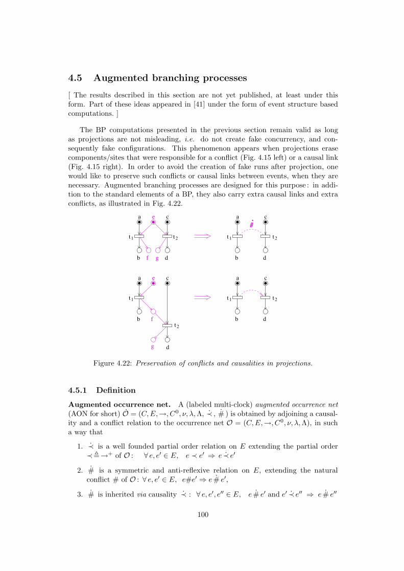
4.5 Augmented branching processes
[ The results described in this section are not yet published, at least under thisform. Part of these ideas appeared in [41] under the form of event structure basedcomputations. ]
The BP computations presented in the previous section remain valid as longas projections are not misleading, i.e. do not create fake concurrency, and con-sequently fake configurations. This phenomenon appears when projections erasecomponents/sites that were responsible for a conflict (Fig. 4.15 left) or a causal link(Fig. 4.15 right). In order to avoid the creation of fake runs after projection, onewould like to preserve such conflicts or causal links between events, when they arenecessary. Augmented branching processes are designed for this purpose : in addi-tion to the standard elements of a BP, they also carry extra causal links and extraconflicts, as illustrated in Fig. 4.22.
t 1 t 2
a
b d
ce
gf
t1 t 2
a
b d
c
t1 t2
a
b d
c
t1
t2
a
b
c
d
e
f
g
#.
Figure 4.22: Preservation of conflicts and causalities in projections.
4.5.1 Definition
Augmented occurrence net. A (labeled multi-clock) augmented occurrence net(AON for short) O = (C,E,→, C0, ν,λ, Λ, ≺ , # ) is obtained by adjoining a causal-ity and a conflict relation to the occurrence net O = (C,E,→, C0, ν,λ, Λ), in sucha way that
1. ≺ is a well founded partial order relation on E extending the partial order≺!→+ of O : ∀ e, e′ ∈ E, e ≺ e′ ⇒ e ≺ e′
2. # is a symmetric and anti-reflexive relation on E, extending the naturalconflict # of O : ∀ e, e′ ∈ E, e#e′ ⇒ e # e′,
3. # is inherited via causality ≺ : ∀ e, e′, e′′ ∈ E, e # e′ and e′ ≺ e′′ ⇒ e # e′′
100

The augmentation of O with ≺ and # amounts to replacing some concurrency linksbetween events either by a causality or by a conflict. We call # \ # (resp. ≺ \ ≺)the extra conflict (resp. causality) relations. Notice that (E, ≺ , # ) is a regularevent structure, therefore the objects we have introduced are a mixture betweenevent structures and occurrence nets. The importance of preserving conditions willappear in the definition of projections.
Relations ≺ and # are defined on E but naturally propagate to all nodes ofO, by transitivity for ≺ and by inheritance for # . As for standard occurrencenets, events e1 and e2 are said to be concurrent, denoted by e1⊥⊥e2, iff ¬(e1 ≺ e2),¬(e2 ≺ e1) and ¬(e1 # e2). Co-sets and cuts are defined from ⊥⊥ in the usual way.
Prefix. The notion of prefix differs slightly from the one defined for standardoccurrence nets. The AON O′ = (C ′, E′,→, C0, ν,λ, Λ, ≺ , # ′) is a prefix of O, stilldenoted by O′ ; O, iff
• C ′ and E′ are left causally closed in O for ≺ , and ∀e ∈ E, [e ∈ E′ ⇒ e• ∈ C ′],
• # ′ contains the restriction of # to E′.
It is therefore sufficient to reinforce the conflict relation # of O to obtain a strictprefix of O, provided this reinforcement yields a valid augmented occurrence net.Intuitively, taking a prefix means reducing the set of possible configurations, whichthis definition expresses (see also below).
Configuration. An augmented configuration κ of O (or configuration for short)is a conflict-free prefix of O, for # . The augmented configuration κ is thus also aconfiguration of O enriched with extra causality relations on its events. Obviously,the converse doesn’t hold : a configuration of O, may not be transformable intoa configuration of O, even if causality relations are added, because # is strongerthan #.
Morphism. A morphism φ : O1 → O2 of augmented occurrence nets is a MC netmorphism φ : O1 → O2 that partially maps relations ≺1 and #1 to ≺2 and #2
∀ e1, e′1 ∈ E1, φ(e1) ≺2 φ(e′1) ⇒ e1 ≺1 e′1
and φ(e1) #2 φ(e′1) ⇒ e1 #1 e′1
Notice that causality and conflict relations due to → are preserved, only extra rela-tions of ≺1 \ ≺1 and #1 \ #1 can be erased and transformed into concurrency. Somorphisms still preserve runs, i.e. configurations.
Augmented branching process. The pair (O, f) is an augmented branchingprocess (ABP) of net N iff
1. f : O → N is a folding of O into N ,
2. if κ and κ′ are isomorphic (augmented) configurations of O, with identicalfolding into N , then κ = κ′.
101

The second requirement generalizes the parsimony criterion appearing in the defi-nition of an ordinary BP, and constrains an ABP to represent at most once a given“augmented” run of N . Notice that the parsimony criterion of ordinary BP doesn’thold here : a given co-set X of O may be followed by two distinct events e, e′ mappedto the same transition of N by f . This happens when e and e′ are not related to theother events of O in the same manner for ≺ , which means that these events havedifferent pasts. This is illustrated in Fig. 4.23. As a consequence, the pair (O, f)obtained by removing the extra relations, generally violates the parsimony criterionof ordinary BP.
a
c’ c’
c
c" c"b’ b’
a’b
a b
a’ b’b’
t3t1
t2 t2
t1 t2 t2
Figure 4.23: Projection of a BP that removes component c (and thus t3). This yieldstwo runs : one where t1 precedes t2, and one where t1 and t2 fire concurrently.
In the sequel, we will make use of generalized ABP (GABP) of a net N , whichmeans that point 2 of the definition may not be satisfied. Obviously, when this isnot the case, there exists a simple recursive trimming procedure that makes O atrue ABP of N . We will denote by Trim(O) this operation.
4.5.2 Key property
Augmented branching processes enjoy several interesting properties. For example,removing the extra conflicts in O, i.e. replacing # by #, yields another ABP of N ,that we call the structure of O. One easily proves that structures have finite width,at any height, which allows us to prove results on ABP by recursion on the height.
a
a’
a"
b
b’
a b
a’
b"
b’
a b
b’a’
t1
t3
t2
t4
t2t1 t1 t2
U =##
. .
.
Figure 4.24: Intersection of two ABP (inherited conflicts are not represented, forclarity).
Several important properties are related to the ability of ABP to describe sets ofruns of N . If every configuration of O1 is isomorphic to a configuration of O2, then
102

O1 is isomorphic to a prefix of O2. In terms of operations on ABP, one can definethe intersection O1∩O2 that exactly contains augmented configurations appearingin both Oi. It is obtained as the intersection of the structures of the Oi, followed bya suitable definition of the extra conflicts (see Fig.4.24). In the same manner, onecan also define the union O1∪O2, that exactly contains configurations appearing atleast in one of the Oi (see Fig.4.25). This strongly contrasts with ordinary branchingprocesses, where the union introduces redundant runs.
a
a’
a"
b
b’
a b
a’
b"
b’
a
a’
a"
b
b’
b"
t1
t3
t2
t4
t2t1 t1
t3
t2
t4
.#
U =.#.
Figure 4.25: Union of ABP (only minimal conflicts are represented).
In reality, these properties are consequences of
Proposition 12 There is a one to one correspondence between prefix-closed sets of(augmented) configurations of N and augmented branching processes of N .
So ABP are stronger that ordinary BP in the sense that one is not limited to config-uration sets closed by concurrent suffix extension (compare to lemma 8). So unionsand intersections of ABPs can be understood as operating on configuration sets.
Proposition 12 deserves one extra comment. We know that distributed compu-tations are possible with configuration sets, just like in the sequential semantics onecan compute with sub-languages. As ABP provide a compact encoding of any con-figuration set (up to prefix closure, which is not a severe limitation), it is likely thatone can compute with them. The effort simply consists in proving that computationscan be directly performed on ABP, without transforming them into configurationsets.
Since we have the union of ABP, one could define a notion of “augmented un-folding,” by taking the union of all augmented configurations of N . This is of littleinterest, however. First of all because that would yield a huge object, containing allextensions of all (standard) configurations of N . Secondly, this object wouldn’t havethe universal property, for the definition of morphisms that we took. Consider forexample the ABP O in Fig. 4.23, right. The augmented configuration κ of N formedby a firing of t1 followed by a firing of t2 can be sent into O with two morphisms :one that preserves the causality, and one that erases it.
4.5.3 Operations on ABP : product, pullback, projection
Product. Let O1, O2 be two AON, we define their product O = O1 ×O O2 in thecategory ˙Occ of augmented occurrence nets by extending the recursive procedure
103

computing the product in Occ . This takes the following form, where the ψi : O → Oi
as canonical mappings
Procedure 3
• Initialization :
– C0 = C01 6 C0
2 , and the ψi : C0 → C0i follow accordingly,
– set C = C0 and E = ∅ (→, ≺ and # are empty as well).
• Recursion (until stability) :
– Let κ be a configuration of O and X an extremal co-set of κ,let κi = ψi(κ) and Xi = ψi(X), i = 1, 2
– if ∃(e1, e2) ∈ E1 × E2, λ1(e1) = λ2(e2), •ei = Xi,and ' ∃e ∈ E, •e = X, ψi(e) = ei,
∗ create such e in E,∗ create a set X ′ = X ′
1 6X ′2 of |e•1| + |e•2| new conditions in C,
with e• = X ′ and ψi(X ′i) = e•i ,
∗ ∀e′ ∈ κ ∩ E, set e′ ≺ e if ψi(e′) ≺i ψi(e) for some i,∗ ∀e′ ∈ E, set e′ # e if ψi(e′) #i ψi(e) for some i.
– if ∃e1 ∈ E1, λ1(e1) ∈ Λ1 \ Λ2, •e1 = X1
and ' ∃e ∈ E, •e = X, ψ1(e) = e1
∗ create such e in E,∗ create a set X ′ of |e•1| new conditions in C,
with e• = X ′ and ψi(X ′) = e•1,∗ ∀e′ ∈ κ ∩ E, set e′ ≺ e if ψi(e′) ≺i ψi(e) for some i,∗ ∀e′ ∈ E, set e′ # e if ψi(e′) #i ψi(e) for some i.
– symmetrically for private events of O2.
Of course, Λ = Λ1 ∪ Λ2 and the labeling of events is inherited through the ψi, aswell as the partitioning ν on conditions. Observe that the recursion does not createall extra causalities and extra conflicts, but only the minimal ones. Therefore, inchecking configurations κ for possible extension, one must take into account thecausal closure and inheritance of conflicts.
This procedure resembles very much what one would obtain for the product inOcc , by coupling the unfolding procedure 2 to the definition of the product in Nets .Apart the treatment of ≺ and # , the difference is that events are connected to apair co-set plus configuration instead of a co-set only. This translates the differenceof the parsimony criteria of BP compared to ABP.
Proposition 13 Procedure 3 computes the categorical product in ˙Occ.
This entails the associativity of ×O. Proposition 13 has to be proved directly since×O can’t be derived from the product in Nets via a suitable adjunction, this time.
104

Notice that the product of AON is very close to a product of (labeled) event struc-tures [17, 26, 106, 111], which is consistent with their nature.
Considering augmented branching processes, the picture is not as nice as withordinary BP, because the parsimony criterion is lost by the product. One has
Proposition 14 Let (O1, f1), (O2, f2) be ABP of N1,N2 respectively. Then O =O1 ×O O2 provided with the folding f = (f1 ◦ ψ1, f2 ◦ ψ2) is a generalized ABP ofN = N1 ×N2. A true ABP of N is obtained by trimming O.
This phenomenon is illustrated in Fig. 4.26. Fortunately, however, computing withgeneralized ABP is not so much bothering, except for the size of the objects involved :
Lemma 10 Let O1, . . . , ON be GABP of N1, . . . ,NN resp., then
Trim(O1 ×O . . . ×O ON ) = Trim[Trim(O1)×O . . .×O Trim(ON )] (4.29)
For distributed computations on ABP, one can very well include a trimming in thedefinition of the product. This loses the canonical morphisms from the productto its factors, but doesn’t change the results in terms of configuration sets of theunderlying nets.
a b
a’ b’ b’
a c
c’b
b’
a’
c" b’ c"
a c
c’b
a’
b’ c"
c
c’
c"
t1 t2 t2! " " t3t1
t2t4 t2t4" "
! t3t1
t2t4
!
"
t3
t4
!
"
=xo
Figure 4.26: From left to right, two ABP O1, O2, their product O1 ×O O2, andTrim(O1 ×O O2).
Pullback. Moving to pullbacks, it is not known whether they all exist in ˙Occ. Butin the simple case where morphisms φi : Oi → O0 are partial functions, the pullback
O1O0∧O O2 can be obtained with a slight modifications of Procedure 3 above. And it
enjoys the same properties as the product. This is the only important case for ourcomputations.
As a remark in passing, notice that the pullback behaves differently on ABPthan on BP. For example, if O,O′ are two ordinary BP of the same net, thenO ∧O O′ coincides with O ∩ O′. This is not true anymore with ABP : one hasO ∩ O′ ; Trim(O ∧O O′).
Minimal product covering. This property doesn’t change. Given O = O1 ×O
. . . ×O ON , and O′i = ψi(O), one still has O′
i ; Oi, O = O′1 ×O . . . ×O O′
N and theminimality of the O′
i. Same thing for the pullback.
105

Projection. For product ABP O as above (or their prefixes), taking the imageψi(O) erases causality and conflict relations inherited from the other Oj . This wasprecisely the weakness of computations based on ordinary BP. Therefore we ratherdefine the projection as follows :
Πi(O) = Trim[ O|Dom(ψi) ] (4.30)
The restriction preserves all inherited causality/conflict relations, while selectingonly conditions and events that correspond to component Ni. The relation O =Π1(O)×O . . .×O ΠN (O) is preserved.
Moreover, for an ordinary BP O = O1×O . . .×OON , one easily recovers minimalfactors O′
i = Πi(O) by removing all extra relations in Πi(O) and trimming the result.Therefore, one can take as intermediary objective the computation of the minimalproduct covering in terms of ABP.
4.5.4 Separation theorem
At this point, we have projections ΠI defined on ABP, that obviously satisfy ax-ioms (a1) and (a2), and a combination by pullback ∧ that satisfies axiom (a4) withthe empty ABP as neutral element. Only the central axiom (a3) is missing to enabledistributed computations.
Theorem 13 Let I,K ⊆ {1, . . . ,N}, and take J = I ∩K. Let OI , OK be branch-ing processes of NI ,NK respectively, and assume that shared sites NJ capture allinteraction labels between NI and NK , i.e. ΛI ∩ ΛK ⊆ ΛJ . Then
ΠJ(OI ∧O OK) = Trim[ ΠJ (OI) ∧O ΠJ(OK) ] (4.31)
This relation resembles more axiom (a3) if the trimming is introduced into ∧O toform ∧O. (4.31) becomes ΠJ(OI ∧OOK) = ΠJ(OI)∧OΠJ(OK). Notice that whenthe separation criterion is violates, one still has ΠJ(OI ∧OOK) ; ΠJ(OI)∧OΠJ (OK).
With theorem 13, we are thus fully equipped to perform the distributed computa-tions of the previous section, without the assumption of non-misleading projections.
4.5.5 Weak involutivity
As mentioned section 4.4.5 (see also sections 3.6.3 and 2.2.4), when a system N =S1 ∧ . . .∧SM doesn’t live on a tree, message passing algorithms (MPA) still providegood approximations of the reduced local diagnoses, provided computations areperformed on involutive objects. This is the case of branching processes :
OI ∧ΠJ(OI) = OI (4.32)
which corresponds to axiom (a8) section 2.2.4, so all MPA have a unique and identicalstationary point. The latter is formed of partially reduced local diagnoses, that forma (non minimal) pullback covering of the global diagnosis.
106

What about computations based on augmented branching processes ? Unfortu-nately, involutivity is lost, only a weak form remains : For OI and ABP of NI , onehas
OI ∧ ΠJ(OI) @ OI (4.33)
So composing an ABP with part of itself generally introduces extra (reinforced)configurations. This doesn’t mean however that turbo procedures are excluded forABP. Let us define the relation " on GABP of a net N by
O1 " O2 ⇔ O1 ; O1 ∧ O2 (4.34)
Proposition 15 The pre-order " on GABPs of N , satisfies axioms (a5,a6,a7).
So we are almost in an involutive setting. Let us define the equivalence relation ≡on (G)ABP of N by :
O1 ≡ O2 ⇔ O1 " O2 " O1 (4.35)
Then the involutivity is recovered provided one replaces = by ≡, i.e. (4.33) becomesOI ∧ ΠJ(OI) ≡ OI . So turbo algorithms based on ABP converge to a uniquestationary point, defined in terms of equivalence classes of ≡ (see theorems 2 and 4).These stationary classes are identical for all algorithms, but the latter may howeverreach different ABP in these classes.
a
a’ b’
ba b
a’ b’b’ b’a’a’
ba
t1 t2t1 t2 t2 t2t1 t1
Figure 4.27: Three equivalent ABP of the same net.
To help intuition, Fig. 4.27 depicts equivalent ABP of the same net. In substance,two GABP O1, O2 are equivalent if configurations of O1 are obtained by reinforcingconfigurations of O2 with extra causal links, and vice-versa. Or equivalently if eachGABP can be folded into the other.
Proposition 16 Equivalence classes of GABP are stable by ∧, by trimming, byintersection and by union of GABP. So they admit a minimal element.
In Fig. 4.27, the minimal net is the central one : the configurations of the others areobtained by reinforcing configurations of this minimal GABP.
By axioms (a5,a6,a7), we know that the equivalence of GABP is preserved bypullback ∧ (which includes trimming), and by projection Π. But these operationsdon’t preserve the minimality. Nevertheless, if all computations are followed by aminimization step, then involutivity in the strict sense is recovered.
In conclusion, one can indeed run turbo algorithms on ABP, and get the sameproperties as before, up to the minimality of the result. Which is not so muchbothering since in the end extra conflict and causality relations are discarded to getthe partially reduced local diagnoses.
107

4.6 Summary
This chapter is the equivalent of the previous one for the true concurrency semantics.We have introduced a second way of composing automata, in order to shape theresult as a safe Petri net and reveal the concurrency of transitions. Runs of thesenetworks of automata were defined as partial orders of events, or configurations. Asfor the sequential semantics, sets of configurations can be used as such, or encodedinto a more compact data structure called a branching process. One can go furtherin terms of compactness and define the counterpart of trellis processes for the trueconcurrency semantics (this is examined in the next chapter).
Concerning the distributed diagnosis problem, computations based on branch-ing processes have the same algebra as in chapter 3 : since projections on labels areimpossible, one is again constrained to use projections on sites to transmit informa-tion between components, and to use pullbacks to combine information. The maindifference lies in the nature of projections : using a naive definition allows to recycleexactly the approach of chapter 3, but this doesn’t capture all cases. In particu-lar, this strategy fails when components share an interface that enables concurrentevents, which may lead to “misleading projections.” To capture the general case,we have introduced the notion of augmented branching process, that combines thedefinitions of BP and of event structures. Their properties give them the flexibilityof configuration sets, and allow us to recover a clean definition of projection. Up tothis little modification, the rest of the algebra can be recovered. A slight differenceappears in the involutivity property, that takes a weaker form, but still sufficientlystrong to prove the convergence of turbo algorithms on cyclic networks of automata.
The nature of augmented branching processes, that resemble very much eventstructures, suggests that one could imagine working directly with event structures(see [41] for a first solution). A crucial point would be to define projections ofthese objects on label sets, which would bring us back to the simple case of the“direct graph” setting (see the language approach in section 3.4), and would avoidthe burden of using pullbacks. This is still a research issue.
Related work
The unfolding technique was introduced in the early 80’s [86, 110, 111] as a conve-nient way to represent runs of concurrent systems, in the so-called true concurrencysemantics. The expression “true concurrency” refers to the fact that runs are rep-resented as partial orders of events, by contrast with other models of concurrencylike Mazurkiewicz traces [27]. A trace is an equivalence class of sequences of events,where the equivalence is defined by the permutation of consecutive independentevents.
Unfoldings were revisited in the 90’s as a convenient tool for verification pur-poses [31, 82]. To this end, a crucial step is the construction of a finite completeprefix of the unfolding, i.e. a finite prefix that is sufficient to check a given propertyon the system. The most frequent definition of completeness refers to prefixes thatcontain all possible markings of the underlying net. Mac Millan proposed the firstconstruction [83], based on the key notion of adequate order (to compare configu-
108

rations). It was later refined by Esparza et al. [33, 34, 35] with the introduction ofsmarter adequate orders. It can then be proved that a finite complete prefix is notlarger than the marking graph of the underlying net. These approaches were algo-rithmic : the prefix was the output of a procedure. Khomenko [64, 67] introduced theidea of a canonical prefix, based on the notion of cutting context that defines a prioriat which events one should cut the unfolding. He also proposed efficient unfoldingalgorithms, making use of SAT solvers to find co-sets and possible extensions [60, 66].Among various applications of unfoldings in model-checking, several contributionsconsider reachability analysis [32, 36, 82, 83] and deadlock detection [65, 85].
The unfolding technique has been applied to various kinds of concurrent systems.Not only safe nets, but also semi-weighted nets [31], products of transition systems(as here) [35] or products of symmetrical nets [23]. More exotic concurrent modelshave also been explored. For example the important class of Petri nets with readarcs [7, 107], symbolic (or high-level) nets [19], networks of timed automata andtime Petri nets [16, 18], or graph grammars. Chatain, in particular, proposed animportant improvement with the idea of symbolic unfolding [19], see section 7.2.1.We jointly proved that symbolic unfoldings enjoy the same factorization properties asstandard unfoldings, which makes them natural candidates for distributed diagnosis.
Beside their intensive use in model-checking, partial order methods and unfold-ings have also been explored in the discrete event systems community, but apparentlywith a lower impact. Let us mention works in liveness enforcement [59], and severalinteresting contributions in controller synthesis [51, 52, 53]. In distributed diagnosisapplications, partial order methods have been used for state reconstruction in thecase of components interacting by places [14, 62, 63], with the interesting idea ofbackward unfolding. They have also been used, in parallel to our own work, forcommunicating automata [88]. The algebraization of distributed computations pre-sented in this chapter is original [9, 41]. The early versions of this approach havemuch benefited from the work of Winskel [109, 111, 112], and in particular [110],that enabled a clean and concise re-expression of all our results. Winskel introduceda simple and elegant way of deriving factorization results on unfoldings, by meansof category theory, that we use in different places of this document. So far, it seemsthat factorization aspects have not been exploited for modular model-checking ap-plications.
109

110

Chapter 5
Trellis unfolding for concurrentsystems
The trellis of an automaton represents all its possible runs in a compact structure,with a complexity that is typically linear in time (=length of runs). The idea is tomerge not only the common pasts, but also the common futures of two runs thatreach identical states at a the same time. Although such structures are familiarin communities dealing with Markov chains (control, digital communications, etc.),they are apparently new in the field of distributed processings, essentially becauseof the unnatural multi-clock ingredient that we had to introduce (chapter 4).
This chapter presents the generalization of this idea to true concurrency seman-tics, which has opened a new and promising research direction. Traditional unfold-ings can be seen as operating a double expansion of a concurrent system. Time, ofcourse, is unrolled (unfoldings are partial orders of events), but also conflicts areexpanded : each time there is a choice between n possible events, n branches arecreated, that will never meet each other again, since conflicts are inherited in an un-folding. By contrast, the notion of trellis is meant to unfold time, but not conflicts,and thus results in a more compact structure. Can such a simple idea be appliedto runs defined as partial orders ? Surprisingly, the answer is positive. And as anice feature, factorization properties can again be proved, provided merge points aredefined according to a vector clock, as in chapter 3. In reality, the algebraic simi-larities are extremely close, which allows us to replicate our approach to distributeddiagnosis, up to slight modifications of the key theorems.
The chapter is organized as follows. We first define trellis processes, and studytheir factorization properties. We then examine their relations to unfoldings. Fi-nally, we show that they admit a natural notion of projection, for which the sepa-ration theorem can again be established. This makes trellis processes suitable fordistributed diagnosis applications, which we illustrate on an example.
5.1 Trellis nets
This section defines the category of trellis nets, a family of nets where time is un-folded, but not necessarily conflicts. This category is thus intermediate between
111

Occ , occurrence nets, and Nets , safe Petri nets. We are still in the multi-clocksetting, that equips nets with a partition of places, used to identify components.
5.1.1 Definition
Pre-trellis net. The MC net T = (C,E,→, C0, ν) is a pre-trellis net iff it satisfies :
1. C0 = {c ∈ C : •c = ∅},
2. for every c ∈ C0, the automaton T|c has no circuit (i.e. its flow relation definesa partial order).
The definition of pre-trellis nets is much less restrictive than the definition of occur-rence nets. Specifically, point 1 is preserved, point 2 is weakened since →∗ is notany more required to define a partial order, and we have abandoned points 3 and 4 :conflicting branches are now allowed to merge on conditions.
e’2e 2
1e’ 1e"
1e
a
a
a
b
b
b
Figure 5.1: A pre-trellis net containing a circuit (thick arrows).
As an oriented graph, and by contrast with occurrence nets, a pre-trellis net isnot necessarily a partial order. Fig. 5.1 gives a counter-example of a pre-trellis netcontaining a circuit. However, one has the following property :
Lemma 11 No run of a pre-trellis net T can have a loop, i.e. can fill twice thesame place. As a consequence, the restriction T|σ of T to (nodes involved in) anyrun σ defines a partial order of nodes.
Therefore it makes sense to express runs of T as configurations κ rather than se-quences σ of transitions.
Configuration, trellis net. In an occurrence net, every event belongs at leastto one configuration, and so is reachable. This is not guaranteed anymore in apre-trellis net (see T1 in fig. 5.3), so we must refine our definition. We define aconfiguration κ of a pre-trellis net T = (C,E,→, C0, ν) as a sub-net of T satisfying
1. C0 ⊆ κ,
2. ∀e ∈ E∩κ, •e ⊆ κ and e• ⊆ κ : each event has all its causes and consequences,
3. ∀c ∈ C ∩ κ, |•c ∩ κ| = 1 or c ∈ C0 : each condition is either minimal or hasone of its possible causes,
112

4. ∀c ∈ C ∩ κ, |c• ∩ κ| ≤ 1 : each condition triggers at most one event,
5. the restriction of T to nodes of κ is a partial order.
1e’ 1e"
1ee 2 e’2
a
a
a
b
b
b
Figure 5.2: In the net of fig. 5.1, a subset of nodes satisfying the first four require-ments of a configuration, but failing on the last one.
This definition is close to the one introduced for ONs, apart from the fact that|•c| ≤ 1 is not automatic anymore in a pre-trellis net. So one must not only solveconflicts forward (point 4) but also backwards (point 3), to get a valid conflict-freeON. And the requirement that a configuration is “causally closed” is now spreadon 2, 3 and 4. The last point is suggested by lemma 11, and is indeed necessarysince points 1 to 4 alone do not guarantee this property (see a counter-example infig. 5.2). With the above definition, it is straightforward to check that a sequence σis a run of T iff it corresponds to a linear extension of some configuration κ of T .And so an event of a pre-trellis net is reachable iff it belongs to a configuration.
We thus define a trellis net (TN) as a pre-trellis net where each event belongsat least to one finite configuration (see fig. 5.3 for examples).
2e1e
e 3
a b
gf
c d
1e 3e
4e 4e
1e2e
3e
ba c
gd f
ba c
gd f
h i ihT 2T 1 T 3
Figure 5.3: T1 is a pre-trellis net but not a trellis net : event e4 is unreachable.The other nets are trellis nets : all events are reachable. In T2, e1 and e3 are notcausally related... but in conflict ! T3 displays a non binary conflict : {d, f}, {f, g}and {d, g} are all pairs of concurrent conditions, but the triple {d, f, g} appears inno run. Removing e2 in T3 doesn’t yield a valid prefix : we are back to T1 which isnot a trellis net.
Concurrency and conflict. From the definitions above, one sees that both ONsand TNs are graphical structures encoding families of configurations in different
113

ways. TNs offer the advantage of being more compact... at the expense of a morecomplex display of configurations. In particular, the familiar causality, conflict andconcurrency relations on events do not have any more a simple graphical translation(see T2 in fig. 5.3). This is due to the fact that, in a TP, an event (or a condi-tion) generally appears on top of several histories. This phenomenon introduces astrong contrast with ONs, where a node belongs to a unique minimal configuration,its causal closure. As a consequence, concurrency and causality are now “contextdependent :” two events may be concurrent in one configuration, and appear ascausally related in another (fig. 5.4).
5e 6e
1e
3e 4e
2e
a b
c d
f g
h i
1e
3e 4e
2e
5e 6e
a b
c d
f g
h i
5e
1e
3e 4e
6e
2e
a b
c d
f g
h i
Figure 5.4: On this trellis net (left), events e3 and e4 appear in several configurations.They can be concurrent in one of them (center) and causally related in another(right).
It is important to define co-sets in a trellis net, i.e. to determine conditionsthat can be used at the same time to connect one more event to the structure. Todefine this extended notion of concurrency, we thus have to abstract the context.Let x1, x2, . . . , xn be n nodes of T , they are concurrent in T , denoted by ⊥⊥(x1, x2,. . . , xn), iff there exists a configuration κ where they appear as concurrent nodes.In the example of fig. 5.4 (left), e3 and e4 are thus declared concurrent for thisextended notion. The notion of co-set (of conditions) derives from this definition.Observe that in a TN, concurrency can no longer be derived from pairwise relations,by contrast with ONs (see T3 in fig. 5.3). In the same way, an extended notion ofconflict can be defined as follows : x1, x2, . . . , xn are in conflict, #(x1, x2, . . . , xn), iffthere is no configuration containing all of them (for example #(e5, e6) in fig. 5.4).Again, # cannot be derived from pairwise relations, i.e. conflict is not binary inTNs.
Prefix. Prefixes are less easy to define graphically for TNs than for ONs. Let Tbe a TN, T ′ is a prefix of T (T ′ ; T ) iff
1. T ′ is a sub-net of T ,
2. {c condition of T , •c = ∅} = {c′ condition of T ′, •c′ = ∅}
3. ∀e event of T , e ∈ T ′ ⇒ [•e ⊆ T ′ and e• ⊆ T ′],
114

4. T ′ is a trellis net.
The last requirement imposes that every event in the sub-net T ′ remains reachable.To illustrate its necessity, consider T3 in fig. 5.3 : if e2 is removed, points 1-3 aresatisfied, but e4 becomes unreachable. Of course, ; on TNs extends the relation ;on ONs. Notice also that T ′ ; T implies the existence of an injective morphismφ : T ′ → T (which means here that φ is a total function).
Height function. The definition of trellis nets now allows us to merge conflictingconditions reached by different runs. However, this leaves a large amount of flexibil-ity. But if one wishes to get a universal object to represent configuration sets, somekind of guideline is necessary to indicate where merges must be performed.
Let us define a string as a configuration σ = (C,E,→, C0, ν) in Occ where|C0| = 1. So σ has a single class and thus corresponds to a sequence alternatingconditions and events. The height Hσ(c) of condition c in σ is given by
Hσ(c) = |{c′ ∈ C, c′ →∗ c}| (5.1)
In a general configuration κ, we define the height of a condition c by focusing onthe component κ|c that contains c, so we set Hκ(c) ! Hσ(c) where σ = κ|c, orequivalently
Hκ(c) = |{c′ ∈ C, ν(c′) = ν(c), c′ →∗ c}| (5.2)
A trellis net T is correctly folded for H iff for every condition c of T and everypair of strings σ,σ′ containing c in T|c, one has Hσ(c) = Hσ′(c). Equivalently, T iscorrectly folded iff ∀c ∈ C, ∀κ,κ′ configurations of T containing c, Hκ(c) = Hκ′(c).We denote this common value by HT (c) or simply H(c) when there is no ambiguity.Fig. 5.5 illustrates this property.
e 4
21e1
e
e
e
2e e
3 3
a
b
c
a
b
d
c
Figure 5.5: Two trellis nets ; the left one is not H-compliant, the other one is.
Category of trellis nets. In the sequel, we only consider H-compliant labeledtrellis nets. The latter, associated to the usual notion of morphism (of MCNs), formthe category Tr . So we have three nested categories : Occ⊂Tr⊂Nets .
115

5.1.2 Trellis process and time unfolding of a net
Trellis process. Reproducing the developments around occurrence nets, trellisnets can be used to represent runs of a given LMC net N . Let T = (C,E,→, C0, ν,λ, Λ) be a labeled trellis net and f : T → N a morphism, the pair (T , f)forms a trellis process (TP) of N iff
1. f is a folding of T (i.e. a total function on T ),
2. T is a parsimonious description of runs of N :
∀e, e′ ∈ E, [•e = •e′, f(e) = f(e′)] ⇒ e = e′
3. T is maximally folded :
∀c, c′ ∈ C, [H(c) = H(c′), f(c) = f(c′)] ⇒ c = c′
The novelty with respect to branching processes is thus the merge imposed by 3,that operates as an extra parsimony criterion to describe runs of N .
As f is a folding of T into N , every configuration κ of T represents a run of Nin the true concurrency semantics, and has a counterpart in UN . So a trellis processof N corresponds to a collection of runs of N . Conversely, a run of N is representedby at most one configuration in T : If κ1 and κ2 are isomorphic and folded into N inthe same way, then they are identical. Indeed, one has Hκ1 = Hκ2 which shows thatconditions are identical (point 3), from which events are also identical (point 2). Asbefore, we will often omit mentioning the folding f when there’s no ambiguity.
Observe the close similarity between the definition above and section 3.5.2 thatdefines sequential trellis processes. Actually, most properties of sequential TP canbe transported to the partial order semantics : a TP is isomorphic to the union ofits configurations, two TP that have the same configurations are isomorphic, etc.
Time unfolding of a net. One can easily build any trellis process of a netN = (P, T,→, P 0, νN ,λN , Λ) with a simple recursion, yielding both T = (C,E,→, C0, ν,λ, Λ) and the folding f : T → N . This recursion is a simple refinement ofprocedure 2, designed for branching processes. A single new feature appears : themerge of newly created conditions once a new event has been connected, in order tosatisfy the last requirement of the definition.
Procedure 4
• Initialization :
– Create |P 0| conditions in C0, and define a bijection f : C0 → P 0.– Set C = C0, E = ∅ and →= ∅.
• Recursion :
– Let X be a co-set of C and t ∈ T a transition of N such that f(X) = •t.
116

– If there doesn’t exist an event e in E with •e = X and f(e) = t,
∗ create a new event e in E with •e = X and f(e) = t,∗ create a subset Y of |t•| new conditions in C, with Y = e•,
extend f to have f : Y → t• bijective,∗ then, for every c ∈ Y ,
if ∃c′ ∈ C, f(c′) = f(c) and H(c′) = H(c) then merge c and c′.
The partitioning of conditions ν : C → C0 and the labeling of events λ : E → Λ areof course inherited from those of N through f .
As for unfoldings, one can modify procedure 4 to compute the union of an ar-bitrary number of TP of N . Taking the union of all TP of N results in a uniquemaximal TP, that has all the others as prefixes. It is of course obtained as theunique stationary point of procedure 4.
Theorem 14 Let N be a multi-clock net, there exists a unique maximal trellis pro-cess of N for the prefix relation. We call it the trellis of N or the time unfolding ofN , and denote it by U t
N , with corresponding folding f tN : U t
N → N .U(N ), the unfolding of N , and U t(N ), the time unfolding of N , are different
encodings for the same configuration set, formed by all trajectories of N .
Fig. 5.6 illustrates the (beginning of the) time unfolding of our running ex-ample N . Despite the apparent loop back, that may look surprising, there is noexecutable circuit in this net. Observe also that at each “level” one more possibilityto fire t1 appears. This is due to the “bypass” transition t2, that allows us to use acondition g arbitrarily far in the past.
c
g
b
a d
e f
a g
d
a
d
a
b c
g e f
eg f
b c
t3 t2 t1 t4 t5 t6 t3 t4 t6
t5t1t1t2
t3 t4 t6
t2 t1
. . .
Figure 5.6: A net (left) and the beginning of its time unfolding (right).
117

Expressive power of trellis processes. Like all other structures we have intro-duced, TP can’t encode any configuration set. In fact, the more properties we askto these structures, the less flexibility they offer. Nevertheless, the sub-languages ofN they describe are sufficient to perform distributed computations.
Let (κ1, f1) and (κ2, f2) be two configurations of N , leading respectively to cutsCi, i.e. C0
i [κi〉Ci. κ1 and κ2 are said to be H-equivalent, denoted by κ1 <H κ2, ifff1(C1) = f2(C2) and Hκ1 coincides with Hκ2 on their terminal cut :
∀(c1, c2) ∈ C1 × C2, f1(c1) = f2(c2) ⇒ Hκ1(c1) = Hκ2(c2) (5.3)
In other words, κ1 and κ2 would finish at the same cut in U t(N ). A sub-languageL of N , as a configuration set, is suffix-closed iff
∀κ = κ1κ′1 ∈ L, ∀κ2 ∈ L, κ1 <H κ2 ⇒ κ2κ
′1 ∈ L (5.4)
Lemma 12 A sub-language L of N can be encoded as a trellis process (T , f) of Niff it is prefix- and suffix-closed.
As before, one can relax a little the prefix-closure necessity by introducing a stopfunction, that assigns a zero-one value to cuts of a TP.
5.1.3 Factorization properties
Theorem 15 (Universal property of U tN ) Let N be an LMC net, for every trel-
lis net T in Tr and morphism φ : T → N , there exists a unique morphismψ : T → U t
N such that φ = f tN ◦ ψ.
By arguments we have already detailed several times, this is sufficient to establisha co-reflection of Tr into Nets . The adjoint pair of functors relating these twocategories are (F,G) where F =⊆ :Tr→Nets is the inclusion functor, and in thereverse direction G = U t :Nets→Tr is simply the time-unfolding operation.
An important property one expects from trellis processes concerns their factor-ization, since it forms the first pillar of modular computations. As soon as theco-reflection above is established, one mechanically gets the preservation of limitsbu U t, and thus the preservation of products and pullbacks. So one has
U t(N1 ×N2) = U t(N1)×T U t(N2) (5.5)
which also proves the existence of a product ×T in Tr for trellis nets. The lattercan actually be defined by
T1 ×T T2∼= U t(T1)×T U t(T2) = U t(T1 × T2) (5.6)
Once again, this relation is important in practice : by inserting the definition ofproduct × on nets into the time unfolding procedure, one gets an effective algorithmto compute recursively products like T1 ×T T2.
Naturally, the two relations above remain true if one replaces products by pull-backs, which shows the interest of these abstract algebraic approaches.
118

a g
d
ea f
d
g
a
a
g
g
c
c
d
d
e
e
f
f
b
b
cb
b c
t3
t1
t4
t1 t6t4
t6t4
t5
t2 t1
t2 t1
t1t2
t6t4t3
t2 t1 t1 t5
. . . . . . . . . . . .
Figure 5.7: Left : Trellis of the net N depicted in fig. 5.6. Right : Trellises of itscomponents N|a,N|g,N|d. The trellis on the LHS is the product of the three othertrellises, in the sense of λTr : U t
N = U tN|a×λT U t
N|g×λT U t
N|d.
Fig. 5.7 illustrates the factorization property. The net N in Fig. 5.6 containsthree elementary components N|a,N|g,N|d, or sequential machines. Taking thisdecomposition for N shows that its trellis U t
N is the product of the trellises of thesecomponents, which are nothing more than “ordinary” trellises, in the usual senseof that word for automata. The figure illustrates also the interest of factorizedrepresentations, that we have already underlined in the previous chapters : WhileU tN grows in width and complexity, because of the extra t1 that appears at each
level, its factors have a linear complexity in time.
5.2 Relations to unfoldings
5.2.1 Variations around the height function
As for the sequential semantics, the definition of a height function is quite flexible,provided one preserves its vector nature.
Consider the triple (E ,=, ε) formed by a set E , an internal composition law = inE and a neutral element ε. Let us attach to each LMC net N a tuple of functionsh associating values of E to the transitions of N . Specifically, h is formed by thevector (hp)p∈P 0 and hp : T → E satisfies hp(t) = ε whenever p '∈ ν(•t). In otherwords, when t doesn’t influence the component N|p, its value hp(t) is neutral. Theheight values attached to a transition can depend on their label, for example, andwe consider net morphisms that preserve these h values.
To generalize trellis processes, we simply combine the height values of eventsto define a height function on conditions. To a condition c of configuration κ, weassociate the height Hκ(c) by considering the string σ = κ|c that contains c. Thisstring takes the form c0 → e1 → c1 → e2 → . . . → en → c → en+1 → . . . and wetake Hκ(c) = hc0(e1)= . . . = hc0(en). Once a height function is defined, the theoryremains unchanged with correctly and maximally folded trellis nets1.
1At this point, this statement is only a conjecture that has not been rigorously proved.
119

This degree of freedom allows us to build trellises that simply ignore some eventsin their counting, for example events that don’t produce visible labels. So onecan unfold time only when observations are produced, and preserve silent cyclesunchanged.
On the contrary, one can define a height function that never allows merges insome components. For example, in a configuration (κ, f) of N consider hc(e) = f(e),the name of the transition t = f(e) fired in event e, and take for = the concatenationof transition names. The trellis of each component N|p is then isomorphic to itsunfolding, since only isomorphic strings can lead to a merge point, and there arenone because of the parsimony condition. This is not sufficient however to makethe global trellis U t(N ) isomorphic to the standard unfolding U(N ), as it waserroneously said in lemma 4 of [45]. A mechanism that would ensure this niceproperty remains to be found...
5.2.2 Nested co-reflections
Co-reflection of Occ into Nets . At this point, we have three nested categoriesOcc⊂Tr⊂Nets . By restricting Nets to Tr in the co-reflection of Occ into Nets , wecan derive another adjunction between Occ and Tr (another co-reflection, in fact).Specifically, we still have the inclusion functor F =⊆ :Occ→Tr in one direction,and the unfolding functor G = U :Tr→Occ in the reverse direction. Applying Uto a trellis net T performs an unfolding in the “conflict dimension” only, since timeis already unfolded, so we rather denote by G = Uc the restriction of U to Tr .
In this adjunction, the universal property of “conflict unfoldings” still holds (bydefinition) :
∀T ∈ Tr, ∀O ∈ Occ, ∀φ : O → T , ∃!ψ : O → UcT , φ = f c
T ◦ ψ (5.7)
where f cT : Uc
T → T is the morphism that refolds conflicts of Uc(T ). Thereforelimit preservation theorems allow to state
Uc(T1 ×T T2) = Uc(T1)×O Uc(T2) (5.8)
and give another definition of the product in Occ
O1 ×O O2∼= Uc(O1)×O Uc(O2) = Uc(O1 ×T O2) (5.9)
These expressions remain valid of course will pullbacks instead of products.
U
F = 1
G = U1c G = U2
t
U
F = 2
U
F =
G = U
NetsTr
Occ
Figure 5.8: Co-reflections relating categories Occ , Tr and Nets .
120

Composition of adjunctions. Gathering results obtained so far, we have threeadjunctions relating categories Occ , Tr and Nets , as displayed by figure 5.8. It isa well known fact that adjunctions can be composed ([81], chap. IV-8, thm 1), so(F2 ◦F1, G1 ◦G2) defines another pair of adjoints between Occ and Nets . But sinceF2 ◦F1 = F , we have that G = G1 ◦G2, up to a natural equivalence2. This translatesinto
∀N ∈ Nets, U(N ) ∼= Uc ◦ U t(N ) (5.10)
and naturally the corresponding foldings can be composed : fN = f tN ◦ f c
UtN
. Equa-tion (5.10) expresses that the time-unfolding U t
N of a net can be recovered by “re-folding” conflicts on the full unfolding UN , which we already used when we derivedprocedure 4 from procedure 2. Specifically, f c
UtN
: UN → U tN merges conditions with
the same height and representing the same place of N , then merges (or removes)redundant events representing the same transition connected to a given co-set. Thiscan be checked in fig. 5.9 that compares the unfolding and the trellis of our runningexample.
c
g
b
a d
e f
. . .c c
a g
bd
cb
b b bb d
egaa f
a g
d
a
b
eg f
b c
dc
. . .
t3 t2 t1 t4 t5 t6
t6t4t3 t3
t2 t1
t5t1t2t1t2
t3 t4 t6
t5t1t1t2
t2 t1
Figure 5.9: A net N (top), its unfolding UN (bottom left), and its trellis U tN (bottom
right).
In terms of product preservation, the composition of adjoints yields, for any pair2The adjoint of a functor is unique up to a natural equivalence, see [81], chap. IV-1, cor. 1.
121

N1,N2 in Nets
U(N1 ×N2) = U(N1)×O U(N2) (5.11)∼= Uc ◦ U t(N1 ×N2) (5.12)= Uc [ U t(N1)×T U t(N2) ] (5.13)= Uc [U t(N1)]×O Uc [U t(N2)] (5.14)
and similarly with pullbacks.
In summary, the category of trellis nets appears as an adjustable intermediatebetween occurrence nets and safe nets. Its “position” can be adjusted by differentchoices of height functions, that impose either numerous or scarce merge possibilities.
5.3 Distributed diagnosis : an example
As soon as one has a product operation on trellis nets, which is now granted, anatural notion of projection comes for free. Moreover, thanks to the relation betweenthe unfolding and the trellis of a net, one can recycle the theory developed fordistributed computations based on branching processes. Therefore, as long as onedoesn’t have misleading projections (of trellis processes), the separation theoremholds and allows us to perform distributed computations. The advantage is of coursethe compactness of these structures. The price to pay lies probably in the difficultyto identify co-sets in a trellis net, a key step in the recursion that computes products.
The algebra that supports distributed computations has been discussed severaltimes, so we rather illustrate the mechanism of trellis based computations on anexample. Notice that we don’t have (yet) a notion of augmented trellis process,that would allow us to cope with misleading projections, so the example assumesinterfaces that reduce to a single site.
O1 O2S1 S2dg
c e fb
a
c
g
t1 t4 t5 t6t2 t4t3 t1
#!!"
"
# ) #
)
!
!
b b
Figure 5.10: A system S = S1 ∧ S2 = N1 ×N2 ×N3 with two components, each ofthem covering two sites : S1 = N1 ×N3 and S2 = N3 ×N2. The sequences Ob
1,Ob2
represent observations on S1,S2 respectively.
We consider the same setting as in section 4.4.4, with different sequences ofobservations (Fig. 5.10). The first step consists in computing local diagnoses Di =
122

U tSi×T Ob
i , as illustrated in Fig. 5.11. Observe that the conditions of the observedsequences Ob
i are not duplicated by the product, which contrasts with Fig. 4.18.The events in light gray correspond to discarded parts of U t
Si. In the message, the
stars indicate possible stop points for D1. Integrating the message into D2 doesn’tchange this local diagnosis : D′
2 = D2 ∧T ΠN3(D1) = D2.
a
a
b
b
c
g
c
ga
g
g
g
c
c
g
g
cd
g e
c d
f
g fe
t2
t2
t3 t4
t1
t1t1
t4t3
!!
"
!
!!
"
. . .
t4
t1
t1
t4
*
*
*
*
*
t4
t1
t6
t5
t1
t4 t6
# #
)
##
. . .
Figure 5.11: Local diagnoses Di = U tSi×T Ob
i , and the message ΠN3(D1) from S1
to S2.
The circulation of message ΠN3(D2) in the reverse direction essentially preventsS1 from firing twice transition t4 (Fig. 5.12), which results in the elimination of asingle event of D1 (in gray). A less visible phenomenon concerns possible stop pointsin D′
1 (not represented in the figure). The message imposes to produce at least thesubsequence (t1, t4), which kills in D1 the purely local explanation (t3, t2, t3).
Taking the combination D′1 ∧T D′
2 yields the global diagnosis D′. It containsthree maximal configurations, or explanations, depicted in Fig. 5.13.
5.4 Summary
For the sequential semantics, we had proposed three structures to encode sub-languages of a system : sets of sequences, branching processes and trellis processes.With a decreasing degree of expressiveness, compensated by an increasing degreeof compactness. Algebraically, three properties trigger the possibility of distributedcomputations : a factorization property on these structures, the existence of projec-tions (consequence of the preceding one), and a separation theorem.
Surprisingly, this formalism can be almost entirely shifted to the partial ordersemantics, up to some specificities of this framework. Among the aspects that arepreserved, the notion of height function, that defines merge points in a trellis pro-cess, must still be localized to each elementary component (or site), otherwise theuniversal property of these objects is lost, which entails the loss of their algebraic
123

g
g
c
c
g
cd
g e
c d
a
a
b
b
c
g
c
g
g
t4
t1
t1
t4
t1 t5
t1
t2
t2
t3 t4
t1
t1t1
t4
*
*
#
)!!
"
!
!!
Figure 5.12: Message ΠN3(D2) from D2 and its integration into D1 by D′1 = D1 ∧T
ΠN3(D2).
a
a
b
b
c
g
g
d
e
dc
a
a
b
b
c
g
c
g
d
e
d
a
a
b
b
c
g
g
d
e
dc
t2
t3 t4
t1
t5t1 t1
t2
!
"
!
#
)! !
!
t3 t4
t1
t1 t5
t2
t2 t1!
"
!
#
)
!
! !
t2
t3 t4
t1t5
t1
t1t2
"
!
!
#
)
!
!!
Figure 5.13: The 3 global solutions to the diagnosis problem.
124

properties. By contrast, the simple notion of projection that comes with the productis not sufficient in the true concurrency semantics. In general, it erases useful conflictor causality information, and may result in erroneous computations, excepted in thelimited case where components interact by non concurrent interfaces. This limita-tion motivated the introduction of augmented branching processes, in the previouschapter. Unfortunately, we don’t have yet the equivalent notion for trellis processes.
Related work
Surprisingly, almost at the same time, Khomenko et al. have proposed a structurevery similar to trellis processes, under the name of merged processes [68]. Theseauthors develop unfolding-based model checking tools, and were motivated by amemory consumption issue, whence the idea to merge isomorphic futures of con-figurations. The definition they proposed is slightly different from trellis processes(see [45] for a comparison). In particular, it counts heights separately for each placeof N (instead of sites), and may contain executable circuits. The difficulty to identifyco-sets and configurations has been identified, and the authors proposed a solutionbased on SAT-solvers. Overall, on traditional benchmarks, experiments indicatethat one doesn’t save much in terms of computation time, but does save in termsof memory space, which is crucial in model checking applications. Merged processesare not universal objects, and so do not enjoy factorization properties. A hot topicis thus to investigate the interest of modular processings for trellis-based modelchecking. They could suggest more efficient strategies to identify configurations.
Among related works, let us also mention planning problems, and in particularthe Graphplan approach [12]. Planing problems consist in organizing elementarytasks in order to reach an objective, so they correspond to reachability problems inmodel checking. A sub-family of problems, called STRIPS-like domains, considerssituations where elementary actions consume and produce local resources, like a Petrinet. This community has soon discovered the superiority of partial order methodson state space explorations. The Graphplan approach goes further and represents allpossible executions in a domain as a trellis net (see Fig. 2 in [12]). The problem thenboils down to optimally exploring this graph, and a planing solution correspondsto a configuration containing the goal. The relevance of partial order semanticsis obvious in this context, and there is potentially space for distributed/modularplaning algorithms.
125

126
Chapter 6
Applications, contracts,technology transfer
The research results presented in this document originated and were stimulated byresearch contracts, gathering industrial partners as well as other academic teams.The origins date back to CTI contracts (Informal Thematic Collaborations) withFrance Telecom R&D, around 96, 97, that grew up to take the form of 3 consecutiveRNRT1 projects : MAGDA, MAGDA 2 and SWAN. In the last years, a directcollaboration was initiated with Alcatel to build more realistic prototypes of ouralarm correlation algorithms (VDT contract). The decision about their integrationinto Alcatel’s management platform is pending.
This chapter gives an overview of these contracts, for what concerns their dis-tributed diagnosis aspects.
6.1 MAGDA
MAGDA stands for Modeling and Learning for a Distributed Management of Alarms(in French). This project (Nov. 98, Nov. 01) was headed by Christophe Dousson(FTR&D). Its main objective was to develop alarm correlation methods, both on-line and off-line, to allow the analysis of alarm logs. An important part of theproject was dedicated to correlation methods based on chronicles [5, 28, 29, 78], andto learning methods for chronicles [11, 30, 49, 56].
Self-modeling. The distributed diagnosis part focused on alarm correlation inSDH/SONet networks, as the one depicted in Fig. 6.1. Since we use a model-basedapproach, a crucial step was the derivation of this model. This task turned out to bethe most demanding in terms of research effort. The project jointly came up with amethodology to derive the model, that we now call self-modeling. The principle isbased on the following ideas :
• There may exist many components in a network, in reality there is a smallnumber of different types of components. Here, by component, we refer both to
1National Research Network in Telecommunications, funded by the French Ministries of Researchand of Industry.
127

Figure 6.1: A toy SDH ring, with different connections and displaying the variousSDH transmission levels.
physical equipment, transmission functions in the different layers, adaptationfunctions, software, etc. The monitoring model, at least its topological part,can be obtained by scanning the network to discover components and theirconnections, and by instantiating the corresponding “internal model” that willbe used for monitoring. The manual task of the modeler thus simply consistsin designing the building blocks, i.e. generic components, and specifying howtheir connection capabilities.
• The network behaviors, corresponding to transitions in our monitoring model,can be defined at the scale of components. Elementary behaviors are describedpartly in the SDH standards, but the most useful information was obtainedunder the form of failure scenarios, given by an expert. The latter were thendecomposed into elementary transitions, described as UML sequence diagrams.Only failure propagations and there consequences were modeled, not the repairor reset actions.
Apparently simple, discovering this methodology, and tuning the model to obtainthe expected behaviors was an extremely demanding task. The experimental systemcontained around 100 elementary components (with 2 to 4 variables per component),encoded into safe Petri nets communicating by shared places.
Diagnosis technology. This first prototype of distributed diagnosis algorithm as-sumed one local supervisor per network element (so four subsystems, as in Fig. 6.1).
Each supervisor was handling configuration sets, and not branching processes.However, the data structures encoding these sets were in fact branching processes.Once a BP is given, configurations are simply identified by their cut (i.e. theirmaximal conditions). So we were actually handling sets of cuts. A drawback of thisapproach is that concurrent extensions of configurations generally create trajectories
128
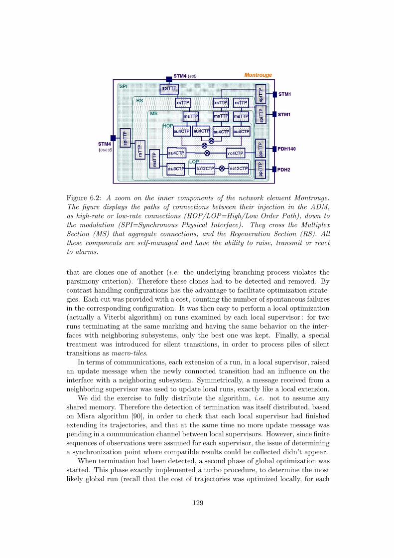
Figure 6.2: A zoom on the inner components of the network element Montrouge.The figure displays the paths of connections between their injection in the ADM,as high-rate or low-rate connections (HOP/LOP=High/Low Order Path), down tothe modulation (SPI=Synchronous Physical Interface). They cross the MultiplexSection (MS) that aggregate connections, and the Regeneration Section (RS). Allthese components are self-managed and have the ability to raise, transmit or reactto alarms.
that are clones one of another (i.e. the underlying branching process violates theparsimony criterion). Therefore these clones had to be detected and removed. Bycontrast handling configurations has the advantage to facilitate optimization strate-gies. Each cut was provided with a cost, counting the number of spontaneous failuresin the corresponding configuration. It was then easy to perform a local optimization(actually a Viterbi algorithm) on runs examined by each local supervisor : for tworuns terminating at the same marking and having the same behavior on the inter-faces with neighboring subsystems, only the best one was kept. Finally, a specialtreatment was introduced for silent transitions, in order to process piles of silenttransitions as macro-tiles.
In terms of communications, each extension of a run, in a local supervisor, raisedan update message when the newly connected transition had an influence on theinterface with a neighboring subsystem. Symmetrically, a message received from aneighboring supervisor was used to update local runs, exactly like a local extension.
We did the exercise to fully distribute the algorithm, i.e. not to assume anyshared memory. Therefore the detection of termination was itself distributed, basedon Misra algorithm [90], in order to check that each local supervisor had finishedextending its trajectories, and that at the same time no more update message waspending in a communication channel between local supervisors. However, since finitesequences of observations were assumed for each supervisor, the issue of determininga synchronization point where compatible results could be collected didn’t appear.
When termination had been detected, a second phase of global optimization wasstarted. This phase exactly implemented a turbo procedure, to determine the mostlikely global run (recall that the cost of trajectories was optimized locally, for each
129
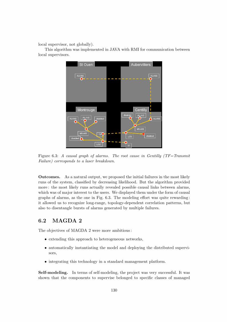
local supervisor, not globally).This algorithm was implemented in JAVA with RMI for communication between
local supervisors.
Figure 6.3: A causal graph of alarms. The root cause in Gentilly (TF=TransmitFailure) corresponds to a laser breakdown.
Outcomes. As a natural output, we proposed the initial failures in the most likelyruns of the system, classified by decreasing likelihood. But the algorithm providedmore : the most likely runs actually revealed possible causal links between alarms,which was of major interest to the users. We displayed them under the form of causalgraphs of alarms, as the one in Fig. 6.3. The modeling effort was quite rewarding :it allowed us to recognize long-range, topology-dependent correlation patterns, butalso to disentangle bursts of alarms generated by multiple failures.
6.2 MAGDA 2
The objectives of MAGDA 2 were more ambitious :
• extending this approach to heterogeneous networks,
• automatically instantiating the model and deploying the distributed supervi-sors,
• integrating this technology in a standard management platform.
Self-modeling. In terms of self-modeling, the project was very successful. It wasshown that the components to supervise belonged to specific classes of managed
130

objects. The latter can be found in the information model of the chosen networktechnology, and these information models are quite structured, Roughly speaking,they inherit their elements from common high level definitions of managed objects,like Trail/Connection Termination Point (TTP/CTP), Adaptation Layer, etc. So agreat part of the model structure is known : the modeler just has to specialize theseclasses to the target technology. This is true both for the managed components, fortheir connection capabilities, and for their behaviors : some behaviors are standardand can be described at a high level, like the transmission of messages betweencomponents, state changes in case of failure of a necessary function, the notion ofdependence of a service on another, etc.
A tool (OSCAR) was developed to allow a UML drawing of the model. This toolallowed us to draw a topology (deployment diagram), to read one in a file, and wasready to scan a network (which wasn’t experimented, however). It also allowed us torefine the managed objects, their connection capabilities, and to design elementarybehaviors (so-called tiles), with sequence diagrams. Finally, one could define withOSCAR the sub-systems associated to the different local supervisors.
Our application case in this project was a GMPLS/WDM network.
Figure 6.4: Correlated alarms, as they appeared in the management platform. Rootcauses were presented first, and the field “correlated notification flag” could be re-cursively clicked to discover immediate successors of an alarm.
Diagnosis technology. The computations were still based on configuration sets.The effort concentrated on the following features :
• The automatic deployment of the local supervisors. The latter were sent ondifferent machines, with knowledge of their sub-system model and of their
131

neighbors, connected together and initialized. This was programmed in Java+ CORBA.
• The distributed diagnosis algorithm was implemented above a rule engine,which is the standard correlation technology used in management platforms.We came up with three sets of rules : local extension rules, directly derivedfrom the sub-system model, optimization rules (specific to the management oftrajectories), and finally communication rules between local supervisors.
• The direct connection of local supervisors to a true management platform.Both to receive alarms from the platform, and to visualize their correlation atthe end of computations. This was done with CORBA.
Outcomes. Programming the distributed diagnosis algorithm over a rule enginewas a real challenge, but we proved its feasibility.
In terms of visualization of the results, we only selected the most likely explana-tion. We translated it into a causality graph between the received alarms, which wasused to fill the “correlated” field of alarms as they are stored in the managementplatform. This is illustrated in Fig. 6.4.
6.3 VDT
Figure 6.5: A submarine network, with several terminal equipment.
Objectives. VDT stands for Viterbi Diagnoser Technology. The objective of thiscontract was to propose an alarm correlation method for terminal equipment of sub-marine lines (SLTE, Fig. 6.5). These network elements aggregate in WDM trans-
132

missions high rate connections. They involve several layers of multiplexing andamplification, which results in quite complex systems, that can easily fill severalracks (Fig. 6.6). The objective was to correlate failure information propagating be-tween these functions. For example the fact that a low output signal of an amplifierwill cause extraction errors on all wavelengths multiplexed in this signal.
The major difficulty was that the propagation of failures were easy to describeat the physical level. Normally, this is where the redundancy of alarms should beavoided, by adequate masking procedures involving simple communications betweencards. Unfortunately, this feature is often considered as secondary, and deliverydelays generally prevent its development. So the correlation must be performedat the management level. There is no one-to-one mapping between the managedobjects and the underlying functions that support them. In general, a managedobject, like an Optical Path or an Optical Channel Group, collects information fromseveral cards, and symmetrically a failure on a given card is reflected in severalmanaged objects. Moreover, although alarms are non ambiguous at the physicallevel, they are translated (when they are) into very generic failure indications at themanagement level.
Specifying the system model at the management level was a real challenge. Nev-ertheless, we managed to recycle an important part of the self-modeling methodologydeveloped in Magda and Magda 2. A few components, specific to this technology,had to be designed, as well as specific connection capabilities. Behaviors were againextracted from failure scenarios given by an expert. And the counterpart of theOSCAR tool was redeveloped to easily draw the model.
Figure 6.6: Two submarine line terminal equipment (SLTE).
Diagnosis technology. This time we experimented a true unfolding-based ap-proach, in a centralized setting (a single supervisor). It was fed on one side by themodel produced by OSCAR, which was itself built from the description of an equip-ment architecture. On the other side, the diagnosis algorithm was fed by alarm logs,taking the form of a partial order (more precisely, a tuple of sequences). We exper-imented different unfolding algorithms. The most efficient was based on a recursivesub-routine to discover co-sets where a possible extension could be performed. Theunfolding was guided both by observations and by a cost function, in order to favor
133
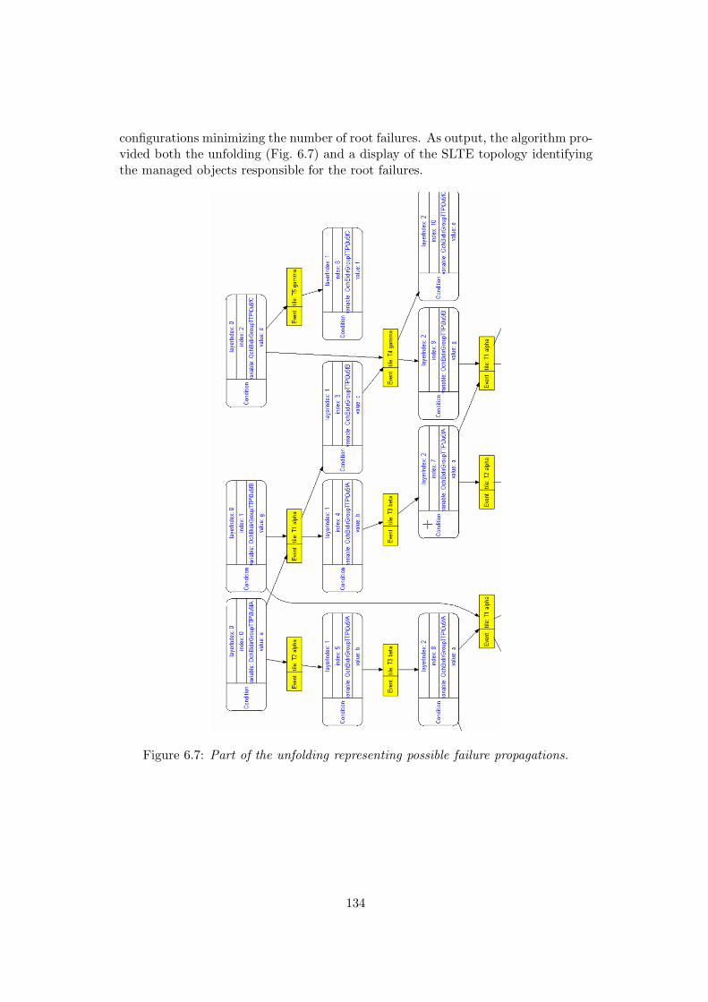
configurations minimizing the number of root failures. As output, the algorithm pro-vided both the unfolding (Fig. 6.7) and a display of the SLTE topology identifyingthe managed objects responsible for the root failures.
Figure 6.7: Part of the unfolding representing possible failure propagations.
134

Chapter 7
Conclusion
7.1 Summary of results
In substance, this document proposes a methodology to represent the trajectory setof a complex system, and an algebra to perform computations on these trajectories.We started by the definition of what we call complex systems : they are obtainedby assembling elementary components into a network, and thus can be describedas a graph of components. The time dimension is introduced by “unfolding” thesystem, in different ways, which is performed by a functor applied to the system.Many efforts have been dedicated to the design of such functors, in order to obtaintransformations that would preserve the interaction structure between components.So in all the proposed settings, runs of a compound system can be expressed asthe combination of runs of its components, which is called the “factorization prop-erty.” Formally, this property is equivalent to the factorization of the probabilitydistribution in a Markov random fields, which is itself the translation of conditionalindependence statements between components of the field (see the Hammersley-Clifford theorem). The analogy of these two domains has been established by meansof a common axiomatic framework. As a consequence, optimal estimation algo-rithms developed for Markov random fields (or Bayesian networks) can be recycledinto distributed asynchronous algorithms for networks of dynamic systems. Morespecifically, beyond factorization aspects, this formal analogy requires the existenceof a notion of projection that allows us to express a form of conditional independencestatement on trajectory sets (axiom (a3)).
The methodology presented in this document is very flexible and adapts to dif-ferent choices of trajectory semantics, and trajectory set representations. The twoarrays below summarize results.
In the case of sequential semantics, one can represent trajectory sets as a language(i.e. a collection of sequences), as a branching process (i.e. a decision tree), or as atrellis process, which extends the usual notion of trellis of an automaton. In all cases,these structures factorize into simpler factors, and there exists a natural notion ofprojection that allows us to implement message passing algorithms, for example tosolve the diagnosis problem. When runs are provided with costs, it is sometimespossible to use the MPA to perform an optimization task, for example to determine
135

Sequential semanticslanguage branching trellissystems processes processes
factorization property yes yes yesexistence of projections yes yes yesoptimization techniques yes yes ?
Figure 7.1: Available results for sequential semantics.
the global run of the system that minimizes the cost. We didn’t present it for trellisprocesses, whence the question mark, but this result seems accessible. It would takethe form of cooperating Viterbi algorithms, one per component, where several bestcost values (instead of one) would be carried by each state. They would correspondto the different synchronization patterns with neighboring components.
However, sequential semantics seem inappropriate for distributed systems : theygenerally induce large structures, whatever the representation one chooses. This isdue to two phenomena : first of all, the multi-clock feature, necessary to the factor-ization property, imposes large trellises, and secondly the natural concurrency thatarises in modular systems is not handled appropriately, which uselessly multipliesthe number of runs to consider. So the interest of sequential semantics is essen-tially theoretical : it provides a simple setting where the structure of distributedcomputations can be explained quite easily.
True concurrency semanticsMazurkiewicz traces branching trellis
(configurations) processes processesfactorization property yes yes yes
projections on a single variable yes yes yesexistence of general projections yes yes ?
optimization techniques yes ? ?
Figure 7.2: Available results for true concurrency semantics.
We rather recommend to use true concurrency semantics, that considerably re-duce the number of trajectories to consider, since the interleavings of concurrentevents are not computed. The three representations above remain possible. Insteadof languages, one has sets of configurations, or equivalently sets of Mazurkiewicztraces. Branching processes are now less trivial than simple decision trees : theybecome prefixes of the system unfolding, as it was defined for Petri nets. And fi-nally, we have also defined the appropriate notion of trellis process, an extensionof the notion of trellis to concurrent systems. Projections exist in almost all cases :they are easy to define when one projects on a simple system, with a single variable(and thus no possibility of internal concurrency). In the general case, one mustkeep track of some conflict and causality relations, which requires the more complexnotion of augmented configuration or augmented branching process. This generalprojection is still missing for trellis processes. Optimization techniques can also be
136

implemented on sets of traces : they look pretty much like those on languages. Butat this point it is not known whether they extend to the other structures.
7.2 Directions for future work
7.2.1 Technical extensions
The framework presented in this document may look quite complete and stable,but in reality many technical extensions demanded by applications remain openquestions. The most obvious ones are the empty entries in the previous arrays. Inparticular, a clear understanding of optimization issues is still missing. But severalother research directions deserve attention :
Label structures. The formal framework of chapter 2 is based on systems in-teracting by shared variables. But the computations we have presented, based oncompact encodings of trajectory sets, do not fit exactly this setting : interactionsare better described by shared labels, and projections on label sets are not (yet)defined. This motivated the use of pullbacks, to express component interactionsby means of shared variables/sites, i.e. interface automata. These representationsremain a bit unnatural because, in a pullback, the shared sites do not necessarilycapture all interactions between two components. Two ways to clarify this setting :either by re-expressing results of chapter 2 with a new formalism based on labelinteractions (in the spirit of the separation criterion appearing in theorem 9), or bydeveloping labeled event structures and a way to compose them with trajectory sets(as in section 3.4.2).
On-line computations. A nice algebraic translation of recursive algorithms inthe category theory setting is missing : what does it mean to replace an observedsequence by a longer one. Understanding this has important practical consequences :When one runs a recursive distributed diagnosis algorithm, messages are exchangedand new observations are introduced in a chaotic manner. One would like to deter-mine on-line which part of the local diagnoses computed so far are “stable” and canbe displayed. In the same way, where and how can we set a temporary stop point inthe algorithm to observe its current result. This certainly relates to the schedulingof operations in the algorithm, that was an unused degree of freedom so far. It alsorelates to “pure” aspects of distributed computing, as studied in [90].
Symbolic unfoldings. This idea was introduced by Thomas Chatain and ClaudeJard. Consider a “generic tile” t that would read the value of a state variable Vand add one to it. In the traditional construction of unfoldings, all values of Vwould appear as (conflicting) conditions, and the action of t would be connectedto each of them. In symbolic unfoldings, variable V appears only once, with anunknown value that depends on its past, and the action of t is represented as asymbolic event adding 1 to V . This results in much more compact structures. Theprice to pay is a more expensive test to decide whether a tile can be connected ornot. In order to compute with these objects, Thomas and I have already proved
137

that the factorization property still holds. It remains to build the adequate notionof projection. Let us mention that symbolic unfoldings are a natural tool to unfoldtime systems.
Multiresolution/hierarchical algorithms. The advantage of systems definedby constraints is that redundant constraints can only help reduction algorithms. Thepoint is to understand where ! One can suspect that extra long range constraintscould help to reach a better convergence of message passing algorithms (MPA). Onecould even imagine that well designed redundant components could help separatethe interaction graph into smaller parts. This is of course a model transformationissue, and there are probably resources about this question in the literature aboutdata-bases. Notice in particular that MPA are known in that field under the nameof query/sub-query algorithms.
Robustness issues. For our applications related to telecom networks, we havedeveloped a methodology to automatically build a model of the supervised network,by assembling generic components. In practice, a complete model is not alwaysavailable. One may only know parts of it, for example when a single domain ismonitored in a multi-domain architecture, or when a specific intermediate networklayer is monitored. Moreover, modeling errors may also introduce a mismatch be-tween what a model could produce, and what the system actually outputs. Finally,in the case of truly distributed algorithms, messages exchanged by local supervisorscould be lost, for example when the network management information is transmittedin-band. All these robustness issues have not been explored so far.
7.2.2 Research directions
Being able to compute efficiently on the trajectory set of a complex system poten-tially opens the way to numerous applications. We had distributed diagnosis issuesas our target, but several other domains seem accessible, or are worth being explored.Let us mention :
Smooth systems. This name suggests systems that have a non rigid interactionstructure. Networks can be reconfigured for example, create or kill connections,which amounts to creating or removing components in their model. In web services,the tree (or graph) of service requests, also called its choreography, may depend onthe parameters of the initial request or on the answer of some sub-services. Thesame phenomena appear with active XML documents (see the ASAX project). Thedifficulty here is not so much to define a notion of unfolding for such systems,where some transitions may create or disconnect components, but rather to proposea convenient model to describe the structural evolutions. Some partial answersalready exist, and there is hope to obtain factorization properties. But we are stillfar from applications.
Ad-hoc modeling. Related to modeling issues, another research direction con-cerns the extension of this work to other formalisms of concurrent systems. Scenario
138
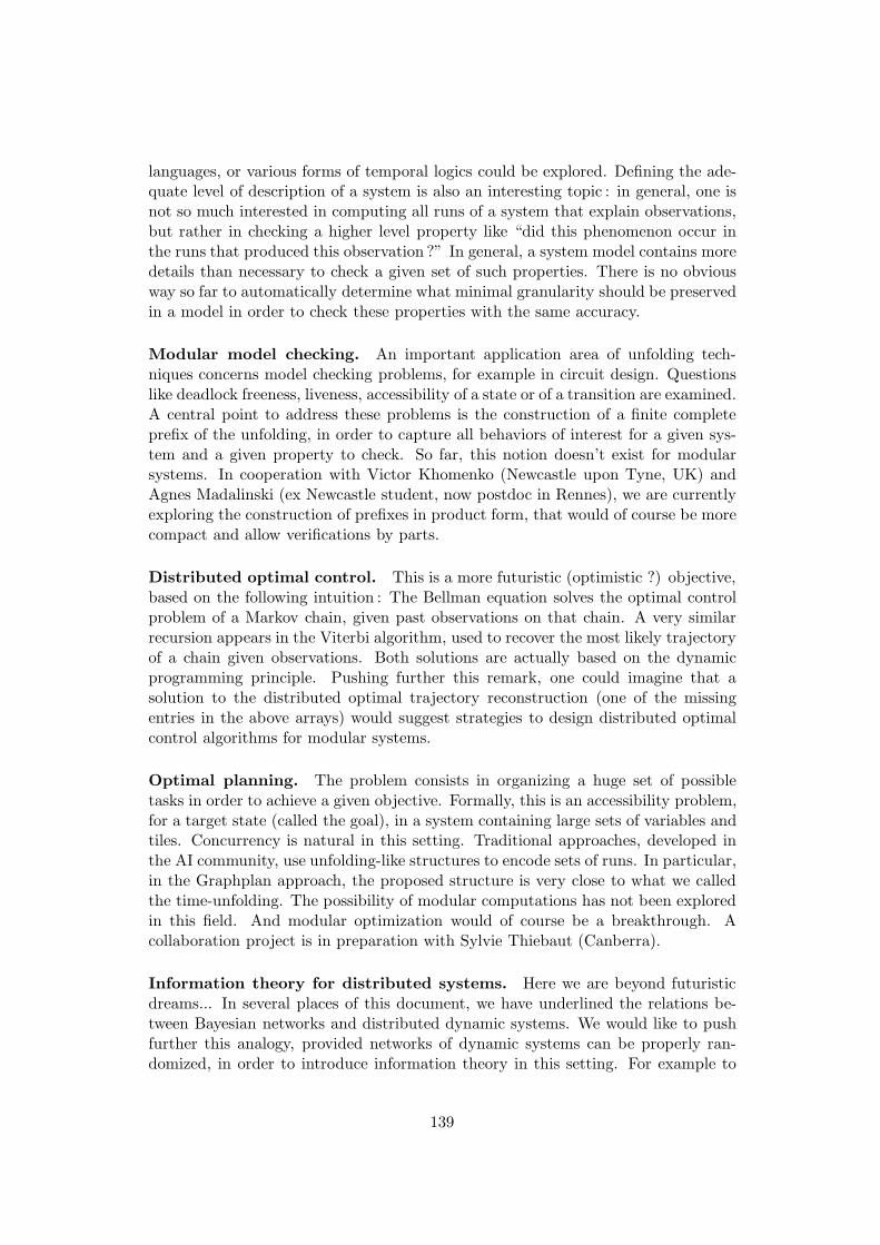
languages, or various forms of temporal logics could be explored. Defining the ade-quate level of description of a system is also an interesting topic : in general, one isnot so much interested in computing all runs of a system that explain observations,but rather in checking a higher level property like “did this phenomenon occur inthe runs that produced this observation ?” In general, a system model contains moredetails than necessary to check a given set of such properties. There is no obviousway so far to automatically determine what minimal granularity should be preservedin a model in order to check these properties with the same accuracy.
Modular model checking. An important application area of unfolding tech-niques concerns model checking problems, for example in circuit design. Questionslike deadlock freeness, liveness, accessibility of a state or of a transition are examined.A central point to address these problems is the construction of a finite completeprefix of the unfolding, in order to capture all behaviors of interest for a given sys-tem and a given property to check. So far, this notion doesn’t exist for modularsystems. In cooperation with Victor Khomenko (Newcastle upon Tyne, UK) andAgnes Madalinski (ex Newcastle student, now postdoc in Rennes), we are currentlyexploring the construction of prefixes in product form, that would of course be morecompact and allow verifications by parts.
Distributed optimal control. This is a more futuristic (optimistic ?) objective,based on the following intuition : The Bellman equation solves the optimal controlproblem of a Markov chain, given past observations on that chain. A very similarrecursion appears in the Viterbi algorithm, used to recover the most likely trajectoryof a chain given observations. Both solutions are actually based on the dynamicprogramming principle. Pushing further this remark, one could imagine that asolution to the distributed optimal trajectory reconstruction (one of the missingentries in the above arrays) would suggest strategies to design distributed optimalcontrol algorithms for modular systems.
Optimal planning. The problem consists in organizing a huge set of possibletasks in order to achieve a given objective. Formally, this is an accessibility problem,for a target state (called the goal), in a system containing large sets of variables andtiles. Concurrency is natural in this setting. Traditional approaches, developed inthe AI community, use unfolding-like structures to encode sets of runs. In particular,in the Graphplan approach, the proposed structure is very close to what we calledthe time-unfolding. The possibility of modular computations has not been exploredin this field. And modular optimization would of course be a breakthrough. Acollaboration project is in preparation with Sylvie Thiebaut (Canberra).
Information theory for distributed systems. Here we are beyond futuristicdreams... In several places of this document, we have underlined the relations be-tween Bayesian networks and distributed dynamic systems. We would like to pushfurther this analogy, provided networks of dynamic systems can be properly ran-domized, in order to introduce information theory in this setting. For example to
139

quantify the effect of a component on the others, evaluate the importance of a mes-sage in distributed algorithms, etc. This is probably a difficult task, given the poornumber of results available in network information theory, or in network coding.
140

Chapter 8
Acknowledgement
141


The School of Athens in Distributed Diagnosis
This picture was taken on June 14th, 2007, on the way out of IRISA’s confer-ence room, where the defense was taking place. Yes, we do have such magnificientrooms at IRISA, but we generally adopt a different dress code. Excepted on specialoccasions. That day was one of these occasions, as we were visited by many peopleof wisdom.
I am very indebted to Albert Benveniste, whom we see here,pointing his hand down to applications. I feel unable toexplain how much he supported this work. As a discov-erer of fruitful industrial problems, as a supporter of newapproaches to a problem, as a scientific reference, as a clar-ifier of confuse ideas, etc. My gratitute won’t find adequatewords.
This is Glynn Winskel, pointing his finger up to the idealworld of theoretical approaches, and carrying a copy of hisLecture Notes in Category Theory. I already mentioned howmuch his contributions have been inspiring for my work.I feel scientifically indebted to him, and honored that heaccepted to give his opinion on such non-standard uses offormal methods.
Alan Willsky, saying it’s highly time to go to the restaurant.Alan has the talent to conjugate a powerful scientific inspi-ration, with a deep and educated taste for the good aspectsof life. Visiting him at MIT has always been stimulatingon both topics ! His scientific enthousiasm is always a re-freshing pleasure, and I’m glad he accepted to evaluate mydeviating uses of belief propagation algorithms.
Nothing is as stimulating as a strong competitor. StephaneLafortune has laid a corner stone in diagnosis problems anddiagnosability issues, including distributed aspects. Afterseveral years of proximity in conference sessions, where youwait for his last novelties to nurture your own reflections,it’s a pleasure and a challenge to know his evaluation of adifferent point of view on the topic.
143

There are some people you’re always pleased to meetin a conference. Alessandro Giua is one of them, bothfor his pleasant company and for his wide culture incomputer science, Petri nets, discrete event systems,control... A challenge to have him as a reviewer.
Christophe Dousson has been our light house on in-dustrial problems for several years. He is himself acontributor to diagnosis solutions, and shared with ushis accurate perception about emerging technologiesand the problems they raised. Industrial partnershipshave been crucial to my work.
This is Michel Raynal, teaching. His books aboutdistributed computing helped me understand how tomake the joint between modular processings and trulydistributed algorithms. Among his (numerous) mottoCorrectness may be theoretical, but incorrectness has apractical impact. I’m honored he accepted to venturea bit outside his land to evaluate this document.
Your servant, exhausted.All this work for a parchment...
There are many other persons that directly or indirectly contributed to this work,as colleagues or as friends, with stimulating ideas, friendly support or love. Let mejust mention Armen Aghasaryan, and Claire. I’m sure the others will recognizethemselves on the picture.
144
Bibliography
[1] S. Abbes, “Probabilistic Models for Distributed and Concurrent Systems. Limit The-orems and Applications to Statistical Parametric Estimation,” PhD thesis no. 3026,IRISA, University of Rennes 1, Oct. 2004.
[2] S. Abbes, A. Benveniste, “Probabilistic models for true-concurrency : branching cellsand distributed probabilities for event structures,” Information & Computation 204(2),pp. 231-274, Feb. 2006.
[3] S. M. Aji, R. J. McEliece, “The Generalized Distributive Law,” IEEE Trans. Inform.Theory, vol. 46, no. 2 (March 2000), pp. 325-343.
[4] S. M. Aji, R. J. McEliece, “The Generalized Distributive Law and Free Energy Mini-mization,” 39th Allerton Conference, October 4, 2001.
[5] A. Aghasaryan, C. Dousson, ”Mixing Chronicle and Petri Net Approaches in EvolutionMonitoring Problems,” 12th workshop on Principles of Diagnosis (DX’01), pp. 1-7,March 2001.
[6] A. Arnold, “Finite Transition Systems,” Prentice Hall, 1992.
[7] P. Baldan, A. Corradini, H. Montanari, “Contextual Petri nets, asymmetric event struc-tures, and processes,” Information and Computation, Vol. 171(1), pp. 1-49, Nov. 2001.
[8] P. Baroni, G. Lamperti, P. Pogliano, M. Zanella, “Diagnosis of Large Active Systems,”Artificial Intell. 110, pp. 135-183, 1999.
[9] A. Benveniste, E. Fabre, S. Haar, C. Jard, “Diagnosis of asynchronous discrete eventsystems, a net unfolding approach,” IEEE Trans. on Automatic Control, vol. 48, no. 5,pp. 714-727, May 2003.
[10] C. Berrou, A. Glavieux, “Near optimum error correcting coding and decoding: turbo-codes,” In IEEE Trans. on Communications 44(10), Oct. 1996.
[11] S. Bibas, M.-O. Cordier, P. Dague, C. Dousson, F. Levy, L. Roze, “Alarm drivensupervision for telecommunication networks: I- Off-line scenario generation,” Annalsof Telecommunications n◦ 9/10 (tome 51),,pp. 493-500, Sept./Oct. 1996.
[12] A. Blum, M. Furst, “Fast Planning Through Planning Graph Analysis,” , ArtificialIntelligence, 90:281–300, 1997.
[13] R.K. Boel, J.H. van Schuppen, “Decentralized Failure Diagnosis for Discrete EventSystems with Costly Communication between Diagnosers,” in Proc. 6th Int. Workshopon Discrete Event Systems, WODES’02, pp. 175-181, 2002.
[14] R.K. Boel, G. Jiroveanu, “Distributed Contextual Diagnosis for very Large Systems,”in Proc. of WODES’04, pp. 343-348, 2004.
[15] C. Cassandras, S. Lafortune, “Introduction to Discrete Event Systems,” Kluwer Aca-demic Publishers, 1999.
145

[16] F. Cassez, T. Chatain, C. Jard, “Symbolic unfoldings for networks of timed automata,”In ATVA, LNCS 4218, pp. 307-321, 2006.
[17] I. Castellani, G.-Q. Zhang, “Parallel product of event structures,” Theoretical Com-puter Science, no. 179, pp. 203-215, 1997.
[18] T. Chatain, C. Jard, “Complete finite prefixes of symbolic unfoldings of safe time Petrinets,” ATPN’06, LNCS 4024, pp. 125-145, 2006.
[19] T. Chatain, “Symbolic Unfoldings of High-Level Petri Nets and Application to Super-vision of Distributed Systems,” PhD thesis, Universite de Rennes 1, November 2006.
[20] S.-Y. Chung, T. Richardson, R. Urbanke, “Analysis of Sum-Product Decoding of Low-Density Parity-Check Codes Using a Gaussian Approximation,” IEEE Trans. Inform.Theory, 47 (2001), pp. 657-670.
[21] O. Contant, S. Lafortune, “Diagnosis of Modular Discrete Event Systems,” in Proc. ofWODES’04, pp. 337-342, 2004.
[22] O. Contant, S. Lafortune, “Diagnosability of Discrete Event Systems with ModularStructure, J. of Discrete Event Dyn. Syst., vol. 16, pp. 9-37, 2006.
[23] J.-M. Couvreur, S. Grivet, D. Poitrenaud, “Unfolding of Products of SymmetricalPetri Nets,” 22nd International Conference on Applications and Theory of Petri Nets(ICATPN 2001), Newcastle upon Tyne, UK, June 2001, LNCS 2075, pp. 121-143.
[24] P. Darondeau, “Distributed implementations of Ramadge-Wonham supervisory controlwith Petri nets,” In 44th Conf. on Decision and Control (CDC), Seville, Spain, pp.2107-2112, December 2005.
[25] R. Debouk, S. Lafortune, D. Teneketzis, “Coordinated Decentralized Protocols forFailure Diagnosis of Discrete Event Systems,” Discrete Event Dynamic Systems,vol. 10(1/2), pp. 33-86, 2000.
[26] P. Degano, R. De Nicola, U. Montanari, “On the Consistency of Truly ConcurrentOperational and Denotational Semantics,” in proc. Symposium on Logic in ComputerScience (LICS) 1988, pp. 133-141.
[27] V. Diekert, G. Rozenberg, “The Book of Traces,” World Scientific Publishing, 1995.
[28] C. Dousson, “Alarm driven supervision for telecommunication networks: II- On-linechronicle recognition,” Annals of Telecommunications n◦ 9/10 (tome 51), pp. 501-508,Sept./Oct. 1996.
[29] C. Dousson, P. Le Maigat, “Chronicle Recognition Improvement Using Temporal Fo-cusing and Hierarchization,” 20th International Conference on Artificial Intelligence(IJCAI’07), pp. 324-329, Jan. 2007.
[30] C. Dousson, T. Vu Duong, “Discovering chronicles with numerical time constraintsfrom alarm logs for monitoring dynamic systems,” 16th IJCAI, pp. 620-626, Stockholm,Sweden, Aug. 99.
[31] J. Engelfriet, “Branching Processes of Petri Nets,” Acta Informatica no. 28, pp. 575-591, 1991.
[32] J. Esparza, “Model checking using net unfoldings,” Science of Computer Programming23, pp. 151-195, 1994.
[33] J. Esparza, S. Romer, W. Vogler, “An improvement of McMillan’s unfolding algo-rithm,” in Proc. of TACAS’96, LNCS 1055, pp. 87-106.
146

[34] J. Esparza, S. Romer, W. Vogler, “An Improvement of McMillan’s Unfolding Algo-rithm,” Formal Methods in System Design 20(3), pp. 285-310, May 2002. Extendedversion of [33].
[35] J. Esparza, S. Romer, “An unfolding algorithm for synchronous products of transitionsystems,” in Proc. of CONCUR’99, LNCS 1664, Springer Verlag, 1999.
[36] J. Esparza, C. Schroter, “Reachability Analysis Using Net Unfoldings,” Workshopof Concurrency, Specification and Programming, volume II of Informatik-Bericht 140,pp. 255-270, Humboldt-Universitat zu Berlin, 2000.
[37] E. Fabre, “Factorization of Unfoldings for Distributed Tile Systems, Part 1 : LimitedInteraction Case,” INRIA research report no. 4829, April 2003.
[38] E. Fabre, “Convergence of the turbo algorithm for systems defined by local con-straints,” INRIA research report no. PI 4860, May 2003.
[39] A. Benveniste, E. Fabre, S. Haar, “Markov Nets: Probabilistic Models for distributedand concurrent systems,” IEEE Transactions on Automatic Control, 48(11):1936-1950,November 2003.
[40] E. Fabre, “Factorization of Unfoldings for Distributed Tile Systems, Part 2 : GeneralCase,” INRIA research report no. 5186, May 2004.
[41] E. Fabre, A. Benveniste, S. Haar, C. Jard, “Distributed Monitoring of Concurrent andAsynchronous Systems,” Journal of Discrete Event Dynamic Systems, special issue,vol. 15 no. 1, pp. 33-84, March 2005.
[42] E. Fabre, “Distributed Diagnosis based on Trellis Processes,” In 44th Conf. on Decisionand Control (CDC), Seville, Spain, pp. 6329-6334, December 2005.
[43] E. Fabre, “On the Construction of Pullbacks for Safe Petri Nets,” In Applicationsand Theory of Petri Nets and other Models of Concurrency, ATPN’06, Turku, Finland,LNCS 4024, pp. 166-180, June 2006.
[44] E. Fabre, C. Hadjicostis, “A Trellis Notion for Distributed System Diagnosis with Se-quential Semantics,” In proc. 8th Int. Workshop on Discrete Events Systems, WODES,Ann Arbor, pp. 294-300, July 2006.
[45] E. Fabre, “Trellis Processes : a Compact Representation for Runs of Concurrent Sys-tems,” To appear in Journal of Discrete Event Dynamical Systems, 2007.
[46] E. Fabre, A. Benveniste, “Partial Order Techniques for Distributed Discrete EventSystems : Why You Can’t Avoid Using Them.” Plenary address presented by A. Ben-veniste, 8th Int. Workshop on Discrete Events Systems, WODES, Ann Arbor, pp. 1-2,July 2006.
[47] E. Fabre, A. Benveniste, “Partial Order Techniques for Distributed Discrete EventSystems : Why You Can’t Avoid Using Them.” INRIA Research Report RR 5916,May 2006, submitted to J. Discrete Event Dyn. Syst.
[48] E. Fabre, “Distributed system diagnosis with sequential semantics,” in preparation.
[49] F. Fessant, C. Dousson, F. Clerot, “Mining of a telecommunication alarm log to im-prove the discovery of frequent patterns,” Industrial Conf. on Data Mining (ICDM’04),Leipzig, Germany, July 2004.
[50] C.J. Fidge, “Logical time in distributed computing systems.” IEEE Computer 24(8),28–33, 1991.
147

[51] A. Giua, X. Xie, “Control of safe ordinary Petri nets with marking specifications usingunfolding,” Proc. IFAC WODES04: 7th Workshop on Discrete Event Systems (Reims,France), Sept. 2004.
[52] A. Giua, X. Xie, “Nonblocking control of Petri nets using unfolding,” 16th IFAC WorldCongress (Prague, Czech Republic), July 2005.
[53] A. Giua, X. Xie, “Control of safe ordinary Petri nets using unfolding,” J. of DiscreteEvent Dynamic Systems, Vol. 15(4), pp. 349-373, Dec. 2005.
[54] S. Genc, S. Lafortune, “Distributed Diagnosis of Discrete-Event Systems Using PetriNets,” in proc. 24th Int. Conf. on Applications and Theory of Petri Nets, LNCS 2679,pp. 316-336, June, 2003.
[55] S. Genc and S. Lafortune, “Distributed Diagnosis of Place-Bordered Petri Nets,” ac-cepted for publication to the IEEE Transactions on Automation Science and Engineer-ing, March 31, 2006.
[56] B. Guerraz, C. Dousson, “Chronicles Construction Starting from the Fault Model ofthe System to Diagnose,” Int. Workshop on Principles of Diagnosis (DX’04), pp. 51-56,Carcassonne, France, June 2004.
[57] A. Guyader, E. Fabre, C. Guillemot, M. Robert, “Joint source-channel turbo decod-ing of entropy-coded sources,” IEEE Journal on Selected Areas in Communications,Vol. 19(9), pp. 1680-1696, Sept. 2001.
[58] J Hagenauer, “The EXIT chart - Introduction to extrinsic information transfer initerative processing,” In Proc. 12th Eur. Signal Proc. Conf., EUSIPCO ’04, pp. 1541-1548, Vienna, Sept. 2004.
[59] K.X. He, M.D. Lemmon, “Liveness-Enforcing Supervision of Bounded Ordinary PetriNets using Partial Order Methods,” IEEE Trans. on Automatic Control, vol 47,pp. 1042-1055, July 2002.
[60] K. Heljanko, V. Khomenko, M. Koutny, “Parallelisation of the Petri Net UnfoldingAlgorithm,” 8th Int. Conf. on Tools and Algorithms for the Construction and Analysisof Systems (TACAS/ETAPS 2002), Grenoble, France, LNCS 2280 pp. 371-385, 2002.
[61] T. Jeron, H. Marchand, S. Pinchinat, M.-O. Cordier, “Supervision Patterns in DiscreteEvent Systems Diagnosis,” in proc. of WODES’06, pp. 262-268, Ann Arbor, July 10-12,2006.
[62] G. Jiroveanu, R. Boel, “Distributed Diagnosis for Petri Net models with unobserv-able interactions via common places,” 11th Conf. on Decision and Control (CDC’05,pp. 6305-6310, 2005.
[63] G. Jiroveanu, R. Boel, “Petri Net model-based Distributed Fault Diagnosis for largeInteracting Systems.” 16th Int. Workshop on Principles of Diagnosis (DX’05), pp. 25-30,2005.
[64] V. Khomenko, M. Koutny, W. Vogler, “Canonical Prefixes of Petri Net Unfoldings,”14th Int. Conf. on Computer Aided Verification (CAV 2002), Copenhagen, Denmark,LNCS 2404, pp. 582-595, 2002.
[65] V. Khomenko, M. Koutny, “LP Deadlock Checking Using Partial Order Dependencies,”11th Int. Conf. on Concurrency Theory (CONCUR 2000), University Park, Pennsylva-nia, USA, LNCS 1877, pp. 410-425, 2000.
148

[66] V. Khomenko, M. Koutny, “Towards an Efficient Algorithm for Unfolding PetriNets,” 12th Int. Conf. on Concurrency Theory (CONCUR 2001), Aalborg, Denmark,LNCS 2154, pp. 366-380, 2001.
[67] V. Khomenko, M. Koutny, W. Vogler, “Canonical Prefixes of Petri Net Unfoldings,”Acta Informatica, vol. 40, pp. 95-118, 2003
[68] V. Khomenko, A. Kondratyev, M. Koutny, W. Vogler, “Merged Processes - a NewCondensed Representation of Petri Net Behaviour,” Tech. Rep. Series CS-TR-884, Univ.of Newcastle upon Tyne, Jan. 2005.
[69] F. R. Kschischang, B. J. Frey, “Iterative Decoding of Compound Codes by ProbabilityPropagation in Graphical Models,” IEEE J. on Selected Areas in Communications,vol. 16(2), Feb. 1998, pp. 219-230.
[70] F. R. Kschischang, B. J. Frey, H.-A. Loeliger, “Factor Graphs and the Sum-ProductAlgorithm,” IEEE Transactions on Information Theory, vol. 47(2), Feb. 2001, pp. 498-519.
[71] G. Lamperti and M. Zanella. Diagnosis of discrete-event systems from uncertain tem-poral observations. Artif. Intell. 137(1-2): 91-163 (2002).
[72] G. Lamperti and M. Zanella. Diagnosis of Active Systems: Principles and Techniques.Kluwer International Series in Engineering and Computer Science, Vol. 741, 2003.
[73] G. Lamperti and M. Zanella. Flexible diagnosis of discrete-event systems by similarity-based reasoning techniques. Artif. Intell. 170(3): 232-297 (2006).
[74] G. Lamperti and M. Zanella. Incremental Processing of Temporal Observations in Su-pervision and Diagnosis of Discrete-Event Systems. ICEIS (2) 2006: 47-57.
[75] L. Lamport, N. Lynch, “Distributed Computing : Models and Methods,” in Hand-book of Theoretical Computer Science, vol. B : Formal Models and Semantics, Jan vanLeeuwen ed., Elsevier (1990), pp. 1157-1199.
[76] S. L. Lauritzen, D. J. Spiegelhalter, “Local computations with probabilities on graph-ical structures and their application to expert systems,” J. Royal Statistical Society,Series B, vol. 50(2), pp. 157-224, 1988.
[77] S. L. Lauritzen, “Graphical Models,” Oxford Statistical Science Series 17, OxfordUniversity Press, 1996.
[78] P. Le Maigat, C. Dousson, “Improvement of Chronicle-based Monitoring using Tem-poral Focalization and Hierarchization,” 17th International Workshop on Principles ofDiagnosis (DX’06), pp. 257-261, June 2006.
[79] R. J. McEliece, E. R. Rodemich, J.-F. Cheng, “ The Turbo Decision Algorithm,” 33rdAllerton Conf. on Communication, Control and Computing, Oct. 1995.
[80] R. J. McEliece, D. J. C. MacKay, J.-F. Cheng, “Turbo Decoding as an Instance ofPearl’s Belief Propagation Algorithm,” IEEE Journal on Selected Areas in Communi-cation, vol. 16(2), Feb. 1998, pp. 140-152.
[81] S. Mac Lane, “Categories for the Working Mathematician,” Springer-Verlag, 1971.
[82] K.L. McMillan, “Using unfoldings to avoid the state explosion problem in the verifica-tion of asynchronous circuits,” in Proc. 4th Workshop of Computer Aided Verification,Montreal, 1992, pp. 164-174.
[83] K.L. McMillan, “Symbolic Model Checking: An Approach to the State Explosion Prob-lem,” PhD thesis, Kluwer, 1993.
149

[84] F. Mattern. “Virtual time and global states of distributed systems,” Proc. Int. Work-shop on Parallel and Distributed Algorithms Bonas, France, Oct. 1988, Cosnard, Quin-ton, Raynal, and Robert Eds., North Holland, 1989.
[85] S. Melzer, S. Romer, “Deadlock checking using net unfoldings,” CAV’97, LNCS 1254,pp. 352-363.
[86] M. Nielsen, G. Plotkin, G. Winskel, “Petri nets, event structures and domains,” The-oretical Computer Science 13(1), 1981, pp. 85-108.
[87] J. Pearl, “Fusion, Propagation, and Structuring in Belief Networks,” Artificial Intelli-gence, vol. 29, pp. 241-288, 1986.
[88] Y. Pencole, M-O. Cordier, L. Roze, “A decentralized model-based diagnostic tool forcomplex systems,” Int. J. on Artif. Intel. Tools, World Scientific Publishing Comp.
[89] G. Provan, “A model-based diagnosis framework for distributed systems,” Int. Work-shop on Principles of Diagnosis (DX’02), 2002.
[90] M. Raynal, “Distributed algorithms and protocols,” Wiley & Sons, 1988
[91] W. Reisig, “Petri Nets,” Springer Verlag, 1985.
[92] T. Richardson, R. Urbanke, “The Capacity of Low-Density Parity Check Codes UnderMessage-Passing Decoding,” IEEE Trans. on Information Theory 47, pp. 599-618, Feb.2001.
[93] T. Richardson, R. Urbanke, “Design of capacity-approaching low density parity-checkcodes,” IEEE Trans. on Information Theory 47, pp. 619-637, Feb. 2001.
[94] T. Richardson, R. Urbanke, “An Introduction to the Analysis of Iterative CodingSystems,” In Codes, Systems, and Graphical Models, IMA Volume in Mathematicsand Its Applications, pages 1-37. Springer, 2001.
[95] M. Sampath, R. Sengupta, S. Lafortune, K. Sinnamohideen, D. Teneketzis, “Diagnos-ability of Discrete-event systems,” IEEE Trans. Autom. Control, vol. 40(9), pp. 1555-1575, 1995.
[96] M. Sampath, R. Sengupta, K. Sinnamohideen, S. Lafortune, D. Teneketzis, “Failurediagnosis using discrete event models,” IEEE Trans. on Systems Technology, vol. 4(2),pp. 105-124, March 1996.
[97] M. Steinder, A.S. Sethi, “End-to-End Service Failure Diagnosis Using Belief Networks,”Network Operations and Management Symposium (NOMS), Florence, Italy, 2002.
[98] M. Steinder, A.S. Sethi, “Distributed Fault Localization in Hierarchically Routed Net-works,” IFIP/IEEE Int. Workshop on Distributed Systems: Operations and Manage-ment (DSOM’02), LNCS 2506, pp. 195-207, 2002.
[99] E. Sudderth, M. Wainwright, A. Willsky, “Embedded Trees: Estimation of GaussianProcesses on Graph with Cycles,” IEEE Transactions on Signal Processing 52(11), Nov.2004.
[100] E. Sudderth, A. Ihler, W. Freeman, A. Willsky, “Nonparametric Belief Propagation,”IEEE Conference on Computer Vision and Pattern Recognition, June 2003.
[101] E. Sudderth, “Graphical Models for Visual Object Recognition and Tracking,” PhDThesis, Massachusetts Institute of Technology, May 2006.
[102] R. Su, “Distributed Diagnosis for Discrete-Event Systems,” PhD Thesis, Dept. ofElec. and Comp. Eng., Univ. of Toronto, June 2004.
150

[103] R. Su, W.M. Wonham, J. Kurien, X. Koutsoukos, “Distributed Diagnosis for Quali-tative Systems,” in Proc. 6th Int. Workshop on Discrete Event Systems, WODES’02,pp. 169-174, 2002.
[104] S. ten Brink, “Convergence behaviour of iteratively decoded parallel concatenatedcodes,” IEEE Trans. on Communications 49, Oct. 2001.
[105] S. Tripakis, “Undecidable Problems of Decentralized Observation and Control,” inProc. 40th Conf. on Decision and Control (CDC), 2001.
[106] F. W. Vaandrager, “A simple definition for parallel composition of prime eventsstructures,” Report CS-R8903, CWI, Amsterdam, March 1989.
[107] W. Vogler, A. Semenov, A. Yakovlev, “Unfolding and Finite Prefix for Nets with ReadArcs,” 9th Int. Conf. on Concurrency Theory (CONCUR), LNCS 1466, pp. 501-516,1998.
[108] Y. Weiss, W. T. Freeman, “On the Optimality of Solutions of the Max-Product Belief-Propagation Algorithm in Arbitrary Graphs,” IEEE Trans. on Information Theory,vol. 47, no. 2, pp. 723-735, Feb. 2001.
[109] G. Winskel, “A new Definition of Morphism on Petri Nets,” LNCS 166, pp. 140-149,1984.
[110] G. Winskel, “Categories of models for concurrency,” Seminar on Concurrency,Carnegie-Mellon Univ. (July 1984), LNCS 197, pp. 246-267, 1985.
[111] G. Winskel, “Event structure semantics of CCS and related languages,” LNCS 140,1982, also as report PB-159, Aarhus Univ., Denmark, April 1983.
[112] G. Winskel, “Petri Nets, Algebras, Morphisms, and Compositionality,” Informationand Computation, no. 72, pp. 197-238, 1997.
[113] J. S. Yedidia, W. T. Freeman, Y. Weiss, “Bethe free energy, Kikuchi approximations,and belief propagation algorithms,” available at www.merl.com/papers/TR2001-16/
[114] J. S. Yedidia, W. T. Freeman, Y. Weiss, “Generalized Belief Propagation,” Advancesin Neural Information Processing Systems (NIPS), Vol 13, pp. 689-695, December 2000,also as MERL Tech. Rep. no. TR2000-26.
[115] T. Yoo, S. Lafortune, “A General Architecture for Decentralized Supervisory Controlof Discrete-Event Systems,” J. Discrete Event Dynamic Systems: Theory and Applica-tions, vol. 12(3), pp. 335-377, July, 2002.
151