bayesian network constraint-based structure … network constraint-based structure learning...

JSS Journal of Statistical SoftwareMMMMMM YYYY, Volume VV, Issue II. http://www.jstatsoft.org/

Bayesian Network Constraint-Based Structure

Learning Algorithms: Parallel and Optimised

Implementations in the bnlearn R Package

Marco ScutariUniversity of Oxford

Abstract

It is well known in the literature that the problem of learning the structure of Bayesiannetworks is very hard to tackle: its computational complexity is super-exponential in thenumber of nodes in the worst case and polynomial in most real-world scenarios.

Efficient implementations of score-based structure learning benefit from past and cur-rent research in optimisation theory, which can be adapted to the task by using the net-work score as the objective function to maximise. This is not true for approaches basedon conditional independence tests, called constraint-based learning algorithms. The onlyoptimisation in widespread use, backtracking, leverages the symmetries implied by thedefinitions of neighbourhood and Markov blanket.

In this paper we illustrate how backtracking is implemented in recent versions of thebnlearn R package, and how it degrades the stability of Bayesian network structure learn-ing for little gain in terms of speed. As an alternative, we describe a software architectureand framework that can be used to parallelise constraint-based structure learning algo-rithms (also implemented in bnlearn) and we demonstrate its performance using fourreference networks and two real-world data sets from genetics and systems biology. Weshow that on modern multi-core or multiprocessor hardware parallel implementations arepreferable over backtracking, which was developed when single-processor machines werethe norm.

Keywords: Bayesian networks, structure learning, parallel programming, R.

1. Background and notations

Bayesian networks (BNs) are a class of graphical models (Pearl 1988; Koller and Friedman2009) composed by a set of random variables X = {Xi, i = 1, . . . ,m} and a directed acyclicgraph (DAG), denoted G = (V, A) where V is the node set and A is the arc set. The

arX

iv:1

406.

7648

v2 [

stat

.CO

] 1

Jun

201

5

http://www.jstatsoft.org/

2 Bayesian Network Learning: Parallel and Optimised Implementations

probability distribution of X is called the global distribution of the data, while those associatedwith individual Xis are called local distributions. Each node in V is associated with onevariable, and they are referred to interchangeably. The directed arcs in A that connectthem are denoted as “→” and represent direct stochastic dependencies; so if there is noarc connecting two nodes, the corresponding variables are either marginally independent orconditionally independent given (a subset of) the rest. As a result, each local distributiondepends only on a single node Xi and on its parents (i.e., the nodes Xj , j 6= i such thatXj → Xi, here denoted ΠXi):

P (X) =m∏i=1

P (Xi | ΠXi) . (1)

Common choices for the local and global distributions are multinomial variables (discreteBNs, Heckerman, Geiger, and Chickering 1995); univariate and multivariate normal variables(Gaussian BNs, Geiger and Heckerman 1994); and, less frequently, a combination of the two(conditional Gaussian (CG) BNs, Lauritzen and Wermuth 1989). In the first case, the param-eters of interest are the conditional probabilities associated with each variable, represented asconditional probability tables (CPTs); in the second, the parameters of interest are the partialcorrelation coefficients between each variable and its parents. As for CG BNs, the parametersof interest are again partial correlation coefficients, computed for each node conditional onits continuous parents for each configuration of the discrete parents.

The key advantage of the decomposition in Equation (1) is to make local computations possiblefor most tasks, using just a few variables at a time regardless of the magnitude of m. A relatedquantity that works to the same effect is the Markov blanket of each node Xi, defined as theset B(Xi) of nodes which graphically separates Xi from all other nodes V\{Xi,B(Xi)} (Pearl1988, p. 97). In BNs such a set is uniquely identified by the parents (ΠXi), the children (i.e.,the nodes Xj , j 6= i such that Xi → Xj) and the spouses of Xi (i.e., the nodes that share achild with Xi). By definition, Xi is independent of all other nodes given B(Xi), thus makingthem redundant for inference on Xi.

The task of fitting a BN is called learning and is generally implemented in two steps.

The first is called structure learning, and consists in finding the DAG that encodes the con-ditional independencies present in the data. This has been achieved in the literature withconstraint-based, score-based and hybrid algorithms; for an overview see Koller and Friedman(2009) and Scutari and Denis (2014). Constraint-based algorithms are based on the seminalwork of Pearl on causal graphical models and his Inductive Causation algorithm (IC, Vermaand Pearl 1991), which provides a framework for learning the DAG of a BN using condi-tional independence tests under the assumption that graphical separation and probabilisticindependence imply each other (the faithfulness assumption). Tests in common use are themutual information test (for discrete BNs) and the exact Student’s t test for correlation (forGBNs). Score-based algorithms represent an application of heuristic optimisation techniques:each candidate DAG is assigned a network score reflecting its goodness of fit, which the algo-rithm then attempts to maximise. BIC and posterior probabilities arising from various priorsare typical choices. Hybrid algorithms use both conditional independence tests and networkscores, the former to reduce the space of candidate DAGs and the latter to identify the op-timal DAG among them. Some examples are PC (named after its inventors Peter Spirtesand Clark Glymour; Spirtes, Glymour, and Scheines 2000), Grow-Shrink (GS; Margaritis

Journal of Statistical Software 3

2003), Incremental Association (IAMB; Tsamardinos, Aliferis, and Statnikov 2003), Inter-leaved IAMB (Inter-IAMB; Yaramakala and Margaritis 2005), hill-climbing and tabu search(Russell and Norvig 2009), Max-Min Parents & Children (MMPC; Tsamardinos, Brown, andAliferis 2006) and the Semi-Interleaved HITON-PC (SI-HITON-PC, from the Greek “hiton”for “blanket”; Aliferis, Statnikov, Tsamardinos, Mani, and Xenofon 2010). These algorithmsand more are implemented across several R packages, such as bnlearn (all of the above exceptPC; Scutari 2010), deal (hill-climbing; Bøttcher and Dethlefsen 2003), catnet and mugnet(simulated annealing; Balov and Salzman 2013; Balov 2013), pcalg (PC and causal graphicalmodel learning algorithms; Kalisch, Machler, Colombo, Maathuis, and Buhlmann 2012) andabn (hill climbing and exact algorithms; Lewis 2013). Further extensions to model dynamicdata are implemented in ebdbNet (Rau, Jaffrezic, Foulley, and Doerge 2010), G1DBN (Lebre2013) and ARTIVA (Lebre, Becq, Devaux, Lelandais, and Stumpf 2010) among others.

The second step is called parameter learning and, as the name suggests, deals with the esti-mation of the parameters of the global distribution. Since the graph structure is known fromthe previous step, this can be done efficiently by estimating the parameters of the local dis-tributions. With the exception of bnlearn, which has a separate bn.fit function, R packagesautomatically execute this step along with structure learning.

Most problems in BN theory have a computational complexity that, in the worst case, scalesexponentially with the number of variables. For instance, both structure learning (Chicker-ing 1996; Chickering, Geiger, and Heckerman 1994) and inference (Cooper 1990; Dagum andLuby 1993) are NP-hard and have polynomial complexity even for sparse networks. This isespecially problematic in high-dimensional settings such as genetics and systems biology, inwhich BNs are used for the analysis of gene expressions (Friedman 2004) and protein-proteininteractions (Jansen, Yu, Greenbaum, Kluger, Krogan, Chung, Emili, Snyder, Greenblatt,and Gerstein 2003; Sachs, Perez, Pe’er, Lauffenburger, and Nolan 2005); for integrating het-erogeneous genetic data (Chang and McGeachie 2011); and to determine disease susceptibilityto anemia (Sebastiani, Ramoni, Nolan, Baldwin, and Steinberg 2005) and hypertension (Mal-ovini, Nuzzo, Ferrazzi, Puca, and Bellazzi 2009).

Even though algorithms in recent literature are designed taking scalability into account, itis often impractical to learn BNs from data containing more than few hundreds of variableswithout restrictive assumptions on either the structure of the DAG or the nature of the localdistributions. Two ways to address this problem are:

1. optimisations: reducing the number of conditional independence tests and networkscores computed from the data, either by skipping redundant ones or by limiting localcomputations to a few variables;

2. parallel implementations: splitting learning across multiple cores and processors to makebetter use of modern multi-core and multiprocessor hardware.

As far as score-based learning algorithms are concerned, both possibilities have been exploredand a wide range of solutions proposed, from efficient caching using decomposable scores(Daly and Shen 2007), to parallel meta-heuristics (Rauber and Runger 2010) and integerprogramming (Cussens 2011). The same cannot be said of constraint-based algorithms; evenrecent ones such as SI-HITON-PC, while efficient, are still implemented with basic backtrack-ing as the only optimisation. We will examine them and their implementations in Section 2,arguing that backtracking provides only modest speed gains and increases the variability of


the learned DAGs. As an alternative, in Section 3 we describe a software architecture andframework that can be used to create parallel implementations of constraint-based algorithmsthat scale well on large data sets and do not suffer from this problem. In both sections wewill focus on the bnlearn package because it provides the widest choice of algorithms andimplementations among those of interest for this paper.

2. Constraint-based structure learning and backtracking

All constraint-based structure learning algorithms share a common three-phase structure in-herited from the IC algorithm through PC and GS; it is illustrated in Algorithm 1. The first,optional, phase consists in learning the Markov blanket of each node to reduce the numberof candidate DAGs early on. Any algorithm for learning Markov blankets can be plugged instep 1 and extended into a full BN structure learning algorithm, as originally suggested inMargaritis (2003) for GS. Once all Markov blankets have been learned, they are checked forconsistency (step 2) using their symmetry; by definition Xi ∈ B(Xj) ⇔ Xj ∈ B(Xi). Asym-metries are corrected by treating them as false positives and removing the offending nodesfrom each other’s Markov blankets.

The second phase learns the skeleton of the DAG, that is, it identifies which arcs are presentin the DAG modulo their direction. This is equivalent to learning the neighbours N (Xi) ofeach node: its parents and children. As illustrated in step 3, the absence of a set of nodesSXiXj that separates a particular pair Xi, Xj implies that either Xi → Xj or Xj → Xi.Separating sets are considered in order of increasing size to keep computations as local aspossible. Furthermore, if B(Xi) and B(Xj) are available from steps 1 and 2 the search spacecan be greatly reduced because N (Xi) ⊆ B(Xi). On the one hand, if Xj /∈ B(Xi) by definitionXi is separated from Xj by SXiXj = B(Xi). On the other hand, if Xj ∈ B(Xi) most candidatesets can be disregarded because we know that SXiXj ⊆ B(Xi) \Xj and SXiXj ⊆ B(Xj) \Xi;both sets are typically much smaller than V. With the exception of the PC algorithm, whichis structured exactly as described in step 3, constraint-based algorithms learn the skeleton bylearning each N (Xi) and then enforcing symmetry (step 4).

Finally, in the third phase arc directions are established as in Meek (1995). It is important tonote that, for some arcs, both directions are equivalent in the sense that they identify equiv-alent decompositions of the global distribution. Therefore, some arcs will be left undirectedand the algorithm will return a completed partially directed acyclic graph identifying an equiv-alence class containing multiple DAGs. Such a class is uniquely identified by the skeletonlearned in steps 3 and 4, and by the v-structures Vl of the form Xi → Xk ← Xj , Xi /∈ N (Xj)learned in step 5 (Chickering 1995). Additional arc directions are inferred indirectly in step6 by ruling out those that would introduce additional v-structures (which would have beenidentified in step 5) or cycles (which are not allowed in DAGs).

Even in such a general form, we can see that Algorithm 1 performs many checks for graphicalseparation that are redundant given the symmetry of the B(Xi) and the N (Xi). Intuitively,once we have concluded that Xj /∈ B(Xi) there is no need to check whether Xi ∈ B(Xj) instep 1; and similar considerations can be made for neighbours in step 3. In practice, thistranslates to redundant independence tests computed on the data. Therefore, up to version3.4 bnlearn implemented backtracking by assuming X1, . . . , Xm were processed sequentiallyand enforcing symmetry by construction (e.g., if i < j then Xj /∈ B(Xi) ⇒ Xi /∈ B(Xj) and


Algorithm 1 A template for constraint-based structure learning algorithms

Input: a data set containing the variables Xi, i = 1, . . . ,m.Output: a completed partially directed acyclic graph.

Phase 1: learning Markov blankets (optional).

1. For each variable Xi, learn its Markov blanket B(Xi).

2. Check whether the Markov blankets B(Xi) are symmetric, e.g., Xi ∈ B(Xj) ⇔ Xj ∈B(Xi). Assume that nodes for whom symmetry does not hold are false positives anddrop them from each other’s Markov blankets.

Phase 2: learning neighbours.

3. For each variable Xi, learn the set N (Xi) of its neighbours (i.e., the parents and thechildren of Xi). Equivalently, for each pair Xi, Xj , i 6= j search for a set SXiXj ⊂ V(including SXiXj = ∅) such that Xi and Xj are independent given SXiXj and Xi, Xj /∈SXiXj . If there is no such a set, place an undirected arc between Xi and Xj (Xi−Xj). IfB(Xi) and B(Xj) are available from points 1 and 2, the search for SXiXj can be limitedto the smallest of B(Xi) \Xj and B(Xj) \Xi.

4. Check whether the N (Xi) are symmetric, and correct asymmetries as in step 2.

Phase 3: learning arc directions.

5. For each pair of non-adjacent variables Xi and Xj with a common neighbour Xk, checkwhether Xk ∈ SXiXj . If not, set the direction of the arcs Xi − Xk and Xk − Xj toXi → Xk and Xk ← Xj to obtain a v-structure Vl = {Xi → Xk ← Xj}.

6. Set the direction of arcs that are still undirected by applying the following two rulesrecursively:

(a) If Xi is adjacent to Xj and there is a strictly directed path from Xi to Xj (a pathleading from Xi to Xj containing no undirected arcs) then set the direction ofXi −Xj to Xi → Xj .

(b) If Xi and Xj are not adjacent but Xi → Xk and Xk −Xj , then change the latterto Xk → Xj .

Xj ∈ B(Xi)⇒ Xi ∈ B(Xj)). While this approach on average reduces the number of tests by afactor of 2, it also introduces a false positive or a false negative in the learning process for everytype I or type II error in the independence tests. As long as BN learning was only feasiblefor simple data sets (due to limitations in computational power and algorithm efficiency),and the focus was on probabilistic modelling, the overall error rate was still acceptable; butthe increasing prevalence of causal modelling on “small n, large p” data sets in many fieldsrequires a better approach. One such is described in Tsamardinos et al. (2006, p. 46) andimplemented in bnlearn from version 3.5. It modifies steps 1 and 3 as follows:

• If Xj /∈ B(Xi), i < j, then do not consider Xi for inclusion in B(Xj); and if Xj /∈ N (Xi),


then do not consider Xi for inclusion in N (Xi).

• If Xj ∈ B(Xi) , then consider Xi for inclusion in B(Xj) by initialising B(Xj) = {Xi};and if Xj ∈ N (Xi) then initialise N (Xj) = {Xi}. Note that in both cases Xi can bediscarded in the process of learning B(Xj) and N (Xj).

Even in this form, backtracking has the undesirable effect of making structure learning dependon the order the variables are stored in the data set, which has been shown to increase errorsin the PC algorithm (Colombo and Maathuis 2013). In addition, backtracking provides onlya modest speed increase compared to a parallel implementation of steps 1-4; we will comparethe respective running times in Section 3. However, it is easy to implement side-by-side withthe original versions of constraint-based structure learning algorithms. Such algorithms aretypically described only at the node level, that is, they define how each B(Xi) and N (Xi)is learned and then they combine them as described in Algorithm 1. bnlearn exports twofunctions that give access to the corresponding backends: learn.mb to learn a single B(Xi) andlearn.nbr to learn a single N (Xi). The old approach to backtracking essentially whitelistedall nodes such that Xj ∈ B(Xi) and blacklisted all nodes such that Xj /∈ B(Xi) for each Xi.

R> library(bnlearn)

R> data(learning.test)

R> learn.nbr(x = learning.test, method = "si.hiton.pc", node = "D",

+ whitelist = c("A", "C"), blacklist = "B")

For example, in the code above we learn N (D) and, assuming we already learned N (A), N (B)and N (C), we whitelist and blacklist A, B and C depending on whether D was one of theirneighbours or not. The remaining nodes in the BN are neither whitelisted nor blacklisted andare then tested for conditional independence. By contrast, the current approach initialisesN (D) as {A, C} but does not whitelist those nodes.

R> learn.nbr(x = learning.test, method = "si.hiton.pc", node = "D",

+ blacklist = "B", start = c("A", "C"))

As a result, both A and C can be removed from N (D) by the algorithm. The vanilla, non-optimised equivalent for the same learning algorithm would be

R> learn.nbr(x = learning.test, method = "si.hiton.pc", node = "D")

which does not include any information from N (A), N (B) or N (C). The syntax for learn.mbis identical, and will be omitted for brevity. The only other R package implementing generalconstraint-based structure learning, pcalg, implements the PC algorithm as a monolithicfunction and does not export the backends which are used to learn the presence of an arcbetween a pair of nodes. Furthermore, as we noted above, PC is implemented differently fromother constraint-based algorithms and is usually modified with different optimisations thanbacktracking; see, for instance, the interleaving described in Colombo and Maathuis (2013).

In the remainder of this section we will focus on the effects of backtracking on learning theskeleton of the DAG, because steps 1-4 comprise the vast majority of the overall conditionalindependence tests and thus control most of the variability of the DAG. To investigate it, weused bnlearn and 5 reference BNs of various size and complexity from http://www.bnlearn.

com/bnrepository:

http://www.bnlearn.com/bnrepository

http://www.bnlearn.com/bnrepository


• ALARM (Beinlich, Suermondt, Chavez, and Cooper 1989), with 37 nodes, 46 arcs andp = 509 parameters. A BN designed by medical experts to provide an alarm messagesystem for intensive care unit patients based on the output a number of vital signsmonitoring devices.

• HEPAR II (Onisko 2003), with 70 nodes, 123 arcs and p = 1453 parameters. A BNmodel for the diagnosis of liver disorders from related clinical conditions (e.g., gallstones)and relevant biomarkers (e.g., bilirubin, hepatocellular markers).

• ANDES (Conati, Gertner, VanLehn, and Druzdzel 1997), with 223 nodes, 338 arcs andp = 1157 parameters. An intelligent tutoring system based on a student model for thefield of classical Newtonian physics, developed at the University of Pittsburgh and atthe United States Naval Academy. It handles long-term knowledge assessment, planrecognition, and prediction of students’ actions during problem solving exercises.

• LINK (Jensen and Kong 1999), with 724 nodes, 1125 arcs and p = 14211 parameters.Developed in the context of linkage analysis in large pedigrees, it models the linkageand the distance between a causal gene and a genetic marker.

• MUNIN (Andreassen, Jensen, Andersen, Falck, Kjærulff, Woldbye, Sørensen, Rosen-falck, and Jensen. 1989), with 1041 nodes, 1397 arcs with p = 80592 parameters. ABN designed by experts to interpret results from electromyographic examinations anddiagnose a large set of common diseases from physical conditions such as atrophy andactive nerve fibres.

Simulations were performed on a cluster of 7 dual AMD Opteron 6136, each with 16 cores and78GB of RAM, with R 3.1.0 and bnlearn 3.5. For each BN, we considered 6 different samplesizes (n = 0.1p, 0.2p, 0.5p, p, 2p, 5p), chosen as multiples of p to facilitate comparisons betweennetworks of such different complexity; and 4 different constraint-based structure learningalgorithms (GS, Inter-IAMB, MMPC, SI-HITON-PC). Since all reference BNs are discrete,we used the asymptotic χ2 mutual information test with α = 0.01. For each combinationof BN, sample size and algorithm we repeated the following simulation 20 times. First, weloaded the BN from the RDA file downloaded from the repository (alarm.rda below) andgenerated a sample of the appropriate size with rbn.

R> load("alarm.rda")

R> sim = rbn(bn, n = round(0.1 * nparams(bn)))

From that sample, we learned the skeleton of the DAG with (optimized = TRUE) and withoutbacktracking (optimized = FALSE).

R> skel.orig = skeleton(si.hiton.pc(sim, test = "mi", alpha = 0.01,

+ optimized = FALSE))

R> skel.back = skeleton(si.hiton.pc(sim, test = "mi", alpha = 0.01,

+ optimized = TRUE))

Subsequently, we reversed the order of the columns in the data to investigate whether thisresults in a different skeleton.

alarm.rda


Hamming distance

n/p

ALARM ANDES HEPAR II LINK MUNIN

SI−

HITO

N−

PC

MM

PC

Inter−IA

MB

GS

0.1

0.2

0.5

1.0

2.0

5.0

0 10 15 0 20 40 0 10 15 0 120 210 150 250 340

0.1

0.2

0.5

1.0

2.0

5.0

0 10 15 0 40 60 0 15 30 20 120 280 120 200 340

0.1

0.2

0.5

1.0

2.0

5.0

0 10 20 0 50 80 0 20 45 20 120 350 120 260 360

0.1

0.2

0.5

1.0

2.0

5.0

10 20 25 80 110 140 10 20 30 150 200 250 100 150 300

Figure 1: Hamming distance between skeletons learned for the ALARM, ANDES, HEPAR II,LINK and MUNIN reference BNs before and after reversing the ordering of the variables, forvarious n/p ratios and algorithms. Blue boxplots correspond to structure learning withoutbacktracking, green boxplots to learning with backtracking.


R> revsim = sim[, rev(seq(ncol(sim)))]

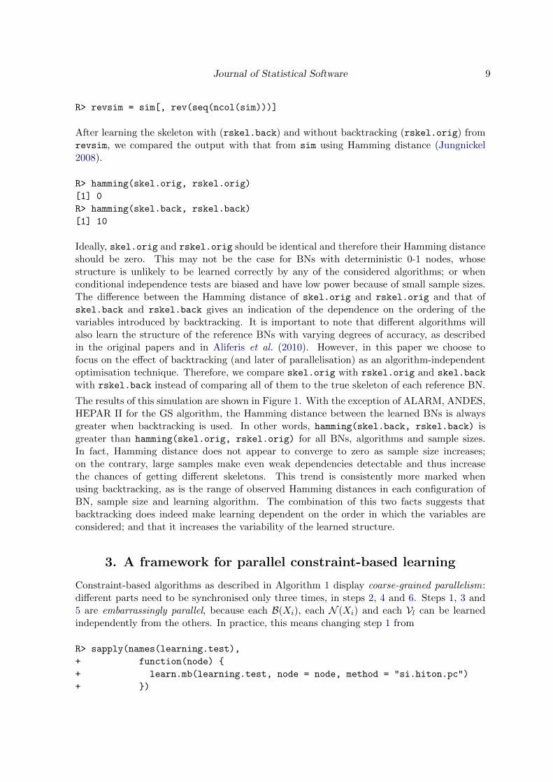
After learning the skeleton with (rskel.back) and without backtracking (rskel.orig) fromrevsim, we compared the output with that from sim using Hamming distance (Jungnickel2008).

R> hamming(skel.orig, rskel.orig)

[1] 0

R> hamming(skel.back, rskel.back)

[1] 10

Ideally, skel.orig and rskel.orig should be identical and therefore their Hamming distanceshould be zero. This may not be the case for BNs with deterministic 0-1 nodes, whosestructure is unlikely to be learned correctly by any of the considered algorithms; or whenconditional independence tests are biased and have low power because of small sample sizes.The difference between the Hamming distance of skel.orig and rskel.orig and that ofskel.back and rskel.back gives an indication of the dependence on the ordering of thevariables introduced by backtracking. It is important to note that different algorithms willalso learn the structure of the reference BNs with varying degrees of accuracy, as describedin the original papers and in Aliferis et al. (2010). However, in this paper we choose tofocus on the effect of backtracking (and later of parallelisation) as an algorithm-independentoptimisation technique. Therefore, we compare skel.orig with rskel.orig and skel.back

with rskel.back instead of comparing all of them to the true skeleton of each reference BN.

The results of this simulation are shown in Figure 1. With the exception of ALARM, ANDES,HEPAR II for the GS algorithm, the Hamming distance between the learned BNs is alwaysgreater when backtracking is used. In other words, hamming(skel.back, rskel.back) isgreater than hamming(skel.orig, rskel.orig) for all BNs, algorithms and sample sizes.In fact, Hamming distance does not appear to converge to zero as sample size increases;on the contrary, large samples make even weak dependencies detectable and thus increasethe chances of getting different skeletons. This trend is consistently more marked whenusing backtracking, as is the range of observed Hamming distances in each configuration ofBN, sample size and learning algorithm. The combination of this two facts suggests thatbacktracking does indeed make learning dependent on the order in which the variables areconsidered; and that it increases the variability of the learned structure.

3. A framework for parallel constraint-based learning

Constraint-based algorithms as described in Algorithm 1 display coarse-grained parallelism:different parts need to be synchronised only three times, in steps 2, 4 and 6. Steps 1, 3 and5 are embarrassingly parallel, because each B(Xi), each N (Xi) and each Vl can be learnedindependently from the others. In practice, this means changing step 1 from

R> sapply(names(learning.test),

+ function(node) {

+ learn.mb(learning.test, node = node, method = "si.hiton.pc")

+ })


directionpropagation

(step 6)

step 1 step 2 step 3 step 4 step 5

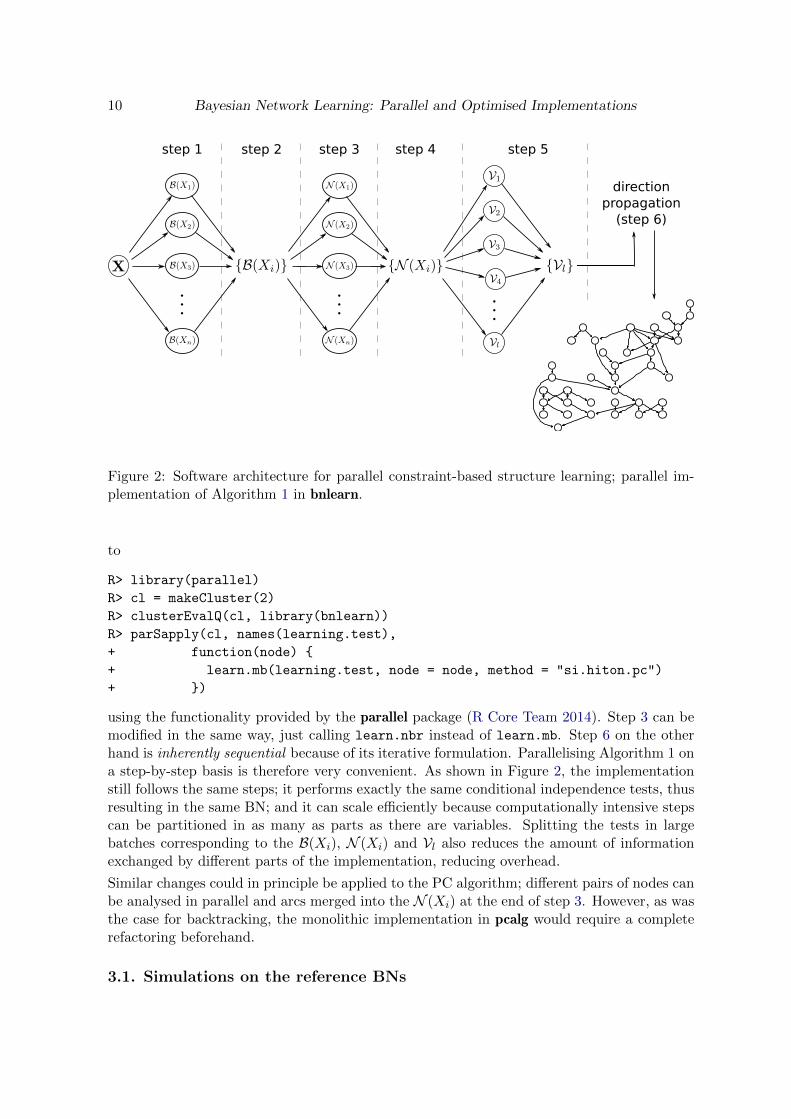
Figure 2: Software architecture for parallel constraint-based structure learning; parallel im-plementation of Algorithm 1 in bnlearn.

to

R> library(parallel)

R> cl = makeCluster(2)

R> clusterEvalQ(cl, library(bnlearn))

R> parSapply(cl, names(learning.test),

+ function(node) {

+ learn.mb(learning.test, node = node, method = "si.hiton.pc")

+ })

using the functionality provided by the parallel package (R Core Team 2014). Step 3 can bemodified in the same way, just calling learn.nbr instead of learn.mb. Step 6 on the otherhand is inherently sequential because of its iterative formulation. Parallelising Algorithm 1 ona step-by-step basis is therefore very convenient. As shown in Figure 2, the implementationstill follows the same steps; it performs exactly the same conditional independence tests, thusresulting in the same BN; and it can scale efficiently because computationally intensive stepscan be partitioned in as many as parts as there are variables. Splitting the tests in largebatches corresponding to the B(Xi), N (Xi) and Vl also reduces the amount of informationexchanged by different parts of the implementation, reducing overhead.

Similar changes could in principle be applied to the PC algorithm; different pairs of nodes canbe analysed in parallel and arcs merged into the N (Xi) at the end of step 3. However, as wasthe case for backtracking, the monolithic implementation in pcalg would require a completerefactoring beforehand.

3.1. Simulations on the reference BNs


All constraint-based learning algorithms in bnlearn have such a parallel implementation madeavailable transparently to the user, who only needs to initialise a cluster object using parallel.The master R process controls the learning process and distributes the B(Xi), N(Xi) and Vlto the slave processes, executing only steps 2, 4 and 6 itself. Consider, for example, theInter-IAMB algorithm and the data set generated from the ALARM reference BN shippedwith bnlearn.

R> data("alarm")

R> library("parallel")


R> res = inter.iamb(alarm, cluster = cl)

R> unlist(clusterEvalQ(cl, test.counter()))

[1] 3637 3743

R> stopCluster(cl)

After generating a cluster cl with 2 slave processes with makeCluster, we passed it tointer.iamb via the cluster argument. As we can see from the output of clusterEvalQ, thefirst slave process performed 3637 (49.3%) conditional tests, and the second 3743 (50.7%).The difference in the number of tests between the two slaves is due to the topology of the BN:the B(Xi) and N (Xi) have different sizes and therefore require different numbers of tests tolearn. This in turn also affects the number of tests required to learn the v-structures Vl.Increasing the number of slave processes reduces the number of tests performed by each ofthem, further increasing the overall performance of the algorithm.




[1] 2218 2479 2683

R> stopCluster(cl)




[1] 1737 1900 1719 2024

R> stopCluster(cl)

The raw and normalised running times of the algorithms used in Section 2 are reported inFigure 3 for clusters of 1, 2, 3, 4, 6 and 8 slaves; values are averaged over 10 runs for eachconfiguration using generated data sets of size 20000. Only the results for LINK and MUNINare shown, as they are the largest reference BNs considered in this paper. For ALARM,HEPAR II and ANDES, and for smaller sample sizes, running times are too short to makeparallel learning meaningful for at least MMPC and SI-HITON-PC. It is clear from the figurethat the gains in running time follow the law of diminishing returns: adding more slavesproduces smaller and smaller improvements. Furthermore, tests are never split uniformlyamong the slave processes and therefore slaves that have fewer tests to perform are left waitingfor others to complete (see, for instance, the R code snippets above). Even so, the parallelimplementations in bnlearn scale efficiently up to 8 slaves. In the absence of any overhead wewould expect the average normalised running time to be approximately 1/8 = 0.125; observed


MUNIN and LINK Reference Networks

number of slaves

norm

alis

ed r

unni

ng ti

me

LINK MUNIN

SI−

HITO

N−

PC

MM

PC

Inter−IA

MB

GS

10.

538

0.19

2

1 2 3 4 6 8

04:59

02:41

00:57

OPTIMISED: 05:16

10.

506

0.17

2

1 2 3 4 6 8

16:54

08:33

02:54

OPTIMISED: 16:40

10.

510.

181

1 2 3 4 6 8

04:38

02:21

00:50

OPTIMISED: 02:57

10.

496

0.16

5

1 2 3 4 6 8

14:23

07:08

02:22

OPTIMISED: 06:49

10.

498

0.15

1 2 3 4 6 8

36:48

18:20

05:31

OPTIMISED: 29:311

0.49

60.

166

1 2 3 4 6 8

30:52

15:18

05:08

OPTIMISED: 23:19

10.

512

0.15

7

1 2 3 4 6 8

28:38

14:39

04:29

OPTIMISED: 27:48

10.

572

0.19

1

1 2 3 4 6 8

25:59

14:51

04:57

OPTIMISED: 22:54

Figure 3: Normalised running times for learning the skeletons of the MUNIN and LINKreference BNs with the GS, Inter-IAMB, MMPC and SI-HITON-PC algorithms. Raw runningtimes are reported for backtracking and for parallel learning with 1, 2 and 8 slave processes.


Lung Adenocarcinoma

number of slaves

norm

alis

ed r

unni

ng ti

me

10.

521

0.37

70.

279

0.07

6

1 2 3 4 6 8 10 12 14 16 18 20

19:53:41

10:21:25

07:30:16

05:32:52

01:37:05

OPTIMISED: 09:33:54

WTCCC Heterogeneous Mice Population

number of slaves

norm

alis

ed r

unni

ng ti

me

1.00

00.

537

0.41

00.

300

0.06

2

1 2 3 4 6 8 10 12 14 16 18 20

08:09:53

04:22:54

03:20:42

02:27:03

00:34:05

OPTIMISED: 04:38:14

Figure 4: Running times for learning the skeletons underlying the lung adenocarcinoma (Beeret al. 2002) and mice (Valdar et al. 2006) data sets with SI-HITON-PC. Raw running timesare reported for backtracking and for parallel learning with 1, 2, 3, 4 and 20 slave processes.


values are in the range [0.157, 0.191]. The difference, which is in the range [0.032, 0.066], can beattributed to a combination of communication and synchronisation costs as discussed above.Optimised learning is at best competitive with 2 slaves (MMPC, MUNIN), and at worst mayactually degrade performance (LINK, SI-HITON-PC).

3.2. Simulations on the real-world data

To provide a more realistic benchmarking on large-scale biological data, we applied SI-HITON-PC on the lung adenocarcinoma gene expression data (86 observations, 7131 variables repre-senting expression levels) from Beer et al. (2002); and on the Wellcome Trust Case ControlConsortium (WTCCC) heterogeneous mice sequence data (1940 observations, 4053 variablesrepresenting allele counts) from Valdar et al. (2006). The former is a landmark study inpredicting patient survival after an early-stage lung adenocarcinoma diagnosis. Building agene network from such data to explore interactions and the presence of regulator genes isa common task in systems biology literature, hence the interest in benchmarking BN struc-ture learning. The latter is a reference data set produced by WTCCC to study genome-widehigh-resolution mapping of quantitative trait loci using mice as animal models for humandiseases. In this context BNs have been used to investigate dependence patterns betweensingle nucleotide polymorphisms (Morota, Valente, Rosa, Weigel, and Gianola 2012).

Both data sets are publicly available and have been preprocessed to remove highly correlatedvariables (COR > 0.95) and to impute missing values with the impute package (Hastie, Tib-shirani, Narasimhan, and Chu 2013). The adenocarcinoma data set has a sample size whichis extremely small compared to the number of variables, which is common in systems biology.On the other hand, the mice data has a sample size that is typical of large genome-wideassociation studies. We ran SI-HITON-PC using 1, 2, 3, 4, 6, 8, 10, 12, 14, 16, 18 and 20slaves, averaging over 5 runs in each case; the other algorithms we considered in Section 2did not scale well enough to handle either data set. Variables were treated as continuous, andindependence was tested using the Student’s t test for correlation with α = 0.01.

As we can see in Figure 4, we observe a low overhead even for 20 slave processes, withnormalised running times of 0.062 (mice) and 0.076 (adenocarcinoma) which are very close tothe theoretical 1/20 = 0.05. Similar considerations can be made across the whole range of 2to 20 slaves, with a measured overhead between 0.02 and 0.08. Surprisingly, overhead seemsto decrease in absolute terms with the number of slaves, from 0.04 (adenocarcinoma) and0.08 (mice) for 3 slaves to 0.012 (adenocarcinoma) and 0.026 (mice) for 20 slaves. However,clusters with 2 slaves have a smaller overhead (0.021 and 0.037) than those with 3 or 4 slaves.We note that overhead is comparable to that of the reference BNs in Section 2, suggesting thatit does not strongly depend on the size of the BN; and that the widely different sample sizesof the two data sets also seem to have little effect. Again, the running time of the optimisedimplementation is comparable with that of 2 slaves.

4. Discussion and conclusions

In this paper we described a software architecture and framework to create parallel imple-mentations of constraint-based structure learning algorithms for BNs and its implementationin bnlearn. Since all these algorithms trace their roots to the IC algorithm from Vermaand Pearl (1991), they share a common layout and can be parallelised in the same way. In


particular, several steps are embarrassingly parallel and can be trivially split in independentparts to be executed simultaneously. This is important for two reasons. Firstly, it limits theamount of overhead in the parallel computations due to the need of keeping different partsof the algorithms in sync. As we have seen in Section 3, this allows the parallel implemen-tations to scale efficiently in the number of slave processes. Secondly, it implies that theparallel implementation of each algorithm performs the same conditional independence testsas the original. This is in contrast with backtracking, which is the only widespread way ofimproving the sequential performance of constraint-based algorithms. Different approachesto backtracking have different speed-quality tradeoffs, which motivated the adoption of thatcurrently implemented in bnlearn. The simulations in Section 2 suggest that backtrackingcan increase the variability of the DAGs learned from the data. At the same time, speed gainsare competitive at most with the parallel implementation with 2 slave processes. Since mostcomputers in recent times come with at least 2 cores, it is possible to outperform backtrackingeven on commodity hardware while retaining the lower variability of the non-optimised imple-mentations. Furthermore, even for the largest number of processes considered in this paper (8for the reference BNs, 20 for the real-world data), the overhead introduced by communicationand synchronisation between the slaves is low; the highest observed value is 0.08. This sug-gests that the proposed software architecture as implemented in bnlearn and parallel scalesefficiently for the range of sample sizes and number variables considered in Section 3. Finally,it is important to note that these considerations arise from both discrete and Gaussian BNsand a variety of constraint-based structure learning algorithms.

As for future research, there are several possible ways in which the current implementationmay be studied and improved. First of all, overhead might be reduced by replacing parSapply

with a function that allocates the B(Xi) and N (Xi) dynamically to the slaves as they becomeidle. Assuming the underlying BN is sparse, which is often formalised with a bound on thesize of the B(Xi), this is likely to provide little practical benefit as the overhead is already lowcompared to the gains provided by parallelism. However, there are some specific settings suchas gene regulatory networks (e.g., Babu and Teichmann 2002) in which this assumption isknown not to hold; improvements may then be substantial. Such a setup could be based eitheron the mcparallel and mccollect functions in the parallel package, which unfortunately arenot available on Windows, or by avoiding parallel entirely to use the Rmpi package directly(Yu 2002). Synchronisation in steps 2 and 4 is required to obtain a consistent BN and thusprecludes the use of partial update techniques such as that described in Ahmed, Aly, Gonzalez,Narayanamurthy, and Smola (2012).

It would also be interesting to consider how the overhead scales in the sample size and inthe complexity of the BN. On average, the number of conditional independence tests requiredby constraint-based algorithms scales quadratically in the number of variables; and the teststhemselves are typically linear in complexity in the sample size. Increasing or decreasingthe latter should have little impact on the overhead of parallel learning, because data needto be copied only once to the slaves and that copy could be avoided altogether by using ashared-memory architecture. The results in Section 3.2 suggest this is indeed the case, andthe worst-case overhead is also similar to that of reference BNs in Section 3.1. No lockingor synchronisation is needed since the data are never modified by the algorithms. On theother hand, the number of variables in the BN can affect overhead in various ways. If theBN is small, differences in the learning times of the B(Xi) and N (Xi) are more likely to leaveslave processes idle even with the dynamic allocation scheme described above. However, if


the BN is large the size of the B(Xi) and N (Xi) may vary dramatically thus introducingsignificant overhead. In both cases the number of variables can only be used a rough proxyfor the complexity of the BN, which depends mainly on its topology; and imposing sparsityassumptions on the structure of the BN can be used as a tool to control overhead by keepingthe B(Xi) and N (Xi) small and of comparable size.

References

Ahmed A, Aly M, Gonzalez J, Narayanamurthy SM, Smola AJ (2012). “Scalable Inferencein Latent Variable Models.” In Proceeddings of the 5th ACM International Conference onWeb Search and Data Mining, pp. 123–132. ACM.

Aliferis CF, Statnikov A, Tsamardinos I, Mani S, Xenofon XD (2010). “Local Causal andMarkov Blanket Induction for Causal Discovery and Feature Selection for ClassificationPart I: Algorithms and Empirical Evaluation.” Journal of Machine Learning Research, 11,171–234.

Andreassen S, Jensen FV, Andersen SK, Falck B, Kjærulff U, Woldbye M, Sørensen AR,Rosenfalck A, Jensen F (1989). “MUNIN - an Expert EMG Assistant.” In Computer-AidedElectromyography and Expert Systems. Elsevier.

Babu MM, Teichmann SA (2002). “Evolution of Transcription Factors and the Gene Regula-tory Network in Escherichia Coli.” Nucleic Acids Research, 31(4), 1234–1244.

Balov N (2013). mugnet: Mixture of Gaussian Bayesian Network Model. R package version1.01.3.

Balov N, Salzman P (2013). catnet: Categorical Bayesian Network Inference. R packageversion 1.14.2.

Beer DG, Kardia SLR, Huang CC, Giordano TJ, Levin AM, Misek DE, Lin L, Chen G,Gharib TG, Thomas DG, Lizyness ML, Kuick R, Hayasaka S, Taylor JMG, IannettoniMD, Orringer MB, Hanash S (2002). “Gene-expression Profiles Predict Survival of Patientswith Lung Adenocarcinoma.” Nature Medicine, 8, 816–824.

Beinlich IA, Suermondt HJ, Chavez RM, Cooper GF (1989). “The ALARM MonitoringSystem: A Case Study with Two Probabilistic Inference Techniques for Belief Networks.”In J Hunter, J Cookson, J Wyatt (eds.), Proceedings of the 2nd European Conference onArtificial Intelligence in Medicine (AIME), pp. 247–256. Springer-Verlag.

Bøttcher SG, Dethlefsen C (2003). “deal: A Package for Learning Bayesian Networks.” Journalof Statistical Software, 8(20), 1–40.

Chang HH, McGeachie M (2011). “Phenotype Prediction by Integrative Network Analysis ofSNP and Gene Expression Microarrays.” In Proceedings of the 33rd Annual InternationalConference of the IEEE Engineering in Medicine and Biology Society (EMBC), pp. 6849–6852. IEEE Press, New York.


Chickering DM (1995). “A Transformational Characterization of Equivalent Bayesian NetworkStructures.” In Proceedings of the 11th Conference on Uncertainty in Artificial Intelligence(UAI95), pp. 87–98.

Chickering DM (1996). “Learning Bayesian Networks is NP-Complete.” In D Fisher, H Lenz(eds.), Learning from Data: Artificial Intelligence and Statistics V, pp. 121–130. Springer-Verlag.

Chickering DM, Geiger D, Heckerman D (1994). “Learning Bayesian Networks is NP-Hard.”Technical report, Microsoft Research, Redmond, Washington. Available as Technical ReportMSR-TR-94-17.

Colombo D, Maathuis MH (2013). “Order-independent Constraint-based Causal StructureLearning.” ArXiv preprint. URL http://arxiv.org/abs/1211.3295v2.

Conati C, Gertner AS, VanLehn K, Druzdzel MJ (1997). “On-line Student Modeling forCoached Problem Solving Using Bayesian Networks.” In A Jameson, C, C Tasso (eds.), InProceedings of the 6th International Conference on User Modeling, pp. 231–242. Springer-Verlag.

Cooper GF (1990). “The Computational Complexity of Probabilistic Inference Using BayesianBelief Networks.” Artificial Infelligence, 42(2–3), 393–405.

Cussens J (2011). “Bayesian Network Learning with Cutting Planes.” In FG Cozman, A Pfeffer(eds.), Proceedings of the 27th Conference on Uncertainty in Artificial Intelligence (UAI2011), pp. 153–160. AUAI Press.

Dagum P, Luby M (1993). “Approximating probabilistic inference in Bayesian belief networksis NP-Hard.” Artificial Intelligence, 60(1), 141–153.

Daly R, Shen Q (2007). “Methods to Accelerate the Learning of Bayesian Network Structures.”In Proceedings of the 2007 UK Workshop on Computational Intelligence. Imperial College,London.

Friedman N (2004). “Inferring Cellular Networks Using Probabilistic Graphical Models.”Science, 303(5659), 799–805.

Geiger D, Heckerman D (1994). “Learning Gaussian Networks.” Technical report, MicrosoftResearch, Redmond, Washington. Available as Technical Report MSR-TR-94-10.

Hastie T, Tibshirani R, Narasimhan B, Chu G (2013). impute: Imputation for MicroarrayData. R package version 1.36.0.

Heckerman D, Geiger D, Chickering DM (1995). “Learning Bayesian Networks: The Combi-nation of Knowledge and Statistical Data.” Machine Learning, 20(3), 197–243. Availableas Technical Report MSR-TR-94-09.

Jansen R, Yu H, Greenbaum D, Kluger Y, Krogan NJ, Chung S, Emili A, Snyder M, Green-blatt JF, Gerstein M (2003). “A Bayesian Networks Approach for Predicting Protein-Protein Interactions from Genomic Data.” Science, 302(5644), 449–453.

http://arxiv.org/abs/1211.3295v2


Jensen CS, Kong A (1999). “Blocking Gibbs Sampling for Linkage Analysis in Large Pedigreeswith Many Loops.” The American Journal of Human Genetics, 65(3), 885–901.

Jungnickel D (2008). Graphs, Networks and Algorithms. 3rd edition. Springer-Verlag.

Kalisch M, Machler M, Colombo D, Maathuis MH, Buhlmann P (2012). “Causal InferenceUsing Graphical Models with the R Package pcalg.” Journal of Statistical Software, 47(11),1–26.

Koller D, Friedman N (2009). Probabilistic Graphical Models: Principles and Techniques.MIT Press.

Lauritzen SL, Wermuth N (1989). “Graphical Models for Associations between Variables,some of which are Qualitative and some Quantitative.” The Annals of Statistics, 17(1),31–57.

Lebre S (2013). G1DBN: A Package Performing Dynamic Bayesian Network Inference. Rpackage version 3.1.1.

Lebre S, Becq J, Devaux F, Lelandais G, Stumpf M (2010). “Statistical Inference of theTime-Varying Structure of Gene-Regulation Networks.” BMC Systems Biology, 4(130),1–16.

Lewis F (2013). abn: Data Modelling with Additive Bayesian Networks. R package version0.83.

Malovini A, Nuzzo A, Ferrazzi F, Puca A, Bellazzi R (2009). “Phenotype Forecasting withSNPs Data Through Gene-Based Bayesian Networks.” BMC Bioinformatics, 10(Suppl 2),S7.

Margaritis D (2003). Learning Bayesian Network Model Structure from Data. Ph.D. thesis,School of Computer Science, Carnegie-Mellon University, Pittsburgh, PA. Available asTechnical Report CMU-CS-03-153.

Meek C (1995). “Causal Inference and Causal Explanation with Background Knowledge.” InP Besnard, S Hanks (eds.), Proceedings of the 11th Conference on Uncertainty in ArtificialIntelligence (UAI 2011), pp. 403–410. Morgan Kaufmann.

Morota G, Valente BD, Rosa GJM, Weigel KA, Gianola D (2012). “An Assessment of LinkageDisequilibrium in Holstein Cattle Using a Bayesian Network.” Journal of Animal Breedingand Genetics, 129(6), 474–487.

Onisko A (2003). Probabilistic Causal Models in Medicine: Application to Diagnosis of LiverDisorders. Ph.D. thesis, Institute of Biocybernetics and Biomedical Engineering, PolishAcademy of Science, Warsaw.

Pearl J (1988). Probabilistic Reasoning in Intelligent Systems: Networks of Plausible Infer-ence. Morgan Kaufmann.

R Core Team (2014). R: A Language and Environment for Statistical Computing. R Founda-tion for Statistical Computing, Vienna, Austria. URL http://www.R-project.org/.

http://www.R-project.org/


Rau A, Jaffrezic F, Foulley JL, Doerge R (2010). “An empirical Bayesian method for es-timating biological networks from temporal microarray data.” Statistical Applications inGenetics and Molecular Biology, 9(1).

Rauber T, Runger G (2010). Parallel Programming For Multicore and Cluster Systems.Springer-Verlag.

Russell SJ, Norvig P (2009). Artificial Intelligence: A Modern Approach. 3rd edition. PrenticeHall.

Sachs K, Perez O, Pe’er D, Lauffenburger DA, Nolan GP (2005). “Causal Protein-SignalingNetworks Derived from Multiparameter Single-Cell Data.” Science, 308(5721), 523–529.

Scutari M (2010). “Learning Bayesian Networks with the bnlearn R Package.” Journal ofStatistical Software, 35(3), 1–22.

Scutari M, Denis JB (2014). Bayesian Networks with Examples in R. Chapman & Hall.

Sebastiani P, Ramoni MF, Nolan V, Baldwin CT, Steinberg M (2005). “Genetic Dissectionand Prognostic Modeling of Overt Stroke in Sickle Cell Anemia.” Nature Genetics., 37(4),435–440.

Spirtes P, Glymour C, Scheines R (2000). Causation, Prediction, and Search. MIT Press.

Tsamardinos I, Aliferis CF, Statnikov A (2003). “Algorithms for Large Scale Markov BlanketDiscovery.” In I Russell, SM Haller (eds.), Proceedings of the 16th International FloridaArtificial Intelligence Research Society Conference, pp. 376–381. AAAI Press.

Tsamardinos I, Brown LE, Aliferis CF (2006). “The Max-Min Hill-Climbing Bayesian NetworkStructure Learning Algorithm.” Machine Learning, 65(1), 31–78.

Valdar W, Solberg LC, Gauguier D, Burnett S, Klenerman P, Cookson WO, Taylor MS,Rawlins JN, Mott R, Flint J (2006). “Genome-Wide Genetic Association of Complex Traitsin Heterogeneous Stock Mice.” Nature Genetics, 8, 879–887.

Verma TS, Pearl J (1991). “Equivalence and Synthesis of Causal Models.” Uncertainty inArtificial Intelligence, 6, 255–268.

Yaramakala S, Margaritis D (2005). “Speculative Markov Blanket Discovery for OptimalFeature Selection.” In ICDM ’05: Proceedings of the Fifth IEEE International Conferenceon Data Mining, pp. 809–812. IEEE Computer Society.

Yu H (2002). “Rmpi: Parallel Statistical Computing in R.” R News, 2(2), 10–14.


Affiliation:

Marco ScutariDepartment of StatisticsUniversity of Oxford1 South Parks RoadOX1 3TG Oxford, United KingdomE-mail: [email protected]: http://www.bnlearn.com/about

Journal of Statistical Software http://www.jstatsoft.org/

published by the American Statistical Association http://www.amstat.org/

Volume VV, Issue II Submitted: yyyy-mm-ddMMMMMM YYYY Accepted: yyyy-mm-dd

mailto:[email protected]

http://www.bnlearn.com/about

http://www.jstatsoft.org/

http://www.amstat.org/

bayesian network constraint-based structure … network constraint-based structure learning...

Documents