Bayesian models and simulations

in cognitive science

Giuseppe Boccignone1, Roberto Cordeschi2

1Natural Computation LabDipartimento di Ing.dell’Informazione e Ing. Elettrica

Universita di Salernovia Ponte Melillo, 1 -84084 Fisciano (SA), Italy

boccig@unisa.it

2Dipartimento di Studi Filosofici ed EpistemologiciUniversita di Roma ”La Sapienza”

via Carlo Fea 2, I-00161 Roma, Italycordeschi@caspur.it

Abstract

Bayesian models can be related to cognitive processes in a variety of

ways that can be usefully understood in terms of Marr’s distinction among

three levels of explanation: computational, algorithmic and implementa-

tion. In this note, we discuss how an integrated probabilistic account of

the different levels of explanation in cognitive science is resulting, at least

for the current research practice, in a sort of unpredicted epistemological

shift with respect to Marr’s original proposal.

1 Introduction

Sophisticated probabilistic models are finding increasingly wide application acrossthe cognitive and brain sciences.

It has been argued [Knill et al., 1996, Chater et al., 2006] that probabilisticmodels can be related to cognitive processes in a variety of ways. This varietycan be usefully understood in terms of Marr’s [1982] widely known distinctionbetween three levels at which any agent carrying out a task must be under-stood, the what/why level (computational theory), the how level (algorithm),the physical realization (implementation):

• Computational theory. What is the goal of the computation, why is itappropriate, and what is the logic of the strategy by which it can becarried out?

1

• Representation and algorithm. How can the computational theory be im-plemented? What is the representation for the input and output, andwhat is the algorithm for the transformation?

• Implementation. How can the representation and algorithm be realizedphysically?

Figure 1: The three levels of explanation suggested by Marr.

Indeed, in research work on theoretical foundations of cognitive scienceMarr’s account has become a sort of paradigm.

In this note, we discuss how an integrated probabilistic account of the differ-ent levels of explanation in cognitive science is resulting, at least for the currentresearch practice, in a sort of unpredicted epistemological shift with respect toMarr’s original proposal.

From a broader viewpoint such account can be seen as a tenet of philosophyof science that complex systems are to be seen as typically having multiple levelsof organization. The behavior of a complex system, e.g., a particular organism,might be explained at various levels of organization, including (but not restrictedto) ones which are biochemical, cellular, neurological, psychological.

Although Marr referred to the highest level of analysis as a theory, theterm model [Giere, 2004] is more appropriate: the cognitive scientist uses modelM to represent an aspect of the world W for purposes P (for details on thedevelopment of the concept of model from cybernetics to cognitive science, seeCordeschi [2002]). So, in the following we will refer to this level as the level of thecomputational model. In general, M could be many things, but Marr is easilyrecognized as addressing a kind of theoretical model [Giere, 2004, Hartmann andFrigg, 2005].

2

The intermediate level of analysis can be considered as a computer simula-tion, in the sense of Hartmann [2005], but constrained by model M.

The lowest level is that of the device in which the process is to be phys-ically realized. Clearly, if natural cognition is the focus, then neurophysiol-ogy/neuroanatomy is the level that should be addressed.

2 Bayesian explanations

In Chater et al. [2006] and Knill et al. [1996], the Bayesian framework is usedto formalize Marr’s three-fold hierarchy in two levels: the computational leveland the implementation level (embedding both Marr’s algorithmic and physicalrealization levels).

Figure 2: The levels of explanation according to Yuille and Kersten (adaptedfrom [Knill et al., 1996]).

Interestingly enough, both levels are denoted ”theories” [Chater et al., 2006]and, differently from Marr, a tight interaction between computational (hereBayesian) theory and implementation theory is assumed.

Beyond such claims and independently of methodological issues, current re-search practice in Bayesian cognition seems to reflect and widen such epistemo-logical shift.

Much cognitive processing is naturally interpreted as uncertain inferencewhich can be shaped by probabilistic methods at the computational level. Atsuch level the Bayesian framework is exploited to specify the so called generativemodel, via the joint probability density function (pdf).

The joint pdf P ({Xk}Kk=1) of the random variables (RVs) X1, · · · , XK is

defined and constraints accounted for through a graphical model GM (e.g., aBayesian network, or a Markov Random Field), an iconic representation of RVsdependencies where each node of the graph represents a RV, and arrows denoteconditional dependencies between variables.

3

To make this point clear, consider the following example (a similar one isdiscussed in Kersten and Yuille [2003]). We want to model the ability of thevisual system in recognizing that the object represented in the two images shownin Fig. 3 is one and the same despite considerable image variation caused by aviewpoint change (object invariance).

Figure 3: The same object seen under different views.

More precisely, the issue here is to make a decision about the object O,when the image I being observed takes the value I∗ (this is also known asthe evidence), while discounting the ”noisy” change of view V ; in probabilisticterms, the problem amounts to infer the marginal probability P (O|I = I∗).

Thus, knowledge is represented by the joint probability P (O, V, I). Notethat such pdf is symmetrical with respect to the three variables O, V, I. In factany three variable distribution P (X1, X2, X3) may be written, by application ofproduct rule of probability, in any of the 6 ways

P (Xi1 |Xi2 , Xi3)P (Xi2 |Xi3)P (Xi3 )

where (i1, i2, i3) is any of the 6 permutations of (1, 2, 3). Hence, whilst allgraphically different, they all represent the same distribution which does notmake any conditional independence statements.

In the example we are considering, we can assume that the data I are de-termined (generated) by the object O plus a possible view change V ; further, itis plausible to assume that the target object O does not directly influence theset of possible views V , neither views affect object model O (conditional inde-pendence P (O, V ) = P (O)P (V )). In other terms, the problem at hand suggesta joint probability decomposition of the type

P (O, V, I) = P (I|O, V )P (O, V ) = P (I|O, V )P (O)P (V ) (1)

whose equivalent iconic representation is the graph GM = {(O, V ) → I}. Thus,the generative model of object appearance under a change of view can be de-picted as in Fig. 4.

(A common practice is to work the way round: design the graph structurethat best represent the addressed problem, and then straightforwardly turn suchrepresentation in the corresponding joint pdf decomposition).

Recall that we want to infer the marginal probability P (O|I = I∗) giventhe evidence (observation) I = I∗. For simplicity, assume that probabilitiesP (I|O, V ), P (O), P (V ) specifying the generative model in Eq. 1 are actuallyknown, either in parametric form or in terms of conditional probability tables.

4

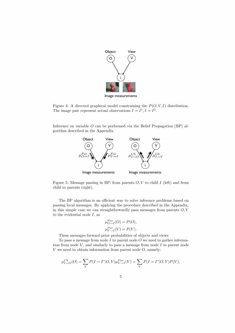
Figure 4: A directed graphical model constraining the P (O, V, I) distribution.The image pair represent actual observations I = I1, I = I2.

Inference on variable O can be performed via the Belief Propagation (BP) al-gorithm described in the Appendix.

Figure 5: Message passing in BP: from parents O, V to child I (left) and fromchild to parents (right).

The BP algorithm is an efficient way to solve inference problems based onpassing local messages. By applying the procedure described in the Appendix,in this simple case we can straightforwardly pass messages from parents O, V

to the evidential node I, as

µParO→I(O) = P (O),

µParV →I(V ) = P (V ).

These messages forward prior probabilities of objects and viewsTo pass a message from node I to parent node O we need to gather informa-

tion from node V , and similarly to pass a message from node I to parent nodeV we need to obtain information from parent node O, namely:

µChI→O(O) =

∑

V

P (I = I∗|O, V )µParV →I(V ) =

∑

V

P (I = I∗|O, V )P (V ),

5

µChI→V (V ) =

∑

O

P (I = I∗|O, V )µParO→I(O) =

∑

O

P (I = I∗|O, V )P (O).

Note that∑

X P (X) denotes a sum with respect to values taken by RV X , e.g.,P (X = x1) + P (X = x2) + P (X = x3).

Eventually the probability P (O|evidence) can be approximated as:

P (O|I = I∗) ∝ P (O) ·∑

V

P (I = I∗|O, V )P (V ). (2)

Summing up, the (Bayesian) computational model can be precisely definedas the pair M = 〈P ({Xk}

Kk=1),GM〉 (and, obviously, by exactly specifying the

form/parameters of conditional distributions)Model M together with probabilistic calculus, could in principle be used

for Bayesian inference and estimating any variable Xk. Note that by infer-ence we simply mean the computation of these marginal probabilities (beliefs).It is worth noting that for a small Bayesian network as that used before, wecould have easily performed direct marginalization. However, when scaled-up to real-world problems, exact Bayesian computations are intractable andapproximate algorithms have been developed for both learning and inference(e.g., the Expectation-Maximization algorithm, the Belief Propagation algo-rithm [MacKay, 2004, Lee and Mumford, 2003], and also Appendix A). Thevirtue of the BP algorithm is that we can use it to compute approximatemarginal probabilities in a time that grows only linearly with the number ofnodes in the system. In this perspective BP can be properly considered as asimulation of the inference process in the sense of Winsberg [2004]. In otherterms, Marr’s algorithmic level now performs a computer simulation by usingthe GM as a representation (data structure).

Eventually, for what concerns Marr’s implementation level, current debateis focusing on whether the brain itself should be viewed in probabilistic termsand the nervous system as implementing probabilistic calculations [Lee andMumford, 2003, Kersten and Yuille, 2003, Paulin, 2005]. This issue will becomeevident in the case study presented in the following Section.

3 A case study

One clear and elegant example of Bayesian methodology is provided by Rao[2005] who addresses the issue that neurons in cortical areas V2 and V4 can bemodulated by attention to particular locations of an image I (the retinal input).

According to the classical what/where model [Mishkin et al., 1983], Raoassumes that neurons in V4 area encode feature F (preferred stimulus) whilespatial locations L are encoded within the parietal cortex area; V1 and V2 areasplay the role of encoding an intermediate representation, say C.

6

The hierarchical organization of visual attention processing is summarizedin Fig. 6. The same figure shows the corresponding graphical model, whereF, L, C, I play the role of random variables.

Figure 6: The underlying hierarchical neural architecture (top) supporting vi-sual attention and the corresponding graphical model (bottom).

Marr’s levels of explanations for such a problem can be restated as follows.Computational level. The computational problem is now from our point

of view that of estimating the probabilities of gazing at object features F and/orspatial locations L, given an observed input image I = I∗, namely P (L|I =I∗), P (F |I = I∗).

Thus, model M is expressed by the joint pdf P (F, L, C, I), where C is anintermediate RV, and by RV dependencies GM = {(F, L) → C → I} (cfr. Fig.6).

Algorithm. At the algorithmic level, Belief Propagation is put into runon the graph GM by computing the steps described in Appendix A until con-vergence.

At convergence, it is easy to show that the marginals of interest related tonon-evidential variables F, L, C, under the evidence I = I∗, can be estimatedas:

P (C|I = I∗) ∝ P (I = I∗|C)∑

F,C

P (C|L, F )P (F )P (L) (3)

7

P (L|I = I∗) ∝ P (L)∑

F,C

P (C|L, F )P (F )P (I = I∗|C) (4)

P (F |I = I∗) ∝ P (F )∑

F,C

P (C|L, F )P (C)P (I = I∗|C) (5)

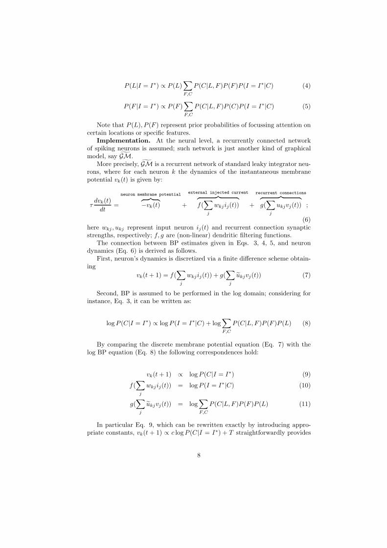
Note that P (L), P (F ) represent prior probabilities of focussing attention oncertain locations or specific features.

Implementation. At the neural level, a recurrently connected networkof spiking neurons is assumed; such network is just another kind of graphicalmodel, say GM.

More precisely, GM is a recurrent network of standard leaky integrator neu-rons, where for each neuron k the dynamics of the instantaneous membranepotential vk(t) is given by:

τdvk(t)

dt=

neuron membrane potential︷ ︸︸ ︷−vk(t) +

external injected current︷ ︸︸ ︷f(

∑

j

wkjij(t)) +

recurrent connections︷ ︸︸ ︷g(

∑

j

ukjvj(t)) ;

(6)here wkj , ukj represent input neuron ij(t) and recurrent connection synapticstrengths, respectively; f, g are (non-linear) dendritic filtering functions.

The connection between BP estimates given in Eqs. 3, 4, 5, and neurondynamics (Eq. 6) is derived as follows.

First, neuron’s dynamics is discretized via a finite difference scheme obtain-ing

vk(t + 1) = f(∑

j

wkjij(t)) + g(∑

j

ukjvj(t)) (7)

Second, BP is assumed to be performed in the log domain; considering forinstance, Eq. 3, it can be written as:

log P (C|I = I∗) ∝ log P (I = I∗|C) + log∑

F,C

P (C|L, F )P (F )P (L) (8)

By comparing the discrete membrane potential equation (Eq. 7) with thelog BP equation (Eq. 8) the following correspondences hold:

vk(t + 1) ∝ log P (C|I = I∗) (9)

f(∑

j

wkjij(t)) = log P (I = I∗|C) (10)

g(∑

j

ukjvj(t)) = log∑

F,C

P (C|L, F )P (F )P (L) (11)

In particular Eq. 9, which can be rewritten exactly by introducing appro-priate constants, vk(t + 1) ∝ c log P (C|I = I∗) + T straightforwardly provides

8

the following relation:

P (C|I = I∗) = ρ exp{vk(t + 1) − T

c} (12)

which defines the spiking probability of a neuron of type C in terms of thedistance between the membrane potential v and the membrane threshold T

Similar relations can be obtained for the other BP equations and F, L vari-ables.

In other terms, Rao’s approach provides a new interpretation of the spikingprobability of cortical neurons in terms of posterior probabilities and is usedto simulate and predict behaviors of neurons within the V4 cortical area underdifferent conditions [Rao, 2005].

From an architectural standpoint, if for instance feature F can take oneamong m values/states {f1, f2, · · · , fm}, then the F node in GM is implemented

by m leaky integrate-and-fire neurons in GM. The same holds for nodes L, C.This shows how the design of GM top-down constrains the design of GM.

4 Discussion

The case study presented above suggests a remarkable conceptual shift withrespect to Marr’s three levels proposal.

In the framework of a Bayesian approach, the computational model M =〈P ({Xk}

Kk=1),GM〉 is fully specified when the graphical model GM has been

defined. Such graphical model indeed is an iconic model of the world W [Giere,2004, Hartmann and Frigg, 2005]; in the case at hand (cfr. Fig. 6) condi-tional dependencies are derived so as to reflect functional dependencies occurringamong brain areas. More precisely, GM is iconic in the sense that the hierarchy(F, L) → C → I reflects the (Parietal,V4) → V2/V1 → Retina hierarchy (cfr.Fig. 6). Thus, computational model M, related to cognitive level activity, isspecified in terms of the underlying neural architecture as illustrated in Fig.6, where GM is conceived as a blueprint for the biological neural architecture.In turn, once GM has been obtained it can be used to top-down constrain thedesign of the artificial neural architecture.

In this respect, the notion of architecture becomes a central tenet in theBayesian approach in defiance of Marr’s methodological effort to provide, in thevein of traditional AI, a careful separation between ”hardware” and ”software”issues.

As a consequence, the algorithmic level rather than encompassing, as forMarr, specific procedures/routines to solve problems stated at the computa-tional level, becomes a general purpose simulation step: it does not depend onwhat is computed (except for structural constraints imposed by GM), and it isusually used for inference and learning (much like learning algorithms in artifi-cial neural nets). Indeed, when BP equations are put into run they provide asimulation (approximate inference), say S of model M.

Two further aspects deserve some comments.

9

First note that Eq. 7 is the discrete form of the differential equation (Eq. 6)that models a leaky integrate-and-fire neuron. Recall that discretization turnsdifferential equations, which relate continuous rates of change over infinitesimalintervals, into difference equations, which relate rates of change over finite, ordiscrete, intervals. The values that these difference equations give can thenbe calculated by a digital computer, in discrete time steps. In other words, aspointed out by Winsberg [2004], ”finite differencing”, namely the transformationof the differential equations into difference equations constitutes a simulation,say S of M, which in the case is the system of differential equations defined ona recurrent network GM of leaky integrate-and-fire neurons.

Second, BP equations also provide the starting point for reduction to whatMarr would call the implementation level. In fact, reduction is achieved bysetting the ”correspondence rules” as in Eq. 9, 10, 11. Interestingly enough,the derivation of model M from M (represented by arrow (1) in Fig. 7 below),is achieved as a sort of inter-theoretic reduction [Nagel, 1961] but where the

bridge principle (see Eq. 12) involves equations used in simulations S and S(cfr. arrow (3) in Fig. 7) rather than a straightforward logical derivation a laNagel [1961] of the laws or principles of the reduced theory (in this case M )

from the laws or principles of the reducing theory M.Eventually, it is clear that different from Marr, the implementation level

itself is a kind of theoretical model M = 〈P ({i, t}Ni=1), GM〉, related in this case

to neural level activity, where GM represents the neural architecture whosedesign is constrained by GM.

The state of affairs that has been so far achieved can be generalized, beyondthe specific example, and summarized at a glance as in Fig. 7

Figure 7: The Bayesian computational model M and the neural model M; Sand S represent software simulations of models M and M, respectively. Arrows(1) and (3) specify ways of reduction from M to M.

The same figure also suggests that in the context we have described, simu-lation S may also be conceived as a coarse grained simulation of the underlyingneural model (arrow (5) in Fig. 7).

10

5 Final remarks

The conceptual shift with respect to Marr’s original proposal is readily apparent.The Bayesian practice reshapes Marr’s original account in a quite differ-

ent story, where levels of explanation become a hierarchy of models (in Rao’s

case M → M interlaced via simulation) and where the notion of architecturebecomes a central one for all levels.

Also, by recalling again Fig. 7, note that process behavior at the neurallevel (differential equations) can in principle be obtained either straightforwardly

(at the same level) by running deterministic finite difference equations (S) orthrough a coarse grained simulation S performed on probabilities: in this per-spective much of the controversial debate on dynamical system hypothesis asopposed to higher level computations becomes an ill-posed question.

Further levels of reduction could be achieved by noting that the firing ratemodel of the neuron described by the dynamical system given by Eq. 6, is asimplified model of neuron (M) [Koch, 1999]. It can be easily related to thestandard cable equation, which in turn can be obtained through mathemat-ical linearization of reaction-diffusion system of partial differential equationscontrolling the spatiotemporal dynamics of calcium ions and bound buffer con-centrations at the chemical level [Koch, 1999].

Thus, in principle, computations can be carried out by using probabilities, orat a lower level using membrane potential as the crucial variable, controlled bythe cable equation, or further at the lower level by taking into account concentra-tion of calcium or or other substances governed by reaction-diffusion equations.As pointed out by Koch (see Koch [1999], p. 279) ”the principal differenceare the relevant spatial and temporal scales dictated by the different physicalparameters, as well as the dynamical range of the [...] sets of parameters”.

Eventually, it is worth noting that at any level l, a model Ml can certainly bealgorithmically simulated, via Sl, but equivalently could undergo a simulationAl, via a physical analog (actually Marr’s original physical realization level).For instance, at the neuron level one could implement the circuit correspondingto the leaky integrate and fire neuron [Koch, 1999]; at a higher level, inferenceon the graphical model could be realized through a special purpose hardwaremessage-passing architecture.

To conclude, the complete picture could be depicted as in Fig 8.In some sense, by taking a Bayesian stance, Marr’s proposal seems more

related to different kinds of model simulation (namely, Al and Sl) at a given levell of explanation, rather than actually involving different levels of explanation.For instance, considering Fig. 8, Marr’s proposal can be accounted for by a singlehorizontal level, whilst the Ml+1 → Ml → Ml−1 hierarchy straightforwardlydenotes the hierarchy of explanations.

11

Figure 8: Hierarchy of models corresponding to hierarchy of explanations.

A The Belief Propagation algorithm for directed

graphs

A general node Xn has messages coming in from parents Par(Xn) and fromchildren Ch(Xn). We can collect all the messages from parents that will be sentthrough Xn to any subsequent children as

µParXn

(Xn) =∑

Par(Xn)

P (Xn|Par(Xn))∏

Xi∈Par(Xn)

µParXi→Xn

(Xi) (13)

Similarly, we can collect all the information coming from the children of nodeXn that can subsequently be passed to any parents of Xn

µChXn

(Xn) =∏

Xi∈Ch(Xn)

µChXi→Xn

(Xn) (14)

The bottom-up messages from children are defined as

µChXi→Xn

(Xn) =∑

Xi

µChXi

(Xi)∑

Xk∈Par(Xi)\Xn

P (Xi|Par(Xi))∏

Xk∈Par(Xi)\Xn

µParXk→Xi

(Xi),

(15)and the top-down messages from parents

µParXk→Xn

(Xk) = µParXk

(Xk)∏

Xi∈Ch(Xk)\Xn

µChXi→Xk

(Xk) (16)

The structure of the above equations is that to pass a message from a nodeX1 to a child node X2 , we need to take into account information from all theparents of X1 and all the children of X1, except X2 . Similarly, to pass a messagefrom node X2 to a parent node X1, we need to gather information from all thechildren of node X2 and all the parents of X2 , except X1.

Such schedule is formalized in the Belief Propagation algorithm:

12

for all evidential nodes Xi do

µParXi

(Xi) = 1 for node Xi in the evidential state, 0 otherwise.

µChXi

(Xi) = 1 for node Xi in the evidential state, 0 otherwise.for all non-evidential nodes Xi with no parents do

µParXi

(Xi) = P (Xi)for all non-evidential nodes Xi with no children do

µChXi

(Xi) = 1for every non-evidential node Xi do

repeat

if Xi has received the µParmessages from all its parents then

calculate µParXi

(Xi).

if Xi has received µCh messages from all its children then

calculate µChXi

(Xi).

if µParXi

(Xi) has been calculated then

for every child Xj of Xi such that Xi has received the µCh messagesfrom all of its other children do

calculate and send the message µParXi→Xj

(Xi)

if µChXi

(Xi) has been calculated then

for every parent Xj of Xi such that Xi has received the µPar mes-sages from all of its other parents do

calculate and send message µChXi→Xj

(Xj)

until all the µCh and µPar messages between any two adjacent nodeshave been calculated

for all non-evidential nodes Xi do

compute the marginal P (Xi|evidence) ≃ µParXi

(Xi) · µChXi

(Xi)

References

N. Chater, J.B. Tenenbaum, and A. Yuille. Probabilistic models of cognition:Conceptual foundations. Trends in Cognitive Sciences, 10(7):287–291, July2006.

R. Cordeschi. The Discovery of the Artificial: Behavior, Mind and MachinesBefore and Beyond Cybernetics. Kluwer Academic Publishers, 2002.

R.N. Giere. How models are used to represent reality. Philosophy of Science,71:742 – 752, 2004.

S. Hartmann and R. Frigg. Scientific Models, volume 2, pages 740–749. Rout-ledge, New York, 2005.

D. Kersten and A. Yuille. Bayesian models of object perception. Current Opin-ion in Neurobiology, 13:150–158, 2003.

D.C. Knill, D. Kersten, and A. Yuille. Introduction: A Bayesian formulation ofvisual perception, pages 1–21. Cambridge University Press, 1996.

13

C. Koch. Biophysics of Computation - Information Processing in Single Neu-rons. Oxford University Press, New York, 1999.

T. S. Lee and D. Mumford. Hierarchical bayesian inference in the visual cortex.J. Opt. Soc. Am. A, 20(7):1434–1448, 2003.

D.J.C. MacKay. Information Theory, inference and Learning Algorithms. Cam-bridge University Press, Cambridge, UK, 2004.

D. Marr. Vision: A Computational Investigation into the Human Representa-tion and Processing of Visual Information. W.H. Freeman, New York, 1982.

M. Mishkin, LG Ungerleider, and KA Macko. Object vision and spatial vision:Two cortical pathways. Trends Neurosci, 6(10):414–417, 1983.

E. Nagel. The Structure of Science. Harcourt, Brace, and World, New York,1961.

M.G. Paulin. Evolution of the cerebellum as a neuronal machine for bayesianstate estimation. J. Neural Eng., 2:219–234, 2005.

R.P.N. Rao. Bayesian inference and attentional modulation in the visual cortex.Neuroreport, 16:1843–1848, 2005.

E. Winsberg. Sanctioning models: The epistemology of simulation. Science inContext, 12(2):275–292, 2004.

14