bayesian modelling of direct and indirect effects of ... · bayesian modelling of direct and...
TRANSCRIPT
Bayesian Modelling
of Direct and Indirect Effects of
Marine Reserves on Fishes
A thesis presented in partial fulfilment
of the requirements for the degree of
Doctor of Philosophy
in
Statistics
at Massey University, Albany, New Zealand.
Adam Nicholas Howard Smith
2016

Copyright is owned by the Author of the thesis. Permission is given for a copy to be downloaded by an individual for the purpose of research and private study only. The thesis may not be reproduced elsewhere without the permission of the Author.

i
Abstract
This thesis reviews and develops modern advanced statistical methodology for
sampling and modelling count data from marine ecological studies, with specific applications
to quantifying potential direct and indirect effects of marine reserves on fishes in north
eastern New Zealand. Counts of snapper (Pagrus auratus: Sparidae) from baited underwater
video surveys from an unbalanced, multi-year, hierarchical sampling programme were
analysed using a Bayesian Generalised Linear Mixed Model (GLMM) approach, which
allowed the integer counts to be explicitly modelled while incorporating multiple fixed and
random effects. Overdispersion was modelled using a zero-inflated negative-binomial error
distribution. A parsimonious method for zero inflation was developed, where the mean of the
count distribution is explicitly linked to the probability of an excess zero. Comparisons of
variance components identified marine reserve status as the greatest source of variation in
counts of snapper above the legal size limit. Relative densities inside reserves were, on
average, 13-times greater than outside reserves.
Small benthic reef fishes inside and outside the same three reserves were surveyed to
evaluate evidence for potential indirect effects of marine reserves via restored populations of
fishery-targeted predators such as snapper. Sites for sampling were obtained randomly from
populations of interest using spatial data and geo-referencing tools in R—a rarely used
approach that is recommended here more generally to improve field-based ecological
surveys. Resultant multispecies count data were analysed with multivariate GLMMs
implemented in the R package MCMCglmm, based on a multivariate Poisson lognormal error
distribution. Posterior distributions for hypothesised effects of interest were calculated
directly for each species. While reserves did not appear to affect densities of small fishes,
reserve-habitat interactions indicated that some endemic species of triplefin (Tripterygiidae)
had different associations with small-scale habitat gradients inside vs outside reserves. These

ii
patterns were consistent with a behavioural risk effect, where small fishes may be more
strongly attracted to refuge habitats to avoid predators inside vs outside reserves.
The approaches developed and implemented in this thesis respond to some of the
major current statistical and logistic challenges inherent in the analysis of counts of
organisms. This work provides useful exemplar pathways for rigorous study design,
modelling and inference in ecological systems.

iii
Preface
I acknowledge the generous financial support of the Department of Conservation
(Project Inv 4238), and Massey University’s Institute for Natural and Mathematical Sciences
(INMS) for providing a scholarship and, ultimately, a job. There are many people at Massey I
wish to thank, including various office mates (Insha Ullah, Olly Hannaford, Rina Parry,
Helen Smith, and Ting Dong), our wonderful administrative staff (Annette Warbrooke, Freda
Mickisch, Lyn Shave, Anil Malhotra, Colleen Keelty (Van Es), and Vesna Davidovic-
Alexander), and my INMS colleagues, particularly in the statistics and ecology groups, and
my next-door-office neighbours, David Aguirre and Libby Liggins. Thanks also go to Assoc.
Prof. Ann Dupuis for her advice and support through this process.
I could not have wished for a better primary supervisor than Professor Marti
Anderson. Thank you, Marti, for always believing in me, despite often being confronted with
compelling reasons not to. There were moments, in the latter stages, when you knew just the
right thing to say to inspire me to grab this thing by the appendix and wrestle it into
submission. You have given me so much and taught me so much about so many things but,
foremost, thank you for being, in your words, my sternest critic and ultimately my biggest
fan. Thanks also to my co-supervisor Russell Millar for keeping me on the methodological
straight and narrow. Thank you to my late-coming co-supervisor, Matthew Pawley, for many
many reasons, but especially for the daily laughs and near-annual overseas adventures. Rather
ironically, you’ve helped me keep my sanity through all this. I look forward to working with
you in future, especially now that I am technically no longer your subordinate.
Many people spent long hours underwater counting fish for this PhD, including Oliver
Hannaford, Marti Anderson, Steve Hathaway, Severine Dewas, Paul Caiger, Clinton Duffy,
Charles Bedford, Kirstie Knowles, Nick Macrae, Sietse Bouma, Dave Culliford, Caroline
Williams, and Alice Morrison. Particular thanks go to Clinton Duffy of the Department of

iv
Conservation for skippering the RV Tuatini, and commenting on various manuscript drafts.
Also, thank you to Steve Hathaway for bringing me fame by putting me on TV and in a book,
and having the audacity to dub me a “guru”.
More broadly now, I wish to thank the people who inspired me to pursue a
professional career in statistical and ecological research, and supporting me when it began in
2002, namely Jennifer Brown (University of Canterbury), Ian Westbrooke, and Ian West. I
also thank Clinton Duffy (Department of Conservation) for showing me the water from the
trees and inspiring my conversion to the study of things marine (you’re next, mate). A warm
thank you goes to my father, Dr Murray Smith, for passing to me a small fraction of his
extraordinary talent for statistics, and for encouraging me to take it on, along with other good
advice when I needed it. Being able to work with you at NIWA has been a highlight of my
career.
On a more personal note, I now turn to my little family. Being part of this family is
the greatest privilege of my life. To my exquisite wife, Heidi, I offer you an ocean of
gratitude for your unwavering support and patience. You are amazing and I could not have
done this without you. Finally, to my beloved children, Finley and Anna. I am so proud and
honoured to be your father. I cannot say that you made this endeavour any easier, but you and
your mother make it and everything else worthwhile. My masters thesis was dedicated to
Heidi, for it was during my masters that she agreed to marry me. You two graced our lives
during this PhD, and I wholeheartedly dedicate it to you.

v
Me, bombastically gesticulating to Marti’s bemusement.
Poor Knights Islands. (Photo credit: Steve Hathaway).

vi
Table of contents
Chapter 1. General introduction ............................................................................................ 1
1.1 Direct and indirect effects of marine reserves .................................................. 1
1.2 Challenges in evaluating the effects of marine reserves .................................. 3
1.3 Aims ................................................................................................................. 7
1.4 Overview of chapters ....................................................................................... 9
Chapter 2. A review of Bayesian generalised linear mixed models for ecological studies 13
2.1 Introduction .................................................................................................... 13
2.2 Bayesian statistics—the basics ....................................................................... 15
2.3 Example: an observational study of a marine reserve .................................... 20
2.4 Generalised linear models .............................................................................. 22
2.5 Analysis of variance and mixed-effects models ............................................. 29
2.6 Model fitting ................................................................................................... 39
2.7 Model evaluation and selection ...................................................................... 43
2.8 Concluding remarks ....................................................................................... 52
Chapter 3. Sources of zeros in ecological abundance data (Prologue to the study of
snapper—Chapters 4 and 5) .............................................................................. 54
3.1 Introduction .................................................................................................... 54
3.2 Zero counts in ecology ................................................................................... 54
3.3 Excess zeros and the occupancy-abundance relationship .............................. 58
3.4 Zeros in counts of snapper from baited underwater video surveys ................ 62
3.5 Concluding remarks ....................................................................................... 70
Chapter 4. Incorporating the intraspecific occupancy-abundance relationship into zero-
inflated models .................................................................................................. 72
4.1 Abstract .......................................................................................................... 72
4.2 Introduction .................................................................................................... 73

vii
4.3 The linked zero inflation model ..................................................................... 76
4.4 Example .......................................................................................................... 77
4.5 Discussion ...................................................................................................... 83
4.6 Conclusion ...................................................................................................... 87
4.7 Acknowledgements ........................................................................................ 87
Chapter 5. Effects of marine reserves in the context of spatial and temporal variation: an
analysis using Bayesian zero-inflated mixed models ........................................ 89
5.1 Abstract .......................................................................................................... 89
5.2 Introduction .................................................................................................... 90
5.3 Materials and methods ................................................................................... 92
5.4 Results .......................................................................................................... 101
5.5 Discussion .................................................................................................... 108
5.6 Acknowledgements ...................................................................................... 115
Chapter 6. Marine reserves indirectly affect fine-scale habitat associations, but not density,
of small benthic fishes ..................................................................................... 117
6.1 Abstract ........................................................................................................ 117
6.2 Introduction .................................................................................................. 118
6.3 Methods ........................................................................................................ 122
6.4 Results .......................................................................................................... 128
6.5 Discussion .................................................................................................... 139
6.6 Acknowledgements ...................................................................................... 143
Chapter 7. Could ecologists be more random? ................................................................. 144
7.1 Abstract ........................................................................................................ 144
7.2 Main text ...................................................................................................... 144
Chapter 8. General discussion ........................................................................................... 154
8.1 Ecological effects of marine reserves........................................................... 154
8.2 Statistical methodology ................................................................................ 159
8.3 Summary ...................................................................................................... 166

viii
Literature cited 168
Appendix A Supplementary Material for Chapter 4 .............................................................. 198
A.1 Formal description of linked zero-inflated negative binomial model .......... 198
A.2 Table of summary statistics for estimated parameters ................................. 201
A.3 Potential relationships λ and π under linked zero-inflation .......................... 202
A.4 R and OpenBUGS code and data ................................................................. 203
A.5 Convergence diagnostics .............................................................................. 205
A.6 Posterior predictive checks........................................................................... 208
A.7 Sensitivity Analysis ...................................................................................... 212
Appendix B Supplementary Material for Chapter 5 .............................................................. 219
Appendix C Supplementary Material for Chapter 6 .............................................................. 220
Appendix D Supplementary Material for Chapter 7 .............................................................. 221
D.1 Table of useful spatial functions in R........................................................... 221
D.2 Code for implementing random sampling designs ....................................... 222
Appendix E Contribution to co-authored chapters ................................................................ 223

ix
List of tables
Table 4-1. A comparison of a selection of candidate models for estimating the counts of
legally sized snapper from a marine reserve monitoring program. For all models shown here,
the base distribution for the counts was the negative binomial. Four classes of zero-inflated
models were used, as indicated by the model numbers: (1) no zero inflation, (2) constant zero
inflation, (3) a separate linear predictor for zero inflation, and (4) zero inflation linked to the
mean of the count process. In the case of model 3, submodels 3.1–3.4 contain increasing
numbers of parameters in the separate linear predictor for zero-inflation, as indicated. The
predictor variables are denoted as follows: R = reserve status; S = season; A = area; Y = year.
Models were compared using the Deviance Information Criterion (DIC) and its summands,
the expected deviance (𝑫) and the effective number of parameters (𝒑𝑫). The actual number
of stochastic parameters (𝒑) is also provided. The mean of the posterior predictive
distributions for the total number of zeros (Total 𝒏𝟎) and the total count (Total 𝒕) is presented.
These may be compared with the same values from the observed data, namely 191 and 660,
respectively. Finally, estimates of the mean absolute error for each of 𝒏𝟎 and 𝒕, pooled at the
level of replicate bins, provide the “mean bin misclassification rate” (Bin 𝝐𝒏𝟎) and the “mean
bin absolute deviation” (Bin 𝝐𝒕). For these measures, smaller values indicate more accurate
predictions. (See Appendices A.1 and A.6 for further details of the model and posterior
predictive checks.) ................................................................................................................... 81
Table 5-1. Details regarding the age and size of each of the three marine reserves examined
in this study. ............................................................................................................................. 93
Table 5-2. The number of baited underwater video (BUV) sampling units obtained in each
year, season and location. Samples within each survey were allocated to reserve and non-
reserve areas equally in most cases. ......................................................................................... 93
Table 5-3. Sources of variation for the full ANOVA model, based all factors in the study
design. The terms that were not included as candidates for model selection, based on
preliminary heuristics, are indicated with an asterisk. The abbreviation for each term, as
shown, was used to indicate the model parameters associated with that term in the GLMs,
given in Equations (5-3) to (5-5) in the text. Terms that were chosen to be included in the
final models of relative densities of legal or sublegal snapper, obtained using model selection
on the basis of the DIC, are also provided. .............................................................................. 97
Table 5-4. Point estimates (mean of the posterior distribution, represented by the set of
values given by MCMC) and 95% credible intervals (0.025 and 0.975 quantiles of the
posterior distribution) of the mean relative densities for either sublegal or legal snapper in
reserve and non-reserve areas at each of three locations. Reserve and non-reserve densities
for sublegal snapper were pooled because there was no reserve effect in the model. Estimates
of the ratio of reserve to non-reserve densities are also provided for legal snapper as an index
of the ‘reserve effect’. The point estimates for the ratios were obtained by first calculating the
ratios for each MCMC iteration, taking the natural log of the ratios, calculating the mean, and
then back-transforming. ......................................................................................................... 102

x
Table 5-5. Point estimates and 95% credible intervals (as described in the legend for Table
5-4) of the mean relative densities for either legal or sublegal snapper in each of two seasons
at each of three locations. Estimates for ratios of seasonal effects were obtained as described
for reserve effects in the caption for Table 5-4. ..................................................................... 105
Table 6-1. The habitat features (and definitions) for which presence or absence was recorded
in each quadrat. Also provided here are the loadings (standardised coefficients) of each
habitat feature for each of the first three principal component axes from a PCA of 12 habitat
variables. Loadings that exceed 0.4 are shown in bold.......................................................... 124
Table 6-2. Taxa detected in the surveys, including the number of individuals of each taxon
observed in the whole dataset. Most taxa were consistently identified to species, including all
triplefins (TF). Moridae consisted mostly of the species Pseudophycis breviuscula and
Lotella rhacina. Gobiesocidae were Dellichthys morelandi or Gastrocyathus gracilis.
Acanthoclinus spp. were most likely the species A. rua, A. marilynae, or A. littoreus. The nine
most abundant species are indicated by an asterisk (*) and these were modelled individually.
................................................................................................................................................ 131
Table 6-3. Permutational multivariate analysis of variance (PERMANOVA) tests for the
effects of variables on the structure of assemblages of benthic reef fish, based on Bray-Curtis
distances of the transect-level abundance of all species. There were 635 residual df, and tests
were based on Type III partial sums of squares and 999 permutations. ................................ 132
Table 7-1. Systematic review of methods used to choose spatial sampling units in recent
ecological studies. We conducted a census of articles which resulted from a search on 7 July
2013 in Biological Abstracts. Search parameters were Year=2013, Topic=((abundan* OR
densit*)), Major Concepts=(ECOLOGY), and Source Titles=(Diversity and Distributions,
Ecological Applications, Ecology, Ecology Letters, Journal of Applied Ecology, Journal of
Animal Ecology, Journal of Ecology, Oecologia, or Oikos). We only included studies that
involved observations or experiments in the field, using spatially-replicated sampling units.
Field experiments from a single block which was then divided into subplots were excluded.
The allocation of treatments to units in experimental studies was not considered—we were
only interested in the method used to choose the spatial locations of units. A total of 99 out of
215 articles met our criteria for review. ................................................................................. 147
Table A-1. Prior distributions for stochastic parameters. ..................................................... 199
Table A-2. Summary statistics of the posterior distributions of estimated parameters,
including the mean, standard deviation (SD), median, and 95% credible intervals (CI). ..... 201
Table A-3. Summary of posterior predictive checks, by way of comparison of five summary
test quantities calculated from the data (𝑻(𝒚)) with the posterior predictive distributions of
the same test quantities, calculating from 5,000 replicate datasets simulated from the
model (𝑻(𝒚𝐫𝐞𝐩)). Q 0.05 and Q 0.95 give the 90% credible intervals for the posterior
predictive distributions........................................................................................................... 210

xi
Table A-4. List of models that were compared with the base model (1–lZNB) in a sensitivity
analysis, with a coded description of their error structure as follows. Linked, Separate, and
Constant zero inflation are indicated by LZI, SZI, and CZI, respectively (see Chapter 4 for
definitions). For linked zero inflated model, the zero-inflation probability 𝝅 was fitted as a
function of the mean of the count distribution 𝝀, specifically, f(𝝅) = 𝜸𝟎 + 𝜸𝟏 log(𝝀), with f
being the logit or the cloglog function, as indicated. Distributions used to model count values
were Poisson (P), negative binomial (NB), or Poisson lognormal (PLN). The way in which
each model differed from the base model is also explicitly described. Prior distributions used
in the base model (for parameters whose priors were modified in other models herein) were
as follows: 𝜷𝟎, 𝜷𝑺, 𝜷𝑹, 𝜸𝟎, 𝜸𝟏 ~ N(0, 100); 𝝈𝑨, 𝝈𝒀 ~ half-Cauchy(0,1); 𝜹 ~ Gamma(10-4, 10-
4). An estimate and precision of the log reserve effect (shown as mean 𝐋𝐑𝐄 and standard
deviation 𝒔𝐋𝐑𝐄 of the posterior distribution) is given for each model. .................................. 214

xii
List of figures
Figure 2-1. Three alternative ways to graphically display an ANOVA design. The two
dendrographs are a popular way of depicting an ANOVA design, but are not ideal for designs
with both crossed and nested factors. The top dendrograph demonstrates that factors M and L
are crossed by linking each level of one to each of the other, but it is then implied that there
are only nine Areas in total, which is incorrect. Alternatively, the lower dendrograph shows
that each level of L is replicated and achieves the correct number of Areas, but this visually
implies that L is nested in M, as opposed to being crossed. The table logically displays the
structure of the design while clearly indicating where factors are crossed or nested. Each cell
represents a mean that is estimated. ......................................................................................... 21
Figure 2-2. An illustration of overdispersed counts in a spatial context, by way of contagion
and excess zeros. The points in panel A are randomly distributed without contagion or excess
zeros; thus, counts take from the underlying squares would not be overdispersed (the variance
would equal the mean). Note that panel C contains a greater number of empty cells than panel
A, illustrating that more zeros can arise through contagion alone without any explicit process
that produces excess zeros (Warton 2005). .............................................................................. 25
Figure 2-3. Comparison of estimates of group means for treating the grouping factor as (a)
fixed and (b) random, made by two models of the same dataset, plotted here on the same
scale. The coloured circles at the bottom level represent the observed data, comprising three
observations from 8 groups, which are connected by dotted lines to the estimates of their
corresponding group means (coloured squares). For the fixed effect, there is no distribution
fitted to the group means—they are simply estimated as the mean of the comprising values.
For the random effect, a normal distribution was fitted with an estimated variance
component, represented in grey. This results in more conservative estimates of the group
means— they are shrunk toward the global mean. For both models, the errors from the group
means were assumed to be normally distributed with an estimated error variance (as
represented coloured distributions). ......................................................................................... 34
Figure 2-4. Density of the Cauchy distribution with scale-parameter values of 1–3 (x-axis
truncated at 8). ......................................................................................................................... 35
Figure 3-1. A schematic diagram of a spatial intraspecific occupancy-abundance relationship
(OAR). The locations of individuals in the study domain are shown in A. The shade of the
small cells in B indicates the relative abundance of individuals per cell; white squares
indicate non-occupancy. The OAR is illustrated in C at the spatial scale of the larger squares
in B (each comprised of 6 × 6 cells); the number of occupied cells is positively related to the
mean abundance per cell (figure reproduced from Borregaard and Rahbek 2010, with
permission from Univ. of Chicago Press). ............................................................................... 59

xiii
Figure 3-2. The baited underwater video apparatus as used in the study of snapper (from
Willis and Babcock 2000). ....................................................................................................... 64
Figure 3-3. The occupancy-abundance relationship for legal (A) and sublegal (B) snapper,
represented by the log conditional mean of the counts (𝝀𝒊) plotted against the logit probability
of excess zero (𝝅𝒊) estimated for each combination of area-by-year. The plotted numbers
indicate the areas, and colours indicate inside (red) vs outside (black) marine reserves. These
estimates came from zero-inflated models in which 𝝅𝒊 and 𝝀𝒊 were fitted using separate linear
predictors of the factors. .......................................................................................................... 68
Figure 4-1. The relationship between the conditional mean count (λ) of snapper (per baited
underwater video deployment) and the probability of an excess zero (π) for legally sized
snapper from a marine reserve monitoring program. This relationship was estimated using a
Bayesian zero-inflated model (Appendix A.1) where π and λ were linked explicitly as logit(π)
= γ0 + γ1log(λ). The black line shows this function using point estimates for the parameters
of γ0 = 0.34 and γ1 = –1.60. The grey lines show this function using the paired values of these
parameters under MCMC within their joint 95% credible bounds. ......................................... 82
Figure 5-1. A map showing the locations of three marine reserves in north-eastern New
Zealand (upper left panel). Also shown are the individual numbered areas (fine lines and
numbers), and marine reserves (bold lines) at each location, as indicated. Note that the
borders of Tāwharanui Marine Reserve were moved slightly in September 2011 and are now
different to those shown here. .................................................................................................. 94
Figure 5-2. A variance components plot (Gelman 2005) showing the variation associated
with each term in the chosen models, expressed as the estimate of the standard deviation σ
among levels, for predicting the relative density of legal or sublegal snapper. For the latter,
separate linear predictors were used to model the probability of an excess zero (π) and the
conditional mean of the counts (λ), so a separate panel is used for each. Point estimates
(means of posterior distributions) are represented by vertical lines, with 50% and 95%
credible intervals for the means as thick and thin horizontal lines, respectively. .................. 103
Figure 5-3. Fine-scale spatial patterns in the estimated mean relative density of sublegal
(triangles) and legal (circles) snapper, in areas within three locations. Open and closed
symbols represent the point estimates (means of posterior distributions) for spring and
autumn, respectively. Error bars are 95% credible intervals for the means. ......................... 106
Figure 5-4. Inter-annual and season patterns in the estimated mean relative density of
sublegal (triangles) and legal (circles) snapper at three locations. Open and closed symbols
represent the point estimates (means of posterior distributions) for spring and autumn,
respectively. Error bars are 95% credible intervals for the means. For legal snapper, estimates
for within the reserves only are shown, because too few snapper were observed outside the
reserves to show any interpretable patterns. Note that the scale of the y-axes varies differ for
sublegal (left) and legal (right) panels. .................................................................................. 107

xiv
Figure 6-1. Predicted interactive effects of marine reserves (where a generalist predator is
more abundant) and habitat complexity (where more complex habitat provides greater refuge
from predation) on the densities of prey fish, under two different mechanisms. The two lines
represent prey densities inside (in orange) and outside (in blue) marine reserves. In (a), the
primary mechanism causing the interaction is predation, particularly in areas of low-
complexity habitat. In this case, a main effect of reserve status is expected, where overall
mean densities are lower inside reserves. In (b), the primary mechanism is a risk effect where
prey fish, due to the abundance of predators, prefer more complex habitat in order to avoid
predation. Here, no main effect of reserve status is expected and the average heights of the
two lines are equivalent. ........................................................................................................ 121
Figure 6-2. Map of the three locations and 35 sites. ............................................................ 123
Figure 6-3. Boxplots showing the distribution of values of depth and the three PCA axes for
habitat for reserve and non-reserve transects at each location. ............................................. 129
Figure 6-4. Non-metric multidimensional scaling (MDS) plots of (a) the Site-by-Year
centroids and (b) Location-by-Reserve-by-Year centroids, in Bray-Curtis space, shown by
Location and Reserve status (R = reserve, NR = non-reserve). The 2-d stress for the MDS
analyses were 0.13 (a) and 0.07 (b). ...................................................................................... 133
Figure 6-5. Estimated mean densities per 5-m2 transect for each combination of Location,
Reserve status, and Year, with 95% credible intervals, for (a) species richness, (b) total
number of fish, and (c–k) each of the nine most-common species. Estimates are for a
standardised median habitat at a depth of 10 m. In some cases, the y-axes for (e–k) are shown
on a square-root scale for clarity. ........................................................................................... 134
Figure 6-6. Estimated main effects of marine reserves, shown here as means and 95%
credible intervals of the log ratios of Reserve vs Non-reserve means. They are shown for the
overall study (i.e. calculated from reserve and non-reserve means that were averaged, or
‘marginalised’, across all Location-Year combinations), for each Location (averaged across
Years), and for each Year (averaged across Locations). Filled circles indicate that the 95%
credible interval does not contain zero, suggesting a non-zero difference associated with
Reserve status. These estimates are standardised for habitat and depth using Bayesian
hierarchical models. ............................................................................................................... 135
Figure 6-7. Coefficients associated with the habitat axes, represented by the means and 95%
CIs of the posterior distributions of coefficient values, estimated for the overall study and for
each Location. Symbols for which the CI does not contain zero are filled, suggesting
evidence for a non-zero habitat association. .......................................................................... 136
Figure 6-8. Reserve-Habitat interactions, represented by the means and 95% CIs of the
posterior distributions of the differences between the habitat coefficients inside vs outside
reserves, estimated for the overall study and for each Location. Symbols for differences for

xv
which the CI does not contain zero are filled, representing evidence for a non-zero
interaction. ............................................................................................................................. 137
Figure 6-9. Exploration of Reserve-Habitat interactions, represented here as mean densities
across the range of values of the habitat variables, estimated separately for inside and outside
reserves, for the overall study and for each Location. Hab1 represents a gradient of increasing
complexity, and Hab2 represents a gradient of sandy broken-up reef to solid reef with closed
Ecklonia canopy. The y-axes are shown on a square-root scale for clarity. .......................... 138
Figure 7-1. Three simple sampling designs for selecting 20 sites (pluses) from within
Tāwharanui Marine Reserve (orange) off Tāwharanui Peninsula (grey), near Auckland, New
Zealand. All three designs were implemented in R by applying the function spsample to a
polygon object Strata, in which the reserve is represented by four strata equally spaced along
the seaward border. The designs shown are (1) Simple Random Sample—points selected
randomly through the entire reserve [spsample(Strata, n=20, type="random")]; (2)
Systematic Sample—points selected on a regular grid [spsample(Strata, n=20,
type="regular")]; (3) Stratified Random Sample—five points selected from each of the
four strata [lapply(Strata@polygons, spsample, n=5, type="random")]. Note
that, in the latter case, five sites were taken from within each of the four strata for simplicity.
In practice, it may be more efficient to allocate samples proportional to the stratum areas,
which are straightforward to calculate in R (Table 2). These designs were all implemented
using only freely available data. See Appendix D for further details, including full R code and
data. ........................................................................................................................................ 151
Figure 7-2. A more complex sampling design for Tāwharanui Marine Reserve (see Figure
7-1) targeting specific habitat and depth in four strata. The sampling frame and population of
interest here was rocky reef habitat at depths of five meters. Panel A shows three spatial
objects, representing the marine reserve (Strata, orange polygon), rocky reef (Reef, blue
polygon) and a 5-m contour (Contour, black line). Three steps were taken to obtain the
sample, as follows: 1. Convert the contour into regular points [Pts <-
spsample(Contour, n=1000, type="regular")]. Note that, for clarity, only 100
points are shown in Panel B. 2. The points that overlie reef (black dots, panel B) are selected
as candidate points while those that do not (white dots) are discarded [PtsR <-
Pts[!is.na(over(Pts, Reef)),]]. 3. Randomly select five points from the candidates
in each stratum (pluses in panel C) [PtsRS <- tapply(PtsR, over(PtsR,
Strata)$Name, sample, size=5)]. See Appendix D for further details, including full R
code and data.......................................................................................................................... 152
Figure A-1. Potential relationships between the mean of the count distribution (λ) and the
probability of an excess zero (π) under the general form of the linked model, logit(π) = γ0 +
γ1log(λ). The four lines in each panel have a different value of the intercept (γ0) and a
common slope (γ1), as indicated. A large negative slope (γ1 = –10) permits very fast transition
from complete zero-inflation to no zero-inflation (A). This may be useful if low numbers are
uncommon, so that zeros dominate below a particular threshold value of λ. Smaller negative

xvi
values of the slope can give a range of curves for decreasing zero-inflation with increasing
abundance (B, C, D). For γ1 = 0 (E), the relationship disappears and the model reduces to a
constant value of π, as in model 2. While presumably unusual in nature, positive relationships
between excess zeros and mean abundance can be generated (F). ........................................ 202
Figure A-2. Density histograms of posterior distributions of key model parameters, including
the log of the reserve effect (“log.res.effect”). Mean and median values are shown as green
and red vertical lines, respectively. ........................................................................................ 206
Figure A-3. Trace plots of the three MCMC chains, each shown in a different colour, of key
model parameters, including the log of the reserve effect (“log.res.effect”). ........................ 206
Figure A-4. Convergence diagnostic plots for model parameters (produced by the function
plot.bugs() from the R2OpenBUGS package for R). The two plots on the left show the 80%
credible intervals for each of the three chains in a different colour, and the Brooks-Gelman-
Rubin convergence diagnostic 𝒓 (= “R-hat”). The plots on the right show overall medians and
80% credible intervals for the parameters and the deviance. Parameter “r” here is the
dispersion parameter 𝜹. .......................................................................................................... 207
Figure A-5. Comparison of sorted data values between the observed data 𝒚 (x-axis) and
5,000 replicate datasets 𝒚𝐫𝐞𝐩 simulated under the fitted model (y-axis). The points represent
mean values across the 𝒚𝐫𝐞𝐩 for each corresponding ranked value of 𝒚. The grey polygon
represents the 5% and 95% percentiles of values for 𝒚𝐫𝐞𝐩 at the corresponding rank. E.g., the
highest value in the observed data was 25, whereas the highest values in the 𝒚𝐫𝐞𝐩 datasets
was on average 22 and typically ranged from 15 to 33. ........................................................ 209
Figure A-6. Sensitivity analysis in which the estimated log of the reserve effect from the base
model (linked zero-inflated negative binomial, lZINB) is compared with a range of
alternative models. Values shown represent means, and 2.5% and 97.5% quantiles, of the
posterior distributions. ........................................................................................................... 216
Figure A-7. Sensitivity analysis in which the estimated means of counts (i.e., relative density
of snapper) from non-reserve vs reserve areas from the base model (linked zero-inflated
negative binomial, lZINB) are compared with a selection of alternative models. Values
shown represent means, and 2.5% and 97.5% quantiles, of the posterior distributions. ....... 216

1
Chapter 1. General introduction
1.1 Direct and indirect effects of marine reserves
Both the world population of humans and the per-capita consumption of fish
increased considerably in the second half of the 20th century (FAO 2014). Historically, the
majority of fisheries catch has been taken from coastal areas of the northern hemisphere
(Pauly et al. 2005), and consisted primarily of large apex predators (Pauly et al. 1998). Now,
many fisheries are at or near the point of collapse, with the biomass of some populations
reduced by up to 90% (Myers et al. 1997, 2007, MacKenzie et al. 2009). The majority of fish
consumed by humans is still sourced from wild populations. a growing proportion is
produced by aquaculture, though the feed for farmed fish is largely sourced from wild
populations of smaller fishes (Naylor et al. 2000). To meet demand, fisheries have
increasingly expanded into deeper water and more remote areas of ocean, particularly the
southern hemisphere, and to species that occupy lower trophic levels (Pauly et al. 2005).
Unsurprisingly, recent decades have seen a growing concern about the extent of overfishing
and the ecological impacts of removing top predators from marine ecosystems (e.g. Pauly et
al. 2005, Frank et al. 2005, Worm et al. 2006, Heithaus et al. 2008, Pikitch 2012).
Marine protected areas are a spatial management tool used as part of the effort to
reverse and mitigate the impacts of fishing. In particular, no-take marine reserves, defined by
Lubchenco et al. (2003) as “areas of the ocean completely protected from all extractive and
destructive activities”, have been established in many coastal regions world-wide over the
past few decades. Empirical studies have clearly demonstrated that, in most cases, species
targeted by fisheries show substantial recovery inside marine reserves, with respect to
density, biomass, and the size-age structure of populations. For example, one meta-analysis
estimated that, on average, counts of fish were 3.7 (95% confidence interval: 1.57–5.13)
times greater inside marine reserves than at comparable nearby areas or the same areas prior

2
to the marine reserve being established (Mosquera et al. 2000, but see also Côté et al. 2001,
Molloy et al. 2009, Lester et al. 2009). The direction and magnitude of responses to marine
reserves vary substantially among species and reserves but, in general, the greatest positive
responses occur in intensively fished, larger-bodied, predatory species (Molloy et al. 2009,
Claudet et al. 2010, Guidetti et al. 2014) and larger, older, isolated, and well-enforced
reserves (Edgar et al. 2014).
While ecosystems inside marine reserves remain subject to broad-scale impacts such
as pollution and climate change, they are (obstensibly) exempted from fishing—the greatest
direct human impact on marine ecosystems (Jackson et al. 2001). Thus, ecosystems in
successful marine reserves may represent more ‘natural’ states, resembling, to some extent,
those that existed prior to intensive fishing. Little empirical study of subtidal ecosystems
occurred prior to fishing, so direct, systematic, historical comparisons are largely unavailable.
However, very remote areas, where very little fishing has taken place, do indeed resemble
marine reserves in that they have very large biomasses of large, apex predators (relative to
those of lower trophic levels) (DeMartini et al. 2008). Though not a replacement for sound
fisheries management, the potential of marine reserves to help safeguard species and
ecosystems against fishing is clear (Allison et al. 1998, Roberts et al. 2005, Mora and Sale
2011).
Marine reserves are considered tools for conserving not only fished species, but
biodiversity more broadly (e.g. Agardy 1994). In ecosystems where fishing involves
significant damage to habitats or bycatch, such as trawling on soft sediments (Collie et al.
2000), marine reserves can directly benefit species that are not the target of fishing (Game et
al. 2009). Otherwise, indirect effects of reserves on any non-targeted species could
potentially occur through some ecological relationship (or series of relationships) with a
targeted species, such as direct predation, mutualism, or other interaction (Pinnegar et al.

3
2000). Perhaps the most dramatic example of an indirect effect is the restoration of trophic
cascades in some temperate reef ecosystems, where enhanced populations of predators in
reserves reduced the density of herbivorous sea urchins to the point where forests of
macroalgae recovered and replaced less-productive and less-biodiverse ‘urchin-barrens’
habitat (e.g. Sala et al. 1998, Steneck 1998, Edgar and Barrett 1999, Behrens and Lafferty
2004, Micheli et al. 2005, Leleu et al. 2012). This phase-shift in community structure has
occurred in several temperate reef ecosystems worldwide, including New Zealand (Babcock
et al. 1999, Shears and Babcock 2003), with the identities of the species involved in each of
the three trophic levels (i.e. predator, herbivore, and primary producer) varying among
geographic locations (Ling et al. 2015). Yet, the effect is far from ubiquitous, and can vary
substantially even within a single region (Shears et al. 2008).
Indeed, the presence and magnitude of direct effects and, to a greater extent, indirect
effects of marine reserves generally depend on the ecological and environmental context
(Shears et al. 2008, Salomon et al. 2010). For marine reserves to be used effectively as a tool
for the management of fisheries or conservation, it is imperative that their ecological effects
are understood and, to some extent, able to be predicted. This requires empirical studies that
monitor changes in biological communities in existing reserves across a range of
environmental contexts. Despite a large and growing body of research, there remain
significant gaps in our understanding of the effects of marine reserves for many taxa, and few
general patterns have emerged. The enhancement of our knowledge of direct and indirect
effects of marine reserves motivated the choice of subject-matter for this thesis.
1.2 Challenges in evaluating the effects of marine reserves
Researchers investigating the effects of marine reserves face many methodological
challenges. Ideally, the effects of reserves would be evaluated with monitoring data collected
from inside reserves and a number of comparable control sites, both before and after reserves

4
were established. For many marine reserves, monitoring data from before establishment is not
available, so evaluations are largely based solely on comparisons of inside vs outside
reserves. Strictly speaking, for inferences to generalise to potential future reserves, a number
of replicate reserves would be randomly assigned to the spatial domain of the study. This has
rarely been the case; the placement of marine reserves is generally decided by government
based on socio-political processes that might have considered a range of biological (e.g.
biodiversity value or ecological representativeness) and socio-economic (e.g. willingness of
the local community, disruption to existing fishing areas) factors. Moreover, many studies
have included only a single reserve and/or only a single time period, essentially making them
case studies and limiting their utility as a basis for making preditions for future reserves
(Willis et al. 2003b).
While scientists have little control over the number and placement of replicate
reserves, they do control the replication and placement of sampling sites at smaller scales.
Yet, like in many areas of ecology, many studies of reserves are poorly designed, with
insufficient replication and employing non-random (haphazard) approaches to selecting study
sites, further compromising the strength and validity of inferences. Any effects of reserves
occur within a context of considerable spatial and temporal variation at a variety of scales
(García-Charton and Ruzafa 1999), generating the need for well-designed, long-term
hierarchical sampling regimes with replication spanning important scales of variation (e.g.,
seasons, years, locations, sites, etc.) to obtain rigorous estimates of any effects of
management (Hurlbert 1984, Andrew and Mapstone 1987). The extent to which the
communities vary in time and space at different scales is interesting in itself, and quantifying
such variation provides a useful basis for comparison with any observed reserve effects.
Moreover, biological communities are related to environmental characteristics and habitat
structure at a wide range of spatial scales, so any potential differences in abiotic factors inside

5
vs outside reserves may confound evaluations of reserve effects. Poorly designed and
inadequately replicated studies that do not control for potential differences in environment
and habitat in some way, through explicity study design or statistical modelling, may
incorrectly attribute spatial differences in biological communities to a reserve effect when
they may, in fact, be due, at least in part, to other factors. While the need to compare the
magnitude of reserve effects with other sources of variation and to account for any potential
differences in environment and habitat has been articulated (García-Charton and Ruzafa
1999, García-Charton et al. 2004), appropriate statistical methods for doing so have not been
explicitly specified in this context.
Even well-designed ecological studies can pose significant challenges when it comes
to statistical analysis, as complex models are often required to accurately quantify effects of
interest. Replication of sampling units at multiple spatial or temporal scales, as required to
avoid pseudoreplication (Hurlbert 1984), gives rise to complex hierarchical designs that are
best analysed with mixed-effects models, often with multiple fixed and random effects, and
interactions. It is also common for designs to be unbalanced in terms of the number of data
points within different combinations of factors, due to data being collected opportunistically
or sampling events being weather-dependent.
Response variables for ecological studies are often some measure of the density of
organisms, usually recorded as counts taken from a standardised unit such as a quadrat or
transect of a fixed size. A standard approach to analysing count data is to use a Poisson
distribution to model the errors from fitted means. While the Poisson distribution is
charmingly simple—having only a single parameter giving both the mean and the variance—
it requires individuals to occur independently of one another. Few organisms have such
disregard for one another (Taylor 1961). Hence, counts of organisms often fail to conform to
a Poisson distribution, having greater variance and an excessive number of zeros than would

6
be expected given the mean, a condition known generally as overdispersion (Cole 1946). We
are often warned that failure to account for overdispersion, where it occurs, can result in
underestimation of the sampling error associated with parameters and result in inaccurate
conclusions (e.g. Potts and Elith 2006).
Some studies include multiple species of interest, yielding response variables of
multivariate counts. While statistical methods for modelling multivariate continuous response
variables are well developed, methods for modelling multivariate, discrete data, such as
counts, remain largely unsatisfactory for anything other than the simplest of designs, though
this is currently an active area of research.
The sorts of statistical challenges described above have motivated the use of
increasingly sophisticated statistical tools in ecology (Ellison and Dennis 2009), such as the
greater use of hierarchical and generalised linear mixed-effects models (GLMMs) (McMahon
and Diez 2007, Cressie et al. 2009, Bolker et al. 2009) in combination with error distributions
that account for properties such as overdispersion (Taylor et al. 1979, White and Bennetts
1996, Millar 2009, Lindén and Mäntyniemi 2011) and excess zeros (Welsh et al. 1996,
Cunningham and Lindenmayer 2005, Martin et al. 2005, Wenger and Freeman 2008, Smith et
al. 2012). With increased sophistication comes greater numbers of parameters and more
complex model structures. While classical methods for finding maximum-likelihood
estimates may work well for relatively simple mixed-effects or generalised linear models,
they may be computationally infeasible for complex models for unbalanced designs with
multiple random effects and non-standard error distributions (see review by Bolker et al.
2009).
In order to fit necessarily complex models, ecologists are increasingly turning to
Bayesian methods. The Bayesian approach to statistics has some fundamental philosophical
differences from the classical frequentist approach which are, or at least have been until

7
recently, controversial. Yet, a growing list of authors has expounded the advantages of using
Bayesian methods for fitting models in ecological studies (Ellison 1996, 2004, Clark 2005,
McCarthy 2007, Link and Barker 2009). Philosophical considerations aside, ecologists might
decide to use Bayesian methods on purely pragmatic grounds. Firstly, some of the
philosophical aspects of Bayesian inference might be desirable, such as the ability to
incorporate prior information into the analysis (e.g. Ellison 2004). Secondly, important recent
advances in Bayesian computational methods make it possible to fit highly complex models,
including those that would be impossible with classical maximum-likelihood-based methods
(Bolker et al. 2009). Flexible, user-friendly software such as BUGS (Lunn et al. 2000, 2013)
provide users with the ability to explicitly specify a model and implement it using MCMC
with relative ease. Lastly, the output from Bayesian analyses fit by MCMC provides a
convenient sample of the joint posterior distribution of estimated parameters. The posterior
sample forms the basis of statistical inference, representing sets of plausible joint values of
model parameters or quantities of interest calculated as a function of the model parameters
(e.g. such as a reserve effect expressed as the ratio of the mean density inside vs outside a
reserve). This leads to appealingly straightforward and direct interpretation of results.
Importantly, each parameter is estimated while averaging over the uncertainty for all the
other parameters in the model, which is not possible within a maximum likelihood framework
for many complex hierarchical models (Bolker et al. 2009). We consider that these
advantages of the Bayesian approach have not yet been fully exploited for evaluating the
effects of marine reserves on biological communities.
1.3 Aims
The overarching objective of this work was to develop Bayesian statistical methods to
address problems often encountered in ecological studies; the aims of this interdisciplinary
thesis included both ecological and statistical problems. The ecological enquiries centred on

8
two case studies that evaluated the effects of marine reserves on shallow, subtidal, rocky reef
fishes in northern New Zealand. The first study aimed to estimate the direct effects of marine
reserves on relative densities of snapper (Pagrus auratus: Sparidae)—a large-bodied
predatory species that supports the most important inshore commercial and recreational
fisheries in this region. This was achieved by fitting Bayesian statistical models to a
monitoring dataset comprising replicated counts of this species taken from inside and outside
marine reserves (namely, Cape-Rodney-Okakari-Point (Leigh), Tāwharanui, and Te
Whanganui-A-Hei (Hahei) Marine Reserves) taken from a complex, unbalanced,
multifactorial, hierarchical sampling design. A baited underwater video (BUV) sampling
method yielded replicate counts of snapper, which were highly overdispersed and contained a
high proportion of zeros. The second aim of this thesis, pertaining to ecology, was to evaluate
evidence for potential indirect effects of marine reserves on small-bodied, non-exploited,
benthic fishes. These potential indirect effects would result from enhanced densities of large
predatory fishes in marine reserves, and include a reduction in densities of small fishes via
consumption and/or risk effects, whereby the small fish exhibit more cautious behaviours
inside vs outside reserves due to a perception of higher predation risk. Included in this work
was the design and implementation of a new sampling protocol and the collection of data by
way of visual surveys by scuba divers.
The two ecological investigations described above posed a multiplicity of interesting
methodological challenges from which the statistical aims of this thesis precipitated. Methods
within the general framework of Bayesian generalised linear mixed models (GLMMs), as
befitting the highly complex, unbalanced, hierarchical designs and the integer-count nature of
the response variables, were reviewed and developed. The GLMMs fit in the study of snapper
were required to account for overdispersion due to excess zeros and aggregated counts. I
found the standard methods for modelling excess zeros to be lacking, being either too simple

9
or requiring too many additional parameters. Thus, a new parsimonious method of zero
inflation was developed here, exploiting a well-known ecological relationship between
occupancy rates and mean abundance of organisms. Also lacking were methods for
comparing the magnitude of the reserve effect with the underlying “natural” spatiotemporal
variation in counts, which was addressed here by way of plots of variance components.
Different problems were posed during the study of small benthic fishes. While excess zeros
were not a problem for these data, as they were with counts of snapper, there was the
additional challenge of multiple species having been surveyed, yielding a multivariate set of
integer response variables; current GLMM methodology for explicitly modelling multivariate
counts is poorly developed in ecology. Here, I used a Bayesian GLMM approach with a
multivariate Poisson lognormal error distribution, which allowed for overdispersion in the
counts and covariances between species. These models were implemented using
MCMCglmm, an R package developed primarily for the field of quantitative genetics
(Hadfield 2010); to my knowledge, this was the first application of this package to multi-
species abundance data. Finally, remedies were sought for a common issue in the design of
ecological studies; namely, the use of haphazard, rather than truly random, methods for
selecting the locations of study sites. This is particularly problematic in the marine
environment, due to difficulties involved in delineating the spatial extent of target habitats
that comprise the study domain. A spatially explicit geographical approach was developed
here to specify the study domain and, from it, randomly select sites.
1.4 Overview of chapters
The thesis comprises six core chapters. Chapter 2: A review of Bayesian generalised
linear mixed models for ecological studies, provides and overview of the statistical methods
underpinning this thesis. It is written as a guide for ecologists wishing to fit Bayesian

10
GLMMs to species-abundance data, and reviews statistical distributions that can allow for
zero inflation and overdispersion, mixed models for hierarchical sampling designs, and
various practical matters of fitting Bayesian models.
Chapter 3: Sources of zeros in ecological abundance data (Prologue to the study of
snapper—Chapters 4 and 5), firstly, reviews the processes that generate zero counts in
ecology, including deterministic and stochastic ecological processes, the study design, and
observational process. This is followed by a discussion of the so-called occupancy-abundance
relationship in ecology, and how statistical distributions and zero inflation might be used to
define excess zeros and evaluate the significance of occupancy-abundance relationships.
Finally, the dataset of counts of snapper presented in Chapters 4 and 5 is introduced, followed
by a discussion of the potential sources of excess zeros and the contrasting patterns of
occupancy and abundance observed between small and large size classes of snapper.
Chapter 4: Incorporating the intraspecific occupancy-abundance relationship into
zero-inflated models was published as a Statistical Report in Ecology (Smith et al. 2012) and
represents the major contribution of this thesis in terms of statistical methodology. The
chapter describes an alternative form of zero-inflated model, termed “linked zero inflation”,
where the probability of an excess zero is functionally linked to the linear predictor which
models the mean (conditional on the non-occurrence of an excess zero). This approach is
ecologically plausible, reflecting the well-known occupancy-abundance relationship.
Furthermore, it proves to be a parsimonious alternative with many advantages over the more
commonly used models. The method is demonstrated by fitting models in OpenBUGS (Lunn
et al. 2009, 2013) using a subset of the data presented in Chapter 5, with R code and other
supporting material provided in Appendix A.
Published in Marine Ecology Progress Series (Smith et al. 2014), Chapter 5: Effects
of marine reserves in the context of spatial and temporal variation: an analysis using

11
Bayesian zero-inflated mixed models presents data from a multi-year marine-reserve
monitoring programme, kindly provided by Trevor Willis and the Department of
Conservation. Counts of snapper (Pagrus auratus: Sparidae) taken from baited underwater
video surveys were analysed with zero-inflated hierarchical GLMMs, implemented in
OpenBUGS, and making use of the linked zero inflated method developed in Chapter 4. The
purpose was to provide a rigorous estimate of the overall “reserve effect” on snapper (i.e.
ratio of the mean count inside vs outside reserves) while accounting for and comparing
various other sources of spatial and temporal variation. Legal-sized snapper (i.e. those greater
than 27 cm in fork length) were estimated to have around 13 times greater relative density
inside vs outside reserves, with some variation in the magnitude of the effect among the three
reserves examined. Supplementary material, including code, is provided in Appendix B.
In Chapter 6: Marine reserves indirectly affect fine-scale habitat associations, but
not density, of small benthic fishes, evidence for indirect effects of marine reserves on small
fishes, via mechanisms associated with high densities of snapper inside reserves, were
evaluated. I designed and implemented a survey of small benthic reef fishes and fine-scale
habitat features across three marine reserves over three years. The data were analysed using
multivariate permutational analysis of variance (PERMANOVA, Anderson 2001b)
implemented using PRIMER v6 (Clarke and Gorley 2006) with the PERMANOVA+ add-on
(Anderson et al. 2008b), and Bayesian univariate and multivariate hierarchical GLMMs
implemented with the MCMCglmm package (Hadfield 2010) for R (R Development Core
Team 2014), using the code provided in Appendix C. Contrary to a previous study (Willis
and Anderson 2003), there was no evidence of an overall main effect of marine reserves on
the multivariate community structure, diversity, or densities of small benthic fishes.
However, there was support for the hypothesis that some species were more strongly
associated with more complex habitat inside vs outside marine reserves. This may be due to a

12
behavioural risk effect, where prey fishes are more strongly attracted to features of the habitat
that provide refuge from predation where they can detect high densities of predators.
Chapter 7: Could ecologists be more random? is written as a short forum-style
article to remind ecologists that such haphazard approaches to sampling can compromise the
strength of inference, with an aim to encourange more widespread use of rigorous and
defensible spatial sampling designs. A systematic review of ecological field studies published
in major ecological journals revealed that haphazard sampling is likely widespread, with a
large proportion of studies failing to adequately specify the method used to select sites. It is
argued that the increased availability of spatially-referenced environmental and habitat data,
and the development of much-improved spatial tools available in R, make it far easier now
than ever before to implement properly randomised survey designs. A step-by-step workflow
(Box 1), some useful R code (Appendix D), and a worked example are provided.
Finally, Chapter 8 provides a general discussion of the contributions of this thesis in
terms of statistical methodology and the ecology of marine reserves. Potential directions for
future research are proposed.

13
Chapter 2. A review of Bayesian generalised linear mixed
models for ecological studies
2.1 Introduction
A central objective of ecology is to understand and describe the distributional patterns
of organisms at various spatial and temporal scales. Observational studies and manipulative
experiments are used to quantify patterns in ecology and understand the mechanisms
responsible for those patterns (Underwood 1997). Analysis of variance (Fisher 1935, Scheffé
1959), a statistical method for attributing variation in a response variable to one or more
categorical predictor variables, provides a convenient and familiar framework for analysing
and presenting data from manipulative experiments or observational studies (Underwood
1997, Quinn and Keough 2002). In ecology, the response variable is often some measure of
the abundance of an organism, with the goal of explaining the variation in this measure in
response to potential predictors such as different treatments in an experiment, different
habitats or locations, or some other units of spatial or temporal replication. ANOVA is well
suited to this task and is, thus, a popular method among ecologists.
Traditional ANOVA models, however, are inadequate for many biological datasets.
Ecologists routinely use complex hierarchical sampling designs, where sampling is replicated
at multiple spatial or temporal scales so that the spatiotemporal generality of the effects of
interest can be examined. Failing to account for the hierarchical structure of such datasets
during analysis is a form of pseudoreplication (Hurlbert 1984). Hierarchical mixed-effects
models can be used to simultaneously estimate fixed effects of interest and random effects
associated with belonging to a particular group of sampling units. Furthermore, the response
variable(s) in many ecological studies often takes the form of counts, or records of presence
or absence, of organisms within some standardised sampling unit. Counts and binary data do

14
not conform to the traditional ANOVA framework, which requires the errors to be normally
distributed. Instead, generalised linear models (GLMs) with error distributions appropriate for
discrete counts and binary responses can be used. The standard distributions for count and
binary data are the Poisson and binomial distributions, respectively, which have fixed mean-
variance relationships. Yet, ecological data often fail to adhere to these standard statistical
distributions; non-independence of individual occurrences (Clapham 1936) and an excessive
number of zero counts (Welsh et al. 1996) often cause the data to be overdispersed, such that
the error variance exceeds what is expected given the fitted model (Taylor 1961). The
compound complexities of hierarchical sampling designs and non-standard discrete response
variables have motivated the use of increasingly sophisticated statistical tools in ecology
(Ellison and Dennis 2009), such as generalised linear mixed models (GLMMs; e.g.,
McMahon and Diez 2007, Cressie et al. 2009, Bolker et al. 2009) with multiple nested
random effects and error distributions that account for overdispersion (Taylor et al. 1979,
White and Bennetts 1996, Millar 2009, Lindén and Mäntyniemi 2011) and excess zeros
(Welsh et al. 1996, Cunningham and Lindenmayer 2005, Martin et al. 2005, Wenger and
Freeman 2008, Smith et al. 2012). There has been a concurrent rise in the use of Bayesian
methods in ecology (Ellison 2004), due to their ability to cope with highly complex statistical
models and because they provide an appealing philosophical framework for estimating
parameters and interpreting model output (Clark 2005).
This chapter reviews some of the practical aspects of fitting Bayesian models to
hierarchically structured, overdispersed count data, providing a methodological foundation
for the work presented in subsequent chapters. Section 2.2 provides a brief outline of the
philosophical points of difference between Bayesian and frequentist inference. Section 2.3
introduces an example that is referenced in subsequent sections. Section 2.4 outlines a GLM
framework for count data, with a particular emphasis on different structures for modelling

15
overdispersion. Section 2.5 reviews the analysis-of-variance framework introduced by
Gelman (2005) and methodology for fitting ANOVA-type models for hierarchically
structured sampling designs. Finally, sections 2.6 and 2.7 provide some practical guidelines
for fitting, evaluating, and selecting models.
2.2 Bayesian statistics—the basics
Bayesian inference is an alternative approach to the more widely-used frequentist
inference. The two approaches differ in many ways, including on matters as fundamental as
the definition of probability, but are essentially concerned with the same objective: to
estimate unknown quantities of interest, and evaluate the degree of support for our theories
about the world, using data. Here, I do not wish to contribute extensively to the already well-
trodden discussion on the relative merits of the two paradigms (see Ellison 1996, 2004, Clark
2005, McCarthy 2007, Link and Barker 2009); instead, I aim to outline some of the basic
knowledge necessary to implement and interpret the output from a Bayesian analysis.
Perhaps the most important difference between frequentist and Bayesian philosophies
is how they treat the values of model parameters, e.g. a population mean, or a difference
between the means of two populations. In a frequentist analysis, analyses are conducted by
reference to a single hypothetical value of the parameter. In null hypothesis testing, one
calculates a test statistic from the observed data and compares it with the hypothetical
distribution of the test statistic if the experiment were repeated ad infinitum given a single
value of the parameter (usually zero). In contrast, Bayesian analyses use probability
distributions to explicitly model uncertainty in the value of parameters, treating them as
random variables. A Bayesian statistical analysis produces a “posterior” probability
distribution that encapsulates our current knowledge or belief regarding the value of the
model parameters. The posterior distribution incorporates prior knowledge of the parameters

16
with the information about the parameters drawn from the observed dataset. Datasets that
were not observed are not considered. Simply put: a frequentist asks what datasets are likely
given hypothesised parameter values; a Bayesian asks what parameter values are likely given
the observed data.
There is a general movement, in both frequentist and Bayesian circles, to report
analyses in terms of point estimates with some measure of uncertainty (often a 95%
uncertainty interval) for model parameters. The way in which inference of this form is
presented in Bayesian and frequentist analyses may be superficially similar, but the
interpretation of uncertainty intervals is quite different. The frequentist confidence interval
requires the consideration of unobserved hypothetical data: 95% of such (confidence)
intervals constructed from datasets arising from repeated equivalent experiments will contain
the true value of the parameter. In the Bayesian case, the (credible) interval is constructed
such that it contains the parameter with 95% probability. Confidence intervals are
unfortunately often misinterpreted as though they were credible intervals.
The credible interval is a summary of a posterior distribution. For models with
multiple parameters, a Bayesian analysis gives a joint posterior distribution for all
parameters. However, it is the marginal distributions of the parameters that are often of
interest, and from which credible intervals are usually calculated. From Bayes’ rule (Bayes
and Price 1763), the posterior distribution of parameters 𝛉 conditional on data 𝐘 is a given by
the following equation:
𝑃(𝛉|𝐘) =
𝑃(𝐘|𝛉) × 𝑃(𝛉)
𝑃(𝐘)
(2-1)
Here, 𝑃(𝐘|𝛉) is the likelihood of the data conditional on the parameter values (the likelihood
is also central to a frequentist analysis), 𝑃(𝛉) is the prior probability of the parameters before
the data were observed, and 𝑃(𝐘) is the probability distribution of the data marginalised over

17
the distribution of 𝛉. The joint posterior distribution of the parameters 𝑃(𝛉|𝐘) represents
their plausible values, given the data, and it is the basis of Bayesian statistical inference.
Bayesian modelling requires the practitioner to specify a prior probability distribution
(“the prior”) for the model parameters 𝛉. The prior is an expression of the current state of
knowledge of 𝛉, which is then updated with the information contained in the observed data to
produce the posterior distribution. Thus, Bayesian inference is influenced by both the prior
distribution and the data, and it is the potential subjective influence of the prior that tends to
be contentious in philosophical debates. A broad range of approaches are available for
choosing prior distributions (e.g. Berger 2000). Some advocate using informative priors that
incorporate information from sources such as expert opinion (Kuhnert et al. 2005, Choy et al.
2009) or previous studies (McCarthy and Masters 2005), where it is available. Yet, most
scientists and modellers tend to use non-informative (“flat”) or weakly-informative (“vague”)
prior distributions, perhaps because they are more palatable to a broader audience, including
journal editorial boards. An example of a non-informative prior for a coefficient representing
the effect of some treatment might be a normal distribution with zero mean and very large
variance (e.g. 108), or a uniform distribution between -104 and 104. The use of non-
informative prior distributions is considered more “objective” because such distributions
contain little information about a parameter, placing maximal weight on the observed data.
Steadfast frequentists should take comfort from observations that the results obtained using
frequentist likelihood models are similar to those of Bayesian models with non-informative
prior distributions (Bolker et al. 2009). An important advantage of incorporating prior
distributions into analyses, however, is that they allow one to specify sensible bounds for
values of the parameter. For example, some frequentist analyses of mixed models can yield
negative estimates of variance components—a mathematical impossibility—whereas a
Bayesian analysis might use a prior distribution that requires strictly non-negative values.

18
Analytical derivation of the posterior distribution given in Eq. (2-1) is achievable only
for very simple models, because the integral required to specify 𝑃(𝐘) is intractable for most
complex models. Despite many theoretical statisticians favouring the Bayesian point of view,
Bayesian statistics was held back by this difficulty until modern computational methods, and
power, were developed (Berger 2000). Specifically, the advent of Markov chain Monte Carlo
(MCMC) sampling methods—notably the Metropolis-Hastings algorithm (Gelfand and Smith
1990) and, its special case, the Gibbs sampler (Gelfand et al. 1990, Casella and George
1992)—now allow more complex models to be fit using Bayesian methods than by other
means. Instead of computing the posterior distribution in Eq. (2-1) analytically, MCMC is an
iterative algorithm that samples from the joint posterior distribution of the model parameters.
The algorithm essentially reduces Eq. (2-1) to
𝑃(𝛉|𝐘) ∝ 𝑃(𝐘|𝛉) × 𝑃(𝛉) . (2-2)
Instead of 𝑃(𝛉|𝐘) being represented by a set of equations, MCMC produces a sample of
plausible joint values of the parameters which may then be used for inference, thus avoiding
the need to calculate 𝑃(𝐘).
There are several freely-available software programs for implementing MCMC,
including JAGS (Just Another Gibbs Sampler; Hornik et al. 2003), ADMB (Automatic
Differentiation Model Builder; Fournier et al. 2012) and, more recently, Stan (Stan
Development Team 2013). However, BUGS (Bayesian analysis Using Gibbs Sampling; Lunn
et al. 2000, 2009, 2013) is probably still the most popular automatic MCMC software, and is
largely accredited with bringing MCMC to the masses. There are two variants of BUGS:
WinBUGS has been historically popular, but development of WinBUGS has now ceased in
favour of the open-source version OpenBUGS (Lunn et al. 2009).
BUGS and the other programs listed above use a scripting language where the data,
the structure of the model, and prior distributions for estimated parameters are all articulated

19
explicitly using shorthand code that is loosely based on the R language. The model is then fit
using inbuilt MCMC algorithms, usually Gibbs sampling (Gelfand 2000). The need to
explicitly articulate the structure of the model via code makes the process ‘hands-on’, and
requires the user to understand the structure of the model they are fitting. It is less important
to understand the MCMC algorithm, as this is generally obscured from the user. With
alternative software for fitting hierarchical models, such as the frequentist lme4 (Bates et al.
2013) and the Bayesian MCMCglmm (Hadfield 2010) libraries for R, the user specifies the
model via a formula of terms that can parameterise the model automatically. These have the
advantage of being able to quickly specify and run a model, but the parameterisation of the
model can be somewhat obfuscated to the user (Bolker et al. 2013).
The model parameters (and any other quantities of interest calculated as a function of
the parameters) are ‘monitored’ though the MCMC process, providing a sample of parameter
values from the joint posterior distribution. This MCMC sample forms the basis of statistical
inference, usually expressed as marginal summary statistics for the quantities of interest,
typically as a point estimate and an uncertainty interval. For symmetric distributions, these
are usually the posterior mean and an equal-tailed 95% credible interval, given by the 0.025
and 0.975 quantiles. For asymmetrical posterior distributions, the median and highest-
probability-density interval, which encompasses the most likely values while minimising the
width of the interval (Chen and Shao 1999), might be reported instead. A major drawback of
MCMC methods is that they require many iterations, often tens to hundreds of thousands, to
converge and build adequate representations of the posterior distribution; they are therefore
generally slower to implement than some alternative methods (Bolker et al. 2009).
I consider three important motivations for implementing a Bayesian approach when
modelling typical ecological count data. Firstly, some of the philosophical aspects of
Bayesian inference might be desirable, such as the ability to incorporate prior information

20
into the analysis (e.g. Ellison 2004). Secondly, the complexity of the model required for
many ecological datasets is such that it is far easier to fit the model using modern
computational methods within a Bayesian framework than with maximum-likelihood-based
methods (Bolker et al. 2009). Indeed, to fit complex models with multiple random and fixed
factors for count data with heterogeneity, non-normal errors, overdispersion and zero-
inflation may be simply impossible using existing classical frequentist modelling tools and
available software. Thirdly, the output from Bayesian analyses in the form of a sample of
plausible values for model parameters has immediate appeal and useful direct interpretation
for ecological systems.
2.3 Example: an observational study of a marine reserve
To aid in the explanations in subsequent sections, we will introduce here a typical
example of a design for a field study, not unlike those presented in this thesis (Figure 2-1): a
survey of four Areas inside and four comparable Areas outside a marine protected area
(MPA), replicated at each of three Locations. In each Area, four replicate baited-underwater-
video deployments were done to obtain standardised counts of the relative density of a fish
species of interest. There are three factors in this design: MPA (𝑀𝑗) with two levels, inside
(𝑀1) or outside (𝑀2) an MPA); Location (𝐿𝑘) with four levels, crossed with treatment; and
Area (𝐴𝑙) with three levels nested within each combination of 𝑀𝑗 by 𝐿𝑘. 𝐴 is nested in 𝐿.
Note that, although 𝐴 has only four levels, the identities (i.e. spatial positions) of those four
levels are different within each 𝑀𝑗 by 𝐿𝑘 combination. Thus, there are 6×4=24 distinct Areas
in the full sampling design, and a total sample size of N=24×4=96.

21
Figure 2-1. Three alternative ways to graphically display an ANOVA design. The two
dendrographs are a popular way of depicting an ANOVA design, but are not ideal for designs
with both crossed and nested factors. The top dendrograph demonstrates that factors M and L
are crossed by linking each level of one to each of the other, but it is then implied that there
are only nine Areas in total, which is incorrect. Alternatively, the lower dendrograph shows
that each level of L is replicated and achieves the correct number of Areas, but this visually
implies that L is nested in M, as opposed to being crossed. The table logically displays the
structure of the design while clearly indicating where factors are crossed or nested. Each cell
represents a mean that is estimated.
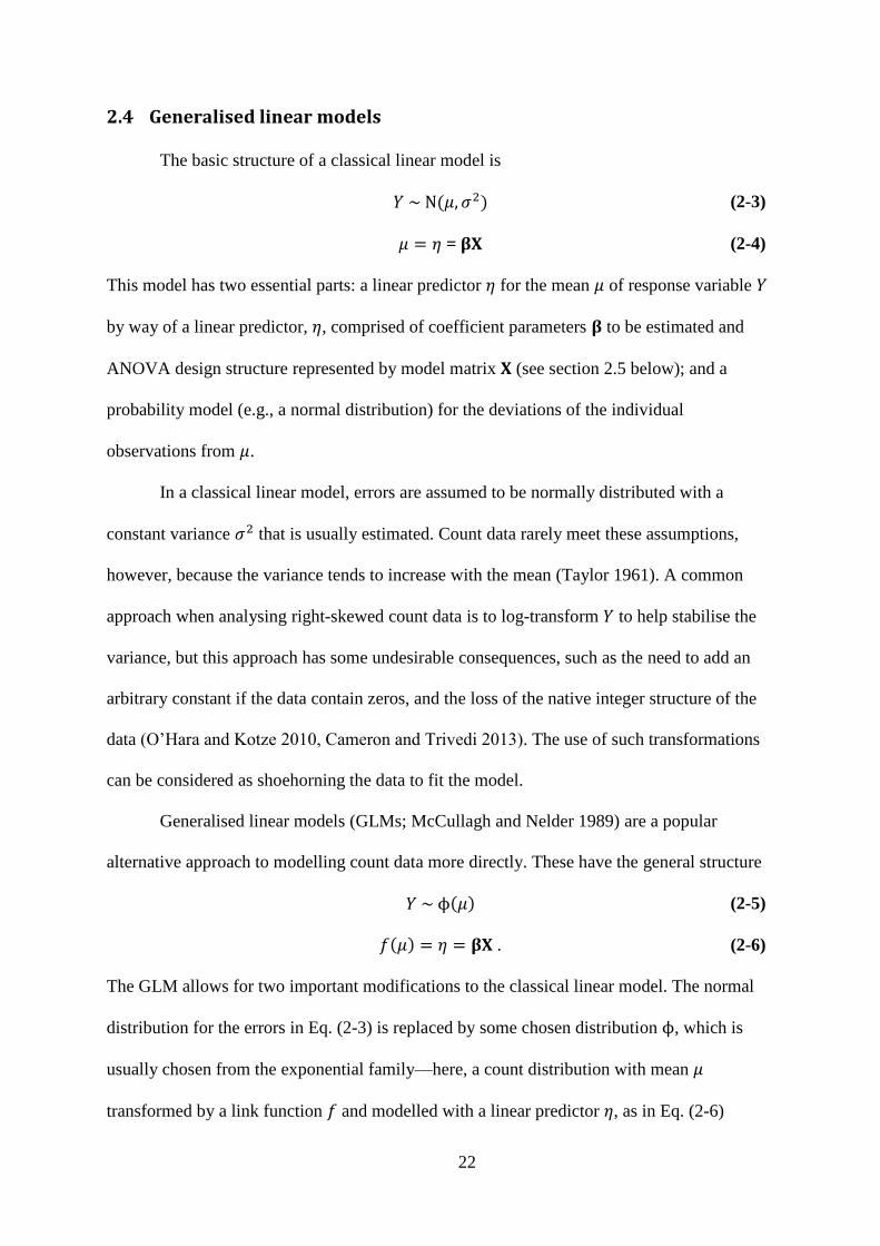
22
2.4 Generalised linear models
The basic structure of a classical linear model is
𝑌 ~ N(𝜇, 𝜎2) (2-3)
𝜇 = 𝜂 = 𝛃𝐗 (2-4)
This model has two essential parts: a linear predictor 𝜂 for the mean 𝜇 of response variable 𝑌
by way of a linear predictor, 𝜂, comprised of coefficient parameters 𝛃 to be estimated and
ANOVA design structure represented by model matrix 𝐗 (see section 2.5 below); and a
probability model (e.g., a normal distribution) for the deviations of the individual
observations from 𝜇.
In a classical linear model, errors are assumed to be normally distributed with a
constant variance 𝜎2 that is usually estimated. Count data rarely meet these assumptions,
however, because the variance tends to increase with the mean (Taylor 1961). A common
approach when analysing right-skewed count data is to log-transform 𝑌 to help stabilise the
variance, but this approach has some undesirable consequences, such as the need to add an
arbitrary constant if the data contain zeros, and the loss of the native integer structure of the
data (O’Hara and Kotze 2010, Cameron and Trivedi 2013). The use of such transformations
can be considered as shoehorning the data to fit the model.
Generalised linear models (GLMs; McCullagh and Nelder 1989) are a popular
alternative approach to modelling count data more directly. These have the general structure
𝑌 ~ ϕ(𝜇) (2-5)
𝑓(𝜇) = 𝜂 = 𝛃𝐗 . (2-6)
The GLM allows for two important modifications to the classical linear model. The normal
distribution for the errors in Eq. (2-3) is replaced by some chosen distribution ϕ, which is
usually chosen from the exponential family—here, a count distribution with mean 𝜇
transformed by a link function 𝑓 and modelled with a linear predictor 𝜂, as in Eq. (2-6)

23
above. This method provides a flexible framework for modelling count data, where
distributions appropriate for integer counts, such as the Poisson, can be used for ϕ. For count
distributions, the mean 𝜇 is usually denoted by 𝜆 and modelled via a log-link function, i.e.,
𝑓(𝜇) = log(𝜆) = 𝜂.
The Poisson distribution
A standard model for count data has the errors following a Poisson distribution,
conditional on a fitted mean. The Poisson distribution is charmingly simple, with only a
single parameter giving both the mean and the variance; thus, 𝜇 = 𝜆 = 𝜎2. The basic
structure of the model is
𝑌 ~ Poisson(𝜆) (2-7)
log (𝜆) = 𝜂 = 𝛃𝐗 . (2-8)
While this model may be useful in some circumstances, counts of organisms often fail to
conform to a Poisson distribution, so its utility in ecological contexts is limited. For the
Poisson model to provide an adequate fit, individuals must occur independently of one
another, a property which results in the variance being equal to the mean. However, few
organisms have such disregard for one another (Taylor 1961).
Overdispersion
Two common properties of counts of organisms cause the variance to be greater than
the mean, a condition known as ‘overdispersion’ (Figure 2-2). The first is broadly termed
‘contagion’ (Neyman 1939, Cole 1946). Individuals of many species occur in groups, due to
social behaviour or aggregation within preferred habitat, for example. The result is that,
where you see one individual of a given species, you are highly likely to see more. Counts of
organisms can also be underdispersed, such that the variance is less than the mean, as in cases

24
where individuals avoid each other or maintain mutually exclusive territories of a similar
size. However, underdispersed data are far less common so will not be considered further
here.
Another common source of overdispersion in counts of organisms is due to there
being a greater number of zeros than would be expected from a Poisson distribution (Welsh
et al. 1996, Cunningham and Lindenmayer 2005). Excess zeros may be caused by a variety of
processes, including social behaviour, imperfect detection, or undesirable habitat (see
Chapter 3 for further discussion). Contagion and excess zeros can exist either together or
separately in a dataset of counts (Figure 2-2). It is increasingly acknowledged that using a
Poisson model for overdispersed data yields incorrect estimates of cell means and uncertainty
in parameters, potentially leading to false conclusions and inappropriate management
decisions (Potts and Elith 2006).
Patterns in the occurrence of individuals in time and space are governed by ecological
processes, and ecological data are a product of a sampling and observational processes
superimposed on the resulting patterns (see Chapter 3). The sampling design thus plays an
important role in determining the way counts can be modelled. Many complicating issues,
such as overdispersion and zero inflation, might be avoided if sampling units are sufficiently
large (e.g. by using a unit of 5-by-5 squares to sample from Figure 2-2D). Indeed, if the
sampling unit (and thus the mean count) is sufficiently large, the data might be adequately
modelled with a normal distribution, yielding much simpler analyses. Smaller sampling units
might be necessary for practical reasons, however, or because of the spatial scale of the
ecological processes that are of interest. Similarly, overdispersion also depends on the model
specification. It is a property of data by reference to a fitted model; the variance of the data
exceeds that which is expected given the model. Much of the extra variation might actually
be driven by some predictable process, in which case it could be accounted for if the right

25
predictor variables were available and included in the model. For example, if the positions of
unsuitable habitat were known, including the suitability of habitat explicitly as a predictor in
the model might remove the need to model excess zeros; they would be accounted for by a
shift in the predicted mean.
Figure 2-2. An illustration of overdispersed counts in a spatial context, by way of contagion
and excess zeros. The points in panel A are randomly distributed without contagion or excess
zeros; thus, counts take from the underlying squares would not be overdispersed (the variance
would equal the mean). Note that panel C contains a greater number of empty cells than panel
A, illustrating that more zeros can arise through contagion alone without any explicit process
that produces excess zeros (Warton 2005).

26
The negative binomial distribution
The negative binomial distribution is a popular alternative to the Poisson for
modelling overdispersed counts (Bliss and Fisher 1953, Taylor et al. 1979, White and
Bennetts 1996). The negative binomial distribution may be parameterised with a mean (𝜇 =
𝜆) and a dispersion parameter (𝜅), as in
𝑌 ~ Negbin(𝜆, 𝜅) (2-9)
log (𝜆) = 𝜂 = 𝛃𝐗 . (2-10)
Like for a Poisson GLM, the log-link function is usually used to model 𝜆 with a linear
predictor, while 𝜅 is usually estimated as a constant (but see Jørgensen 1997). The variance
of a negative binomial distribution is given by 𝜎2 = 𝜆 + 𝜆2/𝜅, a function of both 𝜆 and 𝜅.
The negative binomial results from a mixture distribution: specifically, the mean parameter of
a Poisson is itself a random variable drawn from a gamma distribution. Low values of 𝜅 are
associated with higher levels of overdispersion and, as 𝜅 becomes large, the negative
binomial converges to a Poisson distribution.
The Poisson lognormal
Another approach that allows for overdispersion in counts is the Poisson lognormal
mixture distribution, where the mean of a Poisson distribution is drawn from a log-normal
distribution. In a generalised linear mixed model (GLMM), this can be achieved by adding an
observation-level random effect to the linear predictor on the log-transformed scale (Elston et
al. 2001) as follows
𝑌 ~ Poisson(𝜆) (2-11)
log (𝜆) = N(𝜂 = 𝛃𝐗, σε2) (2-12)
where σε2 is the variance of the observation-level random effect. The distribution of 𝜆 is
symmetrical on the log scale, but asymmetrical on the data scale. Thus, a correction is

27
required when calculating mean counts based on 𝜂 or some other function of the fitted
parameters 𝛃; means may be calculated as 𝜇 = 𝑒𝜂+σε2/2. While the negative binomial has
some computational advantages, one major advantage of the Poisson lognormal is that it
extends easily to the multivariate case for simultaneously modelling multiple count response
variables (Aitchison and Ho 1989).
Modelling excess zeros
Allowing for overdispersion by using a negative binomial or Poisson lognormal might
cater sufficiently well to large numbers of zeros without explicitly modelling them in a zero-
inflated model (Warton 2005). However, where excess zeros do need to be modelled
explicitly, the standard approach is to mix a base count distribution with a Bernoulli
distribution (Lambert 1992). Thus, a general zero-inflated random variable for counts may be
defined as
𝑌 ~ {
0 with probability π Ψ(𝜆) with probability 1 − π
(2-13)
where π is the probability of an excess zero and Ψ is the base distribution for the counts,
often a Poisson or negative binomial. Here, the mean of the Poisson or negative binomial, 𝜆,
is not the overall mean but the mean conditional on an excess zero not occurring. In a zero-
inflated model, the overall mean count is a function of both 𝜋 and 𝜆, given by
𝜇 = (1 − 𝜋)𝜆 . (2-14)
A zero-inflated mixture model can be thought of as a two-step process: a Bernoulli
distribution first determines whether an excess zero occurs (with probability π); then, if not,
Ψ is used to generate a count (Ghosh et al. 2006). Under the “mixture” zero-inflated model, a
zero may arise through either the Bernoulli process (as an excess zero), or through the base
distribution Ψ (as a base zero). An alternative approach, called “conditional” zero inflation,
or a “hurdle” model, allows zeros to be generated only through the Bernoulli process by

28
truncating the base distribution to have a minimum value of one. The conditional model has
been advocated in ecology when zeros are thought to arise from only a single source (Martin
et al. 2005), though I consider such detailed knowledge of the causes of zeros to be rare (see
Chapter 3). The conditional model does have advantages, such as orthogonality of the
statistical processes leading to zeros vs non-zero counts, as well as the ability to model fewer-
than-expected zeros. However, the mixture zero-inflated approach has much to recommend
it; in most cases where there are excess zeros, there are multiple (and unknown) sources of
zeros and the mixture model will most likely be able to reflect the range of ecological and
sampling processes giving rise to zeros in the data.
Models for 𝝅, the probability of excess zero
Typically, 𝜆 is modelled as before, using a GLM of predictors and a log link function
𝑓(𝜆) = log(𝜆) = 𝜂 = 𝛃𝐗 (2-15)
Zero inflation can be incorporated into the model in one of several ways. In increasing order
of complexity, the first option is to simply model 𝜋 as a constant
𝜋 = 𝛼 , (2-16)
where 𝛼 is a parameter to be estimated. This method adds only a single parameter to the
model and assumes a constant rate of excess zeros across the whole dataset. Secondly, where
the occurrence of excess zeros is related to 𝜆, the mean of the conditional counts, the “linked”
method introduced in Chapter 4 of this thesis (and in Smith et al. 2012) can provide a
parsimonious alternative. With this approach, zero inflation is linked directly to the
conditional mean by the linear function
𝑔(𝜋) = 𝛾0 + 𝛾1𝑓(𝜆) . (2-17)
This adds only two parameters to the model, namely 𝛾0 and 𝛾1, which determine the shape of
the relationship between 𝜆 and 𝜋, each transformed by their link functions 𝑓(𝜆) and 𝑔(𝜋),

29
usually the log and the logit, respectively. This method allows 𝜋 to take a range of values
while adding only two extra parameters to the model. It assumes that the processes
underlying the excess zeros and, thus, their relationship with the predictor variables, are
similar to those that drive the counts. If this is not the case and greater flexibility is required,
a third option is to use a separate linear function for the excess zeros, as in
𝑔(𝜋) = ζ (2-18)
ζ = 𝛂𝐙 . (2-19)
Here, ζ is a linear predictor distinct from η, comprised of coefficient parameters 𝛂 and
predictor variables 𝐙. The parameters 𝛂 and 𝛃 are different, though 𝐙 may or may not be the
same as 𝐗. As 𝜋 is a binary variable, an appropriate link 𝑔 would be the logit function,
though probit or log link functions might also be used. This method provides the flexibility
for the degree of zero inflation to follow patterns distinct from that of the base counts of
abundances, which might be useful where different mechanisms are involved in driving
excess zeros as opposed to base-count values in the observed data.
2.5 Analysis of variance and mixed-effects models
ANOVA as a linear model
Many ecological studies have a structured hierarchical sampling design that involves
one or more treatments or factors of interest in combination with sampling units measured at
multiple spatial and/or temporal scales. Each level of the hierarchy potentially introduces
variation that can be modelled concurrently alongside treatments or other factors.
A Poisson GLM is usually expressed in terms of the 𝑝 = 1, … , 𝑃 coefficients 𝛃 and
predictor variables 𝐗, using 𝑖 = 1, … , 𝑁 to index individual data points,
𝑌𝑖 ~ Poisson(𝜆𝑖) (2-20)

30
log 𝜆𝑖 = 𝜂𝑖 = β0 + β1𝑋1𝑖 + β2𝑋2𝑖+. . . +β𝑃𝑋𝑃𝑖 (2-21)
This form of the linear model can describe either a regression model or an ANOVA model.
Consider a parameterisation where the coefficients (β𝑝) each represent the effect of a single
level of a factor. The levels are coded as binary “dummy” 𝑋 variables which take the value of
one or zero according to whether the observation does or does not belong to that level,
respectively. Higher-order terms in an ANOVA design (e.g., nested terms in a hierarchy or
interaction terms) can also be defined using appropriate dummy variables and associated
coefficients (e.g., see Appendix C in Legendre and Anderson 1999). When coded in this way,
the coefficients can be grouped into batches according to the term to which they belong
(Gelman 2005).
An ANOVA linear model can be expressed concisely in a form that reflects the batch
structure of the coefficients, where “batches” of effects correspond to particular terms
(sources of variation) in the ANOVA model. For example, a Poisson GLM for the MPA
study design introduced in Section 2.3 may be expressed as
𝑦𝑗𝑘𝑙𝑖 ~ Poisson(𝜆𝑗𝑘𝑙) (2-22)
log 𝜆𝑗𝑘𝑙 = 𝜂𝑗𝑘𝑙 = β0 + 𝑀𝑗 + 𝐿𝑘 + 𝑀𝐿𝑗𝑘 + 𝐴𝑙(𝑗𝑘) (2-23)
Here, the 𝑦𝑗𝑘𝑙𝑖 observations are explicitly associated with a single level for each factor
(𝑀𝑗, 𝐿𝑘, etc.), with the subscript 𝑖 ∈ {1, 2, 3, 4} now indexing replicates within each
combination of levels. The coefficients are grouped into terms, with 𝑀𝑗, 𝐿𝑘, and 𝐴𝑙(𝑗𝑘)
representing the main effects of MPA, Location, and Area, respectively, and 𝑀𝐿𝑗𝑘 denotes
the interaction effects between MPA and Locations (e.g., differences in the MPA effects
among locations or vice versa). The indexing in the term for Areas, 𝐴𝑙(𝑗𝑘), reflects the key
idea that this factor is nested within combinations of levels of 𝑀 and 𝐿. In comparison, the
full, unconstrained model for the MPA design would take many lines to express using the
long format in Eq. (2-21).

31
Fixed vs random effects
In ANOVA models, factors may be treated as fixed or random, and various guidelines
have been put forth for choosing how to treat any given factor (e.g., as reviewed by Gelman
2005). In ecological studies, factors for which the levels represent particular treatments or
effects that of particular interest (such as the MPA factor in our example) are usually treated
as fixed, whereas spatial or temporal replicates (such as the Locations and Areas) are usually
treated as random.
Treating a term as fixed or random affects how it is structured in the model and, in
particular, how the batch of coefficients are collectively constrained. For a fixed term in a
one-way ANOVA, the estimate of the mean for any particular level is simply the mean of
those units belonging to that level. Fitting a parameter for each level (along with an overall
intercept, β0), however, results in overparameterisation—a given term should only have so
many stochastic parameters as it has degrees of freedom—so some constraint is required.
When fitting models using an R package such as lme4 and MCMCglmm, these constraints are
coded implicitly for each factor as a matrix of contrasts. When using BUGS, the constraint is
usually coded explicitly, typically by one of the following two methods (Ntzoufras 2011). Let
factor F be a fixed factor with coefficients β𝑐(𝐹)
where 𝑐 = {1, … , 𝐶} represents the levels of
F. If a “corner constrait” is used, one coefficient is set to zero and the remaining 𝐶 − 1
coefficients are stochastic and assigned a noninformative prior distribution, e.g.,
β𝑐
(𝐹){
= 0 𝑐 = 1 ~𝑁(0,100) 𝑐 = {2, 3, … 𝐶}
(2-24)
This has the effect of treating level one as the base, with the other β(𝐹) coefficients
representing the difference from that base. This approach can be useful where, e.g., there are

32
multiple treatments to compare vs a single control. Alternatively, a “sum-to-zero” constraint
may be used, where one level is set to the negative sum of the others, as in
β𝑐(𝐹)
{= − ∑ β𝑐
(𝐹)
𝐶
𝑐=2
𝑐 = 1
~ 𝑁(0,100) 𝑐 = {2, 3, … 𝐶}
(2-25)
For a two-level factor, such as the factor 𝑀 in our MPA example, a single β(𝑀) is estimated.
The effect of one level is represented by β(𝑀) (the effect of being inside the MPA) and the
other by –β(𝑀) (the effect of being outside the MPA), with β0 representing the overall mean
across all of the data. The sum-to-zero approach is convenient because it can allow for more
straightforward calculations of certain quantities of interest. For example, one could estimate
the overall median of counts inside the MPA example, ignoring all other factors in the model,
as
λ∙1∙ = 𝑒β0+𝑀1 = 𝑒β0+β(𝑀) . (2-26)
For interactions among fixed terms, constraints may be applied for a fixed factor within each
level of the other factor (or combination of factors).
For a random factor 𝑅, on the other hand, the levels and their associated parameters
are assumed to be a random sample drawn from a population of potential levels (e.g., such as
a normal distribution), i.e.,
β𝑐(𝑅)
~ 𝑁(0, 𝜎𝑅2) ∀ 𝑐 (2-27)
𝜎𝑅2 ~ 𝜔(. ) (2-28)
where 𝜎𝑅2 is a parameter representing the variance component for factor 𝑅, which is assigned
some prior distribution 𝜔 and estimated (Gelman 2005, McCulloch et al. 2008). Estimating a
variance component on top of the error variance introduces a hierarchical structure to the
parameters. Information about the distribution of the batch parameters is shared amongst the
levels, often referred to as “borrowing strength” across the groups. An important consequence

33
of this is that the estimates of the β coefficients are “shrunk” toward zero. The constraints
commonly applied to fixed effects are not required for random effects; while the population
mean is assumed to be zero, there is no guarantee that the particular sample of levels obtained
will have a mean of exactly zero. For fixed factors, the super-population variance is
effectively set to ∞, and no shrinkage occurs (Gelman 2005). Thus, treating an effect as
random, rather than fixed, results in more conservative estimates of the effects of being in a
particular level (Figure 2-3).
The degree of shrinkage is generally greater when the data contain more information
about the distribution of levels than about the effects of the individual levels. This can occur
when there are few replicates within each level but a large number of levels, and when the
among-level variance is small relative to the within-level variance (Gelman and Hill 2007).
The degree of shrinkage is also influenced by the prior distribution placed on 𝜎𝑅2 (or, more
commonly, on 𝜎𝑅) for the random effect, though this influence will generally be negligible
for data-rich models. The use of a non-negative distribution precludes negative estimates of
variance components. A range of distributions have been suggested for this prior. In cases
where the number of levels is large, Gelman (2006) and Gelman & Hill (2007) suggest an
uninformative uniform prior distribution between zero and a sufficiently large upper limit for
𝜎𝑅. In this case, the prior distribution is less important because the posterior distribution, and
the degree of shrinkage, will largely be driven by the data via the likelihood.
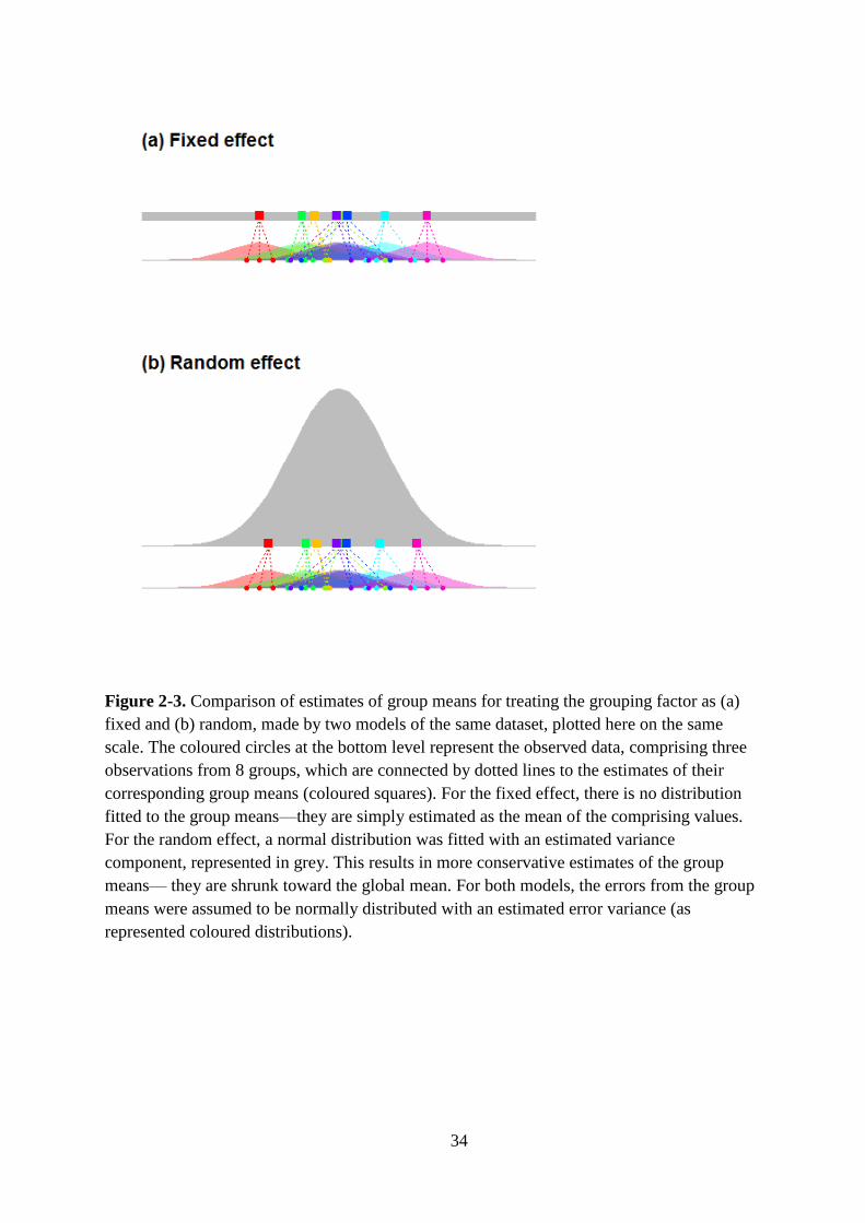
34
Figure 2-3. Comparison of estimates of group means for treating the grouping factor as (a)
fixed and (b) random, made by two models of the same dataset, plotted here on the same
scale. The coloured circles at the bottom level represent the observed data, comprising three
observations from 8 groups, which are connected by dotted lines to the estimates of their
corresponding group means (coloured squares). For the fixed effect, there is no distribution
fitted to the group means—they are simply estimated as the mean of the comprising values.
For the random effect, a normal distribution was fitted with an estimated variance
component, represented in grey. This results in more conservative estimates of the group
means— they are shrunk toward the global mean. For both models, the errors from the group
means were assumed to be normally distributed with an estimated error variance (as
represented coloured distributions).

35
However, if there are only a few levels (fewer than 5), the uniform prior tends to lead to high
estimates of 𝜎𝑅, with the posterior distribution having an excessively large tail. In this case, a
weakly informative prior distribution for 𝜎𝑅 is recommended, such as the half-Cauchy, which
provides an appropriate balance between discouraging large values and behaving well near
zero (Gelman 2006). An appropriate value of the scale parameter must be chosen for the half-
Cauchy to reflect plausible values of 𝜎𝑅 (Figure 2-4). The For models of count data in which
means are modelled on the log scale and thus the standard deviation of the effects will be
relatively small, the standard half-Cauchy (i.e., with a scale parameter of one, equivalent to a
half-Student’s t distribution with one degree of freedom) might be reasonable. However,
larger values of the scale parameter might be appropriate for identity-link models, where
effect sizes might be larger (Gelman 2006).
Figure 2-4. Density of the Cauchy distribution with scale-parameter values of 1–3 (x-axis
truncated at 8).

36
Presenting variance components
The results of classical ANOVA models have historically been presented as a table of
coefficients (presenting, for each coefficient, a point estimate with standard errors and a p-
value for the null hypothesis of the true value of the coefficient being zero), or an ANOVA
table (presenting, for each term, the mean square, F-ratio of observed to expected mean
squares, and the corresponding p-value testing the frequentist null hypothesis of all the
coefficients associated with a given term being exactly equal to zero). For large models, a
table of coefficients is cumbersome due to the sheer number of individual parameters and,
besides, interest often lies primarily at the level of whole terms—i.e., in the batches of
coefficients rather than in individual coefficients. Classical ANOVA summaries require the
specification of correct expected mean squares for each term, which are non-trivial to derive
for complex mixed models, particularly for unbalanced designs (Graham and Edwards 2001,
Searle et al. 2009). Moreover, many authors in ecology, including non-Bayesians, have
criticised the hypothesis-testing approach (Reckhow 1990, Johnson 1999, Anderson et al.
2000). Tests of hypotheses are dependent on both the magnitude of the effect and the amount
of data informing it, and while p-values may indicate the weight of evidence against a null
hypothesis, they do not directly inform us about the magnitude of effects, nor do they provide
a basis for comparing the relative sizes of the different component sources of variation
(terms) in the model.
Many have argued that variance components provide a more useful summary of an
ANOVA model when the primary goal is to quantify and compare the magnitude of effects
for each term (Graham and Edwards 2001, Gelman 2005, Qian and Shen 2007, Qian et al.
2009, 2010, Hector et al. 2011). In a Bayesian model, it is straightforward to estimate
multiple variance components in complex multi-factor models, even for unbalanced designs,

37
and to summarise relative sizes of variance components with point estimates and uncertainty
intervals. When Gelman (2005) championed this approach, he distinguished two types of
variance component: the finite-population variance (𝑠2), which is estimated directly from the
levels represented in the dataset, and the super-population variance (𝜎2) of all levels, which
includes the notion of uncertainty associated with predicting the coefficients for unobserved
levels, as appropriate for random effects. Gelman (2005) recommended comparing the
magnitude of effects in a model using the finite-population standard deviations (𝑠 = √𝑠2).
Finite-population standard deviations have the advantage that they may be estimated for both
fixed and random effects. This quantity can be calculated directly from the estimated
coefficients for the levels,
𝑠 = √∑ (β𝑐−β)2𝐶
𝑐=1
𝐶−1 ,
(2-29)
which reduces to
𝑠 = √∑ β𝑐
2𝐶𝑐=1
𝐶−1
(2-30)
under the sum-to-zero constraint for fixed effects. In a Bayesian analysis, 𝑠 may be calculated
at each iteration of the MCMC and summarised and compared with point and interval
estimates, usually the median and 0.025th and 0.975th quantiles. Gelman (2005) introduced a
graphical method of displaying these summary statistics, which has been employed in the
ecological literature (e.g. Qian and Shen 2007, Hector et al. 2011, Irwin et al. 2013, Smith et
al. 2014).
While the finite-population standard deviations provide useful quantities for
comparing the magnitude of effects across the terms in the model, it is important to realise
that the decision of which factors are treated as fixed vs random will influence this quantity.
Random effects will be shrunk toward zero in accordance with the estimated super-
population variance component 𝜎𝑅2, with the degree of shrinkage being more extreme for

38
smaller estimates of 𝜎𝑅2. In contrast, fixed effects are estimated with no shrinkage, essentially
fixing 𝜎2 at infinity (see Gelman 2005). In some sense then, fixed and random factors are
compared on an unequal footing. This might be considered reasonable under the assumption
that random effects are drawn from a population in which some (most) levels remain
unobserved, whereas all levels of interest for a fixed effect are included in the model.
The use of a link function, such as the usual log link for count data, for mapping the
mean to the linear predictor complicates interpretation of the model parameters. In a classical
linear model, the model parameters reflect the original measurement scale of the data.
However, where a link function is used, parameters are estimated on a transformed scale; for
count data, this is usually the log scale. Additive terms in a model fit on the log scale are
multiplicative on the scale of the original data, and thus the interpretation of any particular
effect requires some care. Normally distributed random effects fit on the log scale are log-
normally distributed on the data scale, and the degree of variance among levels therefore
depends on the fitted mean. For example, in the MPA scenario, the random term Area is
nested within MPA status-by-Location. The fitted mean count might be much larger inside vs
outside MPAs, so fitting a common variance for Area would assume that there is greater
variation among areas inside vs outside MPAs. Likewise, for logistic regression models (such
as those predicting excess zeros in a zero-inflated model), variance components estimated on
the logit scale correspond to different variances on the scale of the data according to the fitted
probability (𝜋); for a given logit-scale variance, the data-scale variance is greatest near 𝜋 =
0.5 and decreases as 𝜋 approaches either 0 or 1. Comparisons of estimated variance
parameters, such as finite-population standard deviations, among terms in a model is,
however, valid in a relative sense, with the assumption that effects are indeed additive and
comparable within the link-transformed scale. Meaningful interpretation of the estimated

39
values of variances in the context of generalised linear mixed models does require careful
consideration; see Nakagawa & Schielzeth (2010, 2013) for some options.
2.6 Model fitting
It is straightforward to fit a traditional ANOVA model to a balanced dataset with
normally-distributed errors. Estimating the parameters, including variance components, can
be done arithmetically using sums of squares, though methods based on maximum likelihood
(ML), restricted maximum likelihood (REML), and their approximations, may also be used
for mixed-effects models with normal error structures (Searle 1995). For more complicated
models, such as those incorporating non-standard error distributions (to account for
overdispersion and/or excess zeros), unbalanced designs, and multiple crossed or nested
random effects, fitting via likelihood-based approaches can be difficult or even intractable
(McCulloch et al. 2008, Bolker et al. 2009).
Modellers in ecology and other sciences are increasingly turning to Bayesian MCMC
methods and model-scripting languages, such as BUGS (Lunn et al. 2000, 2013) and Stan
(Stan Development Team 2014), because they provide researchers with increasing flexibility
to fit complex models. A sample of posterior parameter values, as provided by MCMC, is a
convenient and flexible basis for statistical inference. When fitting a model via MCMC, there
is a number of steps that must be taken in order to ensure that the sample adequately
represents the true posterior distribution and can thus be used as a basis for inference. Some
brief guidelines are provided in the sections below (see texts by, e.g., Lunn et al. 2013,
Gelman et al. 2014a, for more thorough treatments).
Initial values, convergence, and burn-in

40
Three or more implementations of the MCMC algorithm (i.e., multiple “chains”) are
often run simultaneously to aid with diagnosing the validity of the posterior sample, after
which they may be pooled for inference. MCMC is iterative and requires initial values for the
full set of stochastic parameters. Many computer programs can provide sensible initial values
for relatively simple models. For more complex models, it is generally advised that initial
values should be specified manually to ensure, firstly, that they are on an appropriate scale
and, secondly, that they are disparate among the chains. Doing so will minimise the risk that
the algorithm becomes stuck in a particular part of the parameter space and fails to lead to
sensible combinations of values under the true posterior distribution.
All going well, after some number of iterations, the chains will converge upon the
posterior distribution, allowing subsequent values to be used for inference. The parameter
values prior to convergence—the “burn-in”—must be discarded. More complex models
generally require longer burn-in periods. Where computational time is not a major issue, the
burn-in number may be set arbitrarily high (some thousands, tens of thousands, or more);
nonetheless, checking for convergence is critical. Convergence can be checked informally by
examining the “trace” plot—a plot of the ordered parameter values along each chain. The
burn-in period is usually clearly visible as the traces track from their initial values toward a
particular range, within which they subsequently remain. When multiple chains are used,
their behaviour should be indistinguishable. Convergence can be quantified more formally
using statistics that are trivial to calculate, the most common being the Brooks-Gelman-Rubin
��-statistic (Gelman and Rubin 1992, Brooks and Gelman 1998), which compares the within-
and among-chain variability for a parameter. Values of �� around 1 suggest convergence, and
a common rule of thumb decrees that �� < 1.05 is satisfactory, though neither this nor any
other method can totally guarantee convergence.

41
MCMC efficiency
The accuracy of an MCMC approximation of the posterior distribution of parameters
relies on obtaining a large sample of independent values. Autocorrelation among consecutive
values in the chain is always present to some degree, and is generally important in all but the
most simple and balanced models (Lunn et al. 2013). At best, it is negligible, and trace plots
of the parameter values (after discarding the burn-in) show no apparent serial correlation, i.e.,
they are “well mixed”. At worst, the trace takes a “snake-like” appearance, indicating that
mixing is poor. The way in which a model is parameterised can affect how well it mixes. In
particular, mixing can be improved for hierarchical models by way of “hierarchical centring”
(Gelfand et al. 1995), such that, for example, the model
𝑦𝑖𝑗~𝑁(𝜇0 + 𝛼𝑖, 𝜎𝜖2) 𝛼𝑖~𝑁(0, 𝜎𝛼
2) (2-31)
may mix better when specified (equivalently) as
𝑦𝑖𝑗~𝑁(𝜇𝑖, 𝜎𝜖2) 𝜇𝑖~𝑁(𝜇0, 𝜎𝛼
2) . (2-32)
Where it is important, autocorrelation reduces the “efficiency” of the MCMC sample.
An inefficient MCMC sample contains less information about the posterior distribution than
would be indicated by the ostensive size of the MCMC sample. In this case, to obtain an
adequate posterior approximation, the MCMC should be run for longer. It is common
practice to “thin” the chain—keeping only one value out of, say, 10, 100, or 1000 or more
iterations—to decrease the degree of autocorrelation and increase the efficiency of the
retained sample. A useful statistic for quantifying the amount of information in an MCMC
sample is the “effective sample size”, which estimates the amount of independent information
contained in the sample values. This value is routinely reported by BUGS and many similar
programs. As a general guide, an MCMC sample of around 4,000 independent values is
required to reliably estimate a 95% credible interval for a parameter with a well-behaved
posterior distribution (Lunn et al. 2013).

42
The “zeros-trick”
BUGS has a wide range of built-in probability distributions that can be used to specify
the errors from fitted models and assign prior distributions to stochastic parameters. Yet, a
modeller may wish to specify a probability distribution that is not offered in BUGS. In this
case, one can explicitly specify a likelihood function and use the so-called “zeros trick”,
effectively allowing any distribution to be used.
Let ℒ𝑖 = 𝑓(𝑦𝑖|𝜃) be the desired likelihood for data 𝑦𝑖 given parameters 𝜃. To use the
zeros trick, one specifies a set of dummy data observations with length 𝑛, each with a value
of zero, i.e.,
𝑧𝑖 = 0 ∀ 𝑖 = 1, … , 𝑛 (2-33)
The 𝑧𝑖 dummy observations are then modelled using a Poisson distribution with mean
parameter 𝜈𝑖.
𝑧𝑖 ~ Poisson(𝜈𝑖) (2-34)
Thus, the likelihood contribution for 𝑧𝑖 is
𝑃(𝑧𝑖 = 0) = 𝑒−𝜈𝑖 (2-35)
If one assigns 𝜈𝑖 to be the negative log of the desired likelihood ℒ𝑖 (plus an arbitrarily large
constant, 𝑐, to ensure 𝜈𝑖 remains positive)
𝜈𝑖 = − log ℒ𝑖 + 𝑐 (2-36)
𝑐 = 10,000 (2-37)
then ℒ𝑖(𝑦𝑖|𝜃𝑖) may be specified explicitly using any function of the data 𝑓 and parameters.
Thus, the correct likelihood for the data is obtained (p. 204, Lunn et al. 2013) as
𝑃(𝑌𝑖 = 𝑦𝑖) = ℒ𝑖 = 𝑒−𝜈𝑖+𝑐
= 𝑃(𝑧𝑖 = 0) + 𝑒𝑐
∝ 𝑃(𝑧𝑖 = 0)
(2-38)

43
For example, the built-in implementation of the negative binomial distribution in
BUGS is formulated via an alternative parameterisation, using probability parameter 𝑝 =𝜅
𝜅+𝜆
instead of the mean 𝜆, and allowing only (positive) integer values for the dispersion
parameter 𝜅, which is not appropriate for modelling most count data. Instead, one could
specify ℒ𝑖 to be the negative binomial likelihood
ℒ𝑖 =Γ(𝑦𝑖+𝜅)
Γ(𝜅)𝑦𝑖!(
𝜆𝑖
𝜆+𝜅)
𝑦𝑖
(1 +𝜆𝑖
𝜅)
−𝜅
(2-39)
A model can then be articulated for 𝜆𝑖 as a function of predictor variables 𝑥𝑖 and model
parameters 𝜃, and with prior distributions assigned to 𝜃. An appropriate non-negative, non-
integer prior distribution may be assigned to the dispersion parameter (e.g.,
𝜅 ~ Gamma(10−4, 10−4), 𝜅 ϵ (0, ∞)), thereby avoiding the problem of BUGS’ inbuilt
function allowing only integer values. The zeros trick can also be used to avoid problems
with inbuilt model selection tools when using mixture distributions, such as zero-inflated
count distributions, as described in the next section.
2.7 Model evaluation and selection
To make accurate inferences, a statistical model should reflect the system that
produced the data. Ideally, the predictor should articulate an appropriate relationship between
the data and all potentially important sources of variation (or, at least, those that are known
and measurable), the error structure should adequately account for the deviations from the
predictor, and prior distributions should include the plausible ranges of values for the model
parameters before the data were observed. For most data analyses, it is rare that the structure
of the true model that generated the data is known, so several different models are fit.
Evaluating and comparing the plausibility of the set of fitted models is an essential part of the
modelling process. Indeed, inference based on a model that does not adequately fit the data

44
will be inaccurate. This section reviews some methods for assessing and selecting models that
are common in Bayesian MCMC analysis.
Assessing model fit
Posterior Predictive Checking (PPC; see Gelman et al. 2014a) has become standard
methodology for assessing the plausibility of a model (given the data at hand) in a Bayesian
analysis. The rationale for PPC is that, if the model fits well, the observed data should be
consistent with data simulated from the model. This comparison is enabled by simulating a
set of replicate datasets using the posterior distribution of the model parameters, termed 𝑦𝑟𝑒𝑝:
𝑝(𝑦𝑟𝑒𝑝|𝑦) = ∫ 𝑝(𝑦𝑟𝑒𝑝|𝜃) 𝑝(𝜃|𝑦) 𝑑𝜃
(2-40)
If the observed data are substantively different from those generated by the model, it can be
argued that the model is unlikely to have produced the observed data.
Comparison is usually done by calculating a summary statistic 𝑇 for both the
observed dataset (𝑇(𝑦)) and for each of the replicated datasets 𝑇(𝑦𝑟𝑒𝑝). Concern is raised
regarding the fit of the model if there is a discrepancy between 𝑇(𝑦) and the distribution of
𝑇(𝑦𝑟𝑒𝑝), such that 𝑇(𝑦) is located outside the normal range of the 𝑇(𝑦𝑟𝑒𝑝) values. The
discrepancy can be summarised using a posterior predictive p-value, which is the probability
that the replicated data are more extreme than the observed data; it is calculated as the
proportion of 𝑇(𝑦𝑟𝑒𝑝) values that are more extreme than the observed 𝑇(𝑦):
𝑝 = 𝑃(𝑇(𝑦𝑟𝑒𝑝, 𝜃) ≥ 𝑇(𝑦, 𝜃)|𝑦) (2-41)
In practice, we are used to seeing low p-values so one might consider the minimum of 𝑝 and
1 − 𝑝; very low values of either is cause to doubt the fit of the model. A range of discrepancy
measures should be chosen to reflect various aspects of the model, and particularly those that
are relevant to the scientific objective of the study. Measures might include the overall mean,

45
variance, minimum or maximum of the data or, if the data are counts, the total count or the
number of zeros.
PPC is a useful method for ruling out models that do not adequately fit the data.
Crucially, if no model in the candidate set appears consistent with the data, then none should
be relied upon for inference. In this case, the structure and assumptions of the models fit thus
far should be re-examined, and a broader range of alternative models should be assessed.
Although PPC can be used to discard unsupported models and corroborate more formal
model selection processes, it does not provide a clear basis for model selection as clearly
more than one model might be capable of producing plausible replicate datasets that are
consistent with the observed dataset.
Model selection
A decision might be required as to which models of a set of candidates should be
presented as “best”. Methodology for selecting models remains an important and challenging
area of research. Recent decades have seen a rise in the development and use of information
criteria. Conveniently, information criteria provide a single number for each model that can
be directly compared, generally with smaller values indicating greater support for a given
model. They are also generally trivial to calculate, combining some measure of model fit,
often the deviance, with a penalty for model complexity based on the number of fitted
parameters in the model.
The deviance is a measure of the unexplained variation in a dataset given a model
(McCullagh and Nelder 1989). The deviance is used in the context of GLMs, providing a
generalisation of the normal-theory sum of squared errors for non-normal distributions. For
any likelihood function ℒ = 𝑓(𝑌|𝜃), one can calculate the deviance
𝐷(𝜃) = −2 log ℒ (2-42)

46
The deviance of a model is usually calculated by reference to the fitted values of the
parameters, 𝐷(𝜃).
The deviance measures the inaccuracy of a model’s fit to the observed data (also
called “within-sample data); a larger deviance indicates a poorer fit. The deviance does not in
itself provide a measure of a model’s predictive inaccuracy for unobserved (out-of-sample)
data, i.e., data that might arise from the same system that were not used to fit the model. In
general, a more complex model (one with more parameters) will always provide a better fit to
the observed data (and, thus, have lower deviance), but not necessarily to unobserved data. A
better estimate of a models general predictive performance can be obtained through cross
validation, where a proportion of the data is withheld and used as an independent test set
(Geisser and Eddy 1979). In k-fold cross validation, the data are divided into k groups, and
each is withheld in turn and used to calculate the deviance from model predictions. If k is set
to 1, every single observation is withheld in turn; this method is known as leave-one-out
cross-validation (LOO-CV). Calculating the deviance using withheld data provides a more
rigorous basis for model comparison; however, this general method is computationally
expensive, and it can be difficult to implement when few data are available.
Information criteria provide some useful and (usually) computationally less-expensive
alternatives to cross validation. Perhaps the most well-known is Akaike’s Information
Criterion (AIC; Akaike 1973), which has been used extensively in ecology since it was
popularised by Burnham and Anderson (2002). AIC may be calculated as
AIC = 𝐷(𝜃) + 2𝑝 (2-43)
where 𝑝 is the number of parameters in the model and 𝐷(𝜃) is the within-sample deviance
obtained using the estimated values of the parameters (e.g., as estimated using maximum
likelihood). It can be seen as a deviance with a penalty to account for the fact that it is
calculated from within-sample data, rather than independent data. In the limit (i.e., at very

47
large sample sizes), the model with the lowest AIC score is expected to have the lowest
predictive inaccuracy for out-of-sample data (Shibata 1976, Stone 1977, Gelman et al.
2014b). There are two problems with using AIC in the context of Bayesian hierarchical
modelling: Bayesian model parameters 𝜃 have a posterior distribution which is ignored by
simply using only the fitted values (𝜃), and the simple insertion of the nominal number of
model parameters is inappropriate for anything more complex than linear models with flat
prior distributions (Gelman et al. 2014b).
Thus, in contrast, the Deviance Information Criterion (DIC; Spiegelhalter et al. 2002)
has become widely used in Bayesian modelling. It is trivial to calculate from MCMC
samples, and is defined as
DIC = 𝐷(𝜃) + 𝑝𝐷 (2-44)
Here, 𝐷(𝜃) , known as “D bar”, is the mean of the posterior distribution of the deviance. It is
calculated for each MCMC sample drawn, and therefore includes the uncertainty in the model
parameters. The penalty term, 𝑝𝐷, is an estimate of the “effective” number of parameters in
the model. This distinguishes the DIC from alternative criteria, such as the Akaike
Information Criterion (AIC), in that it estimates the dimensionality of the parameter space
using the posterior distribution, rather than using a simple count of the (nominal) number of
parameters, 𝑝. This is important for hierarchical models, in which the parameters are not
independent of one another and, thus, 𝑝 will generally overestimate the true dimensionality of
the parameter space.
There are various proposed methods for calculating the effective number of
parameters in the model, the most common being
𝑝𝐷 = 𝐷(𝜃) − 𝐷(𝜃) (2-45)
Some potential problems exist for 𝑝𝐷: it, like the AIC, relies on point estimates of the
parameters, 𝜃; it can be negative when the posterior distribution of 𝜃 is non-symmetrical;

48
different values of 𝑝𝐷 can be obtained by reparameterising the model; and 𝑝𝐷 cannot be
calculated when 𝜃 includes a categorical parameter (Lunn et al. 2013). A proposed alternative
estimate of the effective number of parameters is
𝑝𝑉 = Var(𝐷(𝜃))/2 (2-46)
i.e., half of the variance of the posterior distribution of the deviance (Gelman et al. 2014a).
Though 𝑝𝐷 is more numerically stable in some cases, 𝑝𝑉 has the advantages of being easier to
calculate, always positive, avoids point estimates of parameters, and is more robust to
reparameterisations (see comparison on p. 165, Lunn et al. 2013).
More recently, there is growing support for the so-called Widely Applicable (or
Watanabe-Akaike) Information Criterion (WAIC; Watanabe 2010, Vehtari et al. 2015),
which proposes yet more alternative methods for estimating the effective number of
parameters. The method recommended by Gelman et al. (2014a, 2014b), is related to 𝑝𝑉 but,
instead of basing the estimate on the variance of the total deviance, as in Eq. (2-38), it uses
the sum of the variances of the fit to each data point
𝑝WAIC = ∑ Var(log 𝑝(𝑦𝑖|𝜃))
𝑛
𝑖=1
(2-47)
As with 𝑝𝑉, 𝑝WAIC avoids point estimates of the parameters (𝜃). Further, it is argued that the
WAIC is more stable than its alternatives, works well for mixture models, is invariant to
reparameterisations, and is asymptotically equivalent to LOO-CV (Gelman et al. 2014a). The
WAIC does involve additional computations that are not already required for the DIC
(Vehtari et al. 2015; but see Vehtari and Gelman 2014 for implementation in Stan), and while
the WAIC may prove to be as “widely applicable” as the name suggests, further study is
required.
Most MCMC software packages automatically provide “plug-in” values for the
deviance, 𝑝𝐷 or 𝑝𝑉, and the DIC, but these should be used with caution. There are several

49
formulations of the DIC in addition to those given here, and none has been shown to perform
consistently across a broad range of scenarios (Celeux et al. 2006). In the context of
hierarchical datasets and models, it may not be appropriate to calculate the deviance based on
the level of the individual data points 𝑦, as is done by the plug-in deviance and DIC
(Spiegelhalter et al. 2002, Lunn et al. 2013). The priority may instead be to choose a model
that most accurately predicts at a higher level of the hierarchy, such as the site means. In this
case, a site-marginalised version of the DIC may be calculated (Millar 2009).
Care must also be taken when using the DIC for models with a mixture distribution
for the errors. This is often the case when fitting a zero-inflated count distribution, such as the
ZIP. This distribution may be parameterised using a latent Bernoulli parameter, as in 𝑏 in the
following (subscript 𝑖 is suppressed for brevity):
𝑦~Poisson(𝜙)
𝜙 = (1 − 𝑏) ∗ 𝜆
𝑏~Bernoulli(𝜋) .
(2-48)
Here, the occurrence of an excess zero is given by the latent parameter 𝑏, which is modelled
as a Bernoulli distribution, taking the value 𝑏 = 0 with probability 𝜋 and 𝑏 = 1 with
probability 1 − 𝜋, respectively. Where 𝑏 = 0, an excess zero has not occurred and 𝑦 is then
Poisson-distributed with mean 𝜆. The problem with this parameterisation is that the latent
variable 𝑏 is treated as data by the plug-in DIC; the fit of 𝑏 to the Bernoulli distribution will
contribute to the estimated deviance. This problem may be avoided by specifying the
likelihood using the zeros trick as follows (Millar 2009):
𝑧 = 0
𝑧 ~ Poisson(𝜙)
𝜙 = − log ℒ
(2-49)

50
ℒ = {
𝜋 + (1 − 𝜋)𝑒−𝜆 𝑦 = 0
(1 − 𝜋)𝑒−𝜆𝜆𝑦
𝑦! 𝑦 > 0
Models fit using the zeros trick in this way avoids the use of a latent parameter 𝑏. However,
the plug-in DIC scores of models fit using the zeros trick cannot be compared with those fit
using built-in distributions. In this case, one can either use the zeros trick for all models, or
correct the DIC score for models that use the zeros trick (see, e.g., p. 284 of Lunn et al.
2013).
The DIC is a convenient tool for comparing Bayesian models but it clearly has pitfalls
and limitations and it, solely, should not be relied upon for model selection. It can be
informative to examine separately the two components of the DIC—the mean deviance as a
measure of within-sample fit and the effective number of parameters as a measure of
complexity. More complex models should generally have smaller deviance, and 𝑝𝐷 and 𝑝𝑉
should both be less than the nominal number of parameters, 𝑝, for hierarchical models. Model
selection can be informed by these and other approaches, such as PPC. Let common sense
prevail. If a particular model achieves a lower deviance with fewer parameters and appears to
provide better fit to the observed data, it is likely a wise choice.
There are plenty of alternative tools and approaches for model selection (see extensive
review by Hooten and Hobbs 2015) but, generally speaking, current methodology for
assessing model fit “remains unsatisfying” and general recommendations are difficult to
articulate (Gelman et al. 2014a). The appropriate approach depends in part on the particular
objectives of the modelling exercise. For some applications, evaluating the relative support
for each of a set of competing models might be an objective in itself. To this end, Bayesians
are increasingly turning to methods in which model selection is integrated into a single
MCMC process, such as Gibbs Variable Selection (George and McCulloch 1993),
Reversible-Jump MCMC (Green 1995), and adaptive shrinkage (see review by O’Hara and

51
Sillanpää 2009). These methods may also be used to weight the contributions of candidate
models in multi-model inference (Burnham and Anderson 2002, Link and Barker 2006,
Hooten and Hobbs 2015).
For other applications, the objective may be to obtain, through modelling, a robust
estimate of the magnitude of a particular effect of interest. Consider the MPA examples
presented in this and subsequent chapters: the primary aim was to produce a posterior
distribution of a reserve effect—the ratio of densities inside vs outside MPAs—using a
hierarchical model that accurately reflects the sampling design. The design includes multiple
factors and the model might potentially include complex interactions. The decision of
whether to include or exclude terms that are relatively unimportant (i.e., those with small
variance components) might not substantively influence the estimates of the quantity of
interest (Gelman et al. 2014a). In this case, information criteria such as the DIC are not
particularly useful; hierarchical models fitted with and without the unimportant effects may
have very similar deviance, effective number of parameters, and DIC scores (Gelman et al.
2014a). For structured sampling designs in a Bayesian context, the approach of fitting a
model that includes all the effects inherent in the sampling design (even those that are
statistically insignificant) is valid, provided that it converges and provides a reasonable fit to
the data (Gelman and Hill 2007, Gelman et al. 2014a). However, excluding unimportant
terms in the interests of parsimony is also reasonable, so long as this neither compromises the
fit to the data nor results in different overall general conclusions.
If there is any uncertainty as to which model is most appropriate—and there almost
always is—then a sensitivity analysis is required. A sensitivity analysis evaluates the
robustness of the conclusions of the analysis to different model choices. Estimates of the
quantities of interest are compared among models that differ by reference to any property,
such as the error structures, prior distributions for model parameters, or the chosen subset of
52
predictors. If the set of plausible models all provide similar conclusions, then the choice of
model is of minor importance. However, if the conclusions of the analysis depend markedly
on which model is selected, it would be disingenuous to simply choose one model based on,
e.g., a marginally better DIC score and present its conclusions. Such conclusions would fail
to acknowledge the additional uncertainty as to which model is indeed correct (Miller 1984,
Draper 1995). In that case, multi-model inference may be more appropriate than choosing a
single model (Madigan and Raftery 1994, Burnham and Anderson 2002, Link and Barker
2006).
2.8 Concluding remarks
This chapter reviewed various aspects of fitting Bayesian hierarchical models to count
data, with a particular emphasis on practical methodology for dealing with nested sampling
designs and overdispersed counts. This review was motivated by issues commonly
encountered with ecological data, though it might also be a useful resource for those working
in other disciplines where similar issues occur.
Methods for fitting hierarchical models to count data are gaining traction in ecology
and many other scientific disciplines, allowing scientists to better adapt their models to their
data, rather than shoehorning their data into traditional models (Bolker et al. 2009, Ellison
and Dennis 2009). Demand for robust and flexible tools for modelling continues to grow,
driven by increasing availability of complex datasets and the progression of advanced
statistical methods into more intricately nuanced fields of scientific research. The theory and
technology for implementing Bayesian models continue to advance very quickly, making this
an exciting time to be in the business of modelling difficult datasets, particularly as the
Bayesian paradigm continues to gain broader acceptance as an elegant foundation for
statistical inference.

53

54
Chapter 3. Sources of zeros in ecological abundance data
(Prologue to the study of snapper—Chapters 4 and 5)
3.1 Introduction
In this thesis, statistical methodology was developed and applied to counts of
organisms that do not fit well with current standard methods, due to complex, hierarchical,
unbalanced sampling designs, and the prevalence of a high variance and a high proportion of
zeros in the counts. These contributions stemmed from analysing counts of fish (snapper
Pagrus auratus, Sparidae) taken from baited underwater video (BUV) surveys inside and
around marine reserves in New Zealand. The key methods and results are described in
Chapters 4 and 5 of this thesis, and corresponding publications (Smith et al. 2012, 2014). In
the present chapter, I provide a more in-depth discussion of the ecological context for this
project, with a particular focus on reviewing the sources of zeros in ecological data, their
potential relationship with average abundance, and how these motivated the model structures
developed in this thesis.
3.2 Zero counts in ecology
There is a wide range of potential sources of zeros in ecological data, and various
classifications of zeros have been proposed. Martin et al. (2005) described “true” zeros as
those “caused by the real ecological effect of interest”, and “false” zeros as those caused by
chance through sampling variation or through observer errors. Similarly, Ridout et al. (1998)
described “structural” zeros that are inevitable due to an ecological mechanism, and
“sampling” zeros, which occur by chance. Here, I attempt to build on and unify these ideas,

55
and offer some views on the various processes that generate zeros and how they might be
classified.
Ecological species-abundance data obtained from observational field studies can be
seen as the product of three sets of processes. Firstly, there is ecological reality, the natural
world in all its unobservable, incomprehensible complexity of interacting mechanistic
processes operating simultaneously across multiple spatio-temporal scales. These processes
produce observable ecological patterns in space and time. Secondly, a study design outlines a
set of methodological processes that guide when, where, and how ecological patterns are
observed in the field. The study design includes the type and scale of the sampling unit (e.g.,
organisms are counted within a quadrat of a given size or during a search over a fixed time
period), the structure and levels of replication, and the (ideally random) method for choosing
the specific positions of sampling units in space and time. Finally, there are the processes
associated with observing and recording a natural phenomenon in the field (in accordance
with the sampling design), and compiling these observations into a dataset. Datasets are thus
products of these three sets of overlapping and interacting processes: (1) the ecological
processes that produce some “true” pattern of occurrences or absences in nature, (2) the study
design which places sampling units of a particular size and at a chosen scale in time and
space, and (3) the observation and recording of data by the researcher.
We might further distinguish between ecological processes that are “deterministic” vs
those that are “stochastic”. In the context of processes that produce patterns of absences (and
thus give rise to zeros), a deterministic process is one that precludes the study species from
occurring at particular sites by way of some mechanism that is pervasive across relevant
spatio-temporal scales, such as the existence of unsuitable habitat or environmental
conditions outside the tolerable range of the species being studied. If the species were to
arrive at such a site, its presence would be untenable and accordingly brief. Stochastic

56
processes, in contrast, are those that cause the patterns of occurrence of a species to vary in
space and time, but within its distributional range (i.e., at plausible or potentially habitable
sites). For sessile species, stochastic processes may include those governing propagule
dispersal (e.g., wind, current, larval motility) and also exclusion by another species through
competition or consumption. For more mobile species, stochastic processes may also include
movement for foraging, migration, and/or social aggregation. Generally, zeros arising
through deterministic ecological processes can be considered “structural” zeros (sensu Ridout
et al. 1998). On the other hand, “sampling” zeros may be seen as the product of stochastic
ecological processes and the study design. If the sampling unit is small and/or brief relative to
the spatial and/or temporal patterns of movement, sampling zeros are likely to occur by
chance, even in sites that are visited by the species. If the scale of the sampling unit were to
be increased in space (e.g., using quadrats large enough to encompass entire territories) or
time (longer observational period), then sampling zeros may be avoided (e.g., Andrew and
Mapstone 1987), though this is often impracticable.
In some systems, it is relatively straightforward to design a study to collect data that
accurately reflect true ecological patterns at relevant scales of interest. This is easier to
achieve in studies of conspicuous, sessile organisms, such as quadrat-counts of trees or
intertidal barnacles. The spatio-temporal scale of the sampling units are such that the relative
influences of the study design and observational processes are minimal, and we can be
confident that the data provide an accurate reflection of the patterns in nature. We might label
such systems as “faithful”. In our faithful counts of trees in quadrats, any zeros would likely
reflect genuine absences of the species of interest at the time of sampling; there is a very low
probability of erroneously recording a zero at a time and place where a tree is present. Hence,
all zeros in the data might be considered “true”, in the sense that they reflect the true pattern
in nature at the time and place of sampling.

57
For other systems, such as observations of rare, highly mobile, or cryptic species, the
sampling design and/or observational processes might introduce substantial variability into
the data. In these cases, which we label here as “perfidious”, the patterns in the data are more
abstracted from the patterns in nature, and the relative influence of nature vs observation error
is difficult to tease apart. More care is required when analysing and drawing conclusions
from studies based on perfidious data. Crucially, different sets of processes might interact
with one another to produce zeros in such datasets. Discrepancy between the spatiotemporal
scale of stochastic ecological variation in species occurrences vs that of the sampling unit can
produce sampling zeros within a species’ expected distribution. Zeros recorded from a
sampling unit where the species is absent due to stochastic sampling variation, rather than the
ecological processes of interest, are classified by Martin et al. (2005) as “false”. However, it
seems somewhat misleading to label as “false” a zero recorded at a point in space and time
where the species was indeed absent. I agree with Martin et al. (2005) that whether or not
such zeros pose a problem depends on the study objectives. If interest lies chiefly in, say,
establishing which habitats are used by the species, then sampling zeros of this kind introduce
variability that may obscure the ecological patterns of interest. If, however, the goal is to
estimate the average density of individuals per quadrat across an area, or describe the
metapopulation dynamics of a species, then sampling zeros contribute useful and relevant
information. These are matters of scale (of both the sampling methodology and the desired
inference), not matters of truth. Thus, it seems more useful to define true zeros as those
recorded when the species was indeed absent from the sampling unit during the time of the
survey. In contrast, false zeros are those recorded when the species was in fact present in the
sampling unit at the time, or would have been present if it were not for the observer. Thus,
false zeros might arise from the observer failing to detect (or record) the species, or from the
species detecting the observer and fleeing the sampling unit prior to observation. As

58
scientists, we can ask for no greater version of “truth” as when the data (including its zeros)
accurately reflect the presence or absence of a species at each sampling point in space and
time.
False zeros arising from failure to detect and/or record individuals where they were
actually present is a particularly troublesome issue in ecological studies. It is particularly
pervasive for cryptic species that are difficult to detect, and shy species that are prone to
fleeing or hiding when they detect the observer. Like sampling design processes,
observational processes can interact with ecological processes that impact the data: detection
probabilities may differ among habitat types, and the presence of the observer can induce
particular behaviours, such as hiding or fleeing, that affect detection. Some useful probability
models have been developed in conjunction with specialised sampling designs to estimate
detection and occupancy probabilities (e.g., MacKenzie et al. 2002, Royle 2004, Wenger and
Freeman 2008). However, these sampling designs can be expensive, generally requiring
repeated observations from the same sampling units, which may limit spatial and temporal
replication at broader scales.
3.3 Excess zeros and the occupancy-abundance relationship
Ecologists have long identified a positive correlation between the proportion of sites
at which a species is detected (i.e., rate of occupancy or non-zeros) and the mean abundance
per site at various spatial or temporal scales—the so-called “intraspecific occupancy-
abundance relationship” (e.g., Brown 1984, Gaston et al. 2000), or OAR (Figure 3-1). There
has been some debate as to whether this relationship is a red herring or a genuine
phenomenon driven by bona fide ecological mechanisms. After all, with any standard
statistical model for counts, the proportion of zeros is expected to decrease as the mean
increases, so an occupancy-abundance relationship is expected without any causal

59
mechanism (Wright 1991, Hartley 1998). Nonetheless, a variety of mechanisms have been
proposed, including metapopulation dynamics (feedbacks between propagule dispersal and
both abundance and occupancy), structural mechanisms (spatial patterns of suitable habitat
and resources), and behaviours such as social aggregation (see Borregaard and Rahbek 2010
for a detailed review).
Figure 3-1. A schematic diagram of a spatial intraspecific occupancy-abundance relationship
(OAR). The locations of individuals in the study domain are shown in A. The shade of the
small cells in B indicates the relative abundance of individuals per cell; white squares
indicate non-occupancy. The OAR is illustrated in C at the spatial scale of the larger squares
in B (each comprised of 6 × 6 cells); the number of occupied cells is positively related to the
mean abundance per cell (figure reproduced from Borregaard and Rahbek 2010, with
permission from Univ. of Chicago Press).
Statistical models may be able to shed some light on the OAR debate. Under a
Poisson model, the expected non-occupancy rate (i.e., the proportion of zeros) for counts 𝑦 is
a direct function of the mean abundance: 𝑃(𝑦 = 0) = 𝑒−𝜆, where 𝜆 is the mean and variance
of the counts (the occupancy rate is thus 𝑃(𝑦 > 0) = 1 − 𝑒−𝜆). The Poisson model is
appropriate where individuals occur independently of one another and, as such, is rarely a
good fit for species abundance data. The variance of counts of organisms is often greater than
the mean due to individuals being spatially or temporally aggregated, a property known as
“overdispersion”. The negative binomial distribution is often used as an alternative, as it

60
allows for greater variance in the counts for a given mean by way of a dispersion parameter
𝛿, such that var(𝑦) = 𝜆 + 𝜆2/𝛿 ). The expected non-occupancy rate under the negative
binomial is a function of the mean and also the dispersion, and is given by 𝑃(𝑦 = 0) =
(1 +𝜆
𝛿)
−𝛿
. A negative binomial distribution will generally give rise to more zeros than a
Poisson for any given mean, though the negative binomial converges to the Poisson as 𝛿
tends to infinity.
Species abundance data are often collected according to some hierarchical sampling
design, which provides one or more categorical factors that may be used to model variation in
the mean count 𝜆 in the context of a statistical model. For example, a simple Poisson model,
𝑦𝑖𝑗 ~ Poisson(𝜆𝑖), might be used to fit a mean 𝜆𝑖 to each group of counts 𝑦𝑖𝑗 observed at
each level of a spatial factor (e.g., in Figure 3-1, 𝜆𝑖 might represent the means of cell counts
𝑦𝑖𝑗 in each of the 9 larger squares). If the counts are overdispersed, a negative binomial
model might be used instead of the Poisson and the dispersion parameter 𝛿 may also be
estimated.
As described above, the fitted means 𝜆𝑖 and the statistical distribution can provide a
“null” model for the proportion of zeros (i.e., the non-occupancy rate) that is expected in each
group. When calculated for each group of counts in a hierarchical dataset, these expected
proportions can also provide for a “null” relationship between the (non-) occupancy rate and
the mean abundance. If the OAR observed across groups of data is consistent with these
expectations, then it might be considered “null”. It would be difficult to argue that a null
OAR reflects any mechanistic phenomenon, ecological or otherwise, or that it requires any
explanation.
One way in which a non-null OAR might manifest, however, is through the
occurrence of excess zeros. For a single set of counts, we can define “excess” zeros to be
those above and beyond what would normally be expected given some fitted statistical

61
distribution (e.g., Welsh et al. 1996). Where excess zeros occur in a dataset, a zero-inflated
mixture model may be used to explicitly model them; a Bernoulli distribution models the
excess zero probability 𝜋, and some base distribution models the count if an excess zero does
not occur. For example, the zero-inflated negative binomial model may be written as
𝑌 ~ {
0 with probability π NB(𝜆, 𝛿) with probability 1 − π
(3-1)
with parameter 𝜆 giving the mean of the counts conditional on an excess zero not occurring,
and dispersion parameter 𝛿. The marginal mean of the zero-inflated mixture distribution is
given by 𝜇 = (1 − 𝜋)𝜆. Explicitly modelling excess zeros by way of 𝜋 allows the
identification of unexpectedly high rates of non-occupancy, given the base count model.
Examining patterns of excess zeros (by reference to 𝜋𝑖) in relation to the conditional
means of the counts (𝜆𝑖) could potentially be used to demonstrate a non-null OAR. Where
excess zeros (i.e., non-occurrences in excess of those that would arise naturally given the
model) occur disproportionately at low abundances, and hence 𝜋𝑖 is negatively related to 𝜆𝑖,
this may indicate an unusually strong, non-null OAR (NNOAR). Indeed, conversely, if
excess zeros were negatively related to the mean abundance, then this could also represent a
NNOAR that is weaker than expected.
As reviewed in the previous section, zeros can arise in ecological studies via a range
of mechanisms, including ecological, sampling, and/or observational processes. Not all zero-
generating processes are of interest, however, so, for any given system, it is important to
consider which mechanisms might be responsible for a NNOAR. For example, NNOAR
could result from detection failure for a species that is more shy, and thus more likely to flee
or hide, when it occurs in lower densities. This mechanism might compromise the primary
objectives of the study by introducing unwelcome bias and noise. However, such behavioural
patterns could be of broader interest in themselves, and understanding them might be useful
for designing more reliable methodology for future surveys.

62
It should also be noted that estimates of model parameters 𝜋𝑖 and 𝜆𝑖, and thus any
NNOARs they may indicate, are dependent on how closely the structure of the model reflects
the key processes driving occurrences of the species. Exclusion of important unknown and/or
unmeasured covariates from the model, such as the presence of food or suitable habitat, will
generally appear as increased heterogeneity and/or excess zeros in the counts, if not
accounted for directly. Conversely, if the majority of the important covariates are included,
the dispersion and frequency of zeros may be brought in line with the expectations of a
statistical error distribution that does not include excess zeros.
3.4 Zeros in counts of snapper from baited underwater video surveys
Sampling design
The following two chapters of this thesis present analyses of counts of snapper
(Pagrus auratus; Sparidae) recorded from baited underwater video (BUV) deployments done
at areas located either inside or outside each of three marine reserves in northern-eastern New
Zealand (namely, Leigh, Tawharanui, and Hahei; Table 5-1, Figure 5-1) according to a
spatiotemporally replicated hierarchical sampling design. Surveys began in 1997 and were
(generally) done twice per year in each of two seasons: spring (primarily September to
December) and autumn (primarily March to June). Surveys were not repeated consistently at
all locations after the autumn survey of 1999, however, yielding a highly unbalanced design
(Table 5-2). At the time of each survey at a particular location, n = 3 to 6 (usually 4) replicate
BUV deployments were done at haphazardly chosen positions within each area, providing a
total of n = 1045 deployments. In summary, the sampling design contained five factors:
Reserve status (fixed with two levels, inside and outside), Season (fixed with two levels,
autumn and spring), Year (random with up to 12 levels), Location (fixed with three levels),

63
and Area (random, nested in Reserve × Location, with up to 6 levels per combination of
reserve and location; see Figure 5-1). Complex, hierarchical, unbalanced sampling designs
such as this are not uncommon in ecology, particularly in marine environments where
fieldwork is dependent on calm weather.
Potential sources of zeros
The BUV method was introduced in New Zealand for quantifying the relative
abundance of snapper (and other carnivorous fishes) by Willis and Babcock (2000). The
essential components of the apparatus are a steel frame, a downward-facing video camera,
and a bait holder below the camera to attract carnivorous fish into the field of view (Figure
3-2). The standard method is to deploy the camera for 30 min and record the maximum
number of snapper in a single screen-shot over this 30-min span of time. The resulting count
of snapper, known as “MaxN”, is used as an index of relative density.
The use of BUV for surveying snapper was motivated by reports of older methods—
namely, visual underwater surveys by scuba divers—being biased, due to the tendency of
snapper to move towards divers inside reserves but avoid divers in non-reserve areas (Cole
1994). The BUV method has its own difficulties, however. Our poor knowledge of key
aspects of the spatiotemporal distribution of snapper, and their behaviour toward the
sampling apparatus, means that the relative importance of ecological, sampling, and
observational processes in causing variation and zeros in the counts of snapper obtained using
this method is very difficult to establish.
In the environments and habitats sampled, there is unlikely to be any direct
deterministic ecological mechanism that would prevent snapper from occurring in any
particular deployment. Snapper are known to utilise both rocky-reef and soft-sediment
habitats, particularly the reef-sediment boundary (Ross et al. 2007). All areas contained some

64
Figure 3-2. The baited underwater video apparatus as used in the study of snapper
(reproduced from Willis and Babcock (2000), with permission from CSIRO Publishing).
rocky-reef and soft-sediment habitats (though in different proportions) and, indeed, snapper
were observed in all areas at least once. Substantial stochastic spatiotemporal variation in the
distribution of snapper is expected to cause sampling zeros at the scale of individual BUV
deployments. Snapper are highly mobile and wide-ranging, though considerable variation in
movement patterns has been documented in tagging studies, with distances moved by
individuals ranging from 100s of m to 100s of km (Parsons et al. 2014). Snapper are known
to form seasonal spawning aggregations, though the degree to which they school outside of
these events is poorly understood and is likely to vary among individuals and among different
life stages (Parsons et al. 2014). Habitat quality may vary among locations, areas, and
replicates, or through time, potentially adding variation to count data; however, no measure
of habitat quality was available for inclusion in the models developed here.

65
False zeros probably occur in these data via observational processes. There could
potentially have been several fish circling the BUV apparatus during a deployment that
remained unseen by the downward-facing video if they were not hungry and/or brave enough
to closely approach the bait. Fish behaviour may also vary in space and time, and in different
ways for different sizes of fish. The limited field of view of the downward-facing video
makes it difficult to know whether a fish entering the image is a new individual or one that
has previously been recorded (hence the use of the MaxN measure, rather than the total
count). The distance that fish can detect and travel to the bait is not known, precluding any
absolute measure of density. Furthermore, the dispersion of the bait plume could vary in time
and space according to the strength and direction of water movement, particularly periodic
tidal flows. Thus, the use of MaxN as an index of relative density requires the assumptions
that the behaviour of fish and areas sampled by the BUV deployments are the same, on
average, with respect to comparisons of interest (specifically, inside vs outside marine
reserves). Another potential issue is that, when fish are present in extremely high densities,
counts recorded using MaxN may be truncated according to the limit to the number of
individuals that can be seen within a single video frame (Denny et al. 2004).
With respect to the degree to which data may be faithful to true ecological patterns,
these data are clearly towards the perfidious end of the spectrum. Though unfortunate, these
challenges are not uncommon in studies of highly mobile species with complex behaviour in
subtidal marine environments.
Zero-inflated models and patterns of variation in snapper counts
Unsurprisingly, counts of snapper used in this study were highly variable and
contained a large proportion of zeros. The counts were modelled based on zero-inflated
negative binomial distributions within a Bayesian hierarchical generalised linear mixed

66
model (GLMM) framework. The predictive equations for those models are essentially mixed-
effects analysis-of-variance models, in which batches of parameters reflected the effects of
belonging to a particular level, or combination of levels, of the spatial and temporal factors
inherent in the sampling design. Zero-inflated models can be used to estimate, for each “cell”
𝑖 delineated by combinations of factor levels, the probability of an excess zero, 𝜋𝑖, and the
mean count conditional on an excess zero not occurring, 𝜆𝑖. It is common to model 𝜋𝑖 and 𝜆𝑖
using separate linear predictors with appropriate link functions as follows:
log(𝜆𝑖) = 𝛽0 + 𝛽1𝑋1𝑖 + 𝛽2𝑋2𝑖+ . . . + 𝛽𝑘𝑋𝑘𝑖
logit(𝜋𝑖) = log (𝜋𝑖
1−𝜋𝑖) = 𝛼0 + 𝛼1𝑍1𝑖 + 𝛼2𝑍2𝑖 + ⋯ + 𝛼ℓ𝑍ℓ𝑖
where 𝑋1𝑖, 𝑋2𝑖, …, 𝑋𝑘𝑖 and 𝑍1𝑖, 𝑍2𝑖, …, 𝑍ℓ𝑖 are values of predictor variables (e.g., dummy
variables in an ANOVA design) and 𝛽0, 𝛽1, … , 𝛽𝑘 and 𝛼0, 𝛼1, … , 𝛼ℓ are their associated
effects. The 𝑋- and 𝑍-variables may be the same or a different set or subset of available
predictors. During the snapper study, models were fit separately, as per this structure, to two
size classes of snapper—termed “legal” and “sublegal”, according to whether they were
above or below the recreational minimum size limit of 27 cm fork length1.
Both legal and sublegal size classes were best modelled using zero-inflated negative
binomial distributions, which provided estimates of logit(𝜋𝑖) vs log (𝜆𝑖) for each area-by-year
cell for each size class (Figure 3-3). Two key differences between the size classes are
apparent: (1) there is greater area-by-year variation among counts of legal snapper than
sublegal snapper, indicated by the broader range of values estimated for 𝜋𝑖 and 𝜆𝑖; (2) there
was a strong linear relationship between logit(𝜋𝑖) and log (𝜆𝑖) for legal but not sublegal
snapper. In legal snapper, excess zeros occurred disproportionately (reducing occupancy
rates) where the conditional mean abundance was low. This may be considered as evidence
1 The size limit was raised to 30 cm in 2014, after these data were collected.

67
for a NNOAR. Conversely, for sublegal snapper, excess zeros did occur but they showed no
apparent relationship with conditional mean abundance (Figure 3-3B).
Reasons for the different patterns of heterogeneity between the two size classes are
difficult to determine, due to our general lack of understanding of the drivers of excess
spatiotemporal variation and zero-occurrences at the scale of area-by-year units in this highly
mobile species. The fact that an NNOAR is suggested for legal snapper and not sublegal
snapper may simply be because a greater range of densities was observed in legal snapper; a
NNOAR might have been observed for sublegal snapper had a broader range of densities
been surveyed. However, it might be useful to explore some of the potential reasons for the
different patterns observed in the two size classes.
An obvious candidate for the differences is fishing itself: legal snapper are subjected
to intense fishing outside of marine reserves, whereas sublegal snapper are (ostensibly)
released if caught. Whether an area was inside or outside a reserve was by far the greatest
driver of variation in legal snapper. Indeed, fished species in the California Current System
were shown by Hsieh et al. (2006) to exhibit greater spatial and temporal heterogeneity in
abundance when compared to non-fished species, though the spatial and temporal scale of
that study, and the mechanisms evoked to explain those patterns (i.e., population-level
processes; Anderson et al. 2008a), are much greater than those in our study of snapper. Yet,
fishing, and protection from fishing, is undoubtedly the primary driver of variation in
densities of legal snapper seen here.
Fishing is unlikely to be solely responsible for the greater variation in relative
densities observed in legal vs sublegal snapper—even within reserves, densities of legal
snapper were much more variable than sublegal snapper. Several other ecological processes
might have contributed to these differences. Adult and juvenile snapper are known to differ in
diet (Usmar 2011) and habitat usage (Compton et al. 2012). However, areas are delineated at

68
Figure 3-3. The occupancy-abundance relationship for legal (A) and sublegal (B) snapper,
represented by the log conditional mean of the counts (𝝀𝒊) plotted against the logit probability
of excess zero (𝝅𝒊) estimated for each combination of area-by-year. The plotted numbers
indicate the areas, and colours indicate inside (red) vs outside (black) marine reserves. These
estimates came from zero-inflated models in which 𝝅𝒊 and 𝝀𝒊 were fitted using separate linear
predictors of the factors.
relatively fine spatial scales (each around 1 km of coastline), and habitats are broadly
consistent across areas. Thus, finer-scale stochastic processes, such as aggregation and other
behaviours, are probably more important than broader-scale deterministic ones.
Might fishing also be the cause of the NNOAR in legal snapper? If so, one would
expect there to have been no NNOAR apparent among areas within marine reserves, yet a
-4
-3
-2
-1
0
1
log_lambda
log
it ^
13 14
15
16
17
1813 14
15
16
17
18
13 14
15
16
17
18
13 14
15
16
17
18
18
19
17
16
15
14
20
13
25
26
21
2423
22
25
26
21
2423
22
25
26
21
2423
22
25
26
21
2423
22
25
26
21
2423
22
25
26
21
2423
22
25
26
21
2423
22
25
26
21
2423
22
21
25
26
2223
24
21
25
26
2223
24
21
25
26
2223
24
21
25
26
2223
24
1
2
3
4
5
67
8
9 10
11
12 1
2
3
4
5
67
8
9 10
11
12
1
2
3
4
5
67
8
9 10
11
12
1
2
3
4
5
67
8
9 10
11
12
1
2
3
4
5
67
8
9 10
11
12
1
2
3
4
5
67
8
9 10
11
12 1
2
3
4
5
67
8
9 10
11
12
1
2
3
4
5
67
8
9 10
11
12
1
2
3
4
5
67
8
9 10
11
121
2
3
4
5
67
8
9 10
11
12
1
2
3
4
5
67
8
9 10
11
12109
8
7
11
6
5
4
3
2
1
12
0.02
0.05
0.12
0.27
0.5
0.73
0.14 0.37 1 2.72 7.39 20.09
^
^
A
-2 -1 0 1 2 3
-4
-3
-2
-1
0
1
log ^
log
it ^
13
141516
1718
13
141516
1718
13
141516
1718
13
141516
1718181917
16151420
1325
26
21
24
23
22
25
26
21
24
23
22
25
26
21
24
23
22
25
26
21
24
23
22
25
26
21
24
23
22
25
26
21
24
23
22
25
26
21
24
23
22
25
26
21
24
23
22
21
25
26
22
23
24
21
25
26
22
23
24
21
25
26
22
23
24
21
25
26
22
23
24
1
2
3
4
5
67
8
9
10
1112
1
2
3
4
5
67
8
9
10
1112
1
2
3
4
5
67
8
9
10
1112
1
2
3
4
5
67
8
9
10
1112
1
2
3
4
5
67
8
9
10
1112
1
2
3
4
5
67
8
9
10
1112
1
2
3
4
5
67
8
9
10
1112
1
2
3
4
5
67
8
9
10
1112
1
2
3
4
5
67
8
9
10
1112
1
2
3
4
5
67
8
9
10
1112
1
2
3
4
5
67
8
9
10
1112
10
9
8
7
11
6
5
4
3
2
1
12
0.02
0.05
0.12
0.27
0.5
0.73
^
B

69
relationship between logit(𝜋𝑖) vs log(𝜆𝑖) was apparent for both reserve and non-reserve areas,
even when considered separately (Figure 3-3A). Fishing effects and marine reserves are not
so simple, however; snapper within the reserve may be impacted by illegal fishing and/or
fishing of the broader stock, particularly on the boarders of reserves. Generally, local-scale
effects of fishing on the spatiotemporal patterns of fish are poorly understood and presumably
very complex, depending on the local-scale variation in fishing effort and on fish movement
and behaviour. Integrated, multi-scale analyses of patterns of occupancy and abundance in
exploited fishes might be a fruitful avenue for further study.
Ontogenetic differences in behaviour likely contribute to the observed differences in
variation between size classes. Specifically, legal snapper may have a greater tendency to
aggregate than sublegal snapper. An important driver of aggregative behaviour in snapper is
reproduction (Parsons et al. 2014). Legal snapper comprise large, mature fish, whereas
sublegal snapper includes juveniles (sexual maturity occurs at 20–30 cm FL; Parsons et al.
2014). Greater aggregation is thus likely to cause the spatiotemporal distribution of legal
snapper to be more stochastic and variable at the scales examined here. Further, if legal
snapper actively avoid being alone, then true absences might occur disproportionately in
areas that have generally lower densities, potentially contributing to a NNOAR.
Interestingly, Area 3 (just inside the north-western boundary of Cape Rodney-Okakari
Point Marine Reserve) appears to stand apart from the overall linear relationship between
logit(𝜋𝑖) vs log (𝜆𝑖) observed in legal snapper, with unusually high values of logit(𝜋𝑖) given
the low values of log (𝜆𝑖) (Figure 3-3A). Put another way, there were many excess zeros in
this area but, when present, legal snapper occurred in large numbers. These sporadic high-
density events might reflect ecological processes such as spawning aggregations or pulses of
an abundant food source, or possibly sporadic illegal fishing activities designed to attract
large fish.

70
Finally, some excess variability and zeros are likely to have arisen through detection
failure, particularly where fish were present but did not enter the field of view of the camera.
Size classes might differ in their feeding patterns and behavioural tendencies, such as
curiosity and boldness, potentially contributing to the size-class differences in variation via
detection failure. Indeed, increased cautiousness in legal fish might be expected to result from
fishing-induced selection pressure. If legal snapper were more cautious in their approach to
the bait when they were at low densities, then detection failure may also contribute to the
NNOAR.
3.5 Concluding remarks
In few (“faithful”) study systems, the magnitude, nature, and relative influence of
ecological (deterministic and stochastic), sampling, and observational processes on collected
data are well understood. In such cases, important mechanisms and associated covariates that
cause excess zeros may be measured and their effects estimated. This can greatly enhance the
scope for drawing inferences from a given statistical model. For example, where excess zeros
occur through well-known processes of imperfect detection, appropriate zero-inflated models
can be fit where 𝜋 gives the probability of detection failure. Inference might then be based
solely on the conditional mean 𝜆 rather than the marginal mean 𝜇, thereby disregarding the
excess (known to be “false”) zeros and their associated error. However, in most systems, and
especially in subtidal marine environments, the specific processes generating excess zeros are
poorly understood, and could include any number of interacting ecological, sampling, and/or
observational processes. Hence, inferences are strictly limited to patterns discernible from
modelling admittedly perfidious data, and require broader and less precise assumptions
regarding the potential underlying processes. The study of snapper presented in this thesis is a
prime example of the latter situation. The objective was to model variation in MaxN counts

71
of snapper from BUV deployments, according to the spatial and temporal factors inherent in
the study design, in order to compare the relative densities of snapper in marine reserves vs
unprotected areas. Inferences required assumptions that were made explicit.
In Chapter 4 (Smith et al. 2012), a new method was developed to exploit the
relationship between excess zeros and mean abundance observed in counts of legal snapper.
More specifically, the “linked” zero-inflated model fit the excess-zero probability, 𝜋𝑖, as a
function of the conditional mean count, 𝜆𝑖, such that
logit(𝜋𝑖) = 𝛾0 + 𝛾1log(𝜆𝑖) .
where 𝛾0 and 𝛾1 are estimated parameters that determine the shape of the relationship
between 𝜋𝑖 and 𝜆𝑖. This method is offered as a useful alternative to standard zero-inflated
models, which either fit 𝜋 as a constant or as a separate function of predictor variables, for
modelling counts in which a strong OAR exists. In terms of the bias-variance trade-off, the
linked model sits between the constant-𝜋 and separate-𝜋 models. It contains one more
parameter than the constant-𝜋 model, potentially increasing variance and reducing bias by
allowing 𝜋 to take a greater range of values. The linked model might use far fewer
parameters than the separate-𝜋 model, in which 𝜋𝑖 is modelled explicitly, potentially
reducing variance and increasing bias. The utility of the linked model depends on their being
a strong and consistent relationship between 𝜋𝑖 and 𝜆𝑖. However, with a relatively large
dataset collected from a well-understood (“faithful”) system, 𝜋𝑖 might be estimated more
precisely using a separate predictor. Thus, the linked model is best suited to situations where
the specific drivers of 𝜋𝑖 are poorly understood but appear to be similar to those of 𝜆𝑖. As
always, the choice of model can potentially affect estimates of quantities of interest and,
hence, the conclusions of the analysis; the sensitivity of the conclusions to different model
choices should always be assessed.

72
Chapter 4. Incorporating the intraspecific occupancy-
abundance relationship into zero-inflated models
This chapter was published in
Smith, A. N. H., M. J. Anderson, and R. B. Millar. 2012. Ecology 93:2526–2532.
4.1 Abstract
Zero-inflated versions of standard distributions for count data are often required in
order to account for excess zeros when modelling the abundance of organisms. Such
distributions typically have as parameters 𝜆, the mean of the count distribution, and 𝜋, the
probability of an excess zero. Implementations of zero-inflated models in ecology typically
model 𝜆 using a set of predictor variables, and 𝜋 is fit either as a constant or with its own
separate model. Neither of these approaches makes use of any relationship that might exist
between 𝜋 and 𝜆. However, for many species, the rate of occupancy is closely and positively
related to its average abundance. Here, this relationship was incorporated into the model for
zero inflation by functionally linking 𝜋 to 𝜆, and was demonstrated in a study of snapper
(Pagrus auratus) in and around a marine reserve. This approach has several potential
practical advantages, including better computational performance and more straightforward
model interpretation. It is concluded that, where appropriate, directly linking 𝜋 to 𝜆 can
produce more ecologically accurate and parsimonious statistical models of species abundance
data.

73
4.2 Introduction
Ecological studies often seek to quantify the abundance of organisms in order to
explain and predict patterns observed in nature. Data from such studies are typically in the
form of counts of individuals taken from some standardised sampling unit, such as quadrats
or timed searches. When modelling count data, a standard option for the distribution of errors
is the Poisson. This distribution has a single parameter, the mean, which also equals the
variance (McCullagh and Nelder 1989). However, ecological data sets often have a variance
that is greater than the mean, a condition known as overdispersion (Clapham 1936, Bliss and
Fisher 1953, White and Bennetts 1996). There are two properties associated with
overdispersion that are commonly found in ecological data. The first, broadly termed
“contagion”, is where individuals are more aggregated than would be expected if they
occurred independently (Neyman 1939). The second is through an excess of zeros, termed
“zero inflation”, where a data set contains more zeros than would be expected from the
Poisson distribution with which it is modelled. Both contagion and excess zeros may increase
the variance relative to the mean, and therefore contribute to overdispersion. These properties
increasingly are being incorporated into statistical models to produce more accurate
inferences in ecology (Ver Hoef and Boveng 2007, Wenger and Freeman 2008).
There are a number of ways that zero-inflated counts can be modelled, including the
use of the negative binomial distribution (Warton 2005) and/or explicit zero (see reviews in
Lambert 1992, Heilbron 1994, Welsh et al. 1996, Cunningham and Lindenmayer 2005,
Martin et al. 2005). The most common way to model zero inflation explicitly is to use a
mixture of two statistical distributions. The zero-inflated mixture model can be thought of as
a two-step process: a Bernoulli distribution first determines whether the count is to be an
excess zero (with probability 𝜋) and, if not, another statistical distribution, Φ, then generates

74
the count (Ghosh et al. 2006). The general zero-inflated random variable can be written as
follows:
𝑌 ~ {
0 with probability π Φ(𝛉) with probability 1 − π
(4-1)
where π is the probability of an excess zero and 𝛉 is a vector of parameters for the count
distribution, Φ. If Φ is a Poisson distribution, 𝛉 consists of parameters that determine the
value of 𝜆, the mean count conditional on an excess zero not occurring. If Φ is a negative
binomial distribution, 𝛉 also includes a dispersion parameter, 𝛿. Under this model, the mean
of 𝑌 is 𝜇 = (1 – 𝜋)𝜆. Note that a zero can arise under the mixture model either as an excess
zero (under the Bernoulli) or directly under the chosen count distribution, Φ. An alternative
approach, termed the “conditional” or “hurdle” model, requires the statistical distribution Φ
to have a minimum value of one, ensuring that only the Bernoulli distribution can produce
zeros (Welsh et al. 1996, Cunningham and Lindenmayer 2005).
Ecologists often wish to use a statistical model to make inferences with respect to the
mean of some measure of abundance. Generalised linear models (GLMs, McCullagh and
Nelder 1989) provide a convenient framework, allowing some non-normal error structures to
be modelled while incorporating relevant predictor variables to explain variation in the mean.
In a standard GLM for count data, a log link function is used to map the mean (𝜆) onto a
linear predictor 𝜂𝜆, where 𝜂𝜆 is a linear combination of k predictor variables, X1, X2, …, Xk,
giving
log(𝜆) = 𝜂𝜆 = 𝛽0 + 𝛽1𝑋1+ 𝛽2𝑋2+ . . . + 𝛽𝑘𝑋𝑘 (4-2)
where 𝛃 = (𝛽0, 𝛽1, … , 𝛽𝑘) are coefficients to be estimated. In the case of a Poisson model, 𝛃
corresponds to the parameters 𝛉 in Eq. (4-1).
We will now describe three models for zero inflation that are commonly used in
conjunction with a GLM that predicts the conditional mean of the count values; a fourth
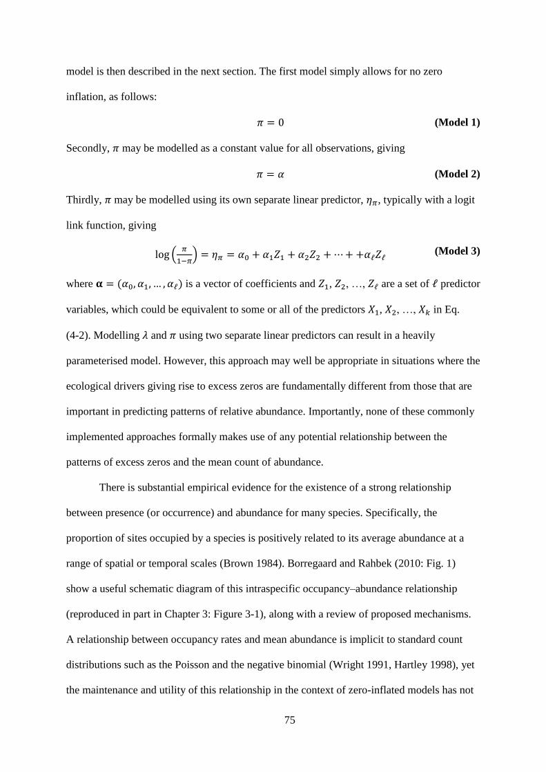
75
model is then described in the next section. The first model simply allows for no zero
inflation, as follows:
𝜋 = 0 (Model 1)
Secondly, 𝜋 may be modelled as a constant value for all observations, giving
𝜋 = 𝛼 (Model 2)
Thirdly, 𝜋 may be modelled using its own separate linear predictor, 𝜂𝜋, typically with a logit
link function, giving
log (𝜋
1−𝜋) = 𝜂𝜋 = 𝛼0 + 𝛼1𝑍1 + 𝛼2𝑍2 + ⋯ + +𝛼ℓ𝑍ℓ (Model 3)
where 𝛂 = (𝛼0, 𝛼1, … , 𝛼ℓ) is a vector of coefficients and 𝑍1, 𝑍2, …, 𝑍ℓ are a set of ℓ predictor
variables, which could be equivalent to some or all of the predictors 𝑋1, 𝑋2, …, 𝑋𝑘 in Eq.
(4-2). Modelling 𝜆 and 𝜋 using two separate linear predictors can result in a heavily
parameterised model. However, this approach may well be appropriate in situations where the
ecological drivers giving rise to excess zeros are fundamentally different from those that are
important in predicting patterns of relative abundance. Importantly, none of these commonly
implemented approaches formally makes use of any potential relationship between the
patterns of excess zeros and the mean count of abundance.
There is substantial empirical evidence for the existence of a strong relationship
between presence (or occurrence) and abundance for many species. Specifically, the
proportion of sites occupied by a species is positively related to its average abundance at a
range of spatial or temporal scales (Brown 1984). Borregaard and Rahbek (2010: Fig. 1)
show a useful schematic diagram of this intraspecific occupancy–abundance relationship
(reproduced in part in Chapter 3: Figure 3-1), along with a review of proposed mechanisms.
A relationship between occupancy rates and mean abundance is implicit to standard count
distributions such as the Poisson and the negative binomial (Wright 1991, Hartley 1998), yet
the maintenance and utility of this relationship in the context of zero-inflated models has not

76
been fully explored. Recently, two articles (Nielsen et al. 2005, Sileshi et al. 2009) have
examined the relationship between occupancy and abundance using parameters derived from
zero-inflated models with separate linear predictors for 𝜋. The results were mixed, indicating
that the relationship varies among taxa. For all five species of insect examined, parameters
for occupancy and abundance were strongly positively related (Sileshi et al. 2009), while for
moose, there was a weak positive relationship and, for bracken fern, there was no apparent
relationship (Nielsen et al. 2005). Although zero-inflated models have been used in the study
of occupancy–abundance relationships, this relationship, itself, has not yet been used
explicitly and directly to improve zero-inflated models. A model with a direct link between
zero inflation and abundance is presented in the next section.
4.3 The linked zero inflation model
Here, we suggest that an occupancy–abundance relationship can be incorporated
directly into a zero-inflated statistical model by using a very simple approach in which a
single linear predictor is used to model both 𝜋 and 𝜆 (Lambert 1992). The link between the
two parameters may be made by employing a simple linear model:
logit(𝜋) = 𝛾0 + 𝛾1𝜂𝜆 (Model 4)
where 𝜂𝜆 is the linear predictor for 𝜆 from Eq. (4-2) and 𝛾0 and 𝛾1 are parameters to be
estimated. The parameter 𝛾1 will usually be negative, reflecting a decreasing rate of zero
inflation (non-occupancy) with increasing 𝜆. Note that 𝜋 and 𝜆 are explicitly linked within the
modelling process, rather than examining the potential relationship post hoc, as in previous
studies (e.g., Nielsen et al. 2005, Sileshi et al. 2009).
The idea of linking 𝜋 and 𝜆 in zero-inflated models was originally proposed by
Lambert (1992) in the context of modelling defects in a manufacturing process. More
recently, Liu and Chan (2010, 2011) developed a library of functions for R (R Development
Core Team 2014), named COZIGAM, which can implement linked (“constrained”) zero-

77
inflated generalised additive models (GAMs). This general approach is not yet widespread,
however. Furthermore, COZIGAM is restricted to the one-parameter exponential family of
distributions (precluding, e.g., the negative binomial distribution) and can only implement
models that contain at least one nonparametric term, such as a smoothing function. Here, we
demonstrate that, within the Bayesian framework, the linked approach can be easily
implemented in a fully parametric model, incorporating generalized linear mixed model
structures with fixed and random factors and a nonstandard error distribution (i.e., the
negative binomial). These sorts of features are commonly required in ecological models.
In the following section, we present analyses of counts of snapper (Pagrus auratus:
Sparidae) from baited underwater video (BUV) deployments in north-eastern New Zealand.
We applied a set of potential models to allow for contagion and zero inflation in the four
forms just described. The linked model was found to give the best fit to the data with a
relatively modest number of parameters, and results obtained under this model are presented.
We then discuss in greater detail the advantages of using a zero-inflated mixture model that
directly links zero inflation with abundance in ecological studies.
4.4 Example
Background
This example uses data from a monitoring program of snapper (Pagrus auratus) at Te
Whanganui-A-Hei (Hahei) marine reserve, a no-take marine park covering 9 km2, established
in 1993 in north-eastern New Zealand (Willis et al. 2003a). This species is of considerable
ecological and commercial importance, and is the most heavily targeted recreationally fished
species in this region. Full details of the design of the monitoring program are provided in
Chapter 3: Section 3.4 and in Chapter 5: Section 5.3 (see also Willis et al. 2003a, Smith et al.
2014). The monitoring program consisted of BUV surveys (Willis and Babcock 2000), a

78
method which records video footage from a camera mounted on a steel frame, to which bait
is attached to attract carnivorous fish (see Chapter 3: Figure 3-2). The data here consisted of
counts of the maximum number of legal-sized (>27 cm fork length) individuals of snapper
seen in any single frame from each 30-min baited underwater video recording. This
standardized sampling unit ensured no individual fish was counted more than once (Willis et
al. 2003a), and was consistently applied across the entire study design. Here, the aim of the
analysis was to estimate the ratio of the density of legal-sized snapper in areas within the
reserve relative to areas outside of the reserve. The variation attributable to reserve status was
then compared to estimates of other spatial and temporal components of variation inherent in
the study design.
The monitoring program was designed as follows. A c. 10 km length of coast that
includes the reserve was divided into six areas: three within the reserve and three outside the
reserve (see Chapter 5: Figure 5-1, bottom-right panel). In a single survey, five (± 2) BUV
replicate drops were done at random locations within each area. Surveys were repeated in
each of nine years, specifically 1997–2001, 2003, 2004, 2006, and 2010. In each year,
surveys were done in spring (1997, 2004), autumn (1999, 2003, 2006, 2010), or both (1998,
2000, 2001), resulting in an unbalanced design. This yielded four factors in a hierarchical
mixed-effects ANOVA sampling design: reserve status (fixed), area (random, nested in
status), year (random), and season (fixed). There were 348 data values in total, 191 of which
were zeros.
Statistical methods
Data were analysed using a set of models with either Poisson or negative binomial
error distributions. Each of these base distributions was applied with each the following four
methods for zero inflation described in the previous sections, namely, no zero inflation

79
(model 1) constant zero inflation (model 2), zero inflation with its own separate linear
predictor (model 3), and the linked model (model 4). In addition, various combinations of the
four factors and their interactions (i.e., the predictor variables) were considered within each
class.
A Bayesian approach was used because of the relative ease with which complex
models can be fitted, including those with nonlinear and hierarchical model structures and
nonstandard (e.g., zero-inflated) error distributions, as required here. Parameter estimates
were obtained using Markov chain Monte Carlo (MCMC) methodology, implemented in the
software OpenBUGS (Lunn et al. 2009) and called from within R using the R2OpenBUGS
library (Sturtz et al. 2005). Standard noninformative prior distributions were used for all
estimated parameters (see Appendix A.1: Table A-1). Three MCMC chains were run for each
model and convergence was evaluated using the Brooks-Gelman-Rubin ��-statistic (Gelman
and Rubin 1992, Brooks and Gelman 1998). Each chain was run for a total of 750,000
iterations, of which a burn-in of 250,000 was excluded. The remaining 500,000 were thinned
at a rate of 1/50, providing three samples of 10,000 values that were combined for inferences.
The predictive performance of the models was compared using the Deviance
Information Criterion (DIC; Spiegelhalter et al. 2002) and a number of other measures of
performance and complexity. Some authors have suggested that the DIC is inappropriate for
mixture models when observation-level latent parameters are used in the likelihood function
(e.g. Lawson and Clark 2002). Here, a partially marginalised form of the likelihood was used,
thereby avoiding this problem (Millar 2009; see also Chapter 2). The summands of the DIC
were also used: the average deviance (��) provided an estimate of the overall goodness of fit
of the models to the data, while the effective number of parameters (𝑝𝐷) provided a measure
of model complexity. The latter was calculated as half the variance of the posterior deviance
(Gelman et al. 2014a), which is a less conventional alternative to the formulation proposed by

80
Spiegelhalter et al. (2002) with some important potential advantages (Link and Barker 2009).
The actual number of stochastic parameters (𝑝) was also noted. The remaining measures of
model fit were obtained from posterior predictive checks (Gelman et al. 2014a), using 5000
replicate data sets that were generated at random for each model with samples from the joint
posterior distributions of the parameters (𝑦𝑟𝑒𝑝). The 𝑦𝑟𝑒𝑝 were then compared with the
observed data (𝑦) on two summary statistics, namely the number of zero counts and the total
number of fish. Comparisons were made at two different levels, first by pooling at the level
of the whole data set (i.e., grand totals) and then at the level of the 72 bins of replicates as
delineated by the four factors of the study design (see Appendix A.1: Eqs. A-10 to A-13). A
full description of the finally selected model with further details of the calculations of derived
parameters, data and code, convergence diagnostics, posterior predictive checks, and
sensitivity analysis are provided in Appendix A.
Results
The DIC criterion favoured models based on the negative binomial distribution rather
than their Poisson-based counterparts, and using only the main effects as predictors for 𝜆.
Among these models, the lowest average deviance and the lowest DIC were obtained for
model 4, where 𝜋 was functionally linked to 𝜆 (Table 4-1). This model was also the most
accurate for predicting the number of zeros and also the total counts at either the level of the
entire data set or the level of the replicate bins. Despite requiring far fewer parameters, it
provided better predictions than even model 3.4, where all available factors were used to
predict 𝜆. Estimates for some key parameters obtained from model 4 are given below (see
Appendix A: Table A-2 for a more complete list). The shape of the relationship between 𝜋
and 𝜆 was negative (Figure 4-1). The posterior mean for the overall mean count of legal-sized

81
Tab
le 4
-1. A
com
par
ison
of
a se
lect
ion
of
candid
ate
model
s fo
r es
tim
atin
g t
he
counts
of
legal
ly s
ized
snap
per
fro
m a
mar
ine
rese
rve
monit
ori
ng
pro
gra
m. F
or
all
model
s sh
ow
n h
ere,
the
bas
e dis
trib
uti
on f
or
the
counts
was
the
neg
ativ
e bin
om
ial.
Four
clas
ses
of
zero
-infl
ated
model
s w
ere
use
d, as
indic
ated
by t
he
model
num
ber
s: (
1)
no z
ero i
nfl
atio
n, (2
) co
nst
ant
zero
infl
atio
n, (3
) a
sep
arat
e li
nea
r pre
dic
tor
for
zero
infl
atio
n, an
d
(4)
zero
infl
atio
n l
inked
to t
he
mea
n o
f th
e co
unt
pro
cess
. In
the
case
of
mo
del
3, su
bm
odel
s 3.1
–3.4
conta
in i
ncr
easi
ng n
um
ber
s of
par
amet
ers
in
the
separ
ate
linea
r p
redic
tor
for
zero
-infl
atio
n, as
indic
ated
. T
he
pre
dic
tor
var
iable
s ar
e den
ote
d a
s fo
llow
s: R
= r
eser
ve
stat
us;
S =
sea
son;
A =
area
; Y
= y
ear.
Model
s w
ere
com
par
ed u
sin
g t
he
Dev
iance
Info
rmat
ion C
rite
rion (
DIC
) an
d i
ts s
um
man
ds,
the
expec
ted d
evia
nce
(��
) an
d t
he
effe
ctiv
e num
ber
of
par
amet
ers
(𝑝𝐷
). T
he
actu
al n
um
ber
of
stoch
asti
c p
aram
eter
s (𝑝
) is
als
o p
rovid
ed.
The
mea
n o
f th
e post
erio
r pre
dic
tive
dis
trib
uti
ons
for
the
tota
l num
ber
of
zero
s (T
ota
l 𝑛
0) an
d t
he
tota
l co
unt
(Tota
l 𝑡)
is
pre
sente
d. T
hes
e m
ay b
e co
mpar
ed w
ith t
he
sam
e val
ues
from
the
obse
rved
dat
a, n
amel
y 1
91 a
nd 6
60, re
spec
tivel
y. F
inal
ly, es
tim
ates
of
the
mea
n a
bso
lute
err
or
for
each
of
𝑛0
and 𝑡
, poole
d a
t th
e le
vel
of
repli
cate
bin
s, p
rovid
e th
e “m
ean b
in m
iscl
assi
fica
tion r
ate”
(B
in 𝜖
��0)
and t
he
“mea
n b
in a
bso
lute
dev
iati
on”
(Bin
𝜖��).
For
thes
e m
easu
res,
smal
ler
val
ues
indic
ate
more
acc
ura
te p
redic
tions.
(S
ee A
ppen
dic
es A
.1 a
nd
A.6
for
furt
her
det
ails
of
the
model
and p
ost
erio
r pre
dic
tive
chec
ks.
)
Mo
del
D
evia
nce
and m
odel
com
ple
xit
y
Po
ster
ior
pre
dic
tive
chec
ks
Num
ber
M
od
el f
or
log(λ
) M
od
el f
or
logit
(π)
DIC
��
𝑝
𝐷
𝑝
Tota
l 𝑛
0
Tota
l 𝑡
Bin
𝜖��
0B
in 𝜖
��
1
R +
S +
A +
Y
0
1032.8
1012.7
20.1
21
18
0
70
9
0.8
9
5.5
2
R +
S +
A +
Y
𝛼
1030.2
1008.7
21.5
22
18
4
68
0
0.9
3
5.2
3.1
R
+ S
+ A
+ Y
R
1031.4
1005.1
26.3
23
18
6
67
9
0.9
1
5.1
3.2
R
+ S
+ A
+ Y
R
+ S
1031.8
1002.8
29.0
24
18
7
67
5
0.8
9
5.0
3.3
R
+ S
+ A
+ Y
R
+ S
+ A
1036.3
1004.3
32.0
31
18
6
67
9
0.8
9
5.0
3.4
R
+ S
+ A
+ Y
R
+ S
+ A
+ Y
1041.7
1003.9
37.8
41
18
6
67
9
0.8
7
5.0
4
R +
S +
A +
Y
γ 0 +
γ1lo
g(λ
) 1018.0
994.9
23.1
23
19
0
67
0
0.8
6
4.8

82
Figure 4-1. The relationship between the conditional mean count (λ) of snapper (per baited
underwater video deployment) and the probability of an excess zero (π) for legally sized
snapper from a marine reserve monitoring program. This relationship was estimated using a
Bayesian zero-inflated model (Appendix A.1) where π and λ were linked explicitly as logit(π)
= γ0 + γ1log(λ). The black line shows this function using point estimates for the parameters
of γ0 = 0.34 and γ1 = 1.60. The grey lines show this function using the paired values of these
parameters under MCMC within their joint 95% credible bounds.
snapper per BUV deployment inside the reserve (averaged across areas, seasons and years)
was 3.02, with a 95% central credible interval (CI) of 1.12–6.18. Outside the reserve, it was
0.20 (CI = 0.03–0.59). The reserve effect, calculated as the ratio of the mean count per BUV
deployment inside vs outside the reserve, was estimated to have a posterior median of 16.36
(CI = 4.10–90.00). A comparison of the components of variation showed that reserve status
had a far greater influence on counts of snapper than did season, year or area (Appendix A.1:
Table A-2). With zero inflation incorporated into the model, the degree of overdispersion was
moderate, with 𝛿 estimated to be 2.9 (CI = 1.5–5.0).

83
4.5 Discussion
The occupancy–abundance relationship in snapper
In the example just described, we considered several models for estimating counts of
legal-sized snapper inside vs. outside of a marine reserve. These models differed in the way
in which the probability of an excess zero, 𝜋, was structured. According to the DIC statistic,
the best model was obtained when 𝜋 was functionally linked to the conditional mean of the
count distribution, 𝜆. As expected, the relationship was negative (i.e., 𝛾1 < 0), indicating that
the zero inflation reflected a positive relationship between occupancy and abundance for this
species. Here, the specific relationship predicted 𝜋 to be quite high (> 0.5) when 𝜆 < 1.2,
reducing to just 0.2 when 𝜆 = 2.9 (Figure 4-1), indicating that excess zeros occurred primarily
where the mean count was low. The ecological interpretation of this relationship is not
straightforward, as it is unknown whether it resulted from small-scale behavioural processes,
large-scale population processes, or some mixture of the two. For example, high probability
of an excess zero could have arisen in areas of low density because fish were less likely to
discover or approach the bait. At a larger scale, fish might actively seek to school more
closely with other fish (creating less uniform and more clumped spatial distributions, and
hence more zero counts) when the overall numbers of fish in an area are low. Causal
mechanisms underlying observed occupancy-abundance relationships clearly require further
study.
Advantages of the linked model
The distribution of individuals of a given species in nature can arise from a variety of
interacting ecological processes which operate at numerous scales, including mortality,
recruitment, dispersal, habitat specificity, environmental constraints, and interactions with
other organisms. When a survey is done, a sampling process is superimposed onto this

84
distribution to produce data. It is generally intended that a statistical model should reflect, as
closely as possible, the underlying distribution and the sampling process that gave rise to the
data to which it is applied. When considering the structure of a zero-inflated model, if the
distribution of a species shows a strong relationship between occupancy and abundance at the
relevant sampling scale, then explicitly incorporating this relationship may provide a better
model which more accurately reflects the underlying patterns and processes. Such a model
should then be favoured over others by model selection criteria. If, on the other hand, the
patterns in occupancy are distinct from those of abundance, then an alternative model may be
more appropriate, either with constant 𝜋 in the case where the excess zeros are not related to
the predictor variables, or with a separate linear predictor for 𝜋 in the case where they are.
When appropriate, the linked model (model 4) has several important advantages over
the more commonly used alternatives (i.e., models 2 and 3). First is the principle of
parsimony: we should seek to implement a model that adequately explains the variation in the
data while using a minimal number of parameters. Although model 2 adds only one
parameter to the base model, a constant rate of zero inflation across the whole data set may be
overly simplistic in many situations. In contrast, using model 3 allows for a range of values of
𝜋 but will generally require the introduction of many more parameters. Exploiting the link
between occupancy and abundance can achieve the best of both worlds: 𝜋 can take a wide
range of values through the inclusion of just two extra parameters (𝛾0 and 𝛾1).
From a practical point of view, if primary interest lies in estimating the overall mean
(𝜇), modelling 𝜋 separately from 𝜆 complicates the interpretation of the model with respect to
𝜇. Because 𝜇 is a function of both 𝜋 and 𝜆, the overall effects of the predictor variables on 𝜇
are split between the two linear predictors. This can be considered an advantage in cases
where different processes affect 𝜋 and 𝜆 (Cunningham and Lindenmayer 2005). However, if
not, model 4 has the advantage that the linear predictor 𝜂𝜆 is used to predict both 𝜋 and 𝜆,

85
thereby simplifying the process of model selection and interpretation of the coefficients. The
coefficients may be compared directly to identify those with the greatest influence on count
values, as they are determined by both the mean of the count process and the excess zeros
simultaneously. Model 4 also provides estimates of 𝛾0 and 𝛾1, which can yield useful insights
regarding the shape of the relationship between zero inflation and abundance (see Appendix
A.3).
Although implementation of the linked model is straightforward under the Bayesian
paradigm (see Appendix A.4 to access R and BUGS code), this approach introduces a
complex nonlinear structure that is difficult to implement using frequentist methods.
Nonetheless, there are important potential computational advantages to the linked model.
Where occupancy is strongly related to abundance, having separate predictors in the model is
likely to result in correlations among the two sets of coefficients. Intuitively, it is best to
avoid this sort of redundancy in the parameters of a model. Practically, correlated parameters
can result in problems with convergence and poor estimation when fitting the model. This
was apparent in our analysis when the MCMC chains for class-3 models generally took
longer to converge and had greater autocorrelation than the other models. Another
consideration is that, as 𝜋 approaches either 0 or 1, the data in its binary (i.e., observed or not
observed) form has low variance and contains very little information. This can cause low
statistical power and computational difficulties associated with extremely low (or high)
values on the logit scale, because as 𝜋 tends to 0 (or 1), logit(𝜋) tends to –∞ (or ∞)
(Cunningham and Lindenmayer 2005). The linked model may help relieve this problem
because the parameter estimates are determined by the full range of integer values in the data.
Here, we considered only the mixture-model approach to zero inflation, rather than
the hurdle approach where the count distribution is truncated so that it cannot produce zeros.
Although the mixture and hurdle models might give similar results, particularly if the mean

86
abundance is high (Welsh et al. 1996, Wenger and Freeman 2008), it can be argued that
truncating the count-generating distribution in this way is somewhat “artificial”. There may
be some practical advantages to eliminating zeros from the count model, such as
orthogonality of the two distributions (Welsh et al. 1996, Cunningham and Lindenmayer
2005), but it is difficult to justify why zeros should be precluded from occurring in any
stochastic ecological sampling process that produces counts of organisms. An ecological
sampling process, even in the absence of excess zeros, could easily generate a zero if the
mean is sufficiently low and/or the variance is sufficiently high. Furthermore, the mixture-
model approach has the advantage of operating with conventional, parametric distributions.
Another advantage of the zero-inflated mixture model is that it can provide direct
insights into the nature of the occupancy–abundance relationship for excess zeros. Under
standard count distributions, such as the Poisson or negative binomial, the rate of occupancy
is a fixed positive function of the mean abundance (𝜆) and, potentially, a dispersion
parameter. Under a zero-inflated mixture model, a zero can arise from either the base count
distribution (base zeros) or from the component of the model that allows for zero inflation
(excess zeros). The base zeros will follow the occupancy–abundance relationship implicit in
the base distribution. On the other hand, excess zeros may or may not be related to
abundance, depending in part on the structure of the model for zero inflation. For the models
described herein, model 2 asserts no relationship between excess zeros and abundance, and
model 3 assumes no structural relationship, although one might be produced indirectly. Only
model 4 directly relates excess zeros to the conditional mean abundance (𝜆). This
parsimonious method allows for the excess zeros to follow a similar relationship with
abundance to that of the base zeros. It also has the flexibility to allow for alternative forms of
the relationship, if so required (Appendix A.3).

87
4.6 Conclusion
Many authors (e.g., Martin et al. 2005, Potts and Elith 2006) have stressed that failure
to account for overdispersion and zero inflation in a statistical model can result in inaccurate
point or interval estimation of parameters, which may then lead to spurious conclusions.
Therefore, it is wise to put some effort into considering alternative model structures when
standard models fail to provide an adequate representation of distribution of the data. For
models that require zero inflation, the general approach of modelling the probability of an
excess zero as a function of the conditional mean of the count values may be used to great
advantage in cases where they are indeed related. Clearly, if no such relationship is present,
other models for 𝜋 should be considered instead. The general linear structure for the link
between 𝜋 and 𝜆 proposed here can produce a wide variety of useful relationships (Appendix
A.3). Nevertheless, we encourage further research to evaluate alternative forms of this
relationship in predictive models for real data, including alternative link functions for binary
data (such as the complementary log-log or probit functions) and other forms of linkage
suggested by empirical analyses of the occupancy–abundance relationship (He and Gaston
2003, Sileshi et al. 2009; see also Appendix A.7).We conclude that the incorporation of
occupancy– abundance relationships into models of zero inflation provides a key tool to
develop more accurate and parsimonious models of ecological count data.
4.7 Acknowledgements
I thank the Department of Conservation (DOC Inv 4238) and Massey University
(specifically the Institute for Information and Mathematical Sciences and the New Zealand
Institute for Advanced Study) for financial and logistic support. I also thank Trevor Willis
and DOC for the provision of data. I thank my co-authors Marti Anderson and Russell Millar
for their contribution to the published article in Ecology. The article was also improved by

88
comments from handling editor Brian Inouye an anonymous reviewer, Seth Wenger, and
Robert Dorazio.

89
Chapter 5. Effects of marine reserves in the context of
spatial and temporal variation: an analysis using Bayesian
zero-inflated mixed models
This chapter was published in
Smith, A. N. H., M. J. Anderson, R. B. Millar, and T. J. Willis. 2014. Marine Ecology
Progress Series 499:203–216.
5.1 Abstract
Evaluating the effects of marine reserves on exploited species can be challenging
because they occur within a context of natural spatial and temporal variation at many scales.
For rigorous inferences to be made, such evaluations require monitoring programmes that are
replicated at appropriate scales. We analysed monitoring data of snapper Pagrus auratus
(Sparidae) in north-eastern New Zealand, comprised of counts from baited-underwater-video
surveys from inside and outside three marine reserves. Surveys were replicated at many
levels, including areas inside and outside of marine reserves at three locations in two seasons,
over a period of up to 14 years, in an unbalanced design. The Bayesian modelling approach
allowed the use of some familiar aspects of ANOVA, including mixed models of fixed and
random effects, hierarchically nested structures, and variance decomposition, while allowing
for overdispersion and excess zeros in the counts. Model selection and estimates of variance
components revealed that protection by marine reserves was by far the strongest measured
source of variation for relative densities of legal-sized snapper. The size of the effect varied
across years among the three reserves, with relative densities between 7 and 20 times greater
in reserves than in nearby areas. Other than the reserve effect, the temporal factors of season
and year were generally more important than the spatial factors at explaining variation in
counts. In particular, overall relative densities were ~2 to 3 times greater in autumn than in

90
spring for legal-sized snapper, although the seasonal effect was also variable among locations
and years. We consider that the Bayesian generalised linear mixed modelling approach, as
used here, provides an extremely useful and flexible tool for estimating the effects of
management actions and comparing them directly with other sources of spatial and temporal
variation in natural systems.
5.2 Introduction
The exploitation of marine species by humans has caused the depletion of many
stocks of fishes worldwide (Pauly et al. 2005, Worm and Branch 2012). No-take marine
reserves, designated areas in which all harvesting and damaging of marine life is prohibited
(Lubchenco et al. 2003), are increasingly being used as part of the effort to ameliorate this
trend. If sufficiently enforced, marine reserves have been shown to increase the size and
abundance of exploited species within their borders (Mosquera et al. 2000, Micheli et al.
2004, Claudet et al. 2010, Babcock et al. 2010). This, in turn, may produce secondary
ecological effects, such as enhancing populations of exploited species beyond the boundaries
of the reserve (Roberts and Polunin 1991, Dugan and Davis 1993, Stoner and Ray 1996,
Bohnsack 1998) or facilitating changes in habitat through trophic cascades (Babcock et al.
1999, Salomon et al. 2008, Leleu et al. 2012). The value of marine reserves is primarily as a
means to manage and protect exploited or endangered species in a particular area, which may
then produce broader benefits in terms of increased biodiversity and ecosystem function.
For marine reserves to be used effectively as a management tool, it is critical to be
able to estimate and predict their effects. Studies that monitor the abundance of exploited
species in existing marine reserves are an essential source of information on which to base
such predictions. Accurately quantifying the effects of marine reserves on exploited species
can be challenging, however. Data from such studies, often in the form of counts, can be
overdispersed or contain excess zeros (Chapter 4; Smith et al. 2012), requiring statistical

91
models to be based on nonstandard distributions. Furthermore, marine ecosystems exhibit
considerable variation at several temporal and spatial scales (Underwood et al. 2000).
Hierarchical sampling regimes that span these scales of variation are therefore necessary to
obtain rigorous estimates of the effects of reserves (Andrew and Mapstone 1987, García-
Charton and Ruzafa 1999, García-Charton et al. 2000, Willis et al. 2003b). For example, if
the abundance of an organism varies from year to year, then a study that spans several years
will enable far more accurate estimates of long-term effects as well as provide information on
inter-annual variation. The extent to which abundance varies in time and space at different
scales is interesting in itself and provides a context of the underlying ‘natural’ variation with
which to compare any measured effect of marine reserves. While some authors have stressed
the need to make such comparisons (García-Charton and Ruzafa 1999, García-Charton et al.
2000, 2004), appropriate statistical methods for directly comparing sources of variation in
studies of reserve effects have not been explicitly specified.
Here, we analyse a long-term, spatially replicated monitoring dataset of counts of
snapper Pagrus auratus (Sparidae) from areas inside and outside each of three marine
reserves in north-eastern New Zealand. The analysis used a Bayesian approach outlined by
Gelman (2005) for ANOVA, which was extended here to more complex zero-inflated
generalised linear mixed models (GLMMs). This approach easily incorporated the
unbalanced hierarchical structure of the study design in combination with nonstandard error
distributions to allow for overdispersion and excess zeros. The primary aim was to estimate
the effects of marine reserve protection on counts of snapper while simultaneously
accounting for other sources of variation at various spatial and temporal scales. We then
compared the estimated reserve effects with other sources of variation in the study design
using variance components. The consistency of reserve effects in time and space was also
evaluated by estimating interactions between the reserve effect and other factors.

92
5.3 Materials and methods
Background and sampling design
Snapper is an important coastal species in temperate north-eastern New Zealand,
supporting the country’s largest inshore commercial and recreational fisheries (Maunder and
Starr 2001). Stocks of snapper in this region (fisheries management area known as SNA1) are
believed to be slowly rebuilding since being heavily exploited and reduced below the
maximum sustainable yield in the latter half of the 20th century (Ministry for Primary
Industries 2013). Snapper is also ecologically important, with strong evidence that its
predation of sea urchins Evechinus chloroticus can contribute to a trophic cascade that allows
the restoration of kelp Ecklonia radiata forests within marine reserves in some contexts
(Babcock et al. 1999, Shears et al. 2008). There is also some evidence that small crypto-
benthic fishes may be affected by large densities of snapper in a marine reserve (Willis and
Anderson 2003).
An ongoing monitoring programme of the relative density of snapper in areas inside
and outside (adjacent to) marine reserves at three locations in the north-eastern bioregion of
New Zealand, namely Leigh, Tāwharanui, and Hahei (Table 5-1, Figure 5-1), began in 1997.
These three locations have broadly similar habitat and environmental conditions (Shears et al.
2008). Refer to Willis, Millar, & Babcock (2003a) for a description and analysis of the first
three years of data and Drake (2006) for preliminary Bayesian modelling of the data from
Leigh only. The programme used a baited-underwater-video (BUV) sampling method (Willis
and Babcock 2000), which was developed following reports that snapper were differentially
attracted to divers within reserves compared to outside reserves, thereby introducing bias into
the usual underwater-visual-survey method (Cole 1994). The data are in the form of counts,
taken as the maximum number of snapper seen in any one frame of a 30 min long underwater
video deployment (‘MaxN’). This is assumed here to be a measure of the relative density of

93
Table 5-1. Details regarding the age and size of each of the three marine reserves examined
in this study.
Marine reserve
Year
established
Area
(ha)
Approx.
coastal
extent (m)
Approx.
offshore
extent (m)
Cape Rodney-Okakari Point (Leigh) 19771 518 5,240 800
Tāwharanui 1981 350 3,200 800
Te Whanganui-A-Hei (Hahei) 1992 840 3,740 1,850
1Note that some sources have given the date of establishment for this reserve as 1975. In their
original description of the reserve, Ballantine and Gordon (1979) indicate that it was legally
established in 1975, but was officially opened and became operational in 1977.
Table 5-2. The number of baited underwater video (BUV) sampling units obtained in each
year, season and location. Samples within each survey were allocated to reserve and non-
reserve areas equally in most cases.
Leigh Tāwharanui Hahei
Year Autumn Spring Autumn Spring Autumn Spring
1997 - 48 - 24 - 27
1998 48 48 24 24 30 25
1999 48 - 24 - 30 -
2000 47 43 - - 30 30
2001 48 47 - - 26 30
2002 48 - - - - -
2003 48 - - - 30 -
2004 - - - - - 30
2005 48 - - - - -
2006 - - - - 30 -
2007 48 - 32 - - -
2010 - - - - 30 -

94
Figure 5-1. A map showing the locations of three marine reserves in north-eastern New
Zealand (upper left panel). Also shown are the individual numbered areas (fine lines and
numbers), and marine reserves (bold lines) at each location, as indicated. Note that the
borders of Tāwharanui Marine Reserve were moved slightly in September 2011 and are now
different to those shown here.
snapper. Snapper were divided into those below (‘sublegal’) and above (‘legal’) the
recreational minimum legal size of 27 cm fork length (scheduled to increase to 30 cm in April
2014), and these two size classes were modelled separately.
At each of the three locations, the coastline was divided into several areas, some
falling inside and some falling outside the marine reserves (Figure 5-1). Note that at each
location, the areas falling outside of the reserve occurred in both directions along the
coastline to avoid spatial confounding of areas with reserve effects. Monitoring surveys
began in 1997 and were carried out twice per year in each of two seasons, spring (primarily
September to December) and autumn (primarily March to June), but surveys were not
repeated consistently at all locations after the autumn survey of 1999, yielding an overall
95
sampling design that is highly unbalanced in its cell structure (Table 5-2). The two seasons
were included in the monitoring design because some individuals of this species undergo a
seasonal inshore migration which causes inshore densities to increase during summer months
and subsequently decline during winter months (Willis et al. 2003a, Willis and Millar 2005).
At the time of each survey at a particular location, n = 3 to 6 (usually 4) replicate BUV
deployments were done at haphazardly chosen positions within each area. A total of n = 1045
deployments were included in the models described here (Table 5-2). This sampling design
yielded five factors: Reserve (fixed with two levels, inside and outside), Season (fixed with
two levels, autumn and spring), Year (random with up to 12 levels), Location (fixed with
three levels), and Area (random, nested in Reserve × Location, with up to 6 levels per
combination of reserve and location; see Figure 5-1). We chose to treat Location as a fixed
effect because the focus was to estimate the effects for these particular reserves rather than
for reserves in general.
Candidate models and model selection
Counts of sublegal and legal snapper from the monitoring programme were analysed
using Bayesian zero-inflated GLMMs. Following Gelman (2005), we used the Bayesian
approach to model variation associated with the effects of marine reserves, as well as seasons,
locations, areas, and years, in a structured ANOVA framework. The term ANOVA is used
here to refer specifically to the structuring of the coefficients into ‘batches’, so that the levels
of each categorical factor are grouped together. Variance components are estimated for each
batch of coefficients to compare the relative importance of the terms in the model. In our
models, Gelman’s (2005) framework was extended to include error structures considerably
more complex than those of traditional Gaussian ANOVA, as required to account for over -
dispersion and zero inflation.

96
Models were implemented using Markov chain Monte Carlo (MCMC) methodology
with the software OpenBUGS (Lunn et al. 2009), called from within R (R Development Core
Team 2014) by the R2OpenBUGS library (Sturtz et al. 2005). Each model was run with three
chains, each having a length of 100,000 iterations, from which a burn-in of 50,000 was
discarded. The chains were thinned at a rate of 1 in 5, resulting in a total of 30,000 values
being kept for each model. Convergence was checked using the Brooks-Gelman-Rubin ��-
statistic (Gelman and Rubin 1992, Brooks and Gelman 1998).
The full five-factor experimental design, including all of the potential interactions
among factors, was highly complex, having a total of 19 terms (Table 5-3). Because of the
number of missing cells in the sampling design (Table 5-2), leading to non-identifiability,
heuristics were used first to identify appropriate candidate predictor terms for model
selection. Specifically, candidate terms for model selection did not include interactions higher
than third order and also did not include the third-order interaction that did not involve
Reserves (i.e. Season × Year × Location; see Table 5-3). A formal model-selection procedure
was then used to choose the most favourable model out of hundreds of remaining available
candidate models for each of the sublegal- and legal-sized snapper datasets.
The candidate models differed in two key respects: the structure of the distribution of
errors and the factors (including interactions) that were included. The base distributions
considered for the errors were the zero-inflated Poisson (ZIP) and the zero-inflated negative
binomial (ZINB). Both the ZIP and the ZINB had the parameters 𝜆, the mean of the Poisson
distribution conditional on the absence of excess zero, and 𝜋, the probability of the
occurrence of an excess zero. In addition, the ZINB had the parameter 𝛿, which allowed for
aggregation (overdispersion) in the counts. For either of these error distributions, the overall
mean is given by
𝜇 = (1 − 𝜋)𝜆 (5-1)

97
Table 5-3. Sources of variation for the full ANOVA model, based all factors in the study
design. The terms that were not included as candidates for model selection, based on
preliminary heuristics, are indicated with an asterisk. The abbreviation for each term, as
shown, was used to indicate the model parameters associated with that term in the GLMs,
given in Equations (5-3) to (5-5) in the text. Terms that were chosen to be included in the
final models of relative densities of legal or sublegal snapper, obtained using model selection
on the basis of the DIC, are also provided.
Source of variation Abbreviation Degrees
of
Freedom
Fixed or
random
Selected for
sublegal (S)
or legal (L)
models
Reserve R 1 Fixed L
Season S 1 Fixed S L
Location L 2 Fixed S L
Year Y 11 Random S L
Area (nested in L×R) A 20 Random S L
Reserve×Season RS 1 Fixed
Reserve×Location RL 2 Fixed L
Reserve×Year RY 11 Random L
Season×Location SL 2 Fixed S L
Season×Year SY 2 Random S L
Season×Area (nested in L×R) SA 18 Random
Location×Year LY 8 Random S
Year×Area (nested in L×R) YA 124 Random
Reserve×Season×Location RSL 2 Fixed
Reserve×Season×Year RSY 2 Random
Reserve×Location×Year RLY 8 Random
Season×Location×Year* SLY 8 Random
Season×Year×Area (nested in L×R)* SYA 28 Random
Reserve×Season×Year×Location* RSYL 2 Random

98
The conditional mean, 𝜆, was modelled as a linear predictor of candidate terms with a
log-link function. Zero inflation, 𝜋, was incorporated using one of four alternative types of
models (Chapter 4; Smith et al. 2012): (1) no zero inflation (𝜋 = 0); (2) constant zero
inflation (𝜋 = 𝛼, where 𝛼 is a single constant parameter to be estimated); (3) zero inflation
linked to the conditional mean (Chapter 4; Smith et al. 2012); and (4) zero inflation modelled
as a separate linear predictor of the candidate terms with a logit-link function. A computing
cluster with multiple processors allowed us to conduct a thorough search for the best
combination of terms (including two- and three-way interactions; see Table 5-3) for
modelling 𝜆, and also 𝜋 in the case of zero inflation by way of a separate model (type 4
above). The general approach began by fitting the most complex model with the full set of
candidate terms (as listed in Table 5-3). A batch of models was then run, where each model
had one of the poorest-performing terms removed, and then the process was repeated. Third-
order interactions were removed prior to second-order interactions, in a logical sequence, and
no models included interaction terms involving main effects that were not also included in the
candidate model. This approach for selecting appropriate terms was done separately for both
types of error distributions and for all four types of zero-inflated models for estimating 𝜋.
Model selection was based on the deviance information criterion (DIC; Spiegelhalter et al.
2002, Millar 2009), using half the variance of the posterior deviance for estimating the
effective number of parameters, 𝑝𝐷 (Link and Barker 2009, Gelman et al. 2014a). Some
models were excluded because of very high variance in the posterior distributions of some
parameters, which was probably caused by poor identifiability (Omlin and Reichert 1999).
The final models chosen, from those that remained, were those with the fewest parameters
within two units of the lowest DIC score.

99
Structure of the selected models
For both sublegal- and legal-sized snapper, the count (𝑦) in replicate m in Year 𝑙,
Area 𝑘 (nested in Reserve × Location), Location 𝑗, Season 𝑖, and Reserve status ℎ was best
modelled using the negative binomial distribution
𝑦ℎ𝑖𝑗𝑘𝑙𝑚 ~ ZINB(𝜆ℎ𝑖𝑗𝑘𝑙, 𝜋ℎ𝑖𝑗𝑘𝑙 , 𝛿) (5-2)
For sublegal-sized snapper, the linear predictor for the conditional mean 𝜆 was
log(𝜆ℎ𝑖𝑗𝑘𝑙) = 𝛽0 + 𝑆𝑖 + 𝐿𝑗 + 𝐴𝑘(𝑗) + 𝑌𝑙 + (𝑆𝐿)𝑖𝑗 + (𝑆𝑌)𝑖𝑙 + (𝐿𝑌)𝑗𝑙 (5-3)
and excess zeros required the use of a separate linear predictor (type 4), namely
log (
𝜋ℎ𝑖𝑗𝑘𝑙
1 − 𝜋ℎ𝑖𝑗𝑘𝑙) = 𝛽0
(𝜋)+ 𝐿𝑗
(𝜋)+ 𝐴𝑘(𝑗)
(𝜋) (5-4)
For legal-sized snapper, the linear predictor for 𝜆 was
log(𝜆ℎ𝑖𝑗𝑘𝑙) = 𝛽0 + 𝑅ℎ + 𝑆𝑖 + 𝐿𝑗 + 𝐴𝑘(𝑗) + 𝑌𝑙 + (𝑅𝐿)ℎ𝑗 + (𝑅𝑌)ℎ𝑙
+ (𝑆𝐿)𝑖𝑗 + (𝑆𝑌)𝑖𝑙
(5-5)
and the model for the zero inflation parameter was
log (
𝜋ℎ𝑖𝑗𝑘𝑙
1 − 𝜋ℎ𝑖𝑗𝑘𝑙) = 𝛾0 + 𝛾1 log(𝜆ℎ𝑖𝑗𝑘𝑙) (5-6)
using Smith et al.’s (2012) ‘linked’ model (see also Chapter 4), where the logit of the zero
inflation parameter was modelled as a linear function of the log of the conditional mean
count, using the parameters 𝛾0 and 𝛾1 which were estimated (Type 3). In Equations (5-3) to
(5-5), 𝛽0 is an overall fitted mean, and the subsequent abbreviations correspond to parameters
for individual terms in the model, as indicated in Table 5-3. Within each factor, the
coefficients were centred on zero (see Equation 5-9), so that estimates of mean counts of
interest (e.g. the overall mean within reserves) could be constructed based on the above
equations, where the values of 𝜆 and 𝜋 are obtained by adding the appropriate estimates of

100
coefficients to the global mean and back-transforming through the above equations. For
example, the overall mean inside reserves 𝜇𝑅 for legal snapper was calculated as
𝜇𝑅 = (1 −
1
1 + 𝑒−(𝛾0+𝛾1 log 𝜆𝑅)) × 𝜆𝑅 (5-7)
where the conditional mean count within reserves is 𝜆𝑅 = 𝑒𝛽0+𝑅𝑟𝑒𝑠𝑒𝑟𝑣𝑒 .
Parameterisation and prior distributions for model terms
Let 𝐴 be a factor represented by a vector of coefficients 𝛃 = (𝛽1, … , 𝛽ℓ), where ℓ is
the number of levels in 𝐴. If the factor 𝐴 was fixed, coefficients 𝛽1 to 𝛽ℓ−1 were each given
prior distributions
𝛽 ~ Norm(0, 100) (5-8)
A sum-to-zero constraint was used for fixed factors, such that one coefficient was set to
𝛽ℓ = − ∑ 𝛽𝑎
ℓ−1
𝑎=1
(5-9)
For interactions between fixed and random factors, this constraint was also used for the fixed
factor within each level of the random factor. Components of variation for fixed factors were
defined as
𝜎𝐴
2 =∑ 𝛽𝑎
2ℓ𝑎=1
ℓ − 1 (5-10)
We refer to these as ‘variance components’ in the following, although for fixed factors these
are, strictly speaking, not variances but sums of squared fixed effects divided by the
appropriate degrees of freedom.
If 𝐴 was a random factor, the coefficients were given prior distributions
𝛽 ~ Norm(0, 𝜎𝐴2) (5-11)
where 𝜎𝐴2 is common to all coefficients and represents the variance component for factor 𝐴.
The square roots of variance components for random factors were given standard half-

101
Cauchy priors (Gelman 2006). The dispersion parameter for models with the ZINB
distribution was given the prior distribution of
𝛿 ~ Gamma(0.0001, 0.0001) (5-12)
For type-3 zero-inflated models, the parameters 𝛾0 and 𝛾1 were both given the prior
distribution of
𝛾0, 𝛾1 ~ Unif(−5, 5) (5-13)
Code for fitting the selected models for both sublegal- and legal-sized snapper in R and
OpenBUGS is provided in Appendix B.
5.4 Results
Spatial factors: effect of reserve status and variation among locations and areas
For legal snapper, reserve status was by far the greatest source of variation (Figure
5-2). After controlling for variation among locations, areas, seasons, and years, the overall
reserve effect (i.e. the ratio of mean MaxN counts in reserve vs. non-reserve areas) was
estimated to be 13.4 (see Table 5-4 for credible intervals). However, the reserve effect
differed substantially among locations, as evidenced by inclusion of the Reserve × Location
interaction term in the model, with the greatest effect observed at Leigh (effect size of 19.3),
followed by Hahei (16.0) and then Tāwharanui (7.8). Estimated mean MaxN counts per BUV
deployment (mean relative densities) in non-reserve areas were around 0.4 for both Leigh and
Tāwharanui and 0.2 for Hahei. In protected areas, Leigh had by far the greatest mean relative
density at 7.5, compared to ~3 in Tāwharanui and Hahei. In contrast, for sublegal snapper,
reserve status was not included in the chosen model at all. Instead, the two spatial factors
(Location and Area) were most important for determining the occurrence of excess zeros in
sublegal snapper, with the smaller scale of areas being most important (Figure 5-2). For

102
Table 5-4. Point estimates (mean of the posterior distribution, represented by the set of
values given by MCMC) and 95% credible intervals (0.025 and 0.975 quantiles of the
posterior distribution) of the mean relative densities for either sublegal or legal snapper in
reserve and non-reserve areas at each of three locations. Reserve and non-reserve densities
for sublegal snapper were pooled because there was no reserve effect in the model. Estimates
of the ratio of reserve to non-reserve densities are also provided for legal snapper as an index
of the ‘reserve effect’. The point estimates for the ratios were obtained by first calculating the
ratios for each MCMC iteration, taking the natural log of the ratios, calculating the mean, and
then back-transforming.
Sublegal Legal
Location Non-reserve
and Reserve
Non-reserve Reserve Ratio R:NR
Leigh 3.08
(1.97, 4.46)
0.40
(0.17, 0.74)
7.49
(4.42, 12.09)
19.34
(8.76, 44.18)
Tāwharanui 3.34
(1.81, 5.63)
0.41
(0.15, 0.84)
3.05
(1.40, 5.48)
7.77
(2.98, 22.06)
Hahei 1.79
(0.97, 2.88)
0.19
(0.06, 0.42)
2.89
(1.26, 5.48)
16.02
(5.37, 50.76)
All reserves 2.67
(1.8, 3.73)
0.30
(0.15, 0.50)
3.98
(2.49, 5.92)
13.43
(7.43, 25.48)
predicting the conditional mean counts of sublegal snapper, temporal factors were most
important, especially year. Densities of sublegal fish varied among locations, however, with
Leigh and Tāwharanui supporting densities ~1.5 times that of Hahei (Table 5-4).
At the finer spatial scale of areas, mean relative densities of sublegal snapper were
similar inside and outside reserves (Figure 5-3). Credible intervals around the estimated
means of areas were too large to make strong conclusions about fine-scale spatial patterns.
However, there was potentially a gradient of increasing density from the westernmost area
(Area 1) to Cape Rodney (Areas 9 and 10). At Tāwharanui, there was little variation in
estimated mean densities of sublegal snapper among areas. At Hahei, the highest estimated
mean density of sublegal snapper was from the central area of the reserve. For legal snapper,

103
Figure 5-2. A variance components plot (Gelman 2005) showing the variation associated
with each term in the chosen models, expressed as the estimate of the standard deviation σ
among levels, for predicting the relative density of legal or sublegal snapper. For the latter,
separate linear predictors were used to model the probability of an excess zero (π) and the
conditional mean of the counts (λ), so a separate panel is used for each. Point estimates
(means of posterior distributions) are represented by vertical lines, with 50% and 95%
credible intervals for the means as thick and thin horizontal lines, respectively.

104
relative densities were consistently very low outside of the reserves at all locations, and there
was no apparent trend with proximity to the reserve. The greatest densities of legal snapper
were found in the central areas of the reserve at Leigh (Areas 5 and 6), with densities
declining steeply towards the eastern and western boundaries of the reserve. Within the
reserves at Tāwharanui and Hahei, however, there were gradients of increasing density from
east to west and west to east, respectively. There did not appear to be any consistent
relationship between the densities of sublegal and legal snapper among areas, except perhaps
in non-reserve areas at Leigh, where similar spatial patterns were apparent for the two size
classes.
Regarding causal inferences, we note that the marine reserves in the present study
were established long before this monitoring programme began, so a before-after-control-
impact (BACI) type design (Underwood 1991), which would have provided stronger
evidence for the causal effects of the establishment of the marine reserves, was not possible.
Thus, the estimated reserve effects might be due to differences in the habitat or environment
between the existing designated reserve and non-reserve areas. However, our general
conclusion that the differences observed were caused by the absence of fishing in the reserves
is supported by the fact that strong effects for legal-sized snapper occurred in all three marine
reserves, there was no spatial pseudoreplication of the areas sampled at any of these
locations, and no such reserve effects were observed for sublegal-sized snapper.
Temporal factors: seasonal effects and variation among years
Mean counts of sublegal- and legal-sized snapper were greater in autumn than in
spring (Table 5-5). The effect was strong for legal snapper and was the second most
important source of variation (Figure 5-2), with an estimated seasonal effect size (ratio of
densities in autumn vs. spring) of 2.6. The overall effect was less convincing for sublegal
snapper, with an estimated effect size of 1.8 and a 95% credible interval that included 1. The

105
Table 5-5. Point estimates and 95% credible intervals (as described in the legend for Table
5-4) of the mean relative densities for either legal or sublegal snapper in each of two seasons
at each of three locations. Estimates for ratios of seasonal effects were obtained as described
for reserve effects in the caption for Table 5-4.
Estimates
Size class Location Spring Autumn Ratio A:S
Sub-legal Leigh 2.49
(1.38, 3.99)
4.48
(2.67, 6.69)
1.81
(0.99, 3.16)
Tāwharanui 2.91
(1.12, 5.9)
3.06
(1.68, 5.37)
1.11
(0.49, 2.44)
Hahei 1.18
(0.62, 2.01)
3.45
(2.05, 5.25)
2.97
(1.62, 5.35)
All reserves 1.96
(0.97, 3.27)
3.37
(2.18, 4.94)
1.76
(0.98, 3.12)
Legal Leigh 1.35
(0.67, 2.34)
2.65
(1.56, 4.08)
2.01
(1.07, 3.96)
Tāwharanui 0.73
(0.28, 1.41)
1.8
(0.91, 3.09)
2.54
(1.16, 6.1)
Hahei 0.43
(0.16, 0.85)
1.39
(0.71, 2.37)
3.35
(1.67, 7.33)
All reserves 0.74
(0.37, 1.24)
1.86
(1.14, 2.74)
2.55
(1.35, 5.15)
models selected for both size classes included interaction terms, indicating that the effect of
season differed among years and locations (Table 5-3). For both size classes, the seasonal
effect was greater for Hahei than at other locations, driven by relatively low densities in
spring. There was little evidence of a strong seasonal effect on sublegal fish at Tāwharanui,
but there was only one year in which this location was surveyed in both seasons.
Annual variation was also important for both size classes (Figure 5-2), with mean
relative densities varying substantially among the 12 years of the study (Figure 5-4). The
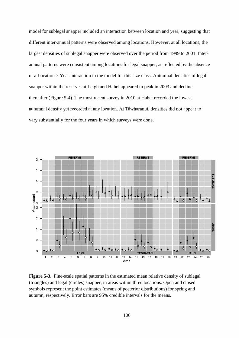
106
model for sublegal snapper included an interaction between location and year, suggesting that
different inter-annual patterns were observed among locations. However, at all locations, the
largest densities of sublegal snapper were observed over the period from 1999 to 2001. Inter-
annual patterns were consistent among locations for legal snapper, as reflected by the absence
of a Location × Year interaction in the model for this size class. Autumnal densities of legal
snapper within the reserves at Leigh and Hahei appeared to peak in 2003 and decline
thereafter (Figure 5-4). The most recent survey in 2010 at Hahei recorded the lowest
autumnal density yet recorded at any location. At Tāwharanui, densities did not appear to
vary substantially for the four years in which surveys were done.
Figure 5-3. Fine-scale spatial patterns in the estimated mean relative density of sublegal
(triangles) and legal (circles) snapper, in areas within three locations. Open and closed
symbols represent the point estimates (means of posterior distributions) for spring and
autumn, respectively. Error bars are 95% credible intervals for the means.

107
Figure 5-4. Inter-annual and season patterns in the estimated mean relative density of
sublegal (triangles) and legal (circles) snapper at three locations. Open and closed symbols
represent the point estimates (means of posterior distributions) for spring and autumn,
respectively. Error bars are 95% credible intervals for the means. For legal snapper, estimates
for within the reserves only are shown, because too few snapper were observed outside the
reserves to show any interpretable patterns. Note that the scale of the y-axes varies differ for
sublegal (left) and legal (right) panels.

108
5.5 Discussion
Effects of protection by marine reserves on snapper
Marine reserve protection was by far the most important determinant of the relative
density of legal snapper, with the estimated component of variation associated with the
reserve effect being much greater than any of the other spatial or temporal factors (Figure
5-2). When averaged across all other factors, the relative density of legal snapper was
estimated to be 13 times greater inside reserves than outside reserves (Table 5-4), a result
similar to the value of 14 times greater, which was reported from an analysis of the first three
years of this monitoring program (Willis et al. 2003a).
Our results indicated large differences in the effects of reserves on legal snapper
among locations, which were not reported by Willis, Millar, & Babcock (2003a). Differences
in reserve effects have also been observed in a recent study of another species (rock lobster
Jasus edwardsii) in a set of reserves which included the three studied here (Freeman et al.
2012). The largest effect for legal snapper was observed at Leigh, with densities estimated to
be nearly 20 times greater within the reserve than outside the reserve, while Tāwharanui and
Hahei had effect sizes of 8 and 16, respectively. This range in effect sizes also compares
favourably with those estimated from the Poor Knights Islands Marine Reserve, located
offshore within the same bioregion, where densities of legal-sized snapper were estimated to
be 22 and 11 times greater than those at two comparable non-reserve locations (Denny et al.
2004). The densities of legal snapper outside the reserves at Leigh and Tāwharanui were
roughly the same (Table 5-4), which is not surprising given their close proximity and similar
environmental conditions. However, the density within the reserve at Leigh was over twice
that of the reserves at Tāwharanui and Hahei, which were similar to one another.
Several potential factors might explain differences in the measured effect sizes of
marine reserves placed in different locations. First, theory suggests that the size of a reserve
109
is an important factor determining the extent of the recovery of populations within it (e.g.
Chapman and Kramer 1999). Yet, results from recent meta-analyses examining the
relationship between the size of the reserve and its effects on populations have been mixed: a
positive relationship was evident in some studies (Claudet et al. 2008, Stewart et al. 2009) but
not in others (Halpern 2003, Lester et al. 2009). In general, the effects of reserve size must be
considered in light of the home-range dynamics of a species, as this will influence the
proportion of fish that will move into adjacent fished areas (Chapman and Kramer 1999,
Moffitt et al. 2009). The spatial dynamics of snapper are complex, as this species shows
considerable variation in movement patterns among individuals. Tagging studies of snapper
in this region have shown that some snapper make seasonal inshore-offshore migrations,
travelling up to tens or even hundreds of kilometres, while others are resident on reefs and
move only hundreds of metres (Crossland 1976, Willis et al. 2001, Parsons et al. 2003, 2010,
2011, Egli and Babcock 2004). Summertime onshore migration of fish that subsequently
become resident on inshore reefs is thought to be an important mechanism responsible for
increases in densities of adult snapper within reserves (Willis et al. 2001, 2003a, Denny et al.
2004, Willis and Millar 2005). The position of reserves with respect to patterns of onshore
migration in this species is therefore likely to be an important factor in determining their
success. Patterns of settlement of larvae near reserves could also potentially influence
densities of sublegal- and legal-sized snapper in reserves, but post-settlement processes such
as mortality and dispersal are likely to moderate the influence of larval supply on adult
densities (Freeman et al. 2012). The colonisation of reserves by seasonal migrants potentially
allows the number of resident adult snapper to accumulate more rapidly than would be
possible through the progression of juvenile fish to adulthood (as documented at the nearby
Poor Knights Islands Marine Reserve by Denny et al. 2004), provided the reserve is large
enough to protect them once they are resident. Drawing on knowledge from tagging studies

110
of snapper near Leigh and Tāwharanui, a recent simulation study concluded that both the
Leigh and Tāwharanui reserves were of insufficient size to restore densities to unfished levels
(Babcock et al. 2012). Thus, the size of the reserves may well be an important factor
contributing to the differential reserve effects shown here. Densities of sublegal snapper, and
legal snapper outside reserves, were similar at Leigh and Tāwharanui (Table 5-4). Yet,
densities of legal snapper were much greater in the larger reserve at Leigh. Legal snapper in
the Hahei reserve had a mean density similar to that of the Tāwharanui reserve, despite this
location having much lower densities of sublegal snapper and legal snapper outside the
reserve, consistent with the general southward decrease in the abundance of this species. This
could be because the reserve at Hahei is much larger than the other two and, perhaps more
importantly (Freeman et al. 2012), has more than twice the offshore extent (Table 5-1). These
patterns are consistent with the hypothesis that the size of the reserves plays a key role in
producing the observed variation in their effects.
Second, several recent meta-analyses have demonstrated a positive relationship
between the duration of protection and the effect size of marine reserves (Micheli et al. 2004,
Claudet et al. 2008, Molloy et al. 2009). If reserve age was an important factor in this study, a
trend of increasing density over time inside these reserves would be expected, yet no such
trend was present in these data (Figure 5-4). While the reserve at Leigh, the oldest of the
three reserves studied here (Table 5-1), showed the greatest effect size, it is only four years
older than the one at Tāwharanui, which showed a markedly smaller effect. One might also
expect greater densities in the reserve at Tāwharanui than in the one at Hahei, being 11 years
older (Table 5-1), but they were in fact very similar (Table 5-4). Thus, differences in the ages
of the reserves do not appear to contribute substantially to the differential effect sizes seen
here.

111
A third group of variables potentially responsible for differential effects of marine
reserves includes differences in environmental conditions and habitat at these locations
(García-Charton et al. 2004, Huntington et al. 2010). Environmental conditions such as water
clarity, sedimentation levels, wind fetch, and wave exposure are broadly similar among the
locations studied here (Appendix B in Shears et al. 2008). The speed of the local current
could potentially influence the distance covered by the bait plume, and thus the number of
fish drawn to a BUV, but we consider it unlikely that general current regimes varied
significantly among the locations studied. Differences in habitat among locations are more
likely to have contributed to the differences observed in this study. Seasonal inshore migrants
will presumably be more likely to remain as residents on reefs that are of sufficient size and
quality. Moreover, less favourable habitat is expected to support lower densities, as fish
would be required to move over greater areas to satisfy their nutritional needs, therefore
putting them at greater risk of moving outside of the reserve and into fished areas. The
reserves at which the strongest effects were observed, Leigh and Hahei, contain more
extensive reefs than the reserve at Tāwharanui and include features such as islands (providing
shelter and shallow zones) and vertical reef walls. Indeed, the largest densities at Leigh were
observed in the central areas of the reserve where these features are located, although larger
densities of targeted fish at the centre of a reserve are expected in any event because of the
increased risk of them exiting the reserve in areas nearer its borders (Chapman and Kramer
1999).
Finally, differential levels of fishing effort at these locations may also contribute to
the differential reserve effects in many ways. Fishing effort in nearby non-reserve areas is
likely to be similar among these locations, all of which are very popular with recreational
fishers. It has been suggested that more illegal fishing may occur within the reserve at
Tāwharanui than within the one at Leigh (Babcock et al. 2012). Poor enforcement is thought

112
to be a major issue potentially compromising the effectiveness of marine reserves in many
regions of the world (Guidetti et al. 2008). Thus, a lack of compliance to the no-take status
may contribute to the relatively modest estimated effect of the reserve at Tāwharanui.
Commercial fishing, which occurs primarily offshore, might also potentially moderate the
numbers of fish available to make the seasonal inshore migration.
We suggest that variation in the estimated effects of these three reserves is likely
caused by a combination of factors, including size, habitat, degree of compliance with their
no-take status, and patterns of inshore migration. Environmental planners need to consider
these factors carefully when planning future marine reserves. Perhaps the most important
point is that variation in the effects of reserves exists and should be expected, even within the
same geographic region. The sources of such variation in snapper clearly require further
study.
Temporal and spatial variation in snapper
Other than the reserve effect, temporal factors (season and year) were generally more
important than the other spatial factors for predicting relative densities of snapper in this
study. In particular, the seasonal effect was strong (Figure 5-2), with counts in autumn ~2 to
3 times greater than those in spring (Table 5-5, Figure 5-3, Figure 5-4). Seasonal changes in
inshore snapper numbers have been documented in many other studies of this species in this
region and are thought to be a result of inshore migration for spawning (Francis 1995, Millar
et al. 1997, Millar and Willis 1999, Willis et al. 2003a, Willis and Millar 2005). This
explanation is consistent with a stronger seasonal effect for legal than sublegal snapper, as
found here, because fewer sublegal fish will be reproductively active. The seasonal effect was
variable among years and locations, supporting the results of Francis (1995). The effect was
notably absent from Tāwharanui for sublegal snapper and was strongest at Hahei for both size
classes. Although Willis & Millar (2005) found that the seasonal effect for legal snapper was

113
different inside versus outside the marine reserves, no such interaction was apparent in the
present analysis. This is due to differences in the structure of the statistical models: Willis &
Millar (2005) used an additive identity-link function as opposed to the log-link model
presented here. Thus, an interaction may exist on an additive scale but not on a multiplicative
scale.
For sublegal snapper, the effects of the spatial factors on the overall density were
difficult to interpret because they were split between separate predictors for the excess zeros
and the counts, an unfortunate property of this type of zero-inflated model (Chapter 4; Smith
et al. 2012). However, the pattern of excess zeros was apparently driven by spatial rather than
temporal factors and at the finer spatial scale of individual areas in particular (Figure 5-2).
This indicates that some areas are consistently more likely than others to give counts of zero
for sublegal snapper, perhaps because of spatial variation in the suitability of habitat or
environmental conditions among areas and locations (Francis 1995, Ross et al. 2007).
Inter-annual variation in both size classes was relatively large (Figure 5-2), which is
consistent with studies showing highly variable recruitment in this species related to
temperature (Francis 1993) or prevailing wind patterns (Zeldis et al. 2005). There were peaks
in the relative densities of sublegal snapper in 1999 to 2001 and of legal snapper in around
2003. Considering the growth curve for this species (Millar et al. 1999), this may correspond
to a strong recruitment pulse observed in the mid-1990s (Maunder and Starr 2001), which
then boosted densities of legal fish in reserves in the early 2000s. In years subsequent to
2003, a trend was observed that suggests that snapper densities declined inside reserves.
Although these inter-annual patterns may reflect region-wide temporal changes in snapper
populations, they might also to some extent be caused by changes in the personnel
conducting the monitoring from year to year. Nonetheless, it is clear that any attempts to

114
understand temporal trends and make accurate estimates of the effects of reserves or seasons
require that reserves be monitored consistently over several years.
Concluding remarks
Here, we demonstrated the use of Bayesian zero-inflated GLMMs for simultaneously
quantifying the effects of marine reserves and variation associated with a number of spatial
and temporal factors, including three locations divided into 26 areas, two seasons, and
multiple years, in an unbalanced design. The Bayesian approach easily accommodated the
hierarchical sampling designs and mixture of fixed and random effects and their interactions
in an ANOVA-type analysis while also incorporating various nonstandard error distributions
to account for overdispersion and excess zeros, which are a common issue in ecology (see
also Chapter 4 and Smith et al. 2012). Using the output from the MCMC, it was
straightforward to estimate effect sizes of interest while accounting for the other factors. The
results obtained by our models were generally consistent with those published earlier for this
species, with the distinction that interaction terms were also apparent in our models,
indicating important variation in the effects of reserves in time and space and at a variety of
scales. Rigorous estimates of (and credible intervals for) components of variation attributable
to different sources of variation, expressed as the estimated standard deviation among the
levels of each factor (Figure 5-2), were a particularly useful output from our analysis.
Following Gelman (2005), components of variation were calculated for both fixed and
random factors so that the relative contribution of all factors and their interactions could be
directly compared. This allowed us to ascertain the most important factors for explaining
variation in counts of snapper, which complemented the estimation of the effects of interest.
The results herein have a wide range of potential benefits, including greater understanding of
the interplay between the effects of management and spatial and temporal ecological patterns,

115
the provision of valuable data for stochastic simulation models of ecosystems, and enabling
more accurate predictions for future reserves.
While classical approaches to estimating effect sizes and components of variation in
mixed models have been used for many years in ecological studies (e.g. Lewis Jr. 1978,
Underwood and Chapman 1996, Underwood 1997, Anderson and Millar 2004), many authors
have noted advantages of the Bayesian approach over its classical counterparts (Ellison 1996,
2004, Clark 2005, Cressie et al. 2009). We refer readers to the recent work of Bolker et al.
(2009, 2013), for general comparisons and guidelines for a range of methods for fitting
GLMMs, and to Link et al. (2002), for a more directed discussion of the advantages of
MCMC and the Bayesian approach. The present study highlights a particular advantage of
contemporary Bayesian software (e.g. OpenBUGS) in that it provides modellers with the
flexibility to develop new and innovative model structures, such as the linked zero-inflated
model used here (Chapter 4; Smith et al. 2012). We note that elements of the dataset used
here made it particularly well suited to modelling with Bayesian MCMC, such as the highly
unbalanced design, the presence of multiple fixed and random effects, and the need for
nonstandard error distributions to account for overdispersion and excess zeros.
Simultaneously incorporating all these features in a single model using any other approach
would be very challenging. Yet, such complexities are common in monitoring data and
should not be overlooked. More generally, we consider that our approach provides a useful
and flexible framework for placing the effects of management actions, such as protection by
marine reserves, into a broader context of natural underlying variation in biological systems.
5.6 Acknowledgements
Data for this study were provided by Trevor Willis and the Department of
Conservation (DOC). Funding was provided by DOC project Inv 4238. I thank Massey
University (specifically the Institute of Natural and Mathematical Sciences and the New

116
Zealand Institute for Advanced Study, Albany Campus, Auckland) for financial and logistic
support, including high-speed multicore computing facilities. This manuscript was improved
by comments from the handling editor and three anonymous reviewers for the journal Marine
Ecology Progress Series, in which this work was published. I would like to thank my co-
authors, Marti Anderson, Russell Millar, and Trevor Willis, for their contributions to the
published article.

117
Chapter 6. Marine reserves indirectly affect fine-scale
habitat associations, but not density, of small benthic
fishes
6.1 Abstract
Indirect effects of fishing can cause profound changes in the community structure of
temperate rocky reef ecosystems by altering trophic cascades—specifically, algal forests are
reduced by herbivorous urchins that have been released from predation by species that are
fished. These effects can be mitigated or reversed by marine-reserve protection. Wider
potential indirect effects of reserves on non-targeted fishes and other species, however, are
relatively poorly understood. Here, we used Bayesian generalised linear mixed models to
model densities of small benthic fishes, including some endemic species of triplefin
(Tripterygiidae), along with fine-scale habitat features in kelp forests on rocky reefs in and
around multiple marine reserves in northern New Zealand, in a structured hierarchical design
spanning three years. We found no evidence for overall main effects of marine reserves on
species richness or densities of fish. Both richness and densities showed very strong
associations with gradients in habitat features, particularly habitat complexity. In addition,
some species exhibited reserve-by-habitat interactions, having different associations with
habitat gradients inside vs outside marine reserves. Two species (Ruanoho whero and
Forsterygion flavonigrum) showed a stronger positive association with habitat complexity
inside reserves. These results are consistent with the presence of a behavioural risk effect,
whereby prey fishes are more strongly attracted to habitats that provide refuge from predation
in areas where predators are more abundant. This work highlights the importance of habitat
structure and the potential for fishing to affect behavioural interactions and the inter-specific
dynamic attributes of community structure beyond simple predator-prey consumption and
archetypal trophic cascades.

118
6.2 Introduction
No-take marine reserves are increasingly being used to protect marine ecosystems
from the local-scale anthropogenic impacts of fishing. Following the implementation of no-
take status, species that are targeted by fishing often increase in average size, density, and
biomass within reserves (e.g. Lester et al. 2009). The size and direction of the effects of any
particular reserve on any particular species is highly variable; however, heavily fished, large-
bodied species occupying high trophic levels (Molloy et al. 2009, Claudet et al. 2010,
Guidetti et al. 2014) that occur in larger, older, isolated, well-enforced reserves (Edgar et al.
2014) tend to show the greatest positive responses to protection.
Marine reserves are often promoted as management tools for conserving not only
those species targeted by fishing, but biodiversity more generally (e.g. Agardy 1994),
necessitating evaluations of the effects of reserves on the broader marine community. Where
fishing includes significant bycatch or causes damage to habitats, such as bottom trawling in
soft-sediment habitat, non-targeted species and communities may be directly affected by
fishing (Jennings and Kaiser 1998), hence may benefit directly from protection (Game et al.
2009). However, on coastal reefs, where more selective fishing methods are used, effects on
the broader community likely occur primarily indirectly through the cascading effects of the
protection of targeted species (Babcock et al. 2010, Claudet et al. 2011).
Re-established predator-prey relationships have, in some reserves, caused profound
changes in community structure through trophic cascades. For many reserves established on
temperate rocky reefs, increases in large predatory mammals, fish, or invertebrates such as
lobster, have reduced the abundance of herbivorous sea urchins, allowing regeneration of
macroalgal forests in areas previously dominated by urchin-grazed “barrens” habitat (e.g.
Babcock et al. 1999, Guidetti 2006, Ling et al. 2015). Yet, generalities concerning the
variable indirect effects of marine reserves remain elusive, as they depend on the

119
environmental and ecological context (Shears et al. 2008, Salomon et al. 2010), the strength
of the reserve effect for species targeted by fishing, and the strength and nature of
relationships between targeted and non-targeted species (Jennings and Kaiser 1998, Micheli
et al. 2005).
Non-targeted fishes are a functionally important and conspicuous component of the
biodiversity on coastal reefs and might be expected to show indirect effects of reserves, due
to consistent positive effects of reserves on large piscivorous fishes (Micheli et al. 2004).
Many experimental studies have found that predators can indeed have a role in controlling the
abundance of prey fishes, particularly on coral reefs (e.g. Carr and Hixon 1995, Beukers and
Jones 1998, Hixon and Jones 2005). Yet, empirical evidence for such indirect effects has
been mixed; some studies have found patterns consistent with indirect effects (e.g.
McClanahan et al. 1999, Graham et al. 2003, Watson et al. 2007, Edgar and Stuart-Smith
2009), but many have not (e.g. Jennings et al. 1995, Russ and Alcala 1998, Guidetti and Sala
2007, Barrett et al. 2007, Tetreault and Ambrose 2007, Langlois et al. 2012, Rizzari et al.
2015). Meta-analyses too have provided mixed results: the responses of fish species not
targeted by fishing to marine-reserve protection show a lot of variation but are apparently, on
average, unaffected by reserves (Mosquera et al. 2000, Micheli et al. 2004, Claudet et al.
2010).
Many fishes are generalist predators and are able to consume a wide variety of prey
(Jennings and Kaiser 1998), though will generally target smaller prey (e.g., around 5% of
their own body weight, Edgar and Shaw 1995). Prey species can also alter their behaviour or
choice of habitat when predators are present in order to minimise the risk of predation (Lima
and Dill 1990, Preisser et al. 2005, Creel and Christianson 2008). Behaviourally-mediated
indirect interactions, or “risk effects”, are increasingly being recognised as important in
ecology, perhaps even more so than direct predation effects (Schmitz et al. 2004, Creel and

120
Christianson 2008), including in the marine environment (Dill et al. 2003, Grabowski 2004,
Heithaus et al. 2008). Yet, in evaluations of indirect effects in marine reserves, the focus has
been on changes in the abundance of prey while little, if any, consideration has been given to
evaluating potential risk effects.
In north-eastern New Zealand (NZ), restoration of high densities of predatory fish in
marine reserves, particularly snapper (Pagrus auratus, Sparidae) is well demonstrated (Willis
et al. 2003a, Smith et al. 2014, Chapter 3), as has their role in a predator-urchin-kelp trophic
cascade on rocky reefs (Babcock et al. 1999, Shears and Babcock 2003, Shears et al. 2008).
Willis and Anderson (2003) reported decreased densities of small benthic reef fishes,
including a highly diverse group of endemic species of triplefin (family Tripterygiidae),
within a single reserve, potentially due to increased predation. Spatial and temporal
replication in this study was quite limited, however: just two sites inside and two sites
adjacent to the reserve were sampled at only a single time. Triplefins are strongly associated
with small-scale habitat features that provide refuge from predators (Syms 1995, Feary and
Clements 2006, Wellenreuther et al. 2007, Wellenreuther and Clements 2008), and the
maintenance through time of the density of at least one species (Forsterygion varium)
appears to depend on the availability of such features (Connell and Jones 1991). In light of
these studies, it is reasonable to expect that the effects of reserves (where predators are more
abundant) and the availability of refuges from predation (i.e. habitat complexity) on prey fish
interact with one another.
We consider that at least two mechanisms could give rise to such an interaction.
Firstly, potential prey fish in less-complex habitat may be consumed at a greater rate inside
reserves (Connell and Jones 1991). Secondly, prey fish may perceive high densities of
predators inside reserves and respond with a risk effect whereby they have a stronger

121
Figure 6-1. Predicted interactive effects of
marine reserves (where a generalist predator is
more abundant) and habitat complexity (where
more complex habitat provides greater refuge
from predation) on the densities of prey fish,
under two different mechanisms. The two lines
represent prey densities inside (in orange) and
outside (in blue) marine reserves. In (a), the
primary mechanism causing the interaction is
predation, particularly in areas of low-
complexity habitat. In this case, a main effect of
reserve status is expected, where overall mean
densities are lower inside reserves. In (b), the
primary mechanism is a risk effect where prey
fish, due to the abundance of predators, prefer
more complex habitat in order to avoid
predation. Here, no main effect of reserve status
is expected and the average heights of the two
lines are equivalent.
preference for more complex habitat. Both mechanisms would lead to the relationship
between densities of prey fish and habitat complexity being stronger inside vs outside marine
reserves, but they differ in their prediction regarding a main effect of reserve status (Figure
6-1). The predation model would lead to lower overall densities of prey fish inside vs outside
reserves, at least in low-complexity habitats (Figure 6-1a). For the risk-effect model,
however, consumption of prey may be mitigated or even eliminated by the preference of prey
fish for complex, refuge-providing habitat, particularly in the case of a generalist predator.
Thus, we might expect equal average densities inside and outside reserves, hence no overall
main effect of marine-reserve status (Figure 6-1b).
Here, we surveyed assemblages of small benthic fishes and the occurrence of habitat
features in and around three marine reserves in northern NZ over three years. We used
Den
sity
of
pre
y fi
sh
Habitat complexity
(a) Predation
(b) Risk effect

122
Bayesian multivariate generalised linear mixed models to simultaneously evaluate support for
the effects of marine reserve status, habitat features, reserve-habitat interactions, and several
other factors inherent in the experimental design of the study, on the assemblage structure,
species richness, and the densities of small benthic reef fishes in northern New Zealand.
Specifically, we evaluated support for the predictions that (1) assemblages of small benthic
fishes would be different inside vs. outside marine reserves, with some species having lower
densities in reserves due to greater predation pressure, (2) assemblages would be related to
gradients in habitat and, in particular, densities of some species would be greater in more
complex habitat where refuges are more available, and (3) an interaction between reserve
status and habitat complexity would occur, where greater densities of predators within
reserves give rise to stronger associations between habitat features and assemblages of prey
fishes.
6.3 Methods
Experimental design and data collection
Surveys of benthic reef fishes were undertaken inside and outside marine reserves at
three locations in northeast New Zealand (namely, Leigh, Tāwharanui, and Hahei; Figure
6-2) in a structured, hierarchical design. Sampling was repeated between February and May
in each of three years, 2011–2013. No survey was done at Tāwharanui in 2013, however,
resulting in a total of 16 surveys. The surveys (and therefore inferences) were restricted to
kelp-forest habitat (where Willis and Anderson (2003) reported the strongest effects of a
marine reserve). A depth of 10 m (± 2 m) was targeted because this represents a depth that is
occupied by a range of triplefin species (e.g. Wellenreuther et al. 2007). At each location, the
marine reserve and adjacent non-reserve coasts were divided into six areas of roughly 1 km in
length (except for Tāwharanui, where there were only five areas inside the reserve due to a

123
Figure 6-2. Map of the three locations and 35 sites.
limited amount of reef at the target depth). One site was selected randomly within each area
from known rocky reefs along the 10-m depth contour, using a GIS-based method in R (R
Development Core Team 2014). Specifically, within each area, the intersection of rocky reef
habitat with the 10 m depth contour line was transformed into a series of points and one point
was drawn at random to provide the GIS coordinates for the site to be sampled within that
area (see Chapter 7 for more detail about this general method). This ensured that valid
inferences could be drawn for the targeted habitat and depth across all locations. The spatial
positions of sites were kept consistent across years, though individual transects sampled
within each site varied from year to year (see below). All sites had similar broad-scale
environmental conditions, such as exposure and temperature.
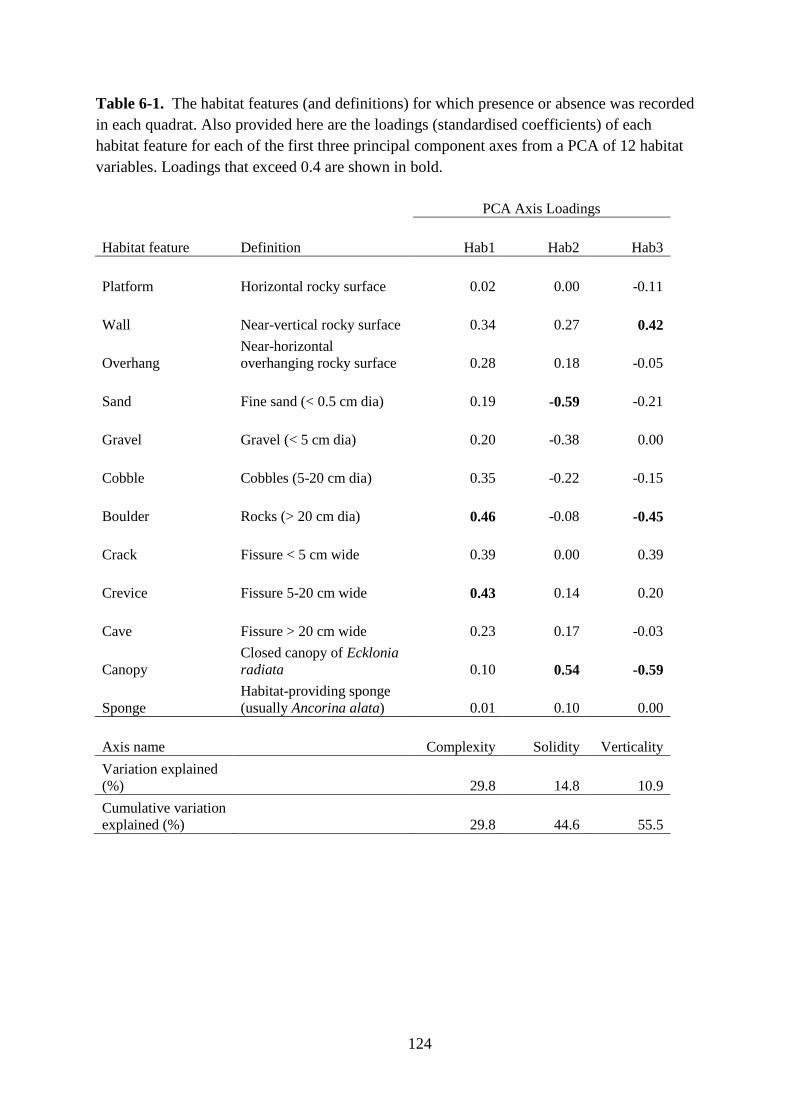
124
Table 6-1. The habitat features (and definitions) for which presence or absence was recorded
in each quadrat. Also provided here are the loadings (standardised coefficients) of each
habitat feature for each of the first three principal component axes from a PCA of 12 habitat
variables. Loadings that exceed 0.4 are shown in bold.
PCA Axis Loadings
Habitat feature Definition Hab1 Hab2 Hab3
Platform Horizontal rocky surface 0.02 0.00 -0.11
Wall Near-vertical rocky surface 0.34 0.27 0.42
Overhang
Near-horizontal
overhanging rocky surface 0.28 0.18 -0.05
Sand Fine sand (< 0.5 cm dia) 0.19 -0.59 -0.21
Gravel Gravel (< 5 cm dia) 0.20 -0.38 0.00
Cobble Cobbles (5-20 cm dia) 0.35 -0.22 -0.15
Boulder Rocks (> 20 cm dia) 0.46 -0.08 -0.45
Crack Fissure < 5 cm wide 0.39 0.00 0.39
Crevice Fissure 5-20 cm wide 0.43 0.14 0.20
Cave Fissure > 20 cm wide 0.23 0.17 -0.03
Canopy
Closed canopy of Ecklonia
radiata 0.10 0.54 -0.59
Sponge
Habitat-providing sponge
(usually Ancorina alata) 0.01 0.10 0.00
Axis name
Complexity Solidity Verticality
Variation explained
(%)
29.8 14.8 10.9
Cumulative variation
explained (%)
29.8 44.6 55.5

125
At each site, 2–4 scuba divers surveyed a total of n = 8 transects measuring 1 m wide
by 5 m long. For each transect, a measuring tape was laid on a roughly horizontal piece of
reef prior to surveying, with the ends of the tape fixed at least 2 m from the ends of the
transect to minimize disturbance to the fish. Transects were comprised of five individually-
surveyed contiguous 1 m by 1 m quadrats, with the widths delineated visually by estimating a
distance of 50 cm either side of the tape. In each quadrat, the diver first visually searched and
recorded counts for all benthic fishes, then recorded the presence or absence of a set of
predefined habitat features (Table 6-1). Cracks, crevices, and caves were searched with the
aid of a torch. One common species of triplefin, Forsterygion maryannae, was excluded from
analyses because, unlike other triplefins, it usually schools in the water column, often above
the kelp canopy. A total of 752 transects (3,760 m2) were surveyed.
Statistical modelling
For all analyses, the data were summed within transects, yielding a density for each
species of fish per five m2, and a score from zero to five for each habitat feature, according to
the number of quadrats in which the feature was observed. A principal component analysis
(PCA) of the habitat scores reduced the dimensionality of the habitat information and
identified important gradients in habitat structure. Three PCA axes (Hab1, Hab2, and Hab3;
see Table 6-1) from this analysis were used as predictor variables, along with the factors
inherent in the experimental design of the study, in the models described below.
A matrix of zero-adjusted Bray-Curtis dissimilarities (Clarke et al. 2006) was used to
quantify ecological variation in assemblage structure. Partitioning of variation in this matrix
was done using permutational multivariate analysis of variance (PERMANOVA, Anderson
2001b). The predictor variables (listed in full in Table 6-3) included categorical factors
arising from the experimental design (namely Reserve status, Location, Year, Site, and all
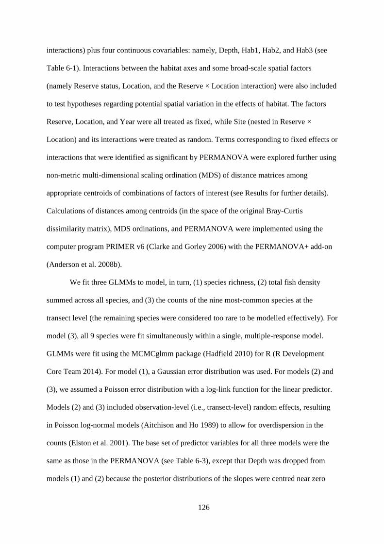
126
interactions) plus four continuous covariables: namely, Depth, Hab1, Hab2, and Hab3 (see
Table 6-1). Interactions between the habitat axes and some broad-scale spatial factors
(namely Reserve status, Location, and the Reserve × Location interaction) were also included
to test hypotheses regarding potential spatial variation in the effects of habitat. The factors
Reserve, Location, and Year were all treated as fixed, while Site (nested in Reserve ×
Location) and its interactions were treated as random. Terms corresponding to fixed effects or
interactions that were identified as significant by PERMANOVA were explored further using
non-metric multi-dimensional scaling ordination (MDS) of distance matrices among
appropriate centroids of combinations of factors of interest (see Results for further details).
Calculations of distances among centroids (in the space of the original Bray-Curtis
dissimilarity matrix), MDS ordinations, and PERMANOVA were implemented using the
computer program PRIMER v6 (Clarke and Gorley 2006) with the PERMANOVA+ add-on
(Anderson et al. 2008b).
We fit three GLMMs to model, in turn, (1) species richness, (2) total fish density
summed across all species, and (3) the counts of the nine most-common species at the
transect level (the remaining species were considered too rare to be modelled effectively). For
model (3), all 9 species were fit simultaneously within a single, multiple-response model.
GLMMs were fit using the MCMCglmm package (Hadfield 2010) for R (R Development
Core Team 2014). For model (1), a Gaussian error distribution was used. For models (2) and
(3), we assumed a Poisson error distribution with a log-link function for the linear predictor.
Models (2) and (3) included observation-level (i.e., transect-level) random effects, resulting
in Poisson log-normal models (Aitchison and Ho 1989) to allow for overdispersion in the
counts (Elston et al. 2001). The base set of predictor variables for all three models were the
same as those in the PERMANOVA (see Table 6-3), except that Depth was dropped from
models (1) and (2) because the posterior distributions of the slopes were centred near zero

127
and, while individual species have different depth ranges, there was no reason to suspect an
effect of Depth on species richness or total density. In addition to the base set of predictors
listed in Table 6-3, model (3) included a fixed factor for Species (with 9 levels), as well as: (i)
fixed interactions between Species and each of the fixed effects for Reserve, Location, Year,
and the three habitat axes; and (ii) random interactions for Species × Site, Species × Site ×
Year, and Species × Transect. For the random interactions involving Species, we fit
unstructured variance-covariance matrices (using the “us” function from the MCMCglmm
package, Hadfield 2010) to allow for non-zero correlation structure among combinations of
Species, Years, and Sites, and of Species and Transects.
Samples from the joint posterior distributions of all fitted parameters were obtained
via Markov chain Monte Carlo (MCMC). For the models of species richness and total fish
density, the MCMCs were run for a total of 13,000 iterations with a thinning rate of 1/10,
from which a burn-in of 3,000 was discarded. For the multi-species model, 1,100,000
iterations were run with a thinning rate of 1/1,000 and a burn-in of 100,000. This provided a
posterior sample of 1,000 for each of the three models. Convergence of the main parameters
of interest was tested by observing the posterior traces and checking the effective sample
sizes for parameters (Gelman et al. 2014a). For the coefficients associated with all fixed
effects, we used the default, uninformative normal prior distributions with mean zero and
variance 1e+10. Following Gelman (2006), scaled, non-central F-distributions were used as
priors for the variance components for the random effects, with the scale parameter set to 1
for species richness and to 0.3 for the total number of fish. The data and R code used to fit the
GLMMs are available in Appendix C.
We used the values of model parameters obtained from the GLMMs to calculate a set
of quantities of interest for each response variable (species richness, total fish density, and
densities of each of the nine fish species) for each iteration of the MCMC. The posterior

128
distribution of each quantity was then summarised with a point estimate (median) and a 95%
credible interval (CI, given by the 0.025 and 0.975 quantiles). If the CI for a quantity of
interest did not contain zero, this was considered as support for the hypothesis that the term
was non-zero. The quantities of interest were mean values of the response variables, or some
function of means that represented an effect size. Unless otherwise specified, means were
estimated for a Depth of 10 m and for scores of zero for each of the three Habitat axes, which
represented a standardised ‘average’ habitat. Thus, the means are adjusted (or ‘controlled’)
for any differences in Depth or Habitat among the surveys.
More specifically, the quantities of interest were: (i) the mean values of the response
variables for each of the 16 surveys, i.e., for each combination of Reserve status, Location,
and Year; (ii) the effect size for the main effect of Reserve status, calculated as the log of the
ratio of reserve vs non-reserve means; (iii) the main effects of habitat—the estimated values
of coefficients (slopes) associated with each of Hab1, Hab2, and Hab3 (see Table 6-1); and
(iv) Reserve-Habitat interactions, evaluated as the difference between estimated coefficients
for Hab1, Hab2, and Hab3 inside vs outside reserves. The nature of non-zero interactions
were further explored by estimating and plotting fitted mean densities across the full range of
values of the Habitat variable, separately for sites inside or outside reserves.
6.4 Results
Three interpretable gradients were identified in the ordination of habitat variables
which, together, accounted for 55% of the variation in habitat (Table 6-1). The first axis
(Hab1) had positive loadings for all habitat variables, particularly Cobble, Boulder, Crack
and Crevice, and can be interpreted as a measure of overall habitat ‘complexity’. Hab1
explained 30% of the variation in habitat variables, and correlated strongly with the total
number of habitat features (Pearson’s r = 0.96). The second axis (Hab2) contrasted Sand and
Gravel with closed canopy of the kelp Ecklonia radiata (Canopy) and Wall. This was

129
Figure 6-3. Boxplots showing the distribution
of values of depth and the three PCA axes for
habitat for reserve and non-reserve transects at
each location.
interpreted to represent a continuum from broken-up rock at the reef-sand boundary to the
inner reef, where there is more continuous reef substratum, enabling kelp forests to form
complete canopies. Thus, sites with low values of Hab2 are likely to be near the reef edge.
This axis will be referred to as ‘solidity’. The third axis (Hab3) primarily contrasted Boulder
and Canopy with Wall and Crack. Higher values of Hab3 likely indicate more vertical solid
reef structures as opposed to horizontal base reef with boulders (i.e. ‘verticality’). At some
locations, differences in the depth and habitat PCA scores between reserve and non-reserve
areas were apparent (Figure 6-3), highlighting the importance of taking these measures into
account when estimating the effects of reserves.
8
10
12
14
Leigh Tawharanui Hahei
De
pth
Non reserve Reserve
-2
-1
0
1
2
Leigh Tawharanui Hahei
Hab1
-3
-2
-1
0
1
2
Leigh Tawharanui Hahei
Hab2
-2
-1
0
1
2
3
Leigh Tawharanui Hahei
Location
Hab3

130
A total of 14,056 benthic reef fish were recorded from 23 taxa and 14 families (Table
6-2). Ten of these taxa were triplefin species (Tripterygiidae), including the five species most
often seen in the surveys. Around 75% of individuals belonged to the three most abundant
species, N. segmentatus, F. varium, and R. whero. The overall average observed total density
of fish was 3.74 m-2.
There was no significant main effect of Reserve status on fish assemblage structure
(PERMANOVA, Table 6-3). Locations differed significantly, and an interaction between
Reserve status and Location indicated that the reserve effect was not consistent across the
three locations. For Leigh and Tāwharanui, the shift in community structure from
assemblages inside to those outside the marine reserves occurs in a similar direction in the
multivariate space (i.e., from upper to lower parts of the MDS plot), it occurs in the opposite
direction for Hahei (Figure 6-4b). Assemblage structure was strongly associated with changes
in Habitat, as represented by the three PCA axes (Table 6-3). The effects of two of these axes,
namely Hab1 and Hab2, varied among Locations and inside vs outside reserves (see
significant interactions with Location and Reserve-by-Location, Table 6-3).
There were few consistent patterns apparent in the estimated means inside vs outside
reserves among locations and years for species richness, total fish density, or the densities of
any of the individual species (Figure 6-5). Accordingly, the GLMMs provided no strong
statistical support for consistent, overall effects of marine reserves (Figure 6-6). Mean species
richness varied between four and five species per 5-m transect, appearing slightly higher at
Tāwharanui than the other two locations (Figure 6-5a). The mean total fish density per
transect (ranging from 10 to 24) showed similar spatio-temporal patterns to species richness,
although it was considerably higher in 2012-13 at Hahei (Figure 6-5b), apparently due to
higher numbers of N. segmentatus (Figure 6-5c) and F. varium (Figure 6-5d). In the survey at
Leigh in 2011, the mean total fish density was greater inside vs outside the reserve, yielding a

131
Table 6-2. Taxa detected in the surveys, including the number of individuals of each taxon
observed in the whole dataset. Most taxa were consistently identified to species, including all
triplefins (TF). Moridae consisted mostly of the species Pseudophycis breviuscula and
Lotella rhacina. Gobiesocidae were Dellichthys morelandi or Gastrocyathus gracilis.
Acanthoclinus spp. were most likely the species A. rua, A. marilynae, or A. littoreus. The nine
most abundant species are indicated by an asterisk (*) and these were modelled individually.
Taxon Common name Family No. observed
Notoclinops segmentatus* Blue-eyed TF Tripterygiidae 4503
Forsterygion varium* Variable TF Tripterygiidae 3256
Ruanoho whero* Spectacled TF Tripterygiidae 2753
Forsterygion lapillum* Common TF Tripterygiidae 1026
Forsterygion malcolmi* Banded TF Tripterygiidae 720
Optivus elongatus* Slender roughy Trachichthyidae 550
Pempheris adspersa* Bigeye Pempheridae 520
Forsterygion flavonigrum* Yellow-black TF Tripterygiidae 366
Parablennius laticlavius* Crested blenny Blenniidae 141
Scorpaena papillosa Dwarf scorpionfish Scorpaenidae 68
Moridae Morid cod Moridae 51
Acanthoclinus spp. Rockfish Plesiopidae 25
Karelepis stewarti Scaly-headed TF Tripterygiidae 18
Gymnothorax prasinus Yellow moray Muraenidae 16
Gobiesocidae Clingfish Gobiesocidae 10
Ruanoho decemdigitatus Long-finned TF Tripterygiidae 8
Conger verreauxi Conger eel Congridae 6
Gobiopsis atrata Black goby Gobiidae 6
Thalasseleotris iota Pygmy sleeper Eleotridae 5
Ericentrus rubrus Banded weedfish Clinidae 4
Notoclinops caerulepunctus Blue-dot TF Tripterygiidae 2
Cryptichthys jojettae Cryptic TF Tripterygiidae 1
Hypoplectrodes sp. Half-banded perch Serranidae 1

132
Table 6-3. Permutational multivariate analysis of variance (PERMANOVA) tests for the
effects of variables on the structure of assemblages of benthic reef fish, based on Bray-Curtis
distances of the transect-level abundance of all species. There were 635 residual df, and tests
were based on Type III partial sums of squares and 999 permutations.
Source df Pseudo-F P-value
Hab1 1 51.83 0.001 ***
Hab2 1 10.41 0.001 ***
Hab3 1 7.29 0.001 ***
Hab1 × Res 1 1.41 0.206
Hab2 × Res 1 1.66 0.132
Hab3 × Res 1 1.30 0.235
Hab1 × Loc 2 2.47 0.002 **
Hab2 × Loc 2 1.98 0.026 *
Hab3 × Loc 2 1.47 0.113
Hab1 × Res × Loc 2 3.58 0.001 ***
Hab2 × Res × Loc 2 1.98 0.017 *
Hab3 × Res × Loc 2 0.99 0.471
Depth 1 2.67 0.009 **
Reserve 1 1.51 0.193
Location 2 4.81 0.002 **
Year 2 6.74 0.001 ***
Res × Loc 2 2.03 0.040 *
Res × Year 2 1.34 0.185
Loc × Year 3 5.38 0.001 ***
Site (Loc × Res) 29 6.55 0.001 ***
Site (Loc × Res) × Year 49 2.32 0.001 ***
Res × Loc × Year 3 1.46 0.104

133
Figure 6-4. Non-metric multidimensional scaling (MDS) plots of (a) the Site-by-Year
centroids and (b) Location-by-Reserve-by-Year centroids, in Bray-Curtis space, shown by
Location and Reserve status (R = reserve, NR = non-reserve). The 2-d stress for the MDS
analyses were 0.13 (a) and 0.07 (b).
non-zero reserve effect in 2011 at Leigh, and in 2011 overall (Figure 6-6), seemingly due to
increased densities of N. segmentatus, R. whero, and P. laticlavius. There was marginal
support for an overall reserve effect (Figure 6-6) on N. segmentatus, with densities estimated
to be 1.446 (95% CI: 0.993–2.111) times greater inside vs outside reserves, on average. This
was primarily driven by high densities within reserves at Leigh and Tāwharanui in 2011
(Figure 6-5c). There were some non-zero differences with reserve status at some locations
and in some years (Figure 6-6). Densities of R. whero were greater inside than outside the
reserve across all years at Leigh, and across all locations in 2011. In contrast, densities of F.
lapillum were greater outside the reserve at Leigh but inside the reserve at Hahei. P.
laticlavius had greater densities, on average, inside reserves at Leigh and Tāwharanui but
outside the reserve at Hahei.
The main effects of habitat on each of the response variables were strong. Species
richness, total fish, and the densities of all but one species, namely F. lapillum, increased with
increased habitat complexity (Hab1, Figure 6-7a). In most cases, the strength of the effect
Leigh R
Leigh NRTawharanui R
Tawharanui NRHahei RHahei NR
(a)2011
2011
2011
2011
2011
2011
2012
2012
2012
2012
2012
2012
2013
2013
2013
2013
(b)

134
Figure 6-5. Estimated mean densities per 5-m2 transect for each combination of Location,
Reserve status, and Year, with 95% credible intervals, for (a) species richness, (b) total
number of fish, and (c–k) each of the nine most-common species. Estimates are for a
standardised median habitat at a depth of 10 m. In some cases, the y-axes for (e–k) are shown
on a square-root scale for clarity.
Leigh Tawharanui Hahei
0
2
4
6
2011 2012 2013 2011 2012 2013 2011 2012 2013
(a) Species richness
Leigh Tawharanui Hahei
0
10
20
30
2011 2012 2013 2011 2012 2013 2011 2012 2013
(b) Total density of fishes
Leigh Tawharanui Hahei
0
5
10
2011 2012 2013 2011 2012 2013 2011 2012 2013
(c) Density of N. segmentatus
Leigh Tawharanui Hahei
0
3
6
9
2011 2012 2013 2011 2012 2013 2011 2012 2013
(d) Density of F. varium
Leigh Tawharanui Hahei
0
2
4
6
2011 2012 2013 2011 2012 2013 2011 2012 2013
(e) Density of R. whero
Leigh Tawharanui Hahei
0
2
468
2011 2012 2013 2011 2012 2013 2011 2012 2013
(f) Density of F. lapillum
Leigh Tawharanui Hahei
0
1
23
2011 2012 2013 2011 2012 2013 2011 2012 2013
(g) Density of F. malcolmi
Leigh Tawharanui Hahei
0.00
0.25
0.500.75
2011 2012 2013 2011 2012 2013 2011 2012 2013
(h) Density of O. elongatus
Leigh Tawharanui Hahei
0.0
0.1
0.20.30.4
2011 2012 2013 2011 2012 2013 2011 2012 2013
(i) Density of P. adspersa
Leigh Tawharanui Hahei
0.0
0.4
0.81.21.6
2011 2012 2013 2011 2012 2013 2011 2012 2013
(j) Density of F. flavonigrum
Leigh Tawharanui Hahei
0.0
0.5
1.01.52.0
2011 2012 2013 2011 2012 2013 2011 2012 2013
(k) Density of P. laticlavius
Reserve
Non reserve

135
Figure 6-6. Estimated main effects of marine reserves, shown here as means and 95%
credible intervals of the log ratios of Reserve vs Non-reserve means. They are shown for the
overall study (i.e. calculated from reserve and non-reserve means that were averaged, or
‘marginalised’, across all Location-Year combinations), for each Location (averaged across
Years), and for each Year (averaged across Locations). Filled circles indicate that the 95%
credible interval does not contain zero, suggesting a non-zero difference associated with
Reserve status. These estimates are standardised for habitat and depth using Bayesian
hierarchical models.
Sp. richness Total f ish N. segmentatus F. v arium R. whero
Ov erall
Hahei
Tawharanui
Leigh
2013
2012
2011
Hahei 2013
Hahei 2012
Hahei 2011
Tawharanui 2012
Tawharanui 2011
Leigh 2013
Leigh 2012
Leigh 2011
L
oca
tion
sY
ears
Lo
ca
tion
s b
y Y
ea
rs
-0.2 0.0 0.2 0.4-0.5 0.0 0.5 1.0 -0.5 0.0 0.5 1.0 1.5-0.5 0.0 0.5 -1 0 1
F. lapillum F. malcolmi O. elongatus P. adspersa F. f lav onigrum P. laticlav ius
Ov erall
Hahei
Tawharanui
Leigh
2013
2012
2011
Hahei 2013
Hahei 2012
Hahei 2011
Tawharanui 2012
Tawharanui 2011
Leigh 2013
Leigh 2012
Leigh 2011
L
oca
tion
sY
ears
Lo
ca
tion
s b
y Y
ea
rs
-4 -2 0 2 4 6 -1 0 1 -2 0 2 4 -4 0 4 -2 0 2 -15-10 -5 0 5
Posterior estimates of the reserve effect (log reserve:non-reserve ratio)

136
Figure 6-7. Coefficients associated with the habitat axes, represented by the means and 95%
CIs of the posterior distributions of coefficient values, estimated for the overall study and for
each Location. Symbols for which the CI does not contain zero are filled, suggesting
evidence for a non-zero habitat association.
Sp. richness Total fish N. segmentatus F. varium R. whero F. lapillum
F. malcolmi O. elongatus P. adspersa F. flavonigrum P. laticlavius
Hahei
Tawharanui
Leigh
Overall
Hahei
Tawharanui
Leigh
Overall
0.0 0.5 1.0 0.0 0.2 0.4 0.0 0.2 0.4 0.0 0.1 0.2 0.0 0.2 0.4 0.6 -0.5 0.0 0.5
0.0 0.2 0.4 0.6 0 1 2 0 2 0.0 0.5 -1 0 1 2
(a) Coefficients for Hab1
Sp. richness Total fish N. segmentatus F. varium R. whero F. lapillum
F. malcolmi O. elongatus P. adspersa F. flavonigrum P. laticlavius
Hahei
Tawharanui
Leigh
Overall
Hahei
Tawharanui
Leigh
Overall
0.0 0.2 0.4 0.0 0.1 0.2 0.0 0.1 0.2 0.3 -0.1 0.0 0.1 0.0 0.1 0.2 -0.6 -0.4 -0.2 0.0
0.0 0.2 0.4 0.6 0.0 0.5 1.0 0 1 2 3 -0.5 0.0 0.5 1.0-1.0 -0.5 0.0 0.5
(b) Coefficients for Hab2
Sp. richness Total fish N. segmentatus F. varium R. whero F. lapillum
F. malcolmi O. elongatus P. adspersa F. flavonigrum P. laticlavius
Hahei
Tawharanui
Leigh
Overall
Hahei
Tawharanui
Leigh
Overall
-0.2 0.0 0.2 0.0 0.1 0.2 0.0 0.2 0.0 0.1 0.0 0.1 0.2 -0.5 0.0
-0.4 -0.2 0.0 0.2 -0.5 0.0 0.5 -1 0 1 -1.0 -0.5 0.0 0.5 -1 0 1
Estimated values of coefficients
(c) Coefficients for Hab3

137
Figure 6-8. Reserve-Habitat interactions, represented by the means and 95% CIs of the
posterior distributions of the differences between the habitat coefficients inside vs outside
reserves, estimated for the overall study and for each Location. Symbols for differences for
which the CI does not contain zero are filled, representing evidence for a non-zero
interaction.
Sp. richness Total fish N. segmentatus F. varium R. whero F. lapillum
F. malcolmi O. elongatus P. adspersa F. flavonigrum P. laticlavius
Hahei
Tawharanui
Leigh
Overall
Hahei
Tawharanui
Leigh
Overall
0.0 0.5 0.0 0.2 -0.2 0.0 0.2 0.0 0.5 0.0 0.5 -1.5 -1.0 -0.5 0.0
0.0 0.5 1.0 -2 0 -2 0 2 4 0 1 -4 -2 0
(a) Differences between reserve and non-reserve coefficients for Hab1
Sp. richness Total fish N. segmentatus F. varium R. whero F. lapillum
F. malcolmi O. elongatus P. adspersa F. flavonigrum P. laticlavius
Hahei
Tawharanui
Leigh
Overall
Hahei
Tawharanui
Leigh
Overall
-0.5 0.0 0.5 0.0 0.2 -0.2 0.0 0.2 0.0 0.2 0.4 -0.2 0.0 0.2 -0.5 0.0 0.5
-1.0 -0.5 0.0 0.5 -1 0 1 2 -2 0 2 -1 0 1 -1 0 1 2
(b) Differences between reserve and non-reserve coefficients for Hab2
Sp. richness Total fish N. segmentatus F. varium R. whero F. lapillum
F. malcolmi O. elongatus P. adspersa F. flavonigrum P. laticlavius
Hahei
Tawharanui
Leigh
Overall
Hahei
Tawharanui
Leigh
Overall
-1.0 -0.5 0.0 0.5 -0.2 0.0 0.2 -0.2 0.0 0.2 -0.2 0.0 0.2 -0.4 -0.2 0.0 0.2 -1.0 -0.5 0.0 0.5
-1.0 -0.5 0.0 0.5 -1 0 1 2 -2 0 2 -1 0 1 -2 -1 0
Reserve minus non-reserve habitat coefficients
(c) Differences between reserve and non-reserve coefficients for Hab3

138
Figure 6-9. Exploration of Reserve-Habitat interactions, represented here as mean densities
across the range of values of the habitat variables, estimated separately for inside and outside
reserves, for the overall study and for each Location. Hab1 represents a gradient of increasing
complexity, and Hab2 represents a gradient of sandy broken-up reef to solid reef with closed
Ecklonia canopy. The y-axes are shown on a square-root scale for clarity.

139
varied to some extent among locations. Transects on broken, sandy habitat near the edges of
reefs (i.e. lower values of Hab2) had, on average, fewer species and total fish than those on
less sandy transects with closed Ecklonia canopy (higher values; Figure 6-7b). Likewise, five
of the nine species also showed positive relationships with Hab2, while F. varium, F.
flavonigrum, and P. laticlavius showed no overall relationship, and F. lapillum had a negative
relationship. Total fish density and densities of N. segmentatus and R. whero were positively
associated with verticality (Hab3, Figure 6-7c).
Reserve-Habitat interactions, consistent across locations, were identified for four
species: R. whero, F. lapillum, and F. flavonigrum with Hab1 (Figure 6-8a), and F. varium
with Hab2 (Figure 6-8b). No interactions with Hab3 were evident (Figure 6-8c). On average,
densities of R. whero (Figure 6-9a) and F. flavonigrum (Figure 6-9c) were estimated to be
greater in more complex, feature-rich habitats (i.e. higher Hab1 scores) both inside and
outside reserves, but the relationships with Hab1 were stronger inside reserves. In general,
higher densities occurred in more complex habitats inside reserves compared to similarly
complex habitats outside reserves. Densities of F. lapillum were negatively associated with
complexity inside reserves but positively associated with complexity outside reserves (Figure
6-9b), although there was some variation in these relationships among locations. Associations
between F. varium and Hab2 differed for Reserves vs Non-reserves (Figure 6-9d); at all three
locations, densities were higher, on average, on inner reefs than at the edges of reefs inside
reserves while, outside reserves, the opposite pattern occurred. There was no strong evidence
for an overall Reserve-Habitat interaction for either species richness or total fish.
6.5 Discussion
We found no evidence for any overall main effects of marine reserves on assemblage
structure, species richness, or densities of individual species of small benthic reef fish. There
were some differences in assemblages observed between reserve and non-reserve areas, but

140
strong interactions with location and year indicated that these patterns reflect more general
spatial and temporal variation rather than any systematic effect of marine-reserve protection.
These results contrast with those of a previous study that reported lower densities of
some species inside vs outside the reserve at Leigh (Willis and Anderson 2003). There are
several potential reasons for this discrepancy, one being that the two studies used different
survey methods. The previous study used 3 m × 3 m caged rotenone stations. Although lethal
and labour-intensive, this allowed the study of small cryptic species that are not reliably
detected using visual methods (Willis 2001). For example, the clingfish Dellichthys
morelandi (< 7 cm, Francis 2012) was found in significantly greater numbers outside vs
inside the reserve. D. morelandi is strongly associated with the urchin Evechinus chloroticus
(Dix 1969), the density of which is known to be reduced by large snapper and lobster inside
marine reserves (Babcock et al. 1999). In addition, Willis and Anderson (2003) found
significantly lower densities of three common species of triplefin (F. lapillum, F. varium, and
R. whero), the total number of cryptic fish, and the species richness of cryptic fishes in kelp-
forest habitat inside vs outside reserves. In contrast, no such effects were found in the present
study. In fact, while effect sizes of zero could not be ruled out, the majority of the posterior
densities for reserve effects tended to be positive rather than negative for most species
(Figure 6-6). We consider that the inferences provided by the previous study were limited by
a lack of spatial and temporal replication. Indeed, if we considered only the data from Leigh
in the first year of the present study, we would have reported higher species richness and
densities of small benthic fishes within the reserve (Figure 6-5, Figure 6-6). This highlights
the need for empirical evaluations of the effects of reserves to be done across multiple years
and multiple locations (Willis et al. 2003b), particularly when no data are available for time
periods prior to the establishment of marine-reserve protection.

141
The lack of a main effect of reserves on densities of most species of small benthic fish
in kelp forests is perhaps not surprising when one considers the potential mechanisms. For D.
morelandi, there is a compelling mechanism due to a very strong association with a species
known to be reduced in abundance by large snapper and lobster inside reserves. For the
majority of fishes, however, an indirect effect of reserves via predation by snapper would
seem unlikely, given that snapper are generalist predators and fish do not comprise a major
part of the diet of reef-based snapper in this region (3.3% of total volume, Russell 1983).
Thus, their net trophic effect is expected to be weak for any individual taxon, particularly
fishes, which are more mobile than invertebrate prey. Blue cod (Parapercis colias,
Pinguipedidae) is another fishery-targeted predatory fish known to benefit from marine
reserves in New Zealand (Cole and Keuskamp 1998, Pande et al. 2008). It consumes fish to a
greater extent than snapper (40%, Russell 1983), but this species is relatively rare in northern
New Zealand (Smith et al. 2013) so is unlikely to exert significant trophic pressure in the
reserves examined here. Marine reserves further south where blue cod are abundant may
reduce the densities of small fishes via predation, but this requires further study.
A likely mechanism by which the three marine reserves studied here could potentially
indirectly affect assemblages of small benthic fishes is though restoration of kelp-forest
habitat via the predator-urchin-kelp trophic cascade (Babcock et al. 1999). If kelp forest
supports different assemblages than urchin-grazed habitat, then marine reserves would indeed
have broad-scale indirect effects on small fishes, as has been shown for some invertebrate
taxa (Shears and Babcock 2003). Broad-scale effects across multiple types of habitat,
including the effects of marine-reserve protection on variation in the areal extent of different
types of habitat across multiple reserves, remain to be investigated; the present study focused
instead purely on finer-scale habitat associations within kelp forests.

142
Our prediction of stronger positive associations between density and habitat
complexity (represented by PCA axis Hab1) inside vs outside reserves was realised for R.
whero and F. flavonigrum (Figure 6-9a,c). We consider that this result, combined with no
evidence for an overall difference in density in reserves, is consistent with a risk effect
whereby the fish are more strongly attracted to habitats that provide greater refuge in areas
where they detect large numbers of predators (Figure 6-1b). Reserve-habitat interactions were
also observed for F. lapillum and F. varium (Figure 6-9d), but were qualitatively different to
the prediction made in Figure 6-1b. Densities of F. lapillum were positively associated with
habitat complexity outside reserves, but negatively inside reserves (Figure 6-9b). This could
be due, in part, to R. whero or F. flavonigrum competitively excluding F. lapillum in more
complex habitat inside reserves; F. lapillum is a shallow-water species and, at 10 m, is
beyond its usual depth range (Francis 2012). Finally, F. varium appeared to be more
abundant on sandy broken reef at the sand-reef interface (i.e. low values of Hab2) outside
reserves, and on solid reef with closed Ecklonia canopy (i.e. high values of Hab2) inside
reserves (Figure 6-9d). Studies of snapper indicate that they occur in high abundance at the
sand-reef boundary (Ross et al. 2007), suggesting a risk effect for the patterns we observed
for F. varium. Manipulative experiments would be required, however, to test specific causal
mechanisms. Nonetheless, given the suspected ubiquity of risk effects in marine systems (Dill
et al. 2003) and the lack of any observed main effect of reserves on overall density, we
consider that risk effects provide compelling explanations for the different habitat
associations inside vs outside reserves observed here.
After decades of research, the full range of indirect effects of fishing, and protection
from fishing, is still poorly understood. We consider that observational studies coupled with
careful consideration of ecological mechanisms can improve our knowledge of the indirect
effects of reserves on fishes. Many past studies have employed sampling methods designed to

143
enumerate large, fishery-targeted species (e.g. 25-50 m visual transects or video-based
surveys). Data on non-targeted species are generally collected as a secondary objective, and
analysed with little consideration of the mechanisms by which indirect effects might occur or
the particular species that are likely to be affected. Broader-scale sampling methods routinely
omit small benthic species, which are often the target of predators and are thus most likely to
be indirectly affected. Moreover, there has been a narrow focus on consumptive effects (or
“density-mediated interactions”, Dill et al. 2003), focusing only on the hypothesis that
densities of prey fish are reduced by predators. Such effects can be mitigated or precluded by
behavioural plasticity, such as prey-switching by generalist predators (Roberts 1995, Jennings
and Kaiser 1998) or predator-avoidance risk effects in prey, as suggested here. To progress
our knowledge of the indirect effects of marine reserves, we must move beyond simple
evaluations of the densities of arbitrary species. We encourage a more mechanistic focus,
beginning with specifically-designed observational studies that test predictions drawn from
suspected relationships with species known to benefit from reserves and, where possible,
followed by experimental manipulations to isolate the suspected mechanisms.
6.6 Acknowledgements
This research was supported by Massey University and the Department of Conservation
(DOC, Inv 4238). I thank DOC and Clinton Duffy for logistical support and use of the
research vessel, RV Tuatini. Thanks to my supervisor Marti Anderson, who will co-author
the article when published. I also thank the following divers who helped in the field (in order
of the amount of data contributed): Oliver Hannaford, Marti Anderson, Steve Hathaway,
Severine Dewas, Paul Caiger, Clinton Duffy, Charles Bedford, Kirstie Knowles, Nick
Macrae, Sietse Bouma, Dave Culliford, Caroline Williams, and Alice Morrison.

144
Chapter 7. Could ecologists be more random?
7.1 Abstract
When conducting field studies, it is common for ecologists to choose the locations of
sampling units arbitrarily during the sampling event, rather than using a properly randomized
sampling design. Unfortunately, this so-called haphazard sampling approach cannot provide
formal statistical inference from the sample to the population without additional, largely
untestable, assumptions. Here, we argue that two recent technological advances remove the
need for haphazard sampling in many situations. A general approach to simple randomized
sampling designs is outlined, and some examples demonstrate that even complicated designs
can be implemented easily using software widely used among ecologists. We consider that
more rigorous, randomized sampling designs would strengthen the validity of the conclusions
drawn from ecological studies, to the benefit of the discipline as a whole.
7.2 Main text
Ecological studies often involve the collection of data from the field. It is rarely
practical to comprehensively survey the entire spatial domain of interest to the study (i.e. the
population). Instead, data are obtained from a sample of standardized units, such as counts of
individuals in a quadrat. Statistical inference is the process of drawing conclusions about the
population of interest from data obtained from a sample, a process which underpins much of
our knowledge of the natural world. The locations of sampling units are chosen by way of a
sampling design. Regrettably, inadequate specification of the sampling design and a
pervasive methodological shortcut, known as “haphazard”, “convenience” or “opportunity”
sampling, continue to undermine the validity of statistical inference in ecology (Anderson
2001a, Lewis 2004). Here, we argue that some of the main reasons for haphazard sampling

145
are no longer valid in many situations, as some recent technological advances make it much
easier to implement spatially-randomised sampling designs.
Two important conditions must be met to draw valid, design-based, statistical
inference from field samples (Fisher 1935): the population to which inference is intended to
apply must be explicitly defined, and sampling units must be selected from this population
using some randomisation procedure where the probability of selection for each unit is
known and is non-zero. Note that the set of potential sampling units, i.e. the sampling frame,
may differ from the population of interest if some parts of the population are unavailable for
sampling. In this case, inference from the sample strictly applies to the sampling frame, but
may be extended to the population with the assumption that the sampling frame is
representative of the population.
A sample for which the above conditions are met is called a “probability sample”,
which is achievable by a variety of sampling designs (see, e.g., Cochran 1977). The simplest
is simple random sampling, where each unit in the sampling frame has an equal probability of
being selected. Other commonly-used probability sampling designs can be easier to
implement in the field, such as systematic sampling where units are selected in a regular grid
or at fixed intervals, or two-stage methods such as stratified random or cluster sampling,
which involve dividing the sampling frame into smaller strata from which random samples
are taken. Recently, more sophisticated methods have been developed to achieve better
spatial coverage and sampling efficiency (e.g. Stevens and Olsen 2004, Grafström et al.
2012). Whatever the details of the specific sampling design, the intended population of
interest, the sampling frame and sampling design should be known and explicitly stated.
Crucially, if an appropriate randomization method is not used, units might (unwittingly) be
chosen in a way that introduces subjective selection bias (Smith 1983). Parameter estimates

146
may be then biased with respect to the population of interest, potentially leading to false
conclusions.
The importance of randomization to statistical inference dates at least as far back as
Fisher (1935), and is highlighted in the first chapters of most undergraduate statistical texts.
In spite of this, the methods used to choose sampling units are often not explicitly stated in
ecological field studies, and proper spatial randomization methods are routinely overlooked
(Table 7-1). Haphazard sampling, where units are placed opportunistically in suitable habitat
identified at the time of sampling (Andrew and Mapstone 1987), is still commonplace. This
approach cannot be considered probability sampling, as there is no formal randomization and
the probability of including any potential sampling unit is unknown. Thus, haphazard
sampling provides descriptive data for the sample at hand, but the lack of randomization and
a well-defined population and sampling frame precludes any direct, formal inference to the
population (Andrew and Mapstone 1987, Underwood 1997, Olsen et al. 1999, Anderson
2001a). Such inference requires the untestable assumption that the haphazard sampling has
not introduced any directional bias in measured quantities of interest by reference to the
underlying parameters and hypotheses being investigated (McDonald 2003).
The use of haphazard sampling is not necessarily through neglect, however. We see
two potential reasons for ecologists to use a haphazard approach instead of a properly
randomized design. Firstly, it may be genuinely difficult to sample randomly if the location
of suitable habitat is unknown prior to sampling. This can be particularly true of studies in
remote, poorly studied, or underwater environments. Inadequate knowledge of the spatial
extent of the target habitat can lead to the sampling frame being defined poorly, if at all, thus
preventing the selection of sampling units prior to the sampling event. Secondly, the
logistical matter of choosing random points within the sampling frame is another potential

147
Table 7-1. Systematic review of methods used to choose spatial sampling units in recent
ecological studies. We conducted a census of articles which resulted from a search on 7 July
2013 in Biological Abstracts. Search parameters were Year=2013, Topic=((abundan* OR
densit*)), Major Concepts=(ECOLOGY), and Source Titles=(Diversity and Distributions,
Ecological Applications, Ecology, Ecology Letters, Journal of Applied Ecology, Journal of
Animal Ecology, Journal of Ecology, Oecologia, or Oikos). We only included studies that
involved observations or experiments in the field, using spatially-replicated sampling units.
Field experiments from a single block which was then divided into subplots were excluded.
The allocation of treatments to units in experimental studies was not considered—we were
only interested in the method used to choose the spatial locations of units. A total of 99 out of
215 articles met our criteria for review.
Classification Description Percentage
of articles
Haphazard Explicitly stated that a haphazard method of choosing
sampling sites was used, or described a method that was
clearly haphazard.
12%
Not specified Did not specify how sampling units were chosen, e.g. “We
surveyed N sites in the forest”. We consider it likely that
many of these, in fact, used a haphazard method, on the basis
that the method used to choose the sites would be explicitly
stated if the trouble had been taken to use a robust method to
randomize the sampling.
43%
Targeted
specific
conditions
Selected (usually all) locations that fit particular
requirements, e.g. “We chose ponds that were most likely to
remain filled for the duration of the experiment”.
7%
Systematic Units were placed systematically on a regular grid or at fixed
intervals along a transect.
9%
Random Explicitly stated that sampling units were placed randomly.
Very few studies, if any, expounded on the exact method of
randomization, however.
12%
Mixture of
methods
Defied classification into the above categories because they
involved a mixture of methods, e.g. the sampling was
randomized at some spatial scales but not others, or units
were placed regularly along haphazardly-chosen transects.
16%

148
barrier to randomized sampling in field studies. If the sampling frame is a simple rectangle,
points may be selected by simply generating random numbers from within the bounding
geographic coordinates, which can be done with a scientific calculator or basic software
tools. However, for more complex polygons, this process very quickly becomes tedious when
randomly allocated points fall outside the domain, thus needing to be replaced. Then, it is
more efficient to use a Geographic Information System (GIS) to select random points directly
from the sampling frame, represented by points, lines or polygons. There are many specialist
GIS software packages available for implementing this. However, many of these packages
are very costly (though there are some freeware options) and they are generally not
particularly user-friendly for non-specialists. Mastering such software can take considerable
time and perhaps costly training—an inappropriate investment when used only occasionally.
As a result, the use of a properly-randomized sampling design might be neglected in favour
of haphazardly choosing units by hand on a map or at the time of sampling, simply due to the
difficulties involved with accessing and learning to use appropriate software.
We consider that these two logistical barriers to using proper randomized designs in
field studies now pose much less of a problem than they have historically. Spatially-
referenced data for many habitats and environmental variables are increasingly available, due
to the widespread use of technologies such as remote sensing, side-scan sonar, and aerial and
satellite photography. Moreover, spatial data are often made freely available online through
the websites of government agencies and research institutes (e.g. www.usgs.gov,
www.fws.gov, www.noaa.gov). Alternatively, if the required habitat is visible from satellite,
it can be manually demarcated using computer software such as Google Earth. Thus, the
identification of the location and extent of particular habitats or environmental conditions
ahead of the sampling event is now feasible to achieve at most relevant spatial scales.
Furthermore, it is now much easier to manipulate spatial data without the use of specialized

149
Box 1. General approach to random sampling with spatial data
1. Carefully define the spatial population of interest and the sampling frame. These may
comprise an administrative area, a particular habitat, a specific range of values of
environmental variables, or a combination of these.
2. Decide on the sampling approach, including the specific sampling design (e.g. simple
random, systematic, stratified random, etc.) and the sample size.
3. Obtain the spatial data necessary for demarcating the sampling frame and import them
into R (see Appendix D). In simple cases, such as when the sampling frame comprises a
single patch of forest or a marine reserve, a single polygon may be all that is required (e.g.
Figure 5–1), which might be available from a government agency. Alternatively, if the target
habitat is visible in satellite photographs, polygons, lines or points may be drawn in Google
Earth, exported as a *.kml file, and then read into R. More complex sampling frames may
require multiple spatial datasets from a variety of sources, such as specific combinations of
environmental conditions or the intersection of geographic and habitat features (e.g. Figure
5–2).
4. Integrate the spatial data into a single spatial object, if required. This object will
represent the sampling frame from which a sample will be drawn. It may be in the form of a
grid or one or more lines, polygons, or points. In simple cases, combining spatial objects can
be done in R using the function over. However, it can be more difficult when the sampling
frame requires taking the intersection of multiple polygons or lines. In this case, a useful
strategy is to first convert one object into a set of regular points or a grid (e.g. by using the
function sample with type="regular") at a scale that is fine enough to accurately
represent the sampling frame. A candidate set of points may then be produced by selecting
(using over) those which lie within the other objects that define the sampling frame (e.g.
Figure 5–2).
5. Take a random sample in accordance with the chosen design. Once the sampling frame
is represented in R, choosing sampling units using methods such as simple random,
systematic, or stratified random sampling, can generally be implemented with only a single
line of code (Figures. 5–1 and 5–2 and Appendix D).

150
GIS software. The GIS functionality available in R (R Development Core Team 2014), an
open-source statistical programming language and platform used widely by ecologists, has
greatly improved in recent years. This is largely due to the work of Roger Bivand and
colleagues in developing the sp and rgdal libraries, which contain many of the functions
provided by specialized GIS software (Bivand 2006, Bivand et al. 2008). These libraries
include functions for importing and manipulating spatial data, such as lines and polygons,
and taking samples from spatial objects using random, stratified, and systematic designs (see
Figure 7-1). Moreover, specialized libraries, such as spsurvey (Kincaid and Olsen 2013) and
spcosa (Walvoort et al. 2010), are now available in R for implementing more advanced
spatial sampling designs. Thus, ecologists who already use R need not learn new software in
order to implement randomized sampling designs or, more generally, analyse and map spatial
data.
In light of these technological developments, we encourage ecologists who still use
haphazard sampling, and editors and referees of their articles, to carefully consider whether
this approach is still justified in their study systems. While such a plea has been made
previously (Anderson 2001a, Lewis 2004), we consider that there is now even greater
impetus for ecologists to improve their study designs. To assist the uptake of randomized
sampling, we provide a general approach for using spatial data in the planning of field studies
in Box 1, with examples in Figures 5–1 and 5–2, and code in Appendix D.
In summary, we consider that two recent developments—the greater availability of
GIS data and improved spatial functionality of free software already familiar to ecologists—
largely remove the need for haphazard sampling in many situations. We acknowledge,
however, that the haphazard approach may still be justifiable at some spatial scales,
particularly for sampling within fine-scale habitats that are beyond the resolution of currently

151
Figure 7-1. Three simple sampling designs for selecting 20 sites (pluses) from within
Tāwharanui Marine Reserve (orange) off Tāwharanui Peninsula (grey), near Auckland, New
Zealand. All three designs were implemented in R by applying the function spsample to a
polygon object Strata, in which the reserve is represented by four strata equally spaced
along the seaward border. The designs shown are (1) Simple Random Sample—points
selected randomly through the entire reserve [spsample(Strata, n=20,
type="random")]; (2) Systematic Sample—points selected on a regular grid
[spsample(Strata, n=20, type="regular")]; (3) Stratified Random Sample—five
points selected from each of the four strata [lapply(Strata@polygons, spsample,
n=5, type="random")]. Note that, in the latter case, five sites were taken from within
each of the four strata for simplicity. In practice, it may be more efficient to allocate samples
proportional to the stratum areas, which are straightforward to calculate in R (Table 2). These
designs were all implemented using only freely available data. See Appendix D for further
details, including full R code and data.

152
Figure 7-2. A more complex sampling design for Tāwharanui Marine Reserve (see Figure
7-1) targeting specific habitat and depth in four strata. The sampling frame and population of
interest here was rocky reef habitat at depths of five meters. Panel A shows three spatial
objects, representing the marine reserve (Strata, orange polygon), rocky reef (Reef, blue
polygon) and a 5-m contour (Contour, black line). Three steps were taken to obtain the
sample, as follows: 1. Convert the contour into regular points [Pts <-
spsample(Contour, n=1000, type="regular")]. Note that, for clarity, only 100
points are shown in Panel B. 2. The points that overlie reef (black dots, panel B) are selected
as candidate points while those that do not (white dots) are discarded [PtsR <-
Pts[!is.na(over(Pts, Reef)),]]. 3. Randomly select five points from the candidates
in each stratum (pluses in panel C) [PtsRS <- tapply(PtsR, over(PtsR,
Strata)$Name, sample, size=5)]. See Appendix D for further details, including full R
code and data.

153
available GIS data. Indeed, spatial information is only as useful as its resolution and accuracy
will allow. Nonetheless, our aim here is to highlight some fundamental statistical principles
of experimental design that seem largely forgotten to many ecologists. First, we encourage
that the spatial population to which inferences are to be made (and the sampling frame if
different from the population) be explicitly defined and mapped. Second, the locations of
sampling units should be chosen from this population by some randomized, repeatable
process. Third, our literature review (Table 7-1) highlights a need for more explicit
descriptions in the ecological literature of the methods used to place sampling units in the
field. Increased uptake of this general approach may eliminate unknown biases from many
future field studies, thus improving the statistical rigor of ecological science and the validity
and verifiability of its conclusions. After all, this is now much easier than ever before.
Acknowledgements
This work was supported by Massey University and the Department of Conservation (DOC
Inv 4238). I thank my supervisors Marti Anderson and Matthew Pawley who will be co-
authors on this article when published. I also thank Daniel Breen and Clinton Duffy of DOC
for providing the rocky reef polygon (Figures. 5–1 and 5–2 and Appendix D).

154
Chapter 8. General discussion
The central purpose of this thesis was to develop hierarchical Bayesian generalised
linear mixed models for complex and problematic datasets of counts of organisms, with a
specific application to evaluating potential direct and indirect effects of marine reserves on
fishes. As such, this work spans two important scientific fields, contributing new data and
fundamental scientific knowledge to the field of marine ecology alongside new methodology
and synthesis within the field of statistical modelling. In this final chapter, I aim to, firstly,
outline the contributions of this thesis to our knowledge of the ecological effects of marine
reserves and, secondly, provide a discussion and synthesis of the analytical approaches used
in this thesis and the contributions made to statistical methodology. Potential areas of future
research are discussed throughout.
8.1 Ecological effects of marine reserves
Chapters 5 and 6 contribute to our understanding of direct and indirect effects of
marine reserves by modelling counts of fishes inside vs outside three marine reserves in
north-eastern New Zealand; namely, Cape-Rodney-Okakari-Point (Leigh), Tāwharanui, and
Te Whanganui-A-Hei (Hahei) Marine Reserves. Chapter 5 presents complex hierarchical
Bayesian models of the effects of the reserves on the relative density of snapper (Pagrus
auratus: Sparidae), a species that is important both economically, in that it supports major
commercial and recreational fisheries in this region (Maunder and Starr 2001), and
ecologically, in its role in a predator-urchin-kelp trophic cascade on rocky reefs (Babcock et
al. 1999, Shears and Babcock 2003, Shears et al. 2008). Accurate quantification of the effects
of marine reserves on such a species is essential for understanding and predicting the
potential benefits of marine reserves to fished populations within and beyond the boundaries

155
of the reserves, and the potential extent of any indirect effects. As such, these results are of
fundamental importance to resource managers.
Counts of snapper above the then-legal size limit of 27 cm fork-length (i.e., “legal-
sized” snapper) were estimated, on average, to be 13-times greater inside vs outside reserves
(Table 5-4). In contrast, there was no evidence of an effect of protection on fish below the
legal size. An interaction between reserve status and location indicated that the effect size for
legal-sized snapper varied among the three reserves. The estimated effect size ranged from
19-fold greater relative densities inside the reserve near Leigh, to 8-fold greater at
Tāwharanui. Potential reasons for the interaction were discussed, and likely include a range
of factors such as differences in reserve size, habitat, the extent of illegal fishing inside the
reserve, and patterns of inshore migration of adult fish.
As demonstrated here for snapper, many marine reserves worldwide have successfully
restored high densities of large, fishery-targeted, predatory species (Molloy et al. 2009,
Claudet et al. 2010, Guidetti et al. 2014), potentially reintroducing functional processes back
into the ecosystem that had, in some cases, been effectively eliminated by fishing
(Friedlander and DeMartini 2002, Eddy et al. 2014). Where these processes are strong,
marine reserves can have indirect effects, potentially modifying the behaviour or abundance
of other organisms, including those not targeted by fishing (Pinnegar et al. 2000). The
flagship example of this in temperate rocky reefs is the predator-urchin-kelp trophic cascade
(Ling et al. 2015). Where this occurs, the densities of the species involved are largely
controlled by trophic processes: predation by snapper and lobster can limit urchin densities,
and herbivory by urchins can limit kelp in the absence of predators. Top-down trophic control
of abundance, and especially trophic cascades which involve more than two trophic levels, is
very context-dependent, requiring strong and spatially and temporally consistent trophic links
among the levels (Polis 1994). Trophic effects can be superseded by a range of potential

156
mitigating factors (Polis and Strong 1996). In the predator-urchin-kelp example, abiotic
factors such as wave action and sedimentation (Shears et al. 2008) and biotic factors such as
disease (Shears and Ross 2010) can limit numbers of urchins and/or kelp, potentially
decoupling the trophic links that generate the indirect cascade effect of predators on kelp.
While trophic cascades have been recorded in many ecosystems, including aquatic ones
(Pinnegar et al. 2000), they are thought to be relatively rare phenomena across the full range
of biological food webs (Strong 1992).
Much of the research into indirect ecological effects of marine reserves has focused
on the process of predation. In recent years, there is a growing awareness of the potential of
the presence of particular species to invoke changes in the behaviour of others, referred to as
“behaviourally-mediated indirect interactions” or, more generally, “risk effects” (Dill et al.
2003, Heithaus et al. 2008). Indeed, in the context of the predator-urchin-kelp trophic cascade
on New Zealand rocky reefs, juvenile urchins inside reserves more often exhibited cryptic
behaviour, where they hide in cracks in the rock, feeding primarily on drifting fragments of
dead algae (Shears and Babcock 2003). This change in behaviour, assumed to be a response
to abundant would-be predators, may help to reduce the consumption of live kelp plants by
urchins, thereby strengthening the cascade effect.
The focus of Chapter 6 was to evaluate evidence for indirect effects of protection by
marine reserves on assemblages of small benthic reef fishes. I (along with an army of divers)
collected a large hierarchically structured dataset of counts of several species of small benthic
reef fish, along with the presence of relevant habitat features, inside and outside the same
three marine reserves in north-eastern New Zealand (the same as those studied in Chapter 5)
over three summers. In contrast with a previous study (Willis and Anderson 2003), there was
no evidence for overall main effects of reserves on species richness or the densities of any
species (Figure 6-6). Densities and richness were strongly associated with gradients in habitat

157
features, particularly the overall feature-richness or ‘habitat complexity’ (Figure 6-8).
Furthermore, for some species, there was evidence for differences in habitat associations
inside vs outside marine reserves (Figure 6-8). In particular, inside reserves, two common
species (namely, Ruanoho whero and Forsterygion flavonigrum) were more strongly
associated with habitat complexity than outside reserves (Figure 6-9). These results suggest
that predation of small benthic reef fish has not substantially increased inside reserves.
Instead, results are consistent with a risk effect, where the small fish detect high abundances
of larger predators inside reserves and are thus more strongly attracted to habitat features that
provide potential shelter from predators.
The assemblages of small benthic fishes under study here, generally dominated by
endemic species of triplefin (Tripterygiidae), are an important and unique part of the
biodiversity of New Zealand coasts. From a conservation-management perspective, the
finding that overall densities are likely unaffected by marine reserves, at least in north-eastern
New Zealand, is somewhat comforting; it suggests that reserves might be established here
with no great concern for negative impacts on the diversity and abundance of these
assemblages. The results are also compelling from an ecological perspective. Fish are often
found in the gut of snapper, but they make up a small proportion of their diet (e.g., an
estimated 3.3% of total volume, Russell 1983). Snapper are highly generalist predators, and
as such can readily switch among prey species according to their relative availability.
Invertebrates may be more accessible prey for snapper than fishes, particularly in complex
habitats, due to the latter being highly mobile. Generalist predators are expected to have
diffuse effects on the abundance of any particular prey species and community structure in
general (Polis and Strong 1996). For many marine species, bottom-up processes such as
recruitment and intra-specific competition are generally considered to be more important for
determining relative abundances than top-down processes such as predation (Polis 1994,

158
Polis and Strong 1996, Jennings and Kaiser 1998). Comparatively, there is a growing view
that risk effects—effects of predators on the behaviour of prey—may be more prevalent than
previously thought (Lima and Dill 1990, Dill et al. 2003, Heithaus et al. 2008). Yet, risk
effects are relatively poorly understood, perhaps because they are less conspicuous and more
difficult to quantify than effects on abundance. Risk-averse behaviour of prey species may
have as yet unseen ecological effects on community dynamics. For example, the reserve-
habitat interaction observed here for some triplefin species indicates that highly complex
habitats inside reserves would have greater densities of fishes than highly complex habitats
outside reserves. Also, less complex habitats inside reserves would have lower densities of
fishes than less complex habitats outside reserves. Thus, there is greater variance in
assemblages across the complexity gradient inside reserves, which may increase the spatial
variation in ecological processes such as intra- and inter-specific competition for resources
and predation. Spaces left available in low complexity habitat may be filled by other species
less threatened by predation. Spatial variation in ecological processes may result in spatial
variation in community structure (i.e., beta-diversity, Anderson et al. 2011), mediated by
patterns in fine-scale habitat structure.
These results suggest several areas of potentially fruitful ecological research. The
various stimuli that might alert triplefins to the presence of predators and induce stronger
habitat associations, such as olfactory and visual cues, could be experimentally manipulated
in aquaria to identify the potential mechanisms responsible for the risk effects. Further
observational studies may reveal that changes in the behaviour of triplefins might have
secondary effects on fine-scale patterns in the structure and diversity of local communities
with which they interact, including prey and/or competitors. More broadly, many studies
have sought evidence for indirect effects of marine reserves on the abundance of non-targeted
fishes via predation, yet only a few examples have been found to support this idea (e.g.

159
McClanahan et al. 1999, Graham et al. 2003, Watson et al. 2007, Edgar and Stuart-Smith
2009) and meta-analyses suggest no overall mean effect of marine protection on abundances
of non-targeted reef fishes (Mosquera et al. 2000, Micheli et al. 2004, Claudet et al. 2010).
The focus of this prior research has largely been limited to evaluating effects on prey
abundance, typically disregarding any potential effects of restored populations of predators
on the behaviour of their prey. Further examination of the relationships between prey species
and habitat with and without predators in this and in other systems may indicate potential
mechanisms by which prey avoid predation.
8.2 Statistical methodology
Chapters 1 and 2 discussed some statistical challenges that are often encountered
when modelling ecological count data, including complex, unbalanced experimental designs,
multiple hierarchical mixed effects, and overdispersed and zero-inflated errors. Recent
advances in statistical methodology, which are reviewed in Chapter 2, has meant that
modellers are now better equipped to cope with these challenges, particularly with the rise of
Bayesian MCMC and generalised linear mixed models (GLMMs), with non-standard error
distributions that can account for general overdispersion and excess zeros. Where, in the past,
ecologists have had to shoehorn their data into traditional models (by, for example, ignoring
the inconvenient aspects of the experimental design, excluding troublesome data, and
transforming response variables), they are now better able to adapt their models to their data
(Bolker et al. 2009, Ellison and Dennis 2009). Yet, there is still room for improvement. One
of the next important areas of research is to improve methods for modelling data that poses
multiple challenging features. For example, for unbalanced designs, fitting GLMMs with
multiple random effects using a conventional likelihood-based approach is often
computationally infeasible (Bolker et al. 2009). To meet these challenges, ecologists are
increasingly turning to Bayesian Markov Chain Monte Carlo (MCMC) methods. These

160
methods provide a highly flexible framework for statistical modelling, and one can fit highly
complex models and simultaneously quantify uncertainty across the full set of model
parameters, including multiple random effects. This thesis developed and applied Bayesian
GLMM methodology for ecological count data, inspired while analysing two challenging
datasets: one of counts of snapper, and one of counts of several small benthic fish species.
While both analyses centred on a Bayesian GLMM approach, they necessarily differed in
many respects, including the nature of the research questions, the structure of the data
(univariate vs multivariate responses and error structure), presentation of the results, and the
software used. In this section, I will compare the two analyses and outline the major
contributions of this thesis to statistical methodology.
For the snapper project, there was little a priori doubt of the existence of a reserve
effect for legal-sized snapper; this had been shown by several previous studies (using simpler
modelling tools) in this region (Millar and Willis 1999, Willis et al. 2003a, Denny et al. 2004)
and is, frankly, quite evident to anyone who has donned a mask and snorkel inside and
outside reserves. Thus, the focus of this study was not to evaluate evidence for a reserve
effect per se, but rather to accurately quantify the reserve effect, along with spatio-temporal
variation in this effect. In order for this to be as rigorous as possible, the model needed to
account for the overdispersion caused by high variability and the high proportion of zero
occurrences in the count dataset. Some of this overdispersion could naturally be accounted
for by fitting models that included the various sources of spatial and temporal variation in the
experimental design. Yet, even within these models, the counts exhibited greater variance and
incidence of zeros than the usual commonly used error distributions would allow. Failure to
model such overdispersion can lead to inaccurate estimates of uncertainty for the parameters
of interest.

161
Exploratory modelling of the zero-inflation and overdispersion in counts of snapper
led me to an idea originally proposed by Lambert (1992) in her seminal paper in
Technometrics on zero-inflated methods for modelling counts of faults in manufacturing
processes. The idea was that, in a zero-inflated model (such as the one described in Equation
(4-1)), the mean of the count distribution, 𝜆, and the probability of an excess zero, 𝜋, could be
functionally related; in this case, such a relationship could be modelled explicitly with the
structure logit(𝜋) = −𝜏 log (𝜆). I fitted a modified version of this structure, logit(𝜋) = 𝛾0 +
𝛾1log (𝜆), with a negative binomial error structure for the counts within a Bayesian model for
legal-sized snapper. This method, termed “linked zero inflation” and presented in Chapter 4
and Smith et al. (2012), provided several advantages over the more conventional alternatives:
it provided a better fit to the data with fewer parameters, was computationally well-behaved,
and allowed for relatively straightforward interpretation of model parameters. Moreover,
functionally linking 𝜆 and 𝜋 is consistent with an ecological phenomenon known as the
occupancy-abundance relationship (Borregaard and Rahbek 2010). Chapter 3 of this thesis
provided a review of the various processes that give rise to zero counts in ecology, and
developed some potentially useful approaches to analysing relationships between occupancy
and abundance, particularly in light of the debate of whether it is an ecological phenomenon,
or merely a statistical one (Wright 1991, Hartley 1998, Nielsen et al. 2005, Sileshi et al.
2009). Strictly speaking, a model with a linked zero-inflated error structure is not technically
a generalised linear model, as the resulting distribution is unlikely to be a member of the
exponential family of distributions (see McCullagh and Nelder 1989). Nonetheless, the linked
zero inflation error structure provides a parsimonious option where the occurrence of excess
zeros is indeed related to the mean count, and is perhaps the most important contribution of
this thesis to statistical methodology. The broader applicability of the method to counts of
other organisms has yet to be fully explored, although the method was applied recently to

162
counts of fishes in a broad-scale evaluation of the effects of the Great Barrier Reef Marine
Park, published in Current Biology (Emslie et al. 2015).
Ecological studies often involve hierarchical sampling designs with replication across
a variety of spatial and temporal scales (García-Charton and Ruzafa 1999). Explicitly
modelling the variation attributable to each random effect arising from such designs is
important, as it can improve levels of uncertainty and provide a useful comparison against
estimates of detectable reserve effects (García-Charton et al. 2000, 2004). Analysis of
variance (ANOVA; Fisher 1935, Scheffé 1959) provides a useful general framework for
analysing data from hierarchical sampling designs, representing each level of replication as a
batch of effects (Gelman 2005). Historically, ANOVA tables have focused on presenting the
mean squares, F-statistic, and p-values to test the statistical significance for each term. Many
authors, including non-Bayesians, have criticised the null-hypothesis testing approach
(Reckhow 1990, Johnson 1999, Anderson et al. 2000), and many have recently argued in
favour of presenting the results of ANOVA models in terms of variance components
(Graham and Edwards 2001, Gelman 2005, Qian and Shen 2007, Qian et al. 2009, 2010,
Hector et al. 2011). Variance components (i.e., the variance among the levels of a factor)
provide a more useful basis for directly comparing the magnitude of the effects of each term
than the classical mean square, F-ratio, or p-value. Variance components can be simpler to
calculate than F-ratios, which require the specification of correct expected mean squares for
each term—a complicated task for mixed models, particularly for unbalanced designs
(Graham and Edwards 2001, Searle et al. 2009). Moreover, with MCMC methods, it is
straightforward to obtain joint posterior distributions for variance components for complex
multi-factor models, and summarise these with point estimates and uncertainty intervals.
Chapter 2 reviewed this methodology, extending the ANOVA framework outlined by
Gelman (2005) to GLMMs. These methods were then implemented in Chapters 4 and 5 to

163
estimate variance components associated with each source of variation inherent in the design
of the snapper monitoring programme. In the application presented here, variance
components identified the reserve effect as by far the greatest source of variation in counts of
legal-sized snapper, and provided a basis for comparing the spatial and temporal sources of
variation, including the reserve effect (Figure 5-2).
The second major project in this thesis was a study of indirect effects of reserves on
assemblages of small benthic fishes (Chapter 6). This differed from the study of snapper in
some important respects. Firstly, the response was multivariate, as several species were
counted. Thus, I used two complementary approaches to the analysis: a dissimilarity-based
permutational analysis of variance (PERMANOVA, Anderson 2001b) was used to evaluate
effects on the multivariate assemblage as a whole; then, a multivariate Bayesian GLMM was
used to explicitly model the counts of the eight most common species. Secondly, the research
questions for the study of benthic fishes were more hypothesis-driven. The study of snapper
aimed to quantify and compare sources of variation in the counts, for which model selection
and the comparison of variance components were well suited. In contrast, the aim of Chapter
6 was to evaluate the evidence associated with particular hypotheses; namely (1) overall
effects of marine reserves (estimated while controlling for any differences in habitat), (2)
overall effects of habitat gradients, especially complexity, and (3) interacting effects of
reserves and habitat gradients, e.g., that associations with habitat varied inside vs outside
reserves. To this end, a set of quantities of interest were calculated from the model
parameters, each representing a hypothesised effect (e.g. the reserve effect was represented
by the log-ratio of mean counts inside vs outside reserves, estimated for the median habitat).
If the credible interval for a quantity of interest did not contain zero, this was taken as
evidence in support of the presence of an effect. The posterior distributions of the quantities
of interest were presented graphically for each species for different degrees of

164
marginalisation (i.e., for the overall study and across individual locations and years), allowing
the reader to quickly visualise the level of support for hypothesised effects. The general
approach was to fit all available factors in a GLMM, rather than use model selection.
Finally, the two analyses differed in the software used to implement the models. For
snapper, I used BUGS2 (Bayesian analysis Using Gibbs Sampling; Lunn et al. 2000, 2009,
2013), one of the most popular languages and MCMC software packages, largely accredited
with bringing MCMC to the masses. BUGS and its ilk (e.g., JAGS, Hornik et al. 2003,
ADMB, Fournier et al. 2012, and, more recently, Stan, Stan Development Team 2014) use a
scripting language where the data, the structure of the model, and prior distributions for
estimated parameters are all articulated explicitly using shorthand code that is loosely based
on the R language, and can be called from within R (e.g. Sturtz et al. 2005). The model is
then fit using inbuilt MCMC algorithms, usually Gibbs sampling (Gelfand 2000), the details
of which are generally obscured from the user. Explicitly specifying the model in this way
has its advantages: it requires a more intimate understanding of the model, and is highly
flexible and can thus encourage innovative new model structures, such as the linked zero-
inflation method presented here. In the models of snapper counts, I found that explicitly
specifying the model simplified the job of interpreting and manipulating model parameters
(e.g. calculating effect sizes and variance components) when it came to presenting the results
of the model. The main disadvantages of BUGS-type software is that articulating and running
the model can be relatively slow, although NIMBLE (NIMBLE Development Team 2015)
and Stan (Stan Development Team 2014) provide promising recent computational
developments on this front.
2 There are two variants of BUGS: WinBUGS has been historically popular, but development of
WinBUGS has now ceased in favour of the open-source version OpenBUGS (Lunn et al. 2009).

165
Alternatively, there is a range of packages for fitting Bayesian hierarchical models
within R, including MCMCglmm (Hadfield 2010), which was used here to model counts of
small benthic fishes in Chapter 6. MCMCglmm is a relatively new package with several
useful features. Firstly, MCMCglmm is considerably faster than BUGS (Hadfield 2010).
Secondly, it is straightforward to simultaneously model multiple response variables (referred
to as “traits” by Hadfield 2010). The package converts the multivariate response to a
univariate response by stacking the data and creating a factor named “trait” which represents
the identities of the original response variables. This factor is then included in the model,
along with interactions between “trait” and the other terms. Furthermore, MCMCglmm can
fit a range of error distributions to multivariate-response data, including those that explicitly
model count data and allow for zero inflation. An observation-level (“units”) random effect is
fit by default, regardless of the error distribution used, which can account for overdispersion
in the counts. These capabilities have clear utility for modelling multispecies count datasets.
Thirdly, MCMCglmm makes use of the convenient R syntax where the user specifies the
terms to be fit in the model via a formula argument. From this, the model is parameterised
automatically using the contrasts associated with the factors in the dataset. This simplifies the
process of model specification, but at the cost of transparency. In contrast with BUGS-type
languages (Bolker et al. 2013), specifying a model through a formula argument obscures the
exact structure of the model, which can make the interpretation and presentation of the model
results more difficult down the line. A major advantage of the syntax in MCMCglmm is its
flexibility for implementing mixed models with a variety of variance-covariance structures.
Interactions between the fixed effects (such as “trait”—here, species) and the random effects
can be parameterised with an unstructured (“us”) variance-covariance matrix (see Hadfield
2010), which can allow for the estimation of covariances among species at the different levels
of spatial or temporal replication in the design. This may improve the overall fit of the model

166
by exploiting (or ‘borrowing strength’ from) the patterns in the data that are common across
the response variables. Moreover, covariances may be of interest themselves to explore
patterns of association among species. This functionality of MCMCglmm has been widely
used to examine covariance patterns in the field of quantitative genetics (e.g. Aguirre et al.
2014), for which MCMCglmm was originally developed. A major disadvantage of
MCMCglmm, however, is the rather arcane syntax involved in specifying prior distributions
for random effects parameters. Nonetheless, the capability of MCMCglmm for fitting flexible
mixed model structures to non-normal data shows great promise for modelling multi-species
assemblage data, and its utility in this context has not yet been fully explored nor exploited.
In addition to the research-based chapters, Chapter 7 was written as a comment article
for a general ecological audience. Its aim is to encourage, where possible, greater use of
properly randomised methods when choosing the locations of sampling units in the field
(inspired by my having gone to the trouble of doing this myself when designing the survey of
small benthic fishes). A systematic review found that a large proportion of studies failed to
specify the methods used to select sampling units, and many studies described a haphazard
approach, whereby units are arbitrarily placed in suitable habitat at the time of sampling. I
argue that two recent technological advances largely remove the need for haphazard sampling
in many situations, and outline a general approach to using spatial data to randomly select
sites for ecological field studies, providing some examples and R code. It is hoped that the
article will help to improve the rigour of spatial sampling designs in ecological field studies.
8.3 Summary
In the area of marine ecology, this thesis examined the response of fish fauna to
protection from fishing in marine reserves. The direct effects of marine reserves, and multiple
other sources of variation, on densities of snapper above the legal size limit were quantified
and compared, contributing to our knowledge of the spatiotemporal dynamics of a large

167
predatory fish in response to spatial fisheries management. In addition, the potential indirect
effects of reserves on small benthic reef fishes inside marine reserves by enhanced
populations of predators were evaluated. This work highlighted the potential for non-
consumptive behavioural risk effects to be important in the context of marine reserves, which
may aid our understanding and prediction of the indirect effects of protection on the
biodiversity of coastal marine communities.
The other major contribution was the review and development of appropriate
statistical methodology for analysing ecological count data, particularly when faced with
numerical challenges that are all too common in monitoring studies. Such challenges include
overdispersion and excess zeros, and unbalanced hierarchical sampling designs with multiple
interacting fixed and random effects. The primary methodological contributions to this field
were (1) the description of a useful method for modelling excess zeros; (2) adapting
Gelman’s (2005) analysis of variance components within the context of GLMMs to compare
sources of variation in the counts; (3) fitting multivariate GLMMs to simultaneously evaluate
support for various hypotheses across multiple species; and (4) a comment article
encouraging ecologists to exploit the improved availability of spatial data and spatial
programming capability of R to implement more rigorous sampling designs.
This thesis spans two important fields of scientific endeavour: ecology and statistics. I
hope that my results have contributed useful insights into the effects of fishing, and
protection from fishing, on coastal, temperate, marine ecosystems. More broadly, I hope that
the methodology I developed along the way provides useful pathways for quantitative
ecologists to improve the design and analysis of monitoring studies, and ultimately helps
strengthen statistical inferences in ecology.

168
Literature cited
Agardy, M. T. 1994. Advances in marine conservation: the role of marine protected areas.
Trends in Ecology & Evolution 9:267–270.
Aguirre, J. D., E. Hine, K. McGuigan, and M. W. Blows. 2014. Comparing G: multivariate
analysis of genetic variation in multiple populations. Heredity 112:21–29.
Aitchison, J., and C. H. Ho. 1989. The multivariate Poisson-log normal distribution.
Biometrika 76:643–653.
Akaike, H. 1973. Information theory and an extension of the maximum likelihood principle.
Pages 267–281Proceedings of the Second International Symposium on Information
Theory. Budapest.
Allison, G. W., J. Lubchenco, and M. H. Carr. 1998. Marine reserves are necessary but not
sufficient for marine conservation. Ecological Applications 8:79–92.
Anderson, C. N. K., C. Hsieh, S. A. Sandin, R. Hewitt, A. Hollowed, J. Beddington, R. M.
May, and G. Sugihara. 2008a. Why fishing magnifies fluctuations in fish abundance.
Nature 452:835–839.
Anderson, D. R. 2001a. The need to get the basics right in wildlife field studies. Wildlife
Society Bulletin 29:1294–1297.
Anderson, D. R., K. P. Burnham, and W. L. Thompson. 2000. Null hypothesis testing:
Problems, prevalence, and an alternative. The Journal of Wildlife Management
64:912–923.
Anderson, M. J. 2001b. A new method for non-parametric multivariate analysis of variance.
Austral Ecology 26:32–46.
Anderson, M. J., T. O. Crist, J. M. Chase, M. Vellend, B. D. Inouye, A. L. Freestone, N. J.
Sanders, H. V. Cornell, L. S. Comita, K. F. Davies, S. P. Harrison, N. J. B. Kraft, J. C.

169
Stegen, and N. G. Swenson. 2011. Navigating the multiple meanings of β diversity: a
roadmap for the practicing ecologist. Ecology Letters 14:19–28.
Anderson, M. J., R. N. Gorley, and R. K. Clarke. 2008b. PERMANOVA+ for PRIMER:
Guide to software and statistical methods. Primer-E Ltd. Plymouth, UK.
Anderson, M. J., and R. B. Millar. 2004. Spatial variation and effects of habitat on temperate
reef fish assemblages in northeastern New Zealand. Journal of Experimental Marine
Biology and Ecology 305:191–221.
Andrew, N. L., and B. D. Mapstone. 1987. Sampling and the description of spatial pattern in
marine ecology. Oceanography and Marine Biology Annual Review 25:39–90.
Babcock, R. C., D. P. Egli, and C. G. Attwood. 2012. Incorporating behavioural variation in
individual-based simulation models of marine reserve effectiveness. Environmental
Conservation 39:282–294.
Babcock, R. C., S. Kelly, N. T. Shears, J. W. Walker, and T. J. Willis. 1999. Changes in
community structure in temperate marine reserves. Marine Ecology Progress Series
189:125–134.
Babcock, R. C., N. T. Shears, A. C. Alcala, N. S. Barrett, G. J. Edgar, K. D. Lafferty, T. R.
McClanahan, and G. R. Russ. 2010. Decadal trends in marine reserves reveal
differential rates of change in direct and indirect effects. Proceedings of the National
Academy of Sciences 107:18256–18261.
Barrett, N. S., G. J. Edgar, C. D. Buxton, and M. Haddon. 2007. Changes in fish assemblages
following 10 years of protection in Tasmanian marine protected areas. Journal of
Experimental Marine Biology and Ecology 345:141–157.
Bates, D. M., M. Mächler, and B. M. Bolker. 2013. lme4: Linear mixed-effects models using
S4 classes. R package version 0.999999-2.
170
Bayes, M., and M. Price. 1763. An Essay towards Solving a Problem in the Doctrine of
Chances. By the Late Rev. Mr. Bayes, F. R. S. Communicated by Mr. Price, in a
Letter to John Canton, A. M. F. R. S. Philosophical Transactions (1683-1775)
53:370–418.
Behrens, M. D., and K. D. Lafferty. 2004. Effects of marine reserves and urchin disease on
southern Californian rocky reef communities. Marine Ecology Progress Series
279:129–139.
Berger, J. O. 2000. Bayesian analysis: a look at today and thoughts of tomorrow. Journal of
the American Statistical Association 95:1269–1276.
Beukers, J. S., and G. P. Jones. 1998. Habitat complexity modifies the impact of piscivores
on a coral reef fish population. Oecologia 114:50–59.
Bivand, R. 2006. Implementing spatial data analysis software tools in R. Geographical
Analysis 38:23–40.
Bivand, R. S., E. J. Pebesma, and V. G. Rubio. 2008. Applied spatial data analysis with R.
Springer, New York.
Bliss, C. I., and R. A. Fisher. 1953. Fitting the negative binomial distribution to biological
data. Biometrics 9:176–200.
Bohnsack, J. A. 1998. Application of marine reserves to reef fisheries management.
Australian Journal of Ecology 23:298–304.
Bolker, B. M., M. E. Brooks, C. J. Clark, S. W. Geange, J. R. Poulsen, M. H. H. Stevens, and
J.-S. S. White. 2009. Generalized linear mixed models: a practical guide for ecology
and evolution. Trends in Ecology & Evolution 24:127–135.
Bolker, B. M., B. Gardner, M. Maunder, C. W. Berg, M. Brooks, L. Comita, E. Crone, S.
Cubaynes, T. Davies, P. de Valpine, J. Ford, O. Gimenez, M. Kéry, E. J. Kim, C.
Lennert-Cody, A. Magnusson, S. Martell, J. Nash, A. Nielsen, J. Regetz, H. Skaug,

171
and E. Zipkin. 2013. Strategies for fitting nonlinear ecological models in R, AD
Model Builder, and BUGS. Methods in Ecology and Evolution 4:501–512.
Borregaard, M. K., and C. Rahbek. 2010. Causality of the relationship between geographic
distribution and species abundance. The Quarterly Review of Biology 85:3–25.
Brooks, S. P., and A. Gelman. 1998. General methods for monitoring convergence of
iterative simulations. Journal of Computational and Graphical Statistics 7:434–455.
Brown, J. H. 1984. On the relationship between abundance and distribution of species. The
American Naturalist 124:255–279.
Browne, W. J. 2004. An illustration of the use of reparameterisation methods for improving
MCMC efficiency in crossed random effect models. Multilevel Modelling Newsletter
16:13–25.
Burnham, K. P., and D. R. Anderson. 2002. Model selection and multimodel inference: a
practical information-theoretic approach. Springer Verlag.
Cameron, A. C., and P. K. Trivedi. 2013. Regression Analysis of Count Data. 2nd edition.
Cambridge University Press, New York.
Carr, M. H., and M. A. Hixon. 1995. Predation effects on early post-settlement survivorship
of coral-reef fishes. Marine Ecology Progress Series 124:31–42.
Casella, G., and E. I. George. 1992. Explaining the Gibbs Sampler. The American Statistician
46:167–174.
Celeux, G., F. Forbes, C. P. Robert, and D. M. Titterington. 2006. Deviance information
criteria for missing data models. Bayesian Analysis 1:651–674.
Chapman, M. R., and D. L. Kramer. 1999. Gradients in coral reef fish density and size across
the Barbados Marine Reserve boundary: effects of reserve protection and habitat
characteristics. Marine Ecology Progress Series 181:81–96.

172
Chen, M.-H., and Q.-M. Shao. 1999. Monte carlo estimation of Bayesian credible and HPD
Intervals. Journal of Computational and Graphical Statistics 8:69–92.
Choy, S. L., R. O’Leary, and K. Mengersen. 2009. Elicitation by design in ecology: using
expert opinion to inform priors for Bayesian statistical models. Ecology 90:265–277.
Clapham, A. R. 1936. Over-dispersion in grassland communities and the use of statistical
methods in plant ecology. Journal of Ecology 24:232–251.
Clark, J. S. 2005. Why environmental scientists are becoming Bayesians. Ecology Letters
8:2–14.
Clarke, K. R., and R. N. Gorley. 2006. PRIMER v6: User manual/tutorial. Primer-E Ltd.
Plymouth, UK.
Clarke, K. R., P. J. Somerfield, and M. G. Chapman. 2006. On resemblance measures for
ecological studies, including taxonomic dissimilarities and a zero-adjusted Bray–
Curtis coefficient for denuded assemblages. Journal of Experimental Marine Biology
and Ecology 330:55–80.
Claudet, J., P. Guidetti, D. Mouillot, N. T. Shears, and F. Micheli. 2011. Ecological effects of
marine protected areas: conservation, restoration and functioning. Page 377Marine
Protected Areas: A Multidisciplinary Approach. Cambridge University Press,
Cambridge, UK.
Claudet, J., C. Osenberg, P. Domenici, F. Badalamenti, M. Milazzo, J. Falcón, I. Bertocci, L.
Benedetti-Cecchi, J. A. García-Charton, R. Goñi, J. Borg, A. Forcada, A. De Lucia,
Á. Pérez-Ruzafa, P. Afonso, A. Brito, I. Guala, L. Le Diréach, P. Sanchez-Jerez, P.
Somerfield, and S. Planes. 2010. Marine reserves: Fish life history and ecological
traits matter. Ecological Applications 20:830–839.

173
Claudet, J., C. W. Osenberg, L. Benedetti-Cecchi, P. Domenici, J. A. García-Charton, A.
Perez-Ruzafa, F. Badalamenti, J. Bayle-Sempere, A. Brito, and F. Bulleri. 2008.
Marine reserves: size and age do matter. Ecology Letters 11:481–489.
Cochran, W. G. 1977. Sampling techniques. 3rd edition. John Wiley & Sons, New York.
Cole, L. C. 1946. A theory of analyzing contagiously distributed populations. Ecology
27:329–341.
Cole, R. G. 1994. Abundance, size structure, and diver-oriented behaviour of three large
benthic carnivorous fishes in a marine reserve in Northeastern New Zealand.
Biological Conservation 70:93–99.
Cole, R. G., and D. Keuskamp. 1998. Indirect effects of protection from exploitation: patterns
from populations of Evechinus chloroticus (Echinoidea) in northeastern New Zealand.
Marine Ecology Progress Series 173:215–226.
Collie, J. S., S. J. Hall, M. J. Kaiser, and I. R. Poiner. 2000. A quantitative analysis of fishing
impacts on shelf-sea benthos. Journal of Animal Ecology 69:785–798.
Compton, T. J., M. A. Morrison, J. R. Leathwick, and G. D. Carbines. 2012. Ontogenetic
habitat associations of a demersal fish species, Pagrus auratus, identified using
boosted regression trees. Marine Ecology Progress Series 462:219–230.
Connell, S. D., and G. P. Jones. 1991. The influence of habitat complexity on postrecruitment
processes in a temperate reef fish population. Journal of Experimental Marine Biology
and Ecology 151:271–294.
Côté, I. M., I. Mosqueira, and J. D. Reynolds. 2001. Effects of marine reserve characteristics
on the protection of fish populations: a meta-analysis. Journal of Fish Biology
59:178–189.
Creel, S., and D. Christianson. 2008. Relationships between direct predation and risk effects.
Trends in Ecology & Evolution 23:194–201.
174
Cressie, N., C. A. Calder, J. S. Clark, J. M. V. Hoef, and C. K. Wikle. 2009. Accounting for
uncertainty in ecological analysis: the strengths and limitations of hierarchical
statistical modeling. Ecological Applications 19:553–570.
Crossland, J. 1976. Snapper tagging in north‐east New Zealand, 1974: Analysis of methods,
return rates, and movements. New Zealand Journal of Marine and Freshwater
Research 10:675–686.
Cunningham, R. B., and D. B. Lindenmayer. 2005. Modeling count data of rare species:
Some statistical issues. Ecology 86:1135–1142.
DeMartini, E. E., A. M. Friedlander, S. A. Sandin, and E. Sala. 2008. Differences in fish-
assemblage structure between fished and unfished atolls in the northern Line Islands,
central Pacific. Marine Ecology Progress Series 365:199–215.
Denny, C. M., T. J. Willis, and R. C. Babcock. 2004. Rapid recolonisation of snapper Pagrus
auratus: Sparidae within an offshore island marine reserve after implementation of
no-take status. Marine Ecology Progress Series 272:183–190.
Dill, L. M., M. R. Heithaus, and C. J. Walters. 2003. Behaviorally mediated indirect
interactions in marine communities and their conservation implications. Ecology
84:1151–1157.
Dix, T. G. 1969. Association between the echinoid Evechinus chloroticus (Val.) and the
clingfish Dellichthys morelandi Briggs. Pacific Science 23:332–336.
Drake, R. 2006. Bayesian meta-analyses: assessing the effect of Leigh marine reserve on
snapper abundance. B.Sc. (hons) thesis, University of Auckland, Auckland, New
Zealand.
Draper, D. 1995. Assessment and Propagation of Model Uncertainty. Journal of the Royal
Statistical Society. Series B (Methodological) 57:45–97.

175
Dugan, J. E., and G. E. Davis. 1993. Applications of marine refugia to coastal fisheries
management. Canadian Journal of Fisheries and Aquatic Sciences 50:2029–2042.
Eddy, T. D., T. J. Pitcher, A. B. MacDiarmid, T. T. Byfield, J. C. Tam, T. T. Jones, J. J. Bell,
and J. P. A. Gardner. 2014. Lobsters as keystone: Only in unfished ecosystems?
Ecological Modelling 275:48–72.
Edgar, G. J., and N. S. Barrett. 1999. Effects of the declaration of marine reserves on
Tasmanian reef fishes, invertebrates and plants. Journal of Experimental Marine
Biology and Ecology 242:107–144.
Edgar, G. J., and C. Shaw. 1995. The production and trophic ecology of shallow-water fish
assemblages in southern Australia II. Diets of fishes and trophic relationships between
fishes and benthos at Western Port, Victoria. Journal of Experimental Marine Biology
and Ecology 194:83–106.
Edgar, G. J., and R. D. Stuart-Smith. 2009. Ecological effects of marine protected areas on
rocky reef communities—a continental-scale analysis. Marine Ecology Progress
Series 388:51–62.
Edgar, G. J., R. D. Stuart-Smith, T. J. Willis, S. Kininmonth, S. C. Baker, S. Banks, N. S.
Barrett, M. A. Becerro, A. T. F. Bernard, J. Berkhout, C. D. Buxton, S. J. Campbell,
A. T. Cooper, M. Davey, S. C. Edgar, G. Försterra, D. E. Galván, A. J. Irigoyen, D. J.
Kushner, R. Moura, P. E. Parnell, N. T. Shears, G. Soler, E. M. A. Strain, and R. J.
Thomson. 2014. Global conservation outcomes depend on marine protected areas
with five key features. Nature 506:216–220.
Egli, D. P., and R. C. Babcock. 2004. Ultrasonic tracking reveals multiple behavioural modes
of snapper (Pagrus auratus) in a temperate no-take marine reserve. ICES Journal of
Marine Science: Journal du Conseil 61:1137–1143.
176
Ellison, A. M. 1996. An introduction to Bayesian inference for ecological research and
environmental decision-making. Ecological Applications 6:1036–1046.
Ellison, A. M. 2004. Bayesian inference in ecology. Ecology Letters 7:509–520.
Ellison, A. M., and B. Dennis. 2009. Paths to statistical fluency for ecologists. Frontiers in
Ecology and the Environment 8:362–370.
Elston, D. A., R. Moss, T. Boulinier, C. Arrowsmith, and X. Lambin. 2001. Analysis of
aggregation, a worked example: numbers of ticks on red grouse chicks. Parasitology
122:563–569.
Emslie, M. J., M. Logan, D. H. Williamson, A. M. Ayling, M. A. MacNeil, D. Ceccarelli, A.
J. Cheal, R. D. Evans, K. A. Johns, M. J. Jonker, I. R. Miller, K. Osborne, G. R. Russ,
and H. P. A. Sweatman. 2015. Expectations and outcomes of reserve network
performance following re-zoning of the Great Barrier Reef Marine Park. Current
Biology 25:983–992.
FAO. 2014. The State of World Fisheries and Aquaculture: Opportunities and Challenges.
Food and Agriculture Organization of the United Nations, Rome.
Feary, D. A., and K. D. Clements. 2006. Habitat use by triplefin species (Tripterygiidae) on
rocky reefs in New Zealand. Journal of Fish Biology 69:1031–1046.
Fisher, R. A. 1935. Statistical methods for research workers. 4th edition. Oliver and Boyd,
Edinburgh.
Fournier, D. A., H. J. Skaug, J. Ancheta, J. Ianelli, A. Magnusson, M. N. Maunder, A.
Nielsen, and J. Sibert. 2012. AD Model Builder: using automatic differentiation for
statistical inference of highly parameterized complex nonlinear models. Optimization
Methods and Software 27:233–249.
Francis, M. P. 1993. Does water temperature determine year class strength in New Zealand
snapper (Pagrus auratus, Sparidae)? Fisheries Oceanography 2:65–72.
177
Francis, M. P. 1995. Spatial and seasonal variation in the abundance of juvenile snapper
(Pagrus auratus) in the north-western Hauraki Gulf. New Zealand Journal of Marine
and Freshwater Research 29:565–579.
Francis, M. P. 2012. Coastal Fishes of New Zealand. 4th edition. Craig Potton Publishing,
Nelson.
Frank, K. T., B. Petrie, J. S. Choi, and W. C. Leggett. 2005. Trophic cascades in a formerly
cod-dominated ecosystem. Science 308:1621–1623.
Freeman, D. J., A. B. Macdiarmid, R. B. Taylor, R. J. Davidson, R. V. Grace, T. R. Haggitt,
S. Kelly, and N. T. Shears. 2012. Trajectories of spiny lobster Jasus edwardsii
recovery in New Zealand marine reserves: is settlement a driver? Environmental
Conservation 39:295–304.
Friedlander, A. M., and E. E. DeMartini. 2002. Contrasts in density, size, and biomass of reef
fishes between the northwestern and the main Hawaiian islands: the effects of fishing
down apex predators. Marine Ecology Progress Series 230:253–264.
Game, E. T., H. S. Grantham, A. J. Hobday, R. L. Pressey, A. T. Lombard, L. E. Beckley, K.
Gjerde, R. Bustamante, H. P. Possingham, and A. J. Richardson. 2009. Pelagic
protected areas: the missing dimension in ocean conservation. Trends in Ecology &
Evolution.
García-Charton, J. A., Á. Pérez-Ruzafa, P. Sánchez-Jerez, J. T. Bayle-Sempere, O. Reñones,
and D. Moreno. 2004. Multi-scale spatial heterogeneity, habitat structure, and the
effect of marine reserves on Western Mediterranean rocky reef fish assemblages.
Marine Biology 144:161–182.
García-Charton, J. A., and Á. P. Ruzafa. 1999. Ecological heterogeneity and the evaluation of
the effects of marine reserves. Fisheries Research 42:1–20.

178
García-Charton, J. A., I. D. Williams, A. P. Ruzafa, M. Milazzo, R. Chemello, C. Marcos, M.
S. Kitsos, A. Koukouras, and S. Riggio. 2000. Evaluating the ecological effects of
Mediterranean marine protected areas: habitat, scale and the natural variability of
ecosystems. Environmental Conservation 27:159–178.
Gaston, K. J., T. M. Blackburn, J. J. D. Greenwood, R. D. Gregory, R. M. Quinn, and J. H.
Lawton. 2000. Abundance–occupancy relationships. Journal of Applied Ecology
37:39–59.
Geisser, S., and W. F. Eddy. 1979. A Predictive Approach to Model Selection. Journal of the
American Statistical Association 74:153–160.
Gelfand, A. E. 2000. Gibbs Sampling. Journal of the American Statistical Association
95:1300–1304.
Gelfand, A. E., S. E. Hills, A. Racine-Poon, and A. F. M. Smith. 1990. Illustration of
Bayesian inference in normal data models using Gibbs sampling. Journal of the
American Statistical Association 85:972–985.
Gelfand, A. E., S. K. Sahu, and B. P. Carlin. 1995. Efficient parametrisations for normal
linear mixed models. Biometrika 82:479–488.
Gelfand, A. E., and A. F. M. Smith. 1990. Sampling-based approaches to calculating
marginal densities. Journal of the American Statistical Association 85:398–409.
Gelman, A. 2005. Analysis of variance: why it is more important than ever. Annals of
Statistics 33:1–31.
Gelman, A. 2006. Prior distributions for variance parameters in hierarchical models.
Bayesian Analysis 1:1–19.
Gelman, A., J. B. Carlin, H. S. Stern, D. B. Dunson, A. Vehtari, and D. B. Rubin. 2014a.
Bayesian Data Analysis. 3rd edition. CRC press, Boca Raton.

179
Gelman, A., and J. Hill. 2007. Data analysis using regression and multilevel/hierarchical
models. Cambridge University Press, UK.
Gelman, A., J. Hwang, and A. Vehtari. 2014b. Understanding predictive information criteria
for Bayesian models. Statistics and Computing 24:997–1016.
Gelman, A., X. L. Meng, and H. Stern. 1996. Posterior predictive assessment of model fitness
via realized discrepancies. Statistica Sinica 6:733–759.
Gelman, A., and D. B. Rubin. 1992. Inference from iterative simulation using multiple
sequences. Statistical Science 7:457–472.
George, E. I., and R. E. McCulloch. 1993. Variable selection via Gibbs sampling. Journal of
the American Statistical Association 88:881–889.
Ghosh, S. K., P. Mukhopadhyay, and J.-C. Lu. 2006. Bayesian analysis of zero-inflated
regression models. Journal of Statistical Planning and Inference 136:1360–1375.
Google Inc. 2011. Google Earth, Version 6.1.0.5001. Available at
http://www.google.com/earth.
Grabowski, J. H. 2004. Habitat complexity disrupts predator–prey interactions but not the
trophic cascade on oyster reefs. Ecology 85:995–1004.
Grafström, A., N. L. P. Lundström, and L. Schelin. 2012. Spatially balanced sampling
through the pivotal method. Biometrics 68:514–520.
Graham, M. H., and M. S. Edwards. 2001. Statistical significance versus fit: estimating the
importance of individual factors in ecological analysis of variance. Oikos 93:505–513.
Graham, N. A. J., R. D. Evans, and G. R. Russ. 2003. The effects of marine reserve
protection on the trophic relationships of reef fishes on the Great Barrier Reef.
Environmental Conservation 30:200–208.
Green, P. J. 1995. Reversible jump Markov chain Monte Carlo computation and Bayesian
model determination. Biometrika 82:711–732.

180
Guidetti, P. 2006. Marine reserves reestablish lost predatory interactions and cause
community changes in rocky reefs. Ecological Applications 16:963–976.
Guidetti, P., P. Baiata, E. Ballesteros, A. Di Franco, B. Hereu, E. Macpherson, F. Micheli, A.
Pais, P. Panzalis, A. A. Rosenberg, M. Zabala, and E. Sala. 2014. Large-scale
assessment of Mediterranean marine protected areas effects on fish assemblages.
PLoS ONE 9:e91841.
Guidetti, P., M. Milazzo, S. Bussotti, A. Molinari, M. Murenu, A. Pais, N. Spanò, R.
Balzano, T. Agardy, F. Boero, G. Carrada, R. Cattaneo-Vietti, A. Cau, R. Chemello,
S. Greco, A. Manganaro, G. Notarbartolo di Sciara, G. F. Russo, and L. Tunesi. 2008.
Italian marine reserve effectiveness: Does enforcement matter? Biological
Conservation 141:699–709.
Guidetti, P., and E. Sala. 2007. Community-wide effects of marine reserves in the
Mediterranean Sea. Marine Ecology Progress Series 335:43–56.
Hadfield, J. D. 2010. MCMC methods for multi-response generalized linear mixed models:
the MCMCglmm R package. Journal of Statistical Software 33:1–22.
Halpern, B. S. 2003. The impact of marine reserves: do reserves work and does reserve size
matter? Ecological Applications 13:117–137.
Hartley, S. 1998. A positive relationship between local abundance and regional occupancy is
almost inevitable (but not all positive relationships are the same). Journal of Animal
Ecology 67:992–994.
He, F., and K. J. Gaston. 2003. Occupancy, spatial variance, and the abundance of species.
American Naturalist 162:366–375.
Hector, A., T. Bell, Y. Hautier, F. Isbell, M. Kéry, P. B. Reich, J. van Ruijven, and B.
Schmid. 2011. BUGS in the analysis of biodiversity experiments: species richness and

181
composition are of similar importance for grassland productivity. PLoS ONE
6:e17434.
Heilbron, D. C. 1994. Zero‐altered and other regression models for count data with added
zeros. Biometrical Journal 36:531–547.
Heithaus, M. R., A. Frid, A. J. Wirsing, and B. Worm. 2008. Predicting ecological
consequences of marine top predator declines. Trends in Ecology & Evolution
23:202–210.
Hixon, M. A., and G. P. Jones. 2005. Competition, predation, and density-dependent
mortality in demersal marine fishes. Ecology 86:2847–2859.
Hooten, M. B., and N. T. Hobbs. 2015. A guide to Bayesian model selection for ecologists.
Ecological Monographs 85:3–28.
Hornik, K., F. Leisch, and A. Zeileis. 2003. JAGS: A Program for Analysis of Bayesian
Graphical Models Using Gibbs Sampling. Pages 1–10Proceedings of the 3rd
International Workshop on Distributed Statistical Computing. Vienna, Austria, 20-22
March 2003.
Hsieh, C., C. S. Reiss, J. R. Hunter, J. R. Beddington, R. M. May, and G. Sugihara. 2006.
Fishing elevates variability in the abundance of exploited species. Nature 443:859–
862.
Huntington, B. E., M. Karnauskas, E. A. Babcock, and D. Lirman. 2010. Untangling natural
seascape variation from marine reserve effects using a landscape approach. PLoS
ONE 5:e12327.
Hurlbert, S. H. 1984. Pseudoreplication and the Design of Ecological Field Experiments.
Ecological Monographs 54:187.
Irwin, B. J., T. Wagner, J. R. Bence, M. V. Kepler, W. Liu, and D. B. Hayes. 2013.
Estimating spatial and temporal components of variation for fisheries count data using

182
negative binomial mixed models. Transactions of the American Fisheries Society
142:171–183.
Jackson, J. B. C., M. X. Kirby, W. H. Berger, K. A. Bjorndal, L. W. Botsford, B. J. Bourque,
R. H. Bradbury, R. Cooke, J. Erlandson, J. A. Estes, T. P. Hughes, S. Kidwell, C. B.
Lange, H. S. Lenihan, J. M. Pandolfi, C. H. Peterson, R. S. Steneck, M. J. Tegner, and
R. R. Warner. 2001. Historical overfishing and the recent collapse of coastal
ecosystems. Science 293:629–637.
Jennings, S., E. M. Grandcourt, and N. V. C. Polunin. 1995. The effects of fishing on the
diversity, biomass and trophic structure of Seychelles’ reef fish communities. Coral
Reefs 14:225–235.
Jennings, S., and M. J. Kaiser. 1998. The effects of fishing on marine ecosystems. Advances
in Marine Biology 34:352.
Johnson, D. H. 1999. The insignificance of statistical significance testing. The Journal of
Wildlife Management 63:763–772.
Jørgensen, B. 1997. The theory of dispersion models. CRC Press.
Kincaid, T. M., and A. R. Olsen. 2013. spsurvey: Spatial survey design and analysis. R
package version 2.6, Available at http://www.epa.gov/nheerl/arm/.
Kuhnert, P. M., T. G. Martin, K. Mengersen, and H. P. Possingham. 2005. Assessing the
impacts of grazing levels on bird density in woodland habitat: a Bayesian approach
using expert opinion. Environmetrics 16:717–747.
Lambert, D. 1992. Zero-inflated Poisson regression, with an application to defects in
manufacturing. Technometrics 34:1–14.
Langlois, T. J., E. S. Harvey, and J. J. Meeuwig. 2012. Strong direct and inconsistent indirect
effects of fishing found using stereo-video: Testing indicators from fisheries closures.
Ecological Indicators 23:524–534.

183
Lawson, A., and A. Clark. 2002. Comment on article by Spiegelhalter et al. Journal of the
Royal Statistical Society: Series B 64:624–625.
Legendre, P., and M. J. Anderson. 1999. Distance-based redundancy analysis: Testing
multispecies responses in multifactorial ecological experiments. Ecological
Monographs 69:1–24.
Leleu, K., B. Remy-Zephir, R. Grace, and M. J. Costello. 2012. Mapping habitats in a marine
reserve showed how a 30-year trophic cascade altered ecosystem structure. Biological
Conservation 155:193–201.
Lester, S. E., B. S. Halpern, K. Grorud-Colvert, J. Lubchenco, B. I. Ruttenberg, S. D. Gaines,
S. Airamé, and R. R. Warner. 2009. Biological effects within no-take marine reserves:
a global synthesis. Marine Ecology Progress Series 384:33–46.
Lewis, J. 2004. Has random sampling been neglected in coral reef faunal surveys? Coral
Reefs 23:192–194.
Lewis Jr., W. M. 1978. Comparison of temporal and spatial variation in the zooplankton of a
lake by means of variance components. Ecology 59:666–671.
Lima, S. L., and L. M. Dill. 1990. Behavioral decisions made under the risk of predation: a
review and prospectus. Canadian Journal of Zoology 68:619–640.
Lindén, A., and S. Mäntyniemi. 2011. Using the negative binomial distribution to model
overdispersion in ecological count data. Ecology 92:1414–1421.
Ling, S. D., R. E. Scheibling, A. Rassweiler, C. R. Johnson, N. Shears, S. D. Connell, A. K.
Salomon, K. M. Norderhaug, A. Pérez-Matus, J. C. Hernández, S. Clemente, L. K.
Blamey, B. Hereu, E. Ballesteros, E. Sala, J. Garrabou, E. Cebrian, M. Zabala, D.
Fujita, and L. E. Johnson. 2015. Global regime shift dynamics of catastrophic sea
urchin overgrazing. Philosophical Transactions of the Royal Society B: Biological
Sciences 370:20130269.

184
Link, W. A., and R. J. Barker. 2006. Model weights and the foundations of multimodel
inference. Ecology 87:2626–2635.
Link, W. A., and R. J. Barker. 2009. Bayesian Inference: With Ecological Applications.
Academic Press.
Link, W. A., E. Cam, J. D. Nichols, and E. G. Cooch. 2002. Of BUGS and birds: Markov
chain Monte Carlo for hierarchical modeling in wildlife research. The Journal of
Wildlife Management 66:277–291.
Liu, H., and K.-S. Chan. 2010. Introducing COZIGAM: An R package for unconstrained and
constrained zero-inflated generalized additive model analysis. Journal of Statistical
Software 35.
Liu, H., and K.-S. Chan. 2011. Generalized additive models for zero-inflated data with partial
constraints. Scandinavian Journal of Statistics 38:650–665.
Lubchenco, J., S. R. Palumbi, S. D. Gaines, and S. Andelman. 2003. Plugging a hole in the
ocean: The emerging science of marine reserves. Ecological Applications 13:3–7.
Lunn, D., C. Jackson, D. Spiegelhalter, N. Best, and A. Thomas. 2013. The BUGS Book: A
Practical Introduction to Bayesian Analysis. CRC Press.
Lunn, D. J., A. Thomas, N. Best, and D. Spiegelhalter. 2000. WinBUGS-a Bayesian
modelling framework: concepts, structure, and extensibility. Statistics and Computing
10:325–337.
Lunn, D., D. Spiegelhalter, A. Thomas, and N. Best. 2009. The BUGS project: Evolution,
critique and future directions. Statistics in Medicine 28:3049–3067.
MacKenzie, B. R., H. Mosegaard, and A. A. Rosenberg. 2009. Impending collapse of bluefin
tuna in the northeast Atlantic and Mediterranean. Conservation Letters 2:26–35.
185
MacKenzie, D. I., J. D. Nichols, G. B. Lachman, S. Droege, J. Andrew Royle, and C. A.
Langtimm. 2002. Estimating site occupancy rates when detection probabilities are less
than one. Ecology 83:2248–2255.
Madigan, D., and A. E. Raftery. 1994. Model selection and accounting for model uncertainty
in graphical models using Occam’s window. Journal of the American Statistical
Association 89:1535–1546.
Martin, T. G., B. A. Wintle, J. R. Rhodes, P. M. Kuhnert, S. A. Field, S. J. Low-Choy, A. J.
Tyre, and H. P. Possingham. 2005. Zero tolerance ecology: improving ecological
inference by modelling the source of zero observations. Ecology Letters 8:1235–1246.
Maunder, M. N., and P. J. Starr. 2001. Bayesian assessment of the SNA1 snapper (Pagrus
auratus) stock on the north‐east coast of New Zealand. New Zealand Journal of
Marine and Freshwater Research 35:87–110.
McCarthy, M. A. 2007. Bayesian Methods for Ecology. Cambridge University Press.
McCarthy, M. A., and P. Masters. 2005. Profiting from prior information in Bayesian
analyses of ecological data. Journal of Applied Ecology 42:1012–1019.
McClanahan, T. R., N. A. Muthiga, A. T. Kamukuru, H. Machano, and R. W. Kiambo. 1999.
The effects of marine parks and fishing on coral reefs of northern Tanzania.
Biological Conservation 89:161–182.
McCullagh, P., and J. A. Nelder. 1989. Generalized linear models. Chapman & Hall.
McCulloch, C. E., S. R. Searle, and J. M. Neuhaus. 2008. Generalized, Linear, and Mixed
Models. 2nd edition. John Wiley & Sons, Hoboken, New Jersey.
McDonald, T. L. 2003. Review of environmental monitoring methods: survey designs.
Environmental Monitoring and Assessment 85:277–292.
McMahon, S. M., and J. M. Diez. 2007. Scales of association: hierarchical linear models and
the measurement of ecological systems. Ecology Letters 10:437–452.

186
Micheli, F., L. Benedetti-Cecchi, S. Gambaccini, I. Bertocci, C. Borsini, G. C. Osio, and F.
Romano. 2005. Cascading human impacts, marine protected areas, and the structure
of Mediterranean reef assemblages. Ecological Monographs 75:81–102.
Micheli, F., B. S. Halpern, L. W. Botsford, and R. R. Warner. 2004. Trajectories and
correlates of community change in no-take marine reserves. Ecological Applications
14:1709–1723.
Millar, R. B. 2009. Comparison of hierarchical Bayesian models for overdispersed count data
using DIC and Bayes’ factors. Biometrics 65:962–969.
Millar, R. B., B. H. McArdle, and S. J. Harley. 1999. Modeling the size of snapper (Pagrus
auratus) using temperature-modified growth curves. Canadian Journal of Fisheries
and Aquatic Sciences 56:1278–1284.
Millar, R. B., J. R. McKenzie, J. D. Bell, and L. D. Tierney. 1997. Evaluation of an
indigenous fishing calendar using recreational catch rates of snapper Pagrus auratus
in the North Island of New Zealand. Marine Ecology Progress Series 151:219–224.
Millar, R. B., and T. J. Willis. 1999. Estimating the relative density of snapper in and around
a marine reserve using a log-linear mixed-effects model. Australian & New Zealand
Journal of Statistics 41:383–394.
Miller, A. J. 1984. Selection of subsets of regression variables. Journal of the Royal
Statistical Society. Series A (General) 147:389–425.
Ministry for Primary Industries. 2013. Fisheries Assessment Plenary, May 2013: stock
assessments and yield estimates. Fisheries Science Group, Ministry for Primary
Industries, Wellington, New Zealand. Available from www.mpi.govt.nz/news-
resources/publications.aspx.

187
Moffitt, E. A., L. W. Botsford, D. M. Kaplan, and M. R. O’Farrell. 2009. Marine reserve
networks for species that move within a home range. Ecological Applications
19:1835–1847.
Molloy, P. P., I. B. McLean, and I. M. Côté. 2009. Effects of marine reserve age on fish
populations: a global meta-analysis. Journal of Applied Ecology 46:743–751.
Mora, C., and P. F. Sale. 2011. Ongoing global biodiversity loss and the need to move
beyond protected areas: a review of the technical and practical shortcomings of
protected areas on land and sea. Marine Ecology Progress Series 434:251–266.
Mosquera, I., I. M. Côté, S. Jennings, and J. D. Reynolds. 2000. Conservation benefits of
marine reserves for fish populations. Animal Conservation 3:321–332.
Myers, R. A., J. K. Baum, T. D. Shepherd, S. P. Powers, and C. H. Peterson. 2007. Cascading
effects of the loss of apex predatory sharks from a coastal ocean. Science 315:1846–
1850.
Myers, R. A., J. A. Hutchings, and N. J. Barrowman. 1997. Why do fish stocks collapse? The
example of cod in Atlantic Canada. Ecological Applications 7:91–106.
Nakagawa, S., and H. Schielzeth. 2010. Repeatability for Gaussian and non-Gaussian data: a
practical guide for biologists. Biological Reviews 85:935–956.
Nakagawa, S., and H. Schielzeth. 2013. A general and simple method for obtaining R2 from
generalized linear mixed-effects models. Methods in Ecology and Evolution 4:133–
142.
Naylor, R. L., R. J. Goldburg, J. H. Primavera, N. Kautsky, M. C. M. Beveridge, J. Clay, C.
Folke, J. Lubchenco, H. Mooney, and M. Troell. 2000. Effect of aquaculture on world
fish supplies. Nature 405:1017–1024.
Neyman, J. 1939. On a new class of “contagious” distributions, applicable in entomology and
bacteriology. The Annals of Mathematical Statistics 10:35–57.

188
Nielsen, S. E., C. J. Johnson, D. C. Heard, and M. S. Boyce. 2005. Can models of presence‐
absence be used to scale abundance? Two case studies considering extremes in life
history. Ecography 28:197–208.
NIMBLE Development Team. 2015. NIMBLE: An R Package for Programming with BUGS
models.
Ntzoufras, I. 2011. Bayesian Modeling Using WinBUGS. John Wiley & Sons.
O’Hara, R. B., and D. J. Kotze. 2010. Do not log-transform count data. Methods in Ecology
and Evolution 1:118–122.
O’Hara, R. B., and M. J. Sillanpää. 2009. A review of Bayesian variable selection methods:
what, how and which. Bayesian Analysis 4:85–117.
Olsen, A. R., J. Sedransk, D. Edwards, C. A. Gotway, W. Liggett, S. Rathbun, K. H.
Reckhow, and L. J. Yyoung. 1999. Statistical issues for monitoring ecological and
natural resources in the United States. Environmental Monitoring and Assessment
54:1–45.
Omlin, M., and P. Reichert. 1999. A comparison of techniques for the estimation of model
prediction uncertainty. Ecological Modelling 115:45–59.
Pande, A., A. B. MacDiarmid, P. J. Smith, R. J. Davidson, R. G. Cole, D. Freeman, S. Kelly,
and J. Gardner. 2008. Marine reserves increase the abundance and size of blue cod
and rock lobster. Marine Ecology Progress Series 366:147–158.
Parsons, D. M., R. C. Babcock, R. K. S. Hankin, T. J. Willis, J. P. Aitken, R. K. ODor, and
G. D. Jackson. 2003. Snapper Pagrus auratus (Sparidae) home range dynamics:
acoustic tagging studies in a marine reserve. Marine Ecology Progress Series
262:253–265.
Parsons, D. M., M. A. Morrison, J. R. McKenzie, B. W. Hartill, R. Bian, and R. I. C. C.
Francis. 2011. A fisheries perspective of behavioural variability: differences in

189
movement behaviour and extraction rate of an exploited sparid, snapper (Pagrus
auratus). Canadian Journal of Fisheries and Aquatic Sciences 68:632–642.
Parsons, D. M., M. A. Morrison, and M. J. Slater. 2010. Responses to marine reserves:
Decreased dispersion of the sparid Pagrus auratus (snapper). Biological Conservation
143:2039–2048.
Parsons, D., C. Sim-Smith, M. Cryer, M. Francis, B. Hartill, E. Jones, A. Le Port, M. Lowe,
J. McKenzie, M. Morrison, L. Paul, C. Radford, P. Ross, K. Spong, T. Trnski, N.
Usmar, C. Walsh, and J. Zeldis. 2014. Snapper (Chrysophrys auratus): a review of
life history and key vulnerabilities in New Zealand. New Zealand Journal of Marine
and Freshwater Research 0:1–28.
Pauly, D., V. Christensen, J. Dalsgaard, R. Froese, and F. Torres. 1998. Fishing down marine
food webs. Science 279:860–863.
Pauly, D., R. Watson, and J. Alder. 2005. Global trends in world fisheries: impacts on marine
ecosystems and food security. Philosophical Transactions of the Royal Society B:
Biological Sciences 360:5–12.
Pikitch, E. K. 2012. The risks of overfishing. Science 338:474–475.
Pinnegar, J. K., N. V. C. Polunin, P. Francour, F. Badalamenti, R. Chemello, M. L. Harmelin-
Vivien, B. Hereu, M. Milazzo, M. Zabala, and G. D’Anna. 2000. Trophic cascades in
benthic marine ecosystems: lessons for fisheries and protected-area management.
Environmental Conservation 27:179–200.
Plummer, M., N. Best, K. Cowles, and K. Vines. 2006. CODA: Convergence Diagnosis and
Output Analysis for MCMC. R News 6:7–11.
Polis, G. A. 1994. Food webs, trophic cascades and community structure. Austral Ecology
19:121–136.

190
Polis, G. A., and D. R. Strong. 1996. Food web complexity and community dynamics.
American Naturalist 147:813.
Potts, J. M., and J. Elith. 2006. Comparing species abundance models. Ecological Modelling
199:153–163.
Preisser, E. L., D. I. Bolnick, and M. F. Benard. 2005. Scared to death? The effects of
intimidation and consumption in predator–prey interactions. Ecology 86:501–509.
Qian, S. S., J. K. Craig, M. M. Baustian, and N. N. Rabalais. 2009. A Bayesian hierarchical
modeling approach for analyzing observational data from marine ecological studies.
Marine Pollution Bulletin 58:1916–1921.
Qian, S. S., T. F. Cuffney, I. Alameddine, G. McMahon, and K. H. Reckhow. 2010. On the
application of multilevel modeling in environmental and ecological studies. Ecology
91:355–361.
Qian, S. S., and Z. Shen. 2007. Ecological applications of multilevel analysis of variance.
Ecology 88:2489–2495.
Quinn, G. P., and M. J. Keough. 2002. Experimental Design and Data Analysis for
Biologists. Cambridge University Press.
R Development Core Team. 2014. R: A Language and Environment for Statistical
Computing. R Foundation for Statistical Computing, Vienna, Austria.
Reckhow, K. H. 1990. Bayesian inference in non-replicated ecological studies. Ecology
71:2053.
Ridout, M., C. G. B. Demétrio, and J. Hinde. 1998. Models for count data with many zeros.
Pages 179–192Proceedings of the XIXth International Biometric Conference. Cape
Town, South Africa.

191
Rizzari, J. R., B. J. Bergseth, and A. J. Frisch. 2015. Impact of conservation areas on trophic
interactions between apex predators and herbivores on coral reefs. Conservation
Biology 29:418–429.
Roberts, C. M. 1995. Effects of fishing on the ecosystem structure of coral reefs.
Conservation Biology 9:988–995.
Roberts, C. M., J. P. Hawkins, and F. R. Gell. 2005. The role of marine reserves in achieving
sustainable fisheries. Philosophical Transactions of the Royal Society B: Biological
Sciences 360:123–132.
Roberts, C. M., and N. V. C. Polunin. 1991. Are marine reserves effective in management of
reef fisheries? Reviews in Fish Biology and Fisheries 1:65–91.
Ross, P. M., S. F. Thrush, J. C. Montgomery, J. W. Walker, and D. M. Parsons. 2007. Habitat
complexity and predation risk determine juvenile snapper (Pagrus auratus) and
goatfish (Upeneichthys lineatus) behaviour and distribution. Marine & Freshwater
Research 58:1144–1151.
Royle, J. A. 2004. N-Mixture models for estimating population size from spatially replicated
counts. Biometrics 60:108–115.
Russ, G. R., and A. C. Alcala. 1998. Natural fishing experiments in marine reserves 1983-
1993: community and trophic responses. Coral Reefs 17:383–397.
Russell, B. C. 1983. The food and feeding habits of rocky reef fish of north-eastern New
Zealand. New Zealand Journal of Marine and Freshwater Research 17:121–145.
Sala, E., C. F. Boudouresque, and M. Harmelin-Vivien. 1998. Fishing, trophic cascades, and
the structure of algal assemblages: Evaluation of an old but untested paradigm. Oikos
82:425–439.
192
Salomon, A. K., S. K. Gaichas, N. T. Shears, J. E. Smith, E. M. P. Madin, and S. D. Gaines.
2010. Key features and context-dependence of fishery-induced trophic cascades.
Conservation Biology 24:382–394.
Salomon, A. K., N. T. Shears, T. J. Langlois, and R. C. Babcock. 2008. Cascading effects of
fishing can alter carbon flow through a temperate coastal ecosystem. Ecological
Applications 18:1874–1887.
Scheffé, H. 1959. The Analysis of Variance. John Wiley & Sons.
Schmitz, O. J., V. Krivan, and O. Ovadia. 2004. Trophic cascades: the primacy of trait-
mediated indirect interactions. Ecology Letters 7:153–163.
Searle, S. R. 1995. An overview of variance component estimation. Metrika 42:215–230.
Searle, S. R., G. Casella, and C. E. McCulloch. 2009. Variance Components. John Wiley &
Sons, New York.
Shears, N. T., and R. C. Babcock. 2003. Continuing trophic cascade effects after 25 years of
no-take marine reserve protection. Marine Ecology Progress Series 246:1–16.
Shears, N. T., R. C. Babcock, and A. K. Salomon. 2008. Context-dependent effects of
fishing: Variation in trophic cascades across environmental gradients. Ecological
Applications 18:1860–1873.
Shears, N. T., and P. M. Ross. 2010. Toxic cascades: multiple anthropogenic stressors have
complex and unanticipated interactive effects on temperate reefs. Ecology Letters
13:1149–1159.
Shibata, R. 1976. Selection of the order of an autoregressive model by Akaike’s information
criterion. Biometrika 63:117–126.
Sileshi, G., G. Hailu, and G. I. Nyadzi. 2009. Traditional occupancy-abundance models are
inadequate for zero-inflated ecological count data. Ecological Modelling 220:1764–
1775.

193
Smith, A. N. H., M. J. Anderson, and R. B. Millar. 2012. Incorporating the intraspecific
occupancy-abundance relationship into zero-inflated models. Ecology 93:2526–2532.
Smith, A. N. H., M. J. Anderson, R. B. Millar, and T. J. Willis. 2014. Effects of marine
reserves in the context of spatial and temporal variation: an analysis using Bayesian
zero-inflated mixed models. Marine Ecology Progress Series 499:203–216.
Smith, A. N. H., C. A. J. Duffy, and J. R. Leathwick. 2013. Predicting the distribution and
relative abundance of fishes on shallow subtidal reefs around New Zealand. Science
for Conservation 323.
Smith, T. M. F. 1983. On the validity of inferences from non-random sample. Journal of the
Royal Statistical Society. Series A (General) 146:394–403.
Spiegelhalter, D. J., N. G. Best, B. P. Carlin, and A. van der Linde. 2002. Bayesian measures
of model complexity and fit. Journal of the Royal Statistical Society. Series B
(Statistical Methodology) 64:583–639.
Stan Development Team. 2014. Stan: A C++ Library for Probability and Sampling, http://mc-
stan.org/.
Steneck, R. S. 1998. Human influences on coastal ecosystems: does overfishing create
trophic cascades? Trends in Ecology & Evolution 13:429–430.
Stevens, D. L., and A. R. Olsen. 2004. Spatially balanced sampling of natural resources.
Journal of the American Statistical Association 99:262–278.
Stewart, G. B., M. J. Kaiser, I. M. Côté, B. S. Halpern, S. E. Lester, H. R. Bayliss, and A. S.
Pullin. 2009. Temperate marine reserves: global ecological effects and guidelines for
future networks. Conservation Letters 2:243–253.
Stone, M. 1977. An Asymptotic Equivalence of Choice of Model by Cross-Validation and
Akaike’s Criterion. Journal of the Royal Statistical Society. Series B
(Methodological) 39:44–47.

194
Stoner, A. W., and M. Ray. 1996. Queen conch, Strombus gigas, in fished and unfished
locations of the Bahamas: effects of a marine fishery reserve on adults, juveniles, and
larval production. Fishery Bulletin 94:551–556.
Strong, D. R. 1992. Are trophic cascades all wet? Differentiation and donor-control in
speciose ecosystems. Ecology 73:747.
Sturtz, S., U. Ligges, and A. Gelman. 2005. R2WinBUGS: a package for running WinBUGS
from R. Journal of Statistical Software 12:1–16.
Syms, C. 1995. Multi-scale analysis of habitat association in a guild of blennioid fishes.
Marine Ecology Progress Series 125:31–43.
Taylor, L. R. 1961. Aggregation, variance and the mean. Nature 189:732–735.
Taylor, L. R., I. P. Woiwod, and J. N. Perry. 1979. The negative binomial as a dynamic
ecological model for aggregation, and the density dependence of k. Journal of Animal
Ecology 48:289–304.
Tetreault, I., and R. F. Ambrose. 2007. Temperate marine reserves enhance targeted but not
untargeted fishes in multiple no-take MPAs. Ecological Applications 17:2251–2267.
Underwood, A. 1991. Beyond BACI: Experimental designs for detecting human
environmental impacts on temporal variations in natural populations. Marine and
Freshwater Research 42:569–587.
Underwood, A. J. 1997. Experiments in ecology: their logical design and interpretation using
analysis of variance. Cambridge University Press, Cambridge.
Underwood, A. J., and M. G. Chapman. 1996. Scales of spatial patterns of distribution of
intertidal invertebrates. Oecologia 107:212–224.
Underwood, A. J., M. G. Chapman, and S. D. Connell. 2000. Observations in ecology: you
can’t make progress on processes without understanding the patterns. Journal of
Experimental Marine Biology and Ecology 250:97–115.

195
Usmar, N. 2011. Ontogenetic diet shifts in snapper (Pagrus auratus: Sparidae) within a New
Zealand estuary. New Zealand Journal of Marine and Freshwater Research:1–16.
Vehtari, A., and A. Gelman. 2014. WAIC and cross-validation in Stan. Unpublished
manuscript. Available at
http://www.stat.columbia.edu/~gelman/research/unpublished/waic_stan.pdf.
Vehtari, A., A. Gelman, and J. Gabry. 2015. Practical Bayesian model evaluation using
leave-one-out cross-validation and WAIC. arXiv:1507.04544 [stat].
Ver Hoef, J. M., and P. L. Boveng. 2007. Quasi-Poisson vs. negative binomial regression:
How should we model overdispersed count data? Ecology 88:2766–2772.
Walvoort, D. J. J., D. J. Brus, and J. J. de Gruijter. 2010. An R package for spatial coverage
sampling and random sampling from compact geographical strata by k-means.
Computers & Geosciences 36:1261–1267.
Warton, D. I. 2005. Many zeros does not mean zero inflation: comparing the goodness‐of‐fit
of parametric models to multivariate abundance data. Environmetrics 16:275–289.
Watanabe, S. 2010. Asymptotic equivalence of Bayes cross validation and Widely Applicable
Information Criterion in singular learning theory. J. Mach. Learn. Res. 11:3571–3594.
Watson, D. L., E. S. Harvey, G. A. Kendrick, K. Nardi, and M. J. Anderson. 2007. Protection
from fishing alters the species composition of fish assemblages in a temperate-tropical
transition zone. Marine Biology 152:1197–1206.
Wellenreuther, M., P. Barrett, and K. Clements. 2007. Ecological diversification in habitat
use by subtidal triplefin fishes (Tripterygiidae). Marine Ecology Progress Series
330:235–246.
Wellenreuther, M., and K. Clements. 2008. Determinants of habitat association in a sympatric
clade of marine fishes. Marine Biology 154:393–402.

196
Welsh, A. H., R. B. Cunningham, C. F. Donnelly, and D. B. Lindenmayer. 1996. Modelling
the abundance of rare species: statistical models for counts with extra zeros.
Ecological Modelling 88:297–308.
Wenger, S. J., and M. C. Freeman. 2008. Estimating species occurrence, abundance, and
detection probability using zero-inflated distributions. Ecology 89:2953–2959.
White, G. C., and R. E. Bennetts. 1996. Analysis of frequency count data using the negative
binomial distribution. Ecology 77:2549–2557.
Willis, T. J., and M. J. Anderson. 2003. Structure of cryptic reef fish assemblages:
relationships with habitat characteristics and predator density. Marine Ecology
Progress Series 257:209–221.
Willis, T. J., and R. C. Babcock. 2000. A baited underwater video system for the
determination of relative density of carnivorous reef fish. Marine and Freshwater
Research 51:755–763.
Willis, T. J., and R. B. Millar. 2005. Using marine reserves to estimate fishing mortality.
Ecology Letters 8:47–52.
Willis, T. J., R. B. Millar, and R. C. Babcock. 2003a. Protection of exploited fish in
temperate regions: High density and biomass of snapper Pagrus auratus (Sparidae) in
northern New Zealand marine reserves. Journal of Applied Ecology 40:214–227.
Willis, T. J., R. B. Millar, R. C. Babcock, and N. Tolimieri. 2003b. Burdens of evidence and
the benefits of marine reserves: Putting Descartes before des horse? Environmental
Conservation 30:97–103.
Willis, T. J., D. M. Parsons, and R. C. Babcock. 2001. Evidence for long-term site fidelity of
snapper (Pagrus auratus) within a marine reserve. New Zealand Journal of Marine
and Freshwater Research 35:581–590.

197
Worm, B., E. B. Barbier, N. Beaumont, J. E. Duffy, C. Folke, B. S. Halpern, J. B. C. Jackson,
H. K. Lotze, F. Micheli, and S. R. Palumbi. 2006. Impacts of biodiversity loss on
ocean ecosystem services. Science 314:787–790.
Worm, B., and T. A. Branch. 2012. The future of fish. Trends in Ecology & Evolution
27:594–599.
Wright, D. H. 1991. Correlations between incidence and abundance are expected by chance.
Journal of Biogeography 18:463–466.
Zeldis, J. R., J. Oldman, S. L. Ballara, and L. A. Richards. 2005. Physical fluxes, pelagic
ecosystem structure, and larval fish survival in Hauraki Gulf, New Zealand. Canadian
Journal of Fisheries and Aquatic Sciences 62:593–610.

198
Appendix A Supplementary Material for Chapter 4
Much of the contents of Appendix A are also available online via Ecological Archives
http://esapubs.org/archive/ecol/E093/237/
A.1 Formal description of linked zero-inflated negative binomial model
Model structure
The counts represent the number of legally sized snapper observed in any single
frame from a 30-min baited underwater video deployment. The count (𝑦) in replicate 𝑚 in
year 𝑙, area 𝑘(𝑖), season 𝑗 and in reserve status 𝑖, was modeled by:
𝑦𝑖𝑗𝑘𝑙𝑚 ~ ZINB(𝜋𝑖𝑗𝑘𝑙 , 𝜆𝑖𝑗𝑘𝑙 , 𝛿) (A-1)
𝜂𝑖𝑗𝑘𝑙 = 𝛽0 + 𝑅𝑖 + 𝑆𝑗 + 𝐴𝑘(𝑖) + 𝑌𝑙 (A-2)
log(𝜆𝑖𝑗𝑘𝑙) = 𝜂𝑖𝑗𝑘𝑙 (A-3)
log (
𝜋𝑖𝑗𝑘𝑙
1 − 𝜋𝑖𝑗𝑘𝑙) = 𝛾0 + 𝛾1 𝜂𝑖𝑗𝑘𝑙 (A-4)
where ZINB is a zero-inflated negative binomial distribution with the parameters 𝜋
(probability of an extra zero), 𝜆 (mean count), and 𝛿 (dispersion). Parameters 𝛾0 and 𝛾1
determine the shape of the relationship between 𝜆 and 𝜋.
The terms of the linear predictor (𝜂𝑖𝑗𝑘𝑙) were parameterized as follows. 𝛽0 is the
global mean of the linear predictor. 𝑅𝑖 is a fixed effect with two levels representing the status
of being outside (𝑖 = 1) or inside (𝑖 = 2) the marine reserve. To prevent over-
parameterization, this effect was constrained so that 𝑅1 = −𝛽𝑅 and 𝑅2 = 𝛽𝑅, where 𝛽𝑅 is the
coefficient associated with the effect of the reserve. 𝑆𝑗 is a fixed effect with two levels
representing the effect of being in season 𝑗 = 1 (spring) or 2 (autumn). This fixed effect was
constrained in the same way as the reserve effect, so that 𝑆1 = −𝛽𝑆 and 𝑆2 = 𝛽𝑆. 𝐴𝑘(𝑖) is a

199
nested random effect for area with levels 𝑘 = 1, 5, and 6 outside the reserve (𝑖 = 1) and 𝑘 = 2,
3 and 4 within the reserve (𝑖 = 2). 𝑌𝑙 is a random effect for year with 9 levels representing
each of the years 1997–2001, 2003–04, 2006 and 2010. Prior distributions for all stochastic
parameters are presented in Table A-1.
Table A-1. Prior distributions for stochastic parameters.
Parameter Prior distribution
𝛽0, 𝛽𝑅, 𝛽𝑆, 𝛾0, 𝛾0 N(𝜇 = 0, 𝜎 = 100)
𝛿 Gamma(10-4, 10-4)
𝐴𝑘(𝑖) N(0, σ𝐴)
𝑌𝑙 N(0, σ𝑌)
σ𝐴, σ𝑌 half-Cauchy(0, 1)
Calculations for derived parameters
Estimating the reserve effect
The “reserve effect” was calculated as 𝜇2/𝜇1, where the mean count either outside
(𝜇1) or inside (𝜇2) the reserve, averaged over seasons and years, was calculated as follows:
𝜇𝑖 = (1 − 𝜋𝑖)𝜆𝑖 (A-5)
𝜋𝑖 =
1
1 + 𝑒−(γ0+γ1log (𝜆𝑖)) (A-6)
𝜆𝑖 = 𝑒𝛽0+𝑅𝑖 (A-7)

200
Comparing components of variation
The components of variation for the four factors are provided for comparison in Table
A-2. For random effects, components of variation are given by their estimated standard
deviations, 𝜎𝐴 for area and 𝜎𝑌 for year. The standard deviations for the fixed effects were
calculated using the formula 𝜎𝛽 = √∑ (𝛽𝑖−��)2𝑏𝑖=1
𝑏−1, where 𝑏 is the number of levels of the factor.
In both cases here, 𝑏 = 2 and 𝛽1 = −𝛽2, reducing this equation to 𝜎𝛽 = √2𝛽12.

201
A.2 Table of summary statistics for estimated parameters
Table A-2. Summary statistics of the posterior distributions of estimated parameters,
including the mean, standard deviation (SD), median, and 95% credible intervals (CI).
Parameter Description Mean SD Median 95% CI
σR Component of variation for Reserve 1.20 0.33 1.17 (0.63, 1.92)
σS Component of variation for Season 0.56 0.12 0.55 (0.34, 0.80)
σA Component of variation for Area 0.41 0.26 0.35 (0.10, 1.08)
σY Component of variation for Year 0.39 0.15 0.37 (0.18, 0.77)
δ Dispersion parameter 2.89 0.92 2.76 (1.52, 5.03)
γ0 Intercept for link between π and λ 0.34 0.68 0.33 (-1.01, 1.69)
γ1 Slope for link between π and λ -1.59 0.49 -1.54 (-2.69, -0.77)
β0 Global mean 0.38 0.30 0.40 (-0.25, 0.93)
βR Coefficient for reserve effect 0.85 0.24 0.83 (0.44, 1.36)
βS Coefficient for seasonal effect 0.39 0.08 0.39 (0.24, 0.57)
λ1 Negative binomial mean outside reserve 0.68 0.30 0.65 (0.25, 1.34)
λ2 Negative binomial mean inside reserve 3.60 1.44 3.41 (1.80, 6.52)
π1 Zero-inflation probability outside reserve 0.71 0.13 0.73 (0.42, 0.91)
π2 Zero-inflation probability inside reserve 0.18 0.08 0.17 (0.04, 0.37)
µ1 Mean count outside reserve 0.21 0.18 0.17 (0.04, 0.58)
µ2 Mean count inside reserve 3.01 1.45 2.81 (1.19, 5.97)
µ2/µ1 Reserve effect 24.05 59.19 16.14 (4.51, 81.00)
D Deviance 994.88 6.78 994.10 (984, 1010)

202
A.3 Potential relationships λ and π under linked zero-inflation
Figure A-1. Potential relationships between the mean of the count distribution (λ) and the
probability of an excess zero (π) under the general form of the linked model, logit(π) = γ0 +
γ1log(λ). The four lines in each panel have a different value of the intercept (γ0) and a
common slope (γ1), as indicated. A large negative slope (γ1 = –10) permits very fast transition
from complete zero-inflation to no zero-inflation (A). This may be useful if low numbers are
uncommon, so that zeros dominate below a particular threshold value of λ. Smaller negative
values of the slope can give a range of curves for decreasing zero-inflation with increasing
abundance (B, C, D). For γ1 = 0 (E), the relationship disappears and the model reduces to a
constant value of π, as in model 2. While presumably unusual in nature, positive relationships
between excess zeros and mean abundance can be generated (F).

203
A.4 R and OpenBUGS code and data
The contents of Appendix A.4 are available at
http://esapubs.org/archive/ecol/E093/237/suppl-1.php
Description
This Supplement provides code and data for fitting a linked zero-inflated negative
binomial model applied to counts of legally sized snapper from a marine reserve monitoring
programme. Both the analysis and data are provided as R (R Development Core Team 2014)
code in one file. It is necessary to have installed the R library R2OpenBUGS (Sturtz et al.
2005) and the OpenBUGS software for this code to work.
The model coded below may superficially appear to be different to the model
described in Appendix A.1, because the model below was parameterized using hierarchical
centring (Browne 2004) to help improve convergence of the MCMC chains. The models are
equivalent.
Zero-inflated distributions are essentially mixture distributions. Parameterizing the
likelihood of such a model by utilizing a latent Bernoulli parameter for zero-inflation (e.g. the
“data-augmentation” approach used by Ghosh et al. 2006), can render the plug-in estimates of
the Deviance Information Criterion (DIC) inappropriate (Lawson and Clark 2002). For the
models presented in this paper, we used the "zeros trick" and specified explicitly the
likelihood of the models (rather than using the built-in distributions available within
OpenBUGS), thus marginalizing over observation-level latent parameters. We found this
approach to have several advantages over the alternative. First, avoiding the use of
observation- level latent parameters meant that the plug-in DIC could be expected to be
perform well as a model selection criterion (Millar 2009). Second, we found that the models

204
ran more successfully when specified in this way, encountering fewer errors and achieving
better mixing of the MCMC chains.
R-code file list:
Linked_zero-inflated_model_for_snapper.R

205
A.5 Convergence diagnostics
The model of snapper counts was fit using three chains of 750,000 iterations each, of
which the first 250,000 was discarded as burn-in, thinned at a rate of 1/50, yielding a
combined MCMC sample of 30,000 values. This section of the Appendix presents evidence
for the convergence of these MCMC chains, as assessed by various methods.
The trace plots and density histograms of the posterior distributions of the parameters
of interest are given in Figure A-2 and Figure A-3, respectively; they show no evidence of
unusually shaped posterior distributions or non-stationarity of the chains. Convergence and
sufficiency of the MCMC samples were further and more formally evaluated using two
standard measures; namely, the effective sample size (𝑛𝑒𝑓𝑓) and the Brooks-Gelman-Rubin
statistic (��; Gelman and Rubin 1992, Brooks and Gelman 1998), were both calculated for
each parameter (and the deviance) using the coda package in R (Plummer et al. 2006).
Firstly, The 𝑛𝑒𝑓𝑓 estimates the number of independent units of information from an
autocorrelated sample, and is used to ensure that the MCMC sample obtained is large enough
to provide a reasonable approximation of the posterior distribution of the quantities of
interest. For deviance, the 𝑛𝑒𝑓𝑓 was 21,000; for the log of the reserve effect, the 𝑛𝑒𝑓𝑓 was
6,500, and for the variance component standard deviations, the 𝑛𝑒𝑓𝑓 was between 7,900 and
30,000. Secondly, the ��-statistic was used to check that the three MCMC chains had
convergenced, and is based on a comparison the within- vs among-chain variability of each
parameter. Values of �� around 1 suggest convergence, and a common rule of thumb decrees
that �� < 1.05 is considered satisfactory. Values of �� for this model were all below 1.002
(Figure A-4), indicating convergence had been achieved.

206
Figure A-2. Density histograms of posterior distributions of key model parameters, including
the log of the reserve effect (“log.res.effect”). Mean and median values are shown as green
and red vertical lines, respectively.
Figure A-3. Trace plots of the three MCMC chains, each shown in a different colour, of key
model parameters, including the log of the reserve effect (“log.res.effect”).

207
Figure A-4. Convergence diagnostic plots for model parameters (produced by the function
plot.bugs() from the R2OpenBUGS package for R). The two plots on the left show the
80% credible intervals for each of the three chains in a different colour, and the Brooks-
Gelman-Rubin convergence diagnostic �� (= “R-hat”). The plots on the right show overall
medians and 80% credible intervals for the parameters and the deviance. Parameter “r” here
is the dispersion parameter 𝜹.

208
A.6 Posterior predictive checks
This section outlines a set of posterior predictive checks (PPCs) that were done to
evaluate the plausibility of the fitted model having given rise to the observed data. This was
done on the basis of comparing the observed data with posterior predictive distribution of
replicate datasets (Gelman et al. 1996, 2014a). Here, the posterior predictive distribution of
the data was represented by a set of 5,000 replicate datasets (𝑦rep) simulated using the model
and posterior distributions of parameters 𝜃, such that Pr(𝑦rep|𝑦) = ∫ Pr(𝑦rep|𝜃)𝑝(𝜃|𝑦)𝑑𝜃.
For the model fitted here, they were produced as
𝑦𝑞,𝑖𝑗𝑘𝑙𝑚rep
~ ZINB(𝜋𝑞,𝑖𝑗𝑘𝑙, 𝜆𝑞,𝑖𝑗𝑘𝑙, 𝛿𝑞) (A-8)
where 𝑞 = 1, 2, …, 5,000 denotes individual replicate datasets, indices 𝑖𝑗𝑘𝑙𝑚 represent the
levels of the factors, with 𝜋, 𝜆, and 𝛿 representing the fitted values of zero-inflated negative
binomial parameters (see Appendix A.1). Parameter values 𝜃𝑞 were taken at regular intervals
from the 30,000-long Markov Chain Monte Carlo (MCMC) simulations, to give the 5,000
𝑦rep realisations. The 𝑦rep datasets represent potential alternative realisations of the observed
data 𝑦, which were then compared to the observed data using various methods. Generally, if
the observed data are found to be generally comparable with the simulated datasets, then the
model may be considered plausible; however, if the observed dataset differs substantially
from those generated by the model, then the plausibility of the model as the mechanism that
generated the data is questionable.
The data values themselves, sorted from lowest to highest, were compared graphically
between 𝑦rep and 𝑦. As shown in Figure A-5, the sorted data values of 𝑦 fall within the
typical range of those of the 𝑦rep, indicating that the ranked data values would not be
considered unusual under the model.

209
Figure A-5. Comparison of sorted data values between the observed data 𝒚 (x-axis) and
5,000 replicate datasets 𝒚𝐫𝐞𝐩 simulated under the fitted model (y-axis). The points represent
mean values across the 𝒚𝐫𝐞𝐩 for each corresponding ranked value of 𝒚. The grey polygon
represents the 5% and 95% percentiles of values for 𝒚𝐫𝐞𝐩 at the corresponding rank. E.g., the
highest value in the observed data was 25, whereas the highest values in the 𝒚𝐫𝐞𝐩 datasets was
on average 22 and typically ranged from 15 to 33.
Further comparisons were made for a set of test quantities. Consider a test quantity
𝑇(𝑦) calculated for the observed dataset 𝑦, and the same quantity calculated for each of the
simulated datasets 𝑇(𝑦𝑞rep
), the latter being used to approximate the posterior predictive
distribution of the test quantity 𝑇. Test quantities calculated in this way may be used to test
for a discrepancy between the observed data and predictions from the model. A posterior
predictive p-value (𝑃𝑃𝑃) is calculated as the proportion of values of 𝑇(𝑦𝑞rep
) lying below
𝑇(𝑦), approximating the quantity Pr (𝑇(𝑦rep, 𝜃) ≥ 𝑇(𝑦, 𝜃)|𝑦) (Gelman et al. 1996, 2014a).
Values of 𝑃𝑃𝑃 that are close to zero or one for a particular test quantity, indicate that 𝑇(𝑦) is
toward the tails of the posterior predictive distribution 𝑇(𝑦𝑞rep
), and thus the observed data
are inconsistent with model predictions with respect to this quantity. Here, we used the

210
following test quantities: the overall mean, standard deviation, skewness, kurtosis, and
number of zeros. A sample of values of each test quantity was obtained from the 𝑦rep and
summarised by the mean, median, standard deviation, and 90th percentiles. The value
obtained from the observed data 𝑦 was compared with the range of values from the 𝑦rep, and
a posterior predictive p-value (𝑃𝑃𝑃) was calculated. For all test quantities, values from the
observed data were within the middle 50% of the posterior predictive distribution (Table
A-3), indicating that the observed values are very consistent with those obtained from the
fitted model.
Table A-3. Summary of posterior predictive checks, by way of comparison of five summary
test quantities calculated from the data (𝑻(𝒚)) with the posterior predictive distributions of
the same test quantities, calculating from 5,000 replicate datasets simulated from the model
(𝑻(𝒚𝐫𝐞𝐩)). Q 0.05 and Q 0.95 give the 90% credible intervals for the posterior predictive
distributions.
𝑻(𝒚𝐫𝐞𝐩) 𝑻(𝒚)
Test quantity Mean Median SD Q 0.05 Q 0.95 Value 𝑷𝑷𝑷
Mean 1.93 1.92 0.20 1.63 2.26 1.90 0.46
Standard deviation 3.30 3.25 0.42 2.71 4.04 3.14 0.39
Skewness 2.59 2.49 0.59 1.88 3.64 2.61 0.59
Kurtosis 9.12 7.53 6.36 3.43 19.58 10.43 0.73
No. zeros 190.3 190 10.3 173 207 191 0.54

211
Further posterior predictive analyses were done as a way of comparing the
performance of various models considered in this chapter, particularly pertaining to zero
inflation, with results presented in Table 4-1. Two indices were calculated both at the level of
the whole dataset and at the level of the bins of replicates delineated by the four factors 𝑅𝑖, 𝑆𝑗,
𝐴𝑘(𝑖), and 𝑌𝑙 . The two indices were the number of zeros, 𝑛0 and the total count, 𝑡. At the
level of the whole dataset, the number of zeros (Total 𝑛0, Eq. (A-9)) and the total count
(Total 𝑡, Eq. (A-10)) were averaged across replicate datasets, namely
Total 𝑛0 =1
5,000∑ ∑ I(𝑦𝑞𝑟
rep
348
𝑟=1
= 0)
5,000
𝑞=1
(A-9)
Total 𝑡 =1
5,000∑ ∑ 𝑦𝑞𝑟
rep
348
𝑟=1
5,000
𝑞=1
(A-10)
where 𝑟 = 1, 2, …, 348 indexes the individual data points (in place of 𝑖, 𝑗, 𝑘, 𝑙, and 𝑚). These
means were presented in raw form in (Table 4-1) for direct comparison with the actual values
obtained for them in the observed dataset y. We also calculated the mean absolute error rates
at the level of the replicate bins for each of n0 and t, giving a “mean bin misclassification
rate” (Bin 𝜖��0, Eq. (A-11)) and a “mean bin absolute deviation” (Bin 𝜖��, Eq. (A-12)). These
were obtained by calculating n0 and t for each bin in each yrep, taking the mean of the absolute
differences from the equivalent bins in y, and averaging across the yrep datasets, i.e.,
Bin 𝜖��0=
1
5,000∑
1
72∑ | ∑ I(𝑦𝑞𝑏𝑚
rep= 0)
𝑀𝑏
𝑚=1
− ∑ I(𝑦𝑏𝑚 = 0)
𝑀𝑏
𝑚=1
|
72
𝑏=1
5,000
𝑞=1
(A-11)
Bin 𝜖�� =1
5,000∑
1
72∑ | ∑ 𝑦𝑞𝑏𝑚
rep
𝑀𝑏
𝑚=1
− ∑ 𝑦𝑏𝑚
𝑀𝑏
𝑚=1
|
72
𝑏=1
5,000
𝑞=1
(A-12)
where 𝑏 indexes the 72 replicate bins, with sizes 𝑀𝑏.

212
A.7 Sensitivity Analysis
Introduction
In this study, a range of models was considered, from which a single model was
selected on the basis of various criteria, including deviance, complexity, and performance on
various posterior predictive checks. The selected model was then used as the basis for
inference regarding the magnitude of the effect of the marine reserve on mean relative
densities of legal-sized snapper. It was demonstrated that the selected model provided a
plausible fit to the observed data; various measures calculated from the observed data were
within the expected range of those of replicate datasets simulated from the model (see
previous section of this Appendix). However, when inferences are based on a single model
selected from several plausible alternatives, it is important to assess whether the conclusions
of the study would be substantively different had a different model been chosen. This section
presents a sensitivity analysis, wherein the key quantity of interest in this study—namely, log
of the effect size of the marine reserve—estimated from the chosen model was compared
with those estimated from various alternative model specifications.
Alternative models
The base model for this sensitivity analysis in this section will be referred to as Model
1–lZINB. It is the linked zero-inflated negative binomial model described in Chapter 4
(wherein it is referred to as Model 4) and Appendix A.1. The alternative models were
considered in this sensitivity analysis are listed in Table A-4 and discussed below.
Models 2–5 had the same general structure as the base model, but differed in their
prior distributions. Model 2–lZINBpd had a different prior for the dispersion parameter 𝛿;
Model 3–lZINBpg for the zero-inflation link parameters 𝛾0 and 𝛾1; Model 4–lZINBpv for the
hyperparameter standard deviations for the random effects associated with years (𝜎𝑌2) and

213
areas (𝜎𝐴2); and Model 5–lZINBpe for the fixed-effects coefficients for the overall mean, 𝛽0,
the effects of season, 𝛽𝑆, and marine reserve status, 𝛽𝑅. This set of models was included to
assess whether the choice of prior distributions influenced estimates of the quantity of
interest.
Models 6 and 7 were both based on linked zero-inflated Poisson lognormal (PLN)
base distributions, with lZIPLN using the logit link function for 𝜋 and lZIPLNcll using the
complementary log-log (cloglog) link function. The PLN was included here as an alternative
error distribution, as it is sometimes used to model overdispersed counts. The PLN arises
from a mixture of a Poisson and a lognormal distribution, whereas the negative binomial
arises from a mixture of a Poisson and a gamma distribution. The cloglog is sometimes used
as an alternative to the logit link function in generalised linear models of binary data.
Model 8–lZIP had the same structure and prior distributions as Model 1, but used a
linked zero-inflated Poisson distribution as opposed to a linked zero-inflated negative
binomial. This model, thus, allowed for overdispersion by way of excess zeros, but not by
aggregation (contagion) in the non-zero count values.
Models 9–13 correspond to Models 3.4–3.1 and 2 in Chapter 4: Table 4-1,
respectively. These are zero-inflated negative binomial models in which 𝜋, the probability of
an excess zero occurring, was modelled using more conventional structures. For Models 9–
12, 𝜋 was fit as separate linear predictors of the design factors Reserve (R), Season (S), Area
(A), and Year (Y). Specifically, in decreasing order of complexity, the predictor for 𝜋 in
Model 9–sZINB4 was logit(𝜋) ~ R + S + A + Y; in Model 8–sZINB3, it was logit(𝜋) ~ R + S + A;
in Model 9–sZINB4, it logit(𝜋) ~ R + S; and in Model 10–sZINB4, it was logit(𝜋) ~ R. Model
13–cZINB simply fitted 𝜋 as a constant across the whole dataset. These more conventional
zero-inflated models provide important contrasts with the base model, in which 𝜋 is fit as a
function of the mean of the count distribution, 𝜆, taking advantage of any potential

214
Table A-4. List of models that were compared with the base model (1–lZNB) in a sensitivity
analysis, with a coded description of their error structure as follows. Linked, Separate, and
Constant zero inflation are indicated by LZI, SZI, and CZI, respectively (see Chapter 4 for
definitions). For linked zero inflated model, the zero-inflation probability 𝝅 was fitted as a
function of the mean of the count distribution 𝝀, specifically, f(𝝅) = 𝜸𝟎 + 𝜸𝟏 log(𝝀), with f
being the logit or the cloglog function, as indicated. Distributions used to model count values
were Poisson (P), negative binomial (NB), or Poisson lognormal (PLN). The way in which
each model differed from the base model is also explicitly described. Prior distributions used
in the base model (for parameters whose priors were modified in other models herein) were
as follows: 𝜷𝟎
, 𝜷𝑺
, 𝜷𝑹
, 𝜸𝟎, 𝜸𝟏 ~ N(0, 100); 𝝈𝑨, 𝝈𝒀 ~ half-Cauchy(0,1); 𝜹 ~ Gamma(10-4, 10-4).
An estimate and precision of the log reserve effect (shown as mean 𝐋𝐑�� and standard
deviation 𝒔𝐋𝐑𝐄 of the posterior distribution) is given for each model.
Model ID Distribution Modification from base model LRE 𝑠LRE
1–lZNB logit LZI NB – 2.84 0.72
2–lZINBpd logit LZI NB Prior 𝛿 ~ Unif(0,10) 2.81 0.73
3–lZINBpg logit LZI NB Priors 𝛾0, 𝛾1 ~ Unif(-5, 5) 2.84 0.75
4–lZINBpv logit LZI NB Priors 𝜎𝐴, 𝜎𝑌 ~ Unif(0,10) 2.85 0.85
5–lZINBpe logit LZI NB Priors 𝛽0, 𝛽𝑆, 𝛽𝑅 ~ Unif(-5,-5) 2.84 0.74
6–lZIPLN logit LZI PLN Poisson lognormal 2.81 0.76
7–lZIPLNcll cloglog LZI PLN Poisson lognormal;
cloglog link function for 𝜋
2.81 0.81
8–lZIP logit LZI P Poisson 2.82 0.74
9–sZINB4 SZI NB logit(𝜋) ~ R + S + A + Y 2.77 0.74
10–sZINB3 SZI NB logit(𝜋) ~ R + S + A 2.72 0.73
11–sZINB2 SZI NB logit(𝜋) ~ R + S 2.77 0.69
12–sZINB1 SZI NB logit(𝜋) ~ R 2.63 0.75
13–cZINB CZI NB Constant zero inflation 2.63 0.73
14-PLN PLN Poisson lognormal;
No zero inflation
2.75 0.69
15–Negbin NB No zero inflation 2.66 0.71
16–Poisson P Poisson;
No zero inflation
2.58 0.74

215
relationship that might exist between the occurrences of excess zeros and the mean of the
counts. The more complex models for 𝜋 potentially allow for more precise modelling of zero
inflation where the data contain sufficient information on the patterns of excess zeros.
Whereas, the simpler zero-inflated models may be useful where excess zeros do not follow
any predictable pattern with respect to the available model predictor variables.
Finally, Models 14–PLN, 15–Negbin, and 16–Poisson do not allow for any zero
inflation, and used a Poisson lognormal, negative binomial, and Poisson distribution for
modelling the counts, respectively. These models were included here to evaluate the degree
to which estimates of quantities of interest might be affected by failing to account for
overdispersion in the counts (through allowing for excess zeros and/or contagion).
Results and Discussion
The primary quantity of interest estimated in this study was the log of the reserve
effect (LRE). Point estimates of LRE (LRE, based on mean of the posterior distribution) were
broadly consistent across the models examined in this sensitivity analysis, ranging from a
minimum of 2.58 to 2.85 (Table A-4, Figure A-6). The precision of the estimates (as
measured by 𝑠LRE, i.e., the standard deviation of the posterior distribution of LRE) ranged
from 0.69 to 0.85. This is also fairly consistent, as indicated from the similar 95% credible
intervals in Figure A-6.
The base model (lZINB) provided an LRE of 2.82 (𝑠LRE = 0.72, 95% credible interval
(CI) = 1.51–4.39; Table A-4, Figure A-6). Estimates of the LRE were very consistent for the
set of lZINBp* models (which had the same structure but different prior distributions for
some parameters), ranging from 2.81 to 2.85. The linked zero-inflated model fit with a
Poisson base distribution (lZIP), instead of a negative binomial, also gave a very similar
result, though with slightly less precision (LRE = 2.82, 𝑠LRE = 0.74, CI = 1.42–4.47).

216
Figure A-6. Sensitivity analysis in which the estimated log of the reserve effect from the base
model (linked zero-inflated negative binomial, lZINB) is compared with a range of alternative
models. Values shown represent means, and 2.5% and 97.5% quantiles, of the posterior
distributions.
Figure A-7. Sensitivity analysis in which the estimated means of counts (i.e., relative density
of snapper) from non-reserve vs reserve areas from the base model (linked zero-inflated
negative binomial, lZINB) are compared with a selection of alternative models. Values shown
represent means, and 2.5% and 97.5% quantiles, of the posterior distributions.
Poisson
Negbin
PLN
cZINB
sZINB1
sZINB2
sZINB3
sZINB4
lZIP
lZIPLNcll
lZIPLN
lZINBpe
lZINBpv
lZINBpg
lZINBpd
lZINB
0 1 2 3 4
log reserve effect
Mo
de
l
Non-reserve Reserve
Poisson
Negbin
PLN
cZINB
sZINB1
sZINB2
sZINB3
sZINB4
lZIP
lZIPLNcll
lZIPLN
lZINBpe
lZINBpv
lZINBpg
lZINBpd
lZINB
0.0 0.2 0.4 0.6 0 2 4 6 8
Estimated mean relative density
Mo
de
l

217
Generally speaking, the simplest models produced the lowest point estimates of LRE.
Among the zero-inflated models where 𝜋 was explicitly modelled as a function of the factors
(sZINB4–sZINB1), the LRE generally decreased as terms were removed from the model for 𝜋,
from 2.77 for sZINB4 and sZINB2 to 2.63 for sZINB1. Interestingly, the zero-inflated
negative binomial model in which 𝜋 was fitted as a constant (cZINB) produced an estimated
LRE that was broadly consistent with the other models (LRE = 2.63; Table A-4), yet
estimates of mean counts for both inside vs outside the reserve from this model were
substantially lower than for all other models (Figure A-7). This is both comforting and
concerning: on the one hand, this clearly misspecified model produced an estimate of LRE,
the primary quantity of interest, that was consistent with the other models; however, this
model did so on the basis of estimated means that were (each) roughly half those given by the
other models. This discrepancy with the other models may have resulted from forcing the
same degree of zero inflation (specifically, �� = 0.53) for both levels of the Reserve status
factor. The other zero-inflated models estimated very different values for 𝜋 inside vs outside
reserves (e.g., 0.18 and 0.71, respectively, for the base model lZINB), indicating that cZINB
was forced to overestimate 𝜋 inside the reserve and underestimate 𝜋 outside the reserve. The
overall mean from a zero-inflated model is 𝜇 = (1 − 𝜋)𝜆, where 𝜆 is the conditional mean of
the count distribution. Thus, for cZINB, estimates of 𝜇 for inside and outside of the reserve
were calculated as roughly half their respective estimates of 𝜆 due to the zero inflation, and
estimates of 𝜆 were not adjusted accordingly.
Estimates of the LRE from the linked-zero-inflated Poisson lognormal models
(lZIPLN and lZIPLNcll, which used logit and cloglog link functions, respectively) were very
consistent with each other and that of the base model (LRE = 2.81 for both; Table A-4), but
had slightly greater uncertainty (𝑠LRE = 0.76 and 0.81, respectively; Table A-4). However,

218
these consistent estimates of the reserve effect were based on slightly higher estimates of the
reserve and non-reserve means (Figure A-7). Estimates were extremely similar for the two
ZIPLN models, indicating that the linked zero inflation structure is robust to at least one
alternative link function. Generally, I found that the logit link function was far easier to
implement than its alternatives. Due to computational difficulties (i.e., failed MCMC
algorithms), I was unable to fit a model with the cloglog link with a negative binomial
distribution, and unable to fit a probit model at all, despite trying a range of prior distributions
for 𝛾0 and 𝛾1. The logit function also has the advantage of a straightforward interpretation in
the context of linked zero inflation: the mean abundance and odds of an excess zero are
proportional to each other (on a log scale).
Finally, the three models that did not provide for explicit zero inflation (i.e., PLN,
Negbin and Poisson) produced relatively low estimates of LRE. This was particularly true for
the Poisson, which did not allow for any overdispersion, either by aggregations in the counts
or by explicit zero inflation. Considering the high degree of zero inflation and aggregation
apparent in these data, though, the estimates of LRE from models that did not account for the
associated overdispersion in the counts were remarkably consistent with those of models that
did.
In summary, this sensitivity analysis demonstrated that estimates of the effect of a
marine reserve on relative densities of snapper did not differ markedly amongst a broad set of
alternative models. Thus, the estimate of the key quantity made using the proposed model can
be considered robust to a variety of alternative model specifications, including, perhaps
surprisingly, those that ignore aspects such as overdispersion by way of aggregation in the
counts and/or the occurrence of excess zeros.

219
Appendix B Supplementary Material for Chapter 5
The contents of Appendix B are available online via Marine Ecology Progress Series
http://www.int-res.com/articles/suppl/m499p203_supp/
Description
R and OpenBUGS code and datasets for fitting Bayesian zero-inflated mixed models to
counts of sublegal- and legal-sized snapper from a marine reserve monitoring programme.
R-code file list:
Snapper data.R
Initial values legal.R
Initial values sublegal.R
R script for legal snapper.R
R script for sublegal snapper.R

220
Appendix C Supplementary Material for Chapter 6
The contents of Appendix C are available online at
https://1drv.ms/f/s!AkWfDc67693GgYh1TvIYzd-4bcZKGw
Description
R and MCMCglmm code and data for fitting Bayesian generalised linear mixed models to
counts of small benthic fishes from three marine reserves in north-eastern New Zealand.
R-code file list:
Run models.R
SmallFish.Rdata

221
Appendix D Supplementary Material for Chapter 7
D.1 Table of useful spatial functions in R
Function(s) Library Description
readOGR()
writeOGR()
gdal Reads and writes spatial files in R. These functions can
handle a variety of formats of spatial data (e.g. Esri *.shp
shapefiles and Google Earth *.kml files), and convert them
into an appropriate spatial vector class. They can
automatically read and write the Coordinate Reference
System (CRS) stored as *.prj files, whereas some alternative
functions (e.g. readShapeSpatial()) cannot.
proj4string(o
bj)
sp Returns the CRS of a spatial object (obj), which is useful
for ensuring that objects are referenced by the same
coordinate system. It can also be used to assign a CRS to an
object.
spTransform(o
bj, CRS)
gdal Converts a spatial object to a different CRS.
coordinates(o
bj)
gdal Extracts coordinates from a spatial object. Another function
can extract coordinates from a *.kml file, e.g.
getKMLcoordinates(path/filename.kml).
over(obj1,
obj2)
sp Indexes the features of obj1 that lie within obj2. This can
be used to find the intersection of spatial objects if more than
one criterion defines the sampling frame.
gArea(obj)
gLength(obj)
rgeos Give the area and length of spatial objects, respectively.
These are useful for implementing designs that involve
allocating sample sizes to strata proportional to area or
length, or for deriving appropriate weights to be used if
equal sample sizes are selected from unequal-sized strata.
spsample(obj,
n, type)
sp Randomly selects n point locations in a spatial object. A
variety of methods are available, including simple random
(type="random") and systematic (type="regular")
sampling.

222
D.2 Code for implementing random sampling designs
The contents of Appendix D.2 are available online at
https://1drv.ms/f/s!AkWfDc67693GgYh3DjNBjb_NYz1lbw
Description
This file contains the R code for importing data, generating the geographic
coordinates for the sampling designs, and producing the maps in Figures 7-1 and 7-2. The
code requires installation of the libraries sp, rgdal and rgeos, and for the spatial data files in
“SpatialData.zip” to be extracted into a folder named “SpatialData” within the R working
directory.
File list
R code for random sampling designs.R
SpatialData.zip (comprising the following files)
Coast.* Local coastline polygon (used only for mapping the points)
Contour5m.kml Five-metre contour along the Tāwharanui coast, created by first
importing a digital marine chart (No. NZ5227; freely available at
http://www.linz.govt.nz/hydro/charts/digital-charts/chart-images) into Google Earth
(Google Inc. 2011), then manually tracing along the contour using the “Add Path”
function in Google Earth, and exporting the data as a *.kml file.
ReefAtTawharanui.* Polygon shape file delineating rocky reef habitat in the
reserve, and was sourced directly from the New Zealand Department of Conservation.
TawharanuiMarineReserveStratified.kml Four polygons which together comprise
Tāwharanui Marine Reserve divided into four strata (coordinates for the reserve
sourced from http://www.doc.govt.nz/parks-and-recreation/places-to-
go/auckland/places/tawharanui-marine-reserve/)

223
Appendix E Contribution to co-authored chapters
4

224
5