bayesian model averaging for improving performance of the ... · bayesian model averaging for...

Bayesian Model Averaging forImproving Performance of the

Naive Bayes Classifier

Ga Wu

Supervised by : Dr.Scott Sanner

Master of Computing at

The Department of Computer Science

Australian National University

Acknowledgements

I would like to express my very great appreciation to my supervisor Dr.Sanner for hispatient guidance and enthusiastic encouragement. Under his supervising, I success-fully completed the research project which I could not imagine before and believethis experience will change my life in the future.

I would also like to thank the course coordinator Prof.Liang for his advice and as-sistance on report writing and presentation preparation. The writing tips he sharedare truly treasures which are not only limited in this project report.

My thanks and appreciations also go to my friends in computer science majorwho discuss machine learning algorithms, share materials and struggle together inthe computer lab day and night.

2

Abstract

Feature selection has proved to be an effective way to reduce the model complexitywhile giving a relatively desirable accuracy, especially, when data is scarce or theacquisition of some feature is expensive. However, the single selected model maynot always generalize well for unseen test data whereas other models may performbetter. Bayesian Model Averaging (BMA) is a widely used approach to address thisproblem and there are several methods for implementing BMA. In this project, aformula appropriate for applying BMA on Naive Bayesian classifier is derived andthe corresponding algorithm is also developed. We expect this modified classifiercan always do better than Naive Bayes classifier and is competitive with other linearclassifiers such as SVM and Logistic Regression, so a series of performance compari-son on several different classifiers are made. To provide a comprehensive evaluation,we build all of the test classifiers under same framework API, use UCI data sets asdata sources to train classifiers and apply cross-validation to assess statistical signif-icance of the results. The results indicate three property of our modified classifier.Firstly, the prediction accuracy of our modified classifier is either better than NaiveBayes or, at least, equal to that of Naive Bayes and, in some cases, even better thanSVM and Logistic Regression. Secondly, the running speed is faster than SVM andLogistic Regression. Thirdly, time complexity of the modified classifier is linear withrespect to number of data as well as number of features.

Keywords— Bayesian Model Averaging, Naive Bayes, Feature Selection.

CONTENTS 3

Contents

1 Introduction 5

2 Mathematic Derivation 72.1 Bayesian Model Averaging . . . . . . . . . . . . . . . . . . . . . . . . 72.2 Naive Bayes classifier . . . . . . . . . . . . . . . . . . . . . . . . . . . 82.3 BMA for Naive Bayes Algorithm . . . . . . . . . . . . . . . . . . . . 92.4 Automatic Feature Selection Mechanism . . . . . . . . . . . . . . . . 122.5 Hyper-Parameter and Penalty Factor . . . . . . . . . . . . . . . . . . 13

3 Implementation 153.1 Formula in Practice . . . . . . . . . . . . . . . . . . . . . . . . . . . 153.2 WEKA API and Framework . . . . . . . . . . . . . . . . . . . . . . . 153.3 Continuous Feature Handling . . . . . . . . . . . . . . . . . . . . . . 163.4 Robustness and Missing Value Handling . . . . . . . . . . . . . . . . 183.5 Pseudocode and Explanation . . . . . . . . . . . . . . . . . . . . . . 19

4 Experiment and Evaluation 224.1 Cross-Validation . . . . . . . . . . . . . . . . . . . . . . . . . . . . . 224.2 UCI Dataset . . . . . . . . . . . . . . . . . . . . . . . . . . . . . . . 244.3 Control Group . . . . . . . . . . . . . . . . . . . . . . . . . . . . . . 254.4 Experiment Results . . . . . . . . . . . . . . . . . . . . . . . . . . . . 26

5 Conclusion 33

A Appendix 35A.1 Notations . . . . . . . . . . . . . . . . . . . . . . . . . . . . . . . . . 35

A.1.1 General Notations . . . . . . . . . . . . . . . . . . . . . . . . 35A.1.2 Notation In Equations . . . . . . . . . . . . . . . . . . . . . . 35

LIST OF FIGURES 4

List of Figures

1 Automatic Model Weighting and Feature Selection . . . . . . . . . . 122 Value selection pattern of C = HN+1 . . . . . . . . . . . . . . . . . . 14

3 Value selection pattern of C =(Z ± 1

2

H)N+1

. . . . . . . . . . . . . 14

4 Gaussian Distribution Assumption for Feature with Numerical Type 175 Random Resampling Cross Validation . . . . . . . . . . . . . . . . . 226 Example of Automatic Model Weighting and Feature Selection . . . 277 Accuracy based on number of Features . . . . . . . . . . . . . . . . . 288 Accuracy based on size of Dataset . . . . . . . . . . . . . . . . . . . 299 Example of Hyper Parameter Tuning Affection 1 . . . . . . . . . . . 3110 Example of Hyper Parameter Tuning Affection 2 . . . . . . . . . . . 32

List of Tables

1 Feature Selection Example . . . . . . . . . . . . . . . . . . . . . . . . 122 Experimental DataSets . . . . . . . . . . . . . . . . . . . . . . . . . . 243 95% Confidence Interval for true error . . . . . . . . . . . . . . . . . 264 Time Comsuming Table measured in µs . . . . . . . . . . . . . . . . 30

1 INTRODUCTION 5

1 Introduction

When building prediction model, there are always several plausible models. Nor-mally, only one model with relatively reliable prediction on testing dataset is se-lected to do later classification task. Clearly, manual model selection is hard andtime consuming. To improve efficiency, a lot of works have been done to developautomatic model selection methods. However, the single selected model may notalways generalize well for previously unseen dataset whereas other unselected mod-els may perform better. Since uncertainty of single model can significantly impactson decision making, especially for some classification problems which require highperformance with little bias, plenty of research works have been done to reduce theimpact of uncertainty .

Bayesian Model Averaging provides a way to address this uncertainty caused bymodel selection. It average over many competitive models with different weights todo conclusive prediction. There are many research works prove that BMA has beenapplied successfully to many prediction models such as Linear Regression[Rafteryet al. 1997], Logistic Regression[Hoeting et al. 1999]. Furthermore, complete BMAimplementation package has been built and shared online1. In this work, encouragedby the success of previous works, we try to implement Bayesian Model Averagingon Naive Bayes classifier.

There are three reasons to choose Naive Bayes classifier. The first one is thatNaive Bayes classifier is very efficient to train, evaluate and interpret. Secondly,Naive Bayes classifier is easy to update in an online classification task[Godec et al.2010]. Thirdly, It is known to work well in practice, especially, if combined withfeature selection[Fung et al. 2011].

Challenges of this attempt come from computational complexity, numerical pre-cision issue and hyper-parameter selection as well as concerns about whether BMAfor Naive Bayes classifier can provide a better performance. For BMA on NaiveBayes classifier, the models need to be averaged can be expressed as feature vectors.That is because the only difference of the models is feature combination. Since acomplete model averaging requires to take every possible model into account, so foran inference or prediction task with K features, there are 2K possible models needto be considered. Clearly, naive application of BMA has extended complexity innumber of features, which makes it intractable for large feature sets. In this work,we investigate whether it is possible to do BMA for the Naive Bayes classifier withinlinear complexity with respect to number of features as well as number of data. Fur-thermore, a numerical precision issue is raised. Based on conditional independenceassumption, to combine all possible candidate models, nested product operations

1http://cran.r-project.org/web/packages/BMA/index.html

1 INTRODUCTION 6

which may involve underflow risks is inevitable. How to handle it is still challenge.Another task is how to adjust weighting methods for model combination to pursuehigher performance. Solving this task focuses on assignment of priori probabilityof models with given proper hyper-parameters. The last concern is wether BMAfor Naive Bayes classifier could generate overall better prediction and, furthermore,under which condition, BMA is always expected to do better. Even though someformer research works have proved that this approach can somehow improves accu-racy of logistic regression classifier, if it can also improve Naive Bayes algorithm isstill unproved.

In this work, a new mathematical model of BMA on Naive Bayes classifier isderived and mathematically proved to be linear. Since traditional model weight-ing method of BMA is determined by likelihood of prediction models, it is naturalfor discriminative classifier like logistic regression to recursively modify it’s param-eter but hard to implemented on Naive Bayes. Therefore, how to design a differ-ent model selection mechanism is critical in this work. The derived mathematicalmodel is implemented in Java and compared with other linear classifiers. To effec-tively implement automatic model selection, two hyper parameter tuning methodsare introduced in this work. Experiments are performed on UCI datasets and sometext classification problems from online news documents. We analyze time consum-ing, prediction accuracy, hyper-parameter affection of this implementation of BMAand show time consuming table, confidence interval tables, linear plots of hyper-parameter affection as well as classifiers versus number of features and number ofdata plots separately.

The report is organized as follows. we will introduce a formula derived forimplementing BMA for NB in Section 2. Then, we will discuss hyper-parameterselection and how to weight models. In Section 3, we will give some detail aboutconstruction of the implemented program, underflow issues, missing value handlingas well as brief framework introduction. Experiment, evaluation methods as well asresults can be found in Section 4. Conclusions are in Section 5.

2 MATHEMATIC DERIVATION 7

2 Mathematic Derivation

2.1 Bayesian Model Averaging

Given a classification problem, which category one certain data belongs to is, basedon theory of Bayesian averaging model, determined by weighted summation of pos-terior probability that each candidate model provides as prediction for each class.The weight of model is in the form of probability which measure importance of thatmodel given training set. To illustrate this more clearly, let’s assume D representtraining sets and M is set of competitive models. Correspondingly, di represents ith

training data and mk is kth model or sometimes called hypothesis. Then, we canwrite down the following equation:

Pr(y|~x,D) =

K∑k=1

Pr(y|~x,mk) Pr(mk|D) (1)

where Pr(y|x,mk) refers to posterior probability of model k and Pr(mk|D) is theweight of model K.

According to Bayes’ Theorem, the weight can be further calculated as posteriorprobability which is determined by product of priori probability of model k andprobability of datasets D given model k. And since Pr(~di|mk) is independent andidentically distributed, Pr(D|mk) can be written as product of every single samplein training set. That is:

Pr(mk|D) ∝ Pr(mk)

N∏i=1

Pr(~di|mk) (2)

Therefore, how Bayesian model averaging is able to automatically detect bettermodels and assign good weights to them depends on two components: Pr(mk) andPr(~di|mk). Pr(mk), priori probability of model k, can be adjusted to improve theperformance of automatic detection such as penalizing more complex models. Pr(D)is the probability of a training set which is common denominator and can be removedfrom consideration. But what is Pr(~di|mk) suppose to be? Note that training datadi consists of label yi and descriptive attributes set ~xi. According to this conception,Pr(~di|mk) refers to prediction accuracy of model k on data i. That means if thedescriptive attribute set ~xi and model k is given, Pr(~di|mk) is the rate that themodel can provide correct label y. Therefore,

Pr(di|mk) = Pr(yi|~xi,mk) (3)

is introduced here.


Thus, equation 1,2 and 3 can be combined together in equation 4.

Pr(y|~x,D) ∝K∑k=1

Pr(y|~x,mk) Pr(mk)

N∏i=1

Pr(yi|~xi,mk) (4)

2.2 Naive Bayes classifier

In this section, we are going to describe basic conception of Naive Bayes classifier.Naive Bayes classifier is well known for its efficiency to train, evaluate and inter-pret[Zhang 2004]. And some research works show that the performance of NaiveBayes classifier can be improved significantly by using preprocess approaches suchas feature selection[Fung et al. 2011].

Naive Bayes classifier is a probabilistic classifier, which generate posterior prob-ability of class label y given data ~x for all classes and choose the class label withthe largest posterior probability as output as shown in equation 5

argmaxy

Pr(y|~x) = argmaxy

(Pr(y) Pr(~x|y)

Pr(~x)

)(5)

where Pr(y) is prior probability and Pr(~x|y) is likelihood probablility. The priorprobability Pr(y) refers to proportion of classes in training data set and the likeli-hood Pr(~x|y) represent occurrence probability of ~x if label is y. Both of them canbe obtained from training process. Since the classifier only concerns which class getthe largest probability, common denominator Pr(~x) can be dropped.

Another important property of Naive Bayes classifier is conditional independenceassumption, which means the occurrence probability of one feature given class labely is independent with other features as shown in equation 6

Pr(~x|y) = Pr(x1|y, x2, x3..xK) Pr(x2|y, x3, x4..xK)..Pr(xK)

= Pr(x1|y) Pr(x2|y)..Pr(xK |y)

=

K∏k=1

Pr(xk|y)

(6)

Then, the complete Naive Bayes classifier in log form can be expressed as equation7.

argmaxy

log(Pr(y|~x)) ∝ argmaxy

(log(Pr(y)) +

K∑k=1

log(Pr(xk|y))

)(7)


2.3 BMA for Naive Bayes Algorithm

Consider that if we directly use the previous talked formula in equation 4 to combineevery possible Naive Bayes models with different feature combination, there are 2K

models need to combine for dataset with K features and, additionally, weights alsoneed to be calculated respectively. It seems to be an unavoidable time-consumingapproach. The time complexity is about O(2K log(K)N), where N is number oftraining data and K is number of features. It’s time complexity is clearly not lin-ear and it is disaster for dataset with large number of features. Therefore, a newweighting mechanism is needed.

For solving above questions, we derive Bayesian Model Averaging for Naive Bayesas follow:


Pr(y|~x,mk) Pr(mk)N∏i=1

Pr(di|mk) (8)

where we could use a uniform prior: ∀k ∈ {1, 2..K}

Pr(mk) =1

K(9)

However, for giving models with higher dimension punishment to do automaticfeature selection, we assume the distribution of models is not uniform.

With previous definition of Pr(di|mk), equation 8 is transformed to equation 10.Since training data and testing data is in the exactly same structure, a combina-tion can be made. Thus, entire function become the sum of predicted likelihood´sproduct multiplied with priori probability of model as shown in equation 11 .


Pr(mk) Pr(y|~x,mk)N∏i=1

Pr(yi|~xi,mk) (10)


Pr(mk)

N+1∏i=1

Pr(yi|~xi,mk) (11)

where yN+1 is original y corresponding label of testing data and ~xN+1 refers to orig-inal ~x corresponding descriptive attributes set of testing data.

By previous interpretation of BMA formula, Pr(yi|~xi,mk) represent posteriorprobability provided by model k. According to the Bayes’ theorem, this equation isfurther derived as shown in equation 12 .


Pr(mk)

N+1∏i=1

Pr(~xi|yi,mk) Pr(yi|mk) (12)


Since probability of label y is independent with model k, the condition is removedlater. It is worth to mention that models in Bayesian Model Averaging for NaiveBayes are only distinguished by using different feature combinations. It is naturalto use feature set ~f to express model. We define:

m = ~f =

f1f2...fk

(13)

and fk ∈ {1, 0}. That is if fk = 1, then feature k is selected in the model m. Cor-respondingly ,if fk = 0, feature k is not included in that model.

Therefore, the BMA formula is then transformed as follow:

Pr(y|~x,D) ∝∑f1

∑f2

. . .∑fk

Pr(~f)N+1∏i=1

Pr(~xi|yi, ~f) Pr(yi) (14)

Note that∏N+1i=1 Pr(yi) is independent with feature set ~f at all. Therefore,

according to associative property,∏N+1i=1 Pr(yi) can be extracted from multi-level

summation as shown in equation 15

Pr(y|~x,D) ∝

(N+1∏i=1

Pr(yi)

)∑f1

∑f2

. . .∑fk

Pr(~f)

N+1∏i=1

Pr(~xi|yi, ~f)

(15)

Since the appearance of features is mutually independent, Pr(~f) can be furtherfactorized:

Pr(~f) =

K∏k=1

Pr(fk) (16)

Correspondingly, with conditional independence assumption of Naive Bayes classi-fier, Pr(~xi|yi, ~f) is also can be factorized:

Pr(~xi|yi, ~f) =

K∏k=1

Pr(xik|yi, fk) (17)

Therefore,

Pr(y|~x,D) ∝

(N+1∏i=1

Pr(yi)

)∑f1

∑f2

. . .∑fk

K∏k=1

Pr(fk)

N+1∏i=1

K∏k=1

Pr(xik|yi, fk)

(18)


After applied associative property again, the product symbol is abstracted as shownin equation 19

Pr(y|~x,D) ∝

(N+1∏i=1

Pr(yi)

) K∏k=1

∑fk∈{0,1}

Pr(fk)N+1∏i=1

Pr(xik|yi, fk)

(19)

where xik is feature k of given data i,fk is the kth feature of explanation set andN + 1 is number of training set plus one tasting data.

In equation 19,∏N+1i=1 Pr(yi) means there are N training data and one testing

data with assumed label y. Since the values of priori probability of label y fortraining data are known, the product of those value is constant. And, we only careabout for which class the posterior probability is largest. Therefore,

∏Ni=1 Pr(yi) is

removed in equation 20

Pr(y|~x,D) ∝ Pr(y)×

K∏k=1

∑fk∈{0,1}

Pr(fk)N+1∏i=1

Pr(xik|yi, fk)

(20)

According to our previous definition of fk, when fk is 1, the feature k is selected.Therefore, Pr(xik|yi, fk) is just Pr(xik |yi). But if fk is equal to zero, there is no clearexpression of what Pr(xik|yi, fk) is. Then, some assumptions has been made andevaluated by experiment. The final assumption which is proved to be reasonable isthat Pr(xik|yi, fk = 0) equal to Pr(xik). That is:

Pr(xik|yi, fk) =

{Pr(xik|yi) if fk = 1

Pr(xik) if fk = 0(21)

This assumption is based on independence concern. Suppose xk is independent withy, then the left side of following equation is equal to 1. This assumption also supportthe feature weighting of automatic feature selection mechanism.∏N

i=1 Pr(xik, y)∏Ni=1 Pr(xik) Pr(y)

=

∏Ni=1 Pr(xik|y)∏Ni=1 Pr(xik)

≥ 1 (22)

As Naive Bayes classifier, Pr(y|~(x), D) is just posterior probability and we onlyconcern about for which class the posterior probability is largest as shown in equation23.

argmaxy

Pr(y|~x,D) ∝ argmaxy

Pr(y)×

K∏k=1

∑fk∈{0,1}

Pr(fk)

N+1∏i=1

Pr(xik|yi, fk)

(23)


2.4 Automatic Feature Selection Mechanism

Since BMA combines models with weight, how to make the best model get higherweight, which also known as feature selection, is crucial to ensure accuracy of thisalgorithms. In equation 20, values of fk refers to whether that feature is selected ornot. According to previous definition of Pr(xik|yi, fk), an interesting property canbe found, if a feature has different distribution in different classes, then the resultof∏N+1i=1 Pr(xik|yi, fk = 1) is always bigger than that of

∏N+1i=1 Pr(xik|yi, fk = 0)

as shown in equation 22. And larger variance of distribution in different classescause larger result of the products. This property can be seen as feature weightingmethod. For example, suppose we have a classification problem dataset which hasthree features, A, B and C. Shown as below:

Table 1 Feature Selection Example

Class A = 1 A = 0

T 0.6 0.4F 0.6 0.4

Class B = 1 B = 0

T 0.6 0.4F 0.4 0.6

Class C = 1 C = 0

T 0.7 0.3F 0.3 0.7

It is clear that feature A is quite trivial, since there is no distributional differ-ence at all in different classes. And feature C has the largest distributional variancebetween different classes. According to Naive Bayes algorithm, feature C afford thebiggest contribution among those three features to do the classification task, whichis exactly same as our result of product above. Thus, in this example, the modelswith feature combination ABC or BC obtain the largest weight. Note that, even Ais trivial, its existing or not doesn’t hurt the final accuracy. As contrast, if a modelonly choose feature A, it should be the worst model, since it is no affection at all.

A

ABB

ACC

ABCBC

A

ABBACC

ABCBC

Number of Features Number of Features

We

igh

t o

f M

od

el

We

igh

t o

f M

od

el

Figure 1: Automatic Model Weighting and Feature Selection


2.5 Hyper-Parameter and Penalty Factor

Hyper-Parameters are factors that control one or more prior probability in probabil-ity theory. In BMA, one hyper parameter is used to control Pr(fk) to punish extrafeature selection, which means the more features selected by a model, the harsherthe punishment applied to that model. For example, in previous example, modelswhich only select combination of ABC or BC are regards to be the best model, whenthere is no punishment for models with more features2. However, feature A is quiteuseless in the classification task. If the hyper-parameter is adjusted properly, thenthe model with largest weight will be BC only.

The Figure 1 shows the affection of the punishment. The left hand side representmodel weighting without considering number of feature in models. And the righthand side refers to model weighting after applied punishment from hyper-parameter.

Currently, after normalizing, Pr(fk) is defined as shown in equation 24

Pr(fk) =

{1C if fx = 1

1 otherwise(24)

where C is hyper parameter. Therefore, the finial mathematic model of BMA forNaive Bayes classifier is derived as shown below.

argmaxy

Pr(y|~x,D) ∝ argmaxy

(Pr(y)×

(K∏k=1

(N+1∏i=1

Pr(xik) +1

C

N+1∏i=1

Pr(xik|yi)

)))(25)

where xik is feature k of given data i, C is hyper parameter and the N + 1th datarefers to testing data.

Since C is a real number and the range of C can be (−∞,+∞), it is hard andunnecessary to tune it step by step with relative small movements. Thus, C needsto be designed more complicate for shrinking tuning range.

There are two methods to tune hyper parameter C. The first method selectsvalues with equal intervals. And, the second one select values based on exponentialexpression which select more values that close to mean of selection range.

The first one is quite simple and straight forward, but still effective in mostcases.

C = HN+1 (26)

2The prior probability Pr(fk) can be defined to be uniform distributed. That is Pr(fk) = 12

forboth 0 and 1.


where N is size of training data, H ∈ {0.5, 0.6, 0.7, 0.8, 0.9, 1, 1.1, 1.2, 1.3, 1.4, 1.5}

1

Figure 2: Value selection pattern of C = HN+1

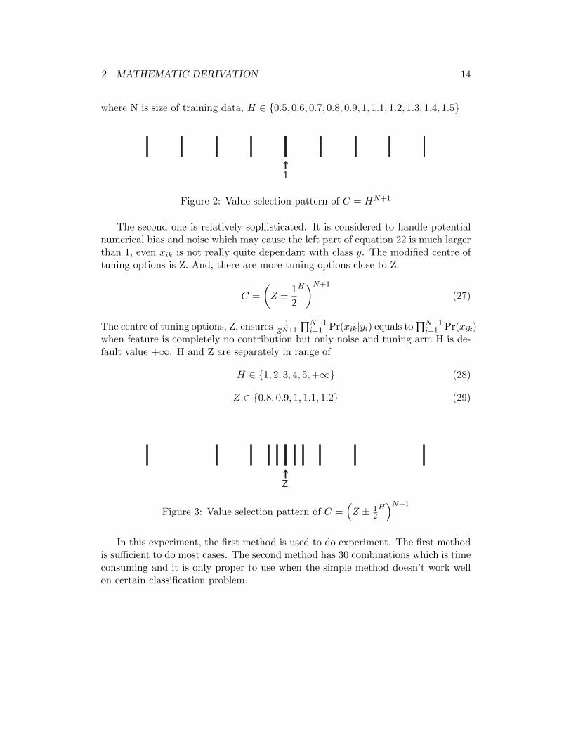
The second one is relatively sophisticated. It is considered to handle potentialnumerical bias and noise which may cause the left part of equation 22 is much largerthan 1, even xik is not really quite dependant with class y. The modified centre oftuning options is Z. And, there are more tuning options close to Z.

C =

(Z ± 1

2

H)N+1

(27)

The centre of tuning options, Z, ensures 1ZN+1

∏N+1i=1 Pr(xik|yi) equals to

∏N+1i=1 Pr(xik)

when feature is completely no contribution but only noise and tuning arm H is de-fault value +∞. H and Z are separately in range of

H ∈ {1, 2, 3, 4, 5,+∞} (28)

Z ∈ {0.8, 0.9, 1, 1.1, 1.2} (29)

Z

Figure 3: Value selection pattern of C =(Z ± 1

2

H)N+1

In this experiment, the first method is used to do experiment. The first methodis sufficient to do most cases. The second method has 30 combinations which is timeconsuming and it is only proper to use when the simple method doesn’t work wellon certain classification problem.

3 IMPLEMENTATION 15

3 Implementation

3.1 Formula in Practice

If we notice that there are too many multiplication in the function which may involveunderflow issue, it is obvious that our formula deducted in previous section is notready for implementing in programming language. So, log form is again used hereas equation 30 shown below:

log(Pr(y|~x,D)) ∝ log(Pr(y))×

(K∑k=1

log(G(k = 1) +G(k = 0))

)(30)

where G(k) = Pr(fk)∏N+1i=1 Pr(xik|yi, fk)

However, it is still insufficient to avoid underflow problem. When number oftraining data increasing, function G(k) tend to be to zero. Therefore, a muchsimple question similar to this one is considered: How to transform log(A+B)? Itturns out if it is changed into the form shown in equation 31, the underflow problemcan be solved.

log(A+B) = log(A) + log(B

A+ 1) if A > B (31)

Correspondingly, if value of G(k = 1) is much larger than that of G(k = 0),log(G(k = 1) +G(k = 0)) is very close to log(G(k = 1)). The property of equation31 is corresponding to automatic feature selection. If A represents that the featureis not selected and B represents that is selected, it is good to have results that eitherA or B, but not both or nothing.

3.2 WEKA API and Framework

In this work, I use Java an object-oriented programming language to implement theBMA algorithm under eclipse workbench. Since Java has the advantage of greatencapsulation property as Object-oriented programming language, I build severalpackage, classes and interfaces to meet OOP standard, which also give a good struc-ture for following explanation. Eclipse JAVA standard IDE is also used in thisproject to provide a better package management and version control. Furthermore,the environment of experiment is macbook pro 721 with 16GB memory which in-stalled mac OS 10.9 operating system. Note that Eclipse restrict memory usage bydefine eclipse.ini file in software package which I don’t change.

WEKA3, which contents a lots of classes of models, is a tool used in my projectto do final evaluation. Actually, WEKA is a complete suite of machine learning

3WEKA: Waikato Environment for Knowledge Analysis

3 IMPLEMENTATION 16

software which was written in Java. That means it is product that can directly beused in data analysis and data mining tasks4. It is worth mentioning that analysisalgorithm implementing codes of WEKA is a excellent way to learn machine learn-ing. This also proves the predictive model it provided is quite stable, popular andalso meet the requirement of being control algorithms. Note that we only importand use function Library of WEKA but not graphic interface.

The control group of the experiments consist of Logistic Regression, traditionalNaive bayes as well as support vector machine. Naive Bayes classifier is a in-builtWEKA class with pre-processing setting options, and SVM as well as Logistic Re-gression are abstracted from Liblinear package. To provide fair comparison, myimplementation is also made to be able to call those pre-processing functions as wellas setting options. Note that my implement of Bayesian model averaging is notbuilt on Naive bayes of WEKA, since some functions cannot be effectively extendfrom it. Therefore, A customized Gaussian Naive Bayes classifier has been built asbase of BMA. To ensure the experiment is complete reliable, I kept the customizedNaive Bayes classifier available and have it joined in comparing group as well. Itcan get exactly same results with Naive Bayes of WEKA in any circumstance.

Data sets I used in this project is from UCI data sets which have kinds ofclassification questions. But, considering capability of linear classifiers, only thosedataset which can be separated by linear classifier have been used. Additionally,since UCI data is in form of arff document, file reader function and storage class ofWEKA API are also hired.

3.3 Continuous Feature Handling

In previous subsections, the basic idea of Bayesian model averaging for naive bayesclassifier is introduced without considering continuous features which may signifi-cantly affect this algorithm. For handling continuous features, there are two mainway that normally being used for naive bayes. The first one is focusing on Gaus-sian assumption which assume that the values in continuous feature are followinggaussian distribution for each class. Another way is to discretize continuous valueby supervised clustering.

The traditional Naive Bayes classifier with gaussian distribution assumption iscalled gaussian naive bayes. This approach focuses on assuming continuous featuresare normal distributed. Theoretically, according to the Central limit theorem, it isvery natural to prove the rationality of assumption. However, as the theory implied,if the data set is very large, then it is good to apply this method. As contrast, if

4Actually, it is very common to see data mining introduction books which use WEKA as supporttheoretical practice such as ”Data mining: Practical machine learning tools and techniques”.

3 IMPLEMENTATION 17

the data set is not big enough, the accuracy of this method may be unsatisfiable.In this project, this method is applied for the Bayesian model averaging to handlenumerical features.

Since pursuing the precision of probability of value in Gaussian distribution iscostly, the probability of value is approximated by area of rectangular with desity asheight and a proper small value as width which is calculated based on σ as shown inequation. The expensive time consuming does not significantly impact Naive Bayesclassifier, but, for BMA, the cost is over the roof. Note that the

∏Ni=1 Pr(xik|yi, fk)

requires 2×N times calculation.

Pr(x) =

∫ x+ 12δ

−∞

1

σ√

2πe−

(z−µ)2

2σ2 dz −∫ x− 1

2δ

−∞

1

σ√

2πe−

(z−µ)2

2σ2 dz

≈ 1

σ√

2πe−

(x−µ)2

2σ2 × δ(32)

where δ =√σN and N is number of value added from training set.

−1 0 1 2 3 4 5 60

0.05

0.1

0.15

0.2

0.25

0.3

0.35

0.4

Data

Density

Attribute Distribution

Gaussian Assumption

Figure 4: Gaussian Distribution Assumption for Feature with Numerical Type

The missing value problem may cause gaussian BayesiaNaiven Model Averag-ing algorithm failure. To successful dealing with classification problem that containmissing value, the normally approach is to impute mean value of the gaussian dis-tribution in the missing place. However, this will be time consuming. What the

3 IMPLEMENTATION 18

weka does is just discard that feature in training process and ignore any of missingvalue in testing period which means it does classification with incomplete featureset. To make our implementation get exactly same preprocessing methods to meetbasic fairness requirement of comparison, I also used weka’s approach5.

The most popular approach to handle continuous value is discretisation whichgoal to separate continuous values into several discrete ranges. The advantage of thisapproach is that it performs very stable and normally provides better performance.There are several great way to implement this approach[Dougherty et al. 1995].However, it also has some shortcomings such as increasing time complexity. Theworst disadvantage for us is the feature discretised may not be always same withthe increasing of dataset. That makes our performance comparison of algorithmvery difficult to keep fairness, since the features in each algorithm may not same.The related implementation of this approach on BMA can be activated by usingparameter −D. But in the following experiment, it is not activated.

3.4 Robustness and Missing Value Handling

Since size of training data is always limited, it is impossible to guarantee the classifierwould never meet unseen feature values. To tolerate existence of new feature values,smoothing method has been applied in the algorithm to meet baseline robustnessrequirement. The smoothed estimator is following Dirichlet prior distribution asequation shown below. Normally, when l is set to 1, then this approach is calledas Laplace smoothing[M.Mitchell 2010]. Note that l is also hyper-parameter, but inthis work, we keep it to 1.

Pr(Xi = xij |Y = yk) =#D{Xi = xij

∧Y = yk}+ l

#D{Y = yk}+ lJ(33)

For numerical features, since we dropped missing value directly in training process,it is possible that one class may doesn’t contain any value at all. This means thereexist feature xi in class y that doesn’t follow normal distribution, since there is nomean and standard deviation. To handle this, a default baseline standard deviationhas been signed. Note that, mean is always zero, since the normal distribution weused here is after standardized.

Another risk that may cause algorithm fail is missing class label of trainingdataset or class label is real. The goal of this algorithm is to deal with classificationproblem, so A rejection preprocessing function has been applied to check and rejectregression problem as well as defective files.

5http://grepcode.com/file/repo1.maven.org/maven2/nz.ac.waikato.cms.weka/weka-stable/3.6.6/weka/classifiers/bayes/NaiveBayes.java

3 IMPLEMENTATION 19

3.5 Pseudocode and Explanation

In this subsection, A thorough explanation of this Bayesian Model Averaging im-plementation is described by using pseudo-code as well as corresponding analysis.As most of classification algorithm, this method also consist of training step andtesting step. Additionally, since this algorithm is implemented through Java, it isrelatively easy to use purely Object-oriented programming style to present a goodstructure. Note that the pseudo-code provided in this work also in the perspectiveof OOP. Algorithm 1 shown below is training part of BMA.

Algorithm 1 BayesianModelAveraingForNB

Require: Global V ariable : conditionalProbability[][] and prioriProbability1: function BuildClassifier(trainingset)2: PD← PreProcessing(trainingset) . Initial3: for i← 1,PD.NumberOfClasses + 1 do4: for j ← 1,PD.NumberOfAttributes do5: conditionalProbability[i][j].initialise() . Pr(xi|yj)6: end for7: end for8: prioriProbability.initialise() . Pr(y)9: for all inst ∈ PD do

10: for j ← 1, Inst.NumberOfAttributes do11: conditionalProbability[j][inst.class].AddValue(inst.attr(j).value)12: conditionalProbability[j][null].AddValue(inst.attr(j).value)13: end for14: prioriProbability.AddValue()15: end for16: conditionalProbability.CalculateProbability()17: prioriProbability.CalculateProbability()18: LogSumProcessing(PD)19: end function

Note that in line 3, there are N + 1 number of classes space has been initialized,since one of them is used to store Pr(x) that without any conditions. Correspond-ingly, in line 12, values are also added in to this storage without considering classinformation of that data.

The training procedure is quite similar with traditional Naive Bayes classifierexcept some additional functions and storages used to store extra information weneed. Before explaining those extra functions, It is must clear that the global vari-ables written in Algorithm 1 is not very global. It is actually private memberof classifier class, from which our final model initialised. Additionally, the build-Classifier function in class BMA of NB classifier demonstrates training process.

3 IMPLEMENTATION 20

LogSumProcessing() function shown in Algorithm 2 is a further processing of train-ing part, which gathering information about weights of models that our BayesianModel Averaging algorithm concerned mostly.


Require: Global V ariable : conditionalProbability[][] and prioriProbability1: function LogSumProcessing(PD)2: SumOfCondProbInLog.Initialize3: SumOfAveCondPorbinLog.Initialize4: for i← 1,PD.NumberOfAttributes do5: SumOfCondProbInLog[i]← SumLogCondProb(i);6: SumOfAveCondProbInLog[i]← SumAveLogCondProb(i);7: end for8: end function9: function SumLogCondProb(PD,Index) .

∏Ni=1 Pr(xik |yi, fk)&k = 1

10: Sum← 011: for i← 1,PD.NumberOfInstances do12: Temp← conditionalProbability[Index][PD[i].class].value(PD[i])13: Sum← Sum+ log(Temp)14: end for15: return Sum16: end function17: function SumAveLogCondProb(PD,Index) .

∏Ni=1 Pr(xik |yi, fk)&k = 0

18: Sum← 019: Sum← 020: for i← 1,PD.NumberOfInstances do21: Temp← conditionalProbability[Index][null].value(PD[i])22: Sum← Sum+ log(Temp)23: end for24: return Sum25: end function

In the implementation, Algorithm 2 is the final version that proved to be cor-rect among all attempting. According to all of description so far, it seems thatthe training part of BMA for NB is quite increasing the running time. However,the theoretical time complexity is only O(NF ), where N is the number of trainingsamples and F is number of features. Therefore, the time complexity for trainingprocess is linear for both N and F . the time complexity of testing process is O(CF ),where C is number of potential classes in the classification problem.

The following pseudo-code is the testing function of classifier class. Since thepriori probability Pr(fk = 0) equals to 1 and Pr(fk = 1) is effected by hyper pa-

3 IMPLEMENTATION 21

rameter, it doesn’t show in the testing part of algorithm explicitly. Note that thevalue of these two priori probability is re-ranked by discard common denominator.We only represent it by C in line 11.


Require: Global V ariable : (SC)SumOfCondProbInLog[], (P )prioriProbability(CP )conditionalProbability[][] and (SAC)SumOfAveCondProbInLog[]

1: function ClassifyInstance(instance)2: I← PreProcessing(instance) . Initial3: SelectedClassIndex = 14: MaxProbability = 05: for i← 1, I.NumberOfClasses do6: I.classIndex← i7: Prob[i]← log(P.class(i))8: for j ← 1, I.NumberOfAttributes do9: A← SC + log(CP [j][i].valueOf(I))

10: B ← SAC + log(Aveage(CP [j][i]))11: Prob[i] = Prob[i] + LogSum(A/C,B) . C is Hyper-Parameter12: end for13: if i = 1 then14: MaxProbability ← Prob[i]15: end if16: if i > 1 then17: if MaxProbability < Prob[i] then18: MaxProbability ← Prob[i]19: SelectedClassIndex← i20: end if21: end if22: end for23: returnSelectedClassIndex24: end function

The pseudo-code above is just for provide a clear description of this algorithm,which is without optimization. For obtaining faster running speed of testing process.We can explicitly compare SAC with SC and if SAC is larger then do nothing.Correspondingly, if SC is larger, then plus log(CP [j][i].valueOf(I)) on Prob[i].Therefore, the running time can be further reduced.

4 EXPERIMENT AND EVALUATION 22

4 Experiment and Evaluation

4.1 Cross-Validation

Cross-validation, also named rotation estimation, is a method that separate datasetinto several subsets to make some kinds of model analysis. Normally, cross-validationis not only used to get average error rate of classification but also is used to tunehyper-parameter of classifier to fit dataset.

There are several common types of cross-validation. The first one is called K-foldcross-validation, which randomly divide original sample set into subsets with equalsize. One of those subsets then be chosen as data used to test model and rest of thesubsets plays role of training data. This process repeats until every subset has beenchosen to be testing data. The results of k times evaluation then be averaged toproduce a single estimation. The second one called Repeated random sub-samplingvalidation. This method randomly splits the dataset into training data and testingdata and build model on training set to predict label of testing data. Then, evaluateresult. This process also repeat several times and the final evaluation is average ofall results. However, the difference between this method with K-fold is that theproportion of the testing data is not dependent on the number of iterations. Cross-validation implementations are not limited in these two methods.6

Random selected 10% of Dataset

First 10% of Training&Validating Dataset

Dataset

TestingTraining&

Validating

TrainingValidating

Figure 5: Random Resampling Cross Validation

In this work, A nested random resampling cross-validation model has been usedto do the evaluation task for two reasons. First of all, the 10-folds cross-validationis misleading when there are sparse data. Moreover, some task needs more than10 times experiments without effecting proportion of training and testing data sets.

62-fold cross-validation, leave-one-out cross-validation are commonly used in practice as well.


But 10-folds cross validation is still useful when dataset is large enough. Since thecomplete double level cross-validation would take very long time to do and doesn’tprovide much better hyper-parameter tuning results than fixed fold tuning7, tuninghyper parameter is implemented on fixed training and validating dataset withoutcrossing.

This method assumes the label of testing data set is unknown and it uses part ofknown dataset to adjust hyper-parameter, then apply it on whole training data setto predict label of testing data set. More detail about the cross-validation methodcan be find in the following algorithm.

Algorithm 4 Fast Cross Validation

Require: Classifier,Dataset1: function Random Cross-validation(Classifier, Dataset, numFold)2: Initial Result[numFold]3: for i← 1 to numFold do4: Dataset.Permutation(Seed) . Re−Arrange5: Testingset← RandomSelection(Dataset, 1/10)6: Trainingset← Dataset.RestOfInstances7: Classifier.hyperParameterTuning(Trainingset)8: Classifier.Train(Trainingset)9: Result[i]← Classifier.Test(Testingset)

10: end for11: Analysis(Result)12: end function13: function hyperParameterTuning(Sampleset)14: Initial Result[V alueOfHyperparameter.size] . Initial15: for h← 1 to V alueOfHyperparameter.size do16: Classifier.Setting(h) . Setting Parameter17: Folds[]← Sampleset.SplitToTenSets18: V alidingset← Folds[1]19: Trainingset← Sampleset.RestOfInstances20: Classifier.Train(Trainingset)21: Result[i]← Classifier.Test(Testingset)22: end for23: OptimalParameter ← getBestHyperParameter(Result)24: Classifier.Setting(OptimalParameter)25: end function

7use one fix fold as validating dataset and others as training dataset to tune hyper-parameterwithout crossing


4.2 UCI Dataset

Since the Bayesian Model Averaging for Naive Bayes algorithm we derived is ex-pected to be capable for general usage, kinds of classification data sets that fromdifferent research fields are required to test the algorithm. Furthermore, to analyzethe conditions that effect the performance of BMA, some feature of datasets is alsopreferred such as features number, data size missing value as well as how manytarget classes involved, etc.

Table 2 Experimental DataSets

FileName Features Data Size Classes Ratio Missing

anneal.arff 38 798 6 4.76% Yesautos.arff 26 205 7 12.68% Yesvote.arff 16 435 2 3.68% Yessick.arff 30 3772 2 0.80% Yescrx.arff 16 690 2 2.32% No

mushroom 22 8124 2 0.27% Yesheart-statlog.arff 13 270 2 4.81% No

segment.arff 19 2310 7 0.82% Nolabor.arff 16 57 2 28.07% Novowel.arff 14 990 11 1.41% No

audiology.arff 69 226 23 30.53% Yesiris.arff 5 150 3 3.33% Nozoo.arff 18 101 7 17.82% No

lymph.arff 19 148 4 12.84% Nosoybean.arff 35 683 19 5.12% Yes

balance-scale.arff 4 625 3 0.64% Noglass.arff 10 214 7 4.67% Noletter.arff 16 20000 26 0.08% No

hepatitis.arff 19 155 2 12.25% Nohaberman.arff 4 306 2 1.31% No

In this project, Datasets are abstracted from UCI datasets package. The abovetable shows some datasets used in the experiments, which can be handled by linearclassifiers with only one single target label.8 To discover some kinds of potentialpattern that can effect the performance of those algorithms including the BayesianModel Averaging implemented in this project, My experiment works on about 20

8Some classification problem with more than one label which represent that data is belong tomore than one classes.


datasets which include medical records, selling records and some classification prob-lem of sociology.

4.3 Control Group

The control group of experiments consists of SVM, Logistic Regression and Naive-Bayes classifiers. Naive Bayes classifier is the most representative generative linearclassification method and normally used as baseline classifier. Logistic Regressionrepresents classical discriminative linear classifier. And SVM is well known for itsgreat performance but relative lower speed. In this work, the BMA for NB classifieris expected to get better performance than Naive Bayes classifier and still maintainlinear time complexity and, of course, is also expected faster than SVM.

The SVM and Logistic Regression is abstracted from Liblinear API package9.The equation 34 is regularized error function, which is used by both SVM andLogistic Regression to optimize accuracy but avoid overfitting problem. Note thatthe specific error functions of those two classifiers are different[Fan et al. 2008].

min~w

1

2~wT ~w + C

l∑i=1

ξ (~w; ~xi; yi) (34)

Normally, as a tradition, regularization parameter is denoted as λ. But in Liblinearpackage, the λ is replaced by its reciprocal named C. Therefore,C is regarded aspenalty factor or cost factor. With increasing of C, the classifiers are more sensitiveto new dataset and even overfitting. However, A small value of C may not fit data,and bias of prediction with true value can be very big.

Another important parameter of Liblinear package is B, which refers to bias.Note that this bias is a constant which represent one additional dimension, but noterror bias. The following equation corresponds to separating hyperplane.

y (~x, ~w) =

K∑k=1

wkφk (~x) +B (35)

where φk is base function,~w is parameter vector and B is bias.

For Naive Bayes classifier, it is component of WEKA API and works withoutHyper-Parameter Tuning. However, it is still has some useful setting options. Themost important one is −D, which active supervised discretizing pre-processing.

9Liblinear: A library of Large Linear Classification is released by Machine Learning Groupof National Taiwan University. This package is widely used in machine learning practice, andcompatible with WEKA, R and other machine learning softwares


4.4 Experiment Results

In this sub section, a performance comparison of BMA for NB with other classifieris made. Since parameter tuning of SVM and LR is very time consuming, only 36parameter combination are provided for automatic tuning as shown bellow.

C ∈ {0.01, 0.1, 1, 10, 20, 100} (36)

B ∈ {0.01, 0.1, 1, 10, 20, 100} (37)

The following table gives 95% confidence interval of true error, in which out-standing classifier is bolded. Since the modification limitation of classifier fromWEKA, my implement of Bayesian Model Averaging is established on a customizednaive bayes classifier. To guarantee there is no doubt on performance bias of cus-tomised classifier with that of WEKA, both of their error rates are included in thistable and following tables.

Table 3 95% Confidence Interval for true error

Problems BMA CNB NB LR SVM

anneal 7.87±2.00 7.87±2.00 7.87±2.00 6.74±1.86 17.98±2.86? autos 30.00±7.13 40.00±7.62 40.00±7.62 25.00±6.74 55.00±7.74? vote 4.65±2.25 11.63±3.42 11.63±3.42 4.65±2.25 4.65±2.25? sick 6.37±0.89 7.69±0.97 7.69±0.97 2.65±0.58 4.51±0.75crx 23.19±3.58 23.19±3.58 23.19±3.58 18.84±3.32 21.74±3.50

? mushroom 1.35±0.29 3.82±0.47 3.82±0.47 2.96±0.42 4.06±0.49heartstat 7.41±3.55 7.41±3.55 7.41±3.55 18.52±5.27 11.11±4.26segment 23.81±1.97 23.81±1.97 23.81±1.97 10.82±1.44 14.72±1.64

labor 0.00±0.00 0.00±0.00 0.00±0.00 0.00±0.00 0.00±0.00? vowel 33.33±3.34 42.42±3.50 42.42±3.50 44.44±3.52 47.47±3.54

? audiology 22.73±6.21 27.27±6.60 27.27±6.60 9.09±4.26 13.64±5.09? iris 6.67±4.54 13.33±6.18 13.33±6.18 6.67±4.54 6.67±4.54zoo 0.00±0.00 0.00±0.00 0.00±0.00 0.00±0.00 0.00±0.00

lymph 7.14±4.72 7.14±4.72 7.14±4.72 14.29±6.41 14.29±6.41soybean 11.76±2.75 11.76±2.75 11.76±2.75 10.29±2.59 11.76±2.75balance 9.68±2.63 9.68±2.63 9.68±2.63 16.13±3.28 12.90±2.99

glass 52.38±7.61 52.38±7.61 52.38±7.61 33.33±7.18 47.62±7.61? letter 34.05±0.75 35.25±0.75 35.25±0.75 STUCK STUCK

hepatitis 26.67±7.91 26.67±7.91 26.67±7.91 60.00±8.77 46.67±8.93haberman 33.33±6.00 33.33±6.00 33.33±6.00 36.67±6.14 33.33±6.00

The classification problem letter consists of 20,000 data, which is a challengefor Logistic Regression and SVM to finish classification in relatively short time. In


this work, the threshold of running time is 10 minutes. They don’t finish runningin the limited time and are labeled to be stuck. According to the designer of theLiblinear package, this is caused by large assignment of bias B. However, small Bis not sufficient to get good prediction accuracy. It seems to be a time complexityand accuracy dilemma.

According to table 3, Bayesian Model Averaging for Naive Bayes classifier getseither better performance than Naive Bayes or gets equivalent performance with itsbase. It is because of the automatic feature selection mechanism of BMA for NB asshown in Figure 6.

0 5 10 15

0.6

0.7

0.8

0.9

Number Of Feature

Acc

ura

cy

vote.arff

BMANB

Figure 6: Example of Automatic Model Weighting and Feature Selection

With automatic feature selection mechanism of Bayesian Model Averaging, fea-tures which not really depend on label y are ignored and feature with great contri-bution for classification are boosted. Additionally, because of existence of the hyperparameter, models with relative higher dimension get extra cost. Therefore, theBayesian Model Averaging ignores some noise features and then gets overall betterperformance.

Since feature selection doesn’t guarantee getting better performance and caneven decrease prediction accuracy10, it is good to know that for which kinds of clas-

10For some classification problem, the feature set has already thoroughly chose and collected.Therefore, feature extraction maybe more useful than selection.


sification problem feature selection is good and then decide whether or not applyingfeature selection.

In natural language processing field, it is very important to do entity recognition,feature selection as well as dimension reduction, since there are so many useless orsimilar features which can decrease accuracy. Therefore, text classification problemsare good to test the affection of feature selection. In this work, a binary classifica-tion problem which is abstracted from 20 newsgroup dataset has been used to testthe affection of feature number on prediction accuracy as shown in Figure 7.

0 100 200 300 400 500 600 700 800 900 1,000 1,100

0.5

0.6

0.7

0.8

0.9

1

Number Of Features

Acc

ura

cy

News Group

BMANBLR

SVM

Figure 7: Accuracy based on number of Features

This plot is worked on 1000 data which selected from two categories of news. itis an exactly balanced dataset. The 1000 features are selected from 20,000 wordswith high frequency of occurrence after applied stop list checking. Note that thisplot is averaged on results from multiply runs with feature resampling.

After around 150 features selected, the BMA, SVM and Logistic Regression showsignificantly better performance than Naive Bayes classifier. Furthermore, the ac-curacy of BMA, SVM and Logistic Regression are also stablized earlier. It showsthat BMA has better noise resistant property.


To show whether training dataset size can significantly impact the accuracy ofnews classification task, the related experiment has made. This plot is generatedwhen classifiers perform on news group dataset with 2000 data and 500 selectedfeatures. The testing dataset which has 500 data is fix in each run. Note that thisplot is averaged on results from multiply runs with data resampling.

0 10 20 30 40 50 60 70 80 90 100

95

96

97

98

99

100

Percentile of Dataset with 2000 Data

Acc

ura

cy

News Group

BMANBLR

SVM

Figure 8: Accuracy based on size of Dataset

The experiment shows that the prediction accuracy is stable after enough train-ing data is used and further training is no significant affection.

The following is time consuming table which records running time of classifiersfor all of those classification problems. Note that this table generated without takinghyper parameter tuning time into account. In practice, hyper parameter tuning oc-cupies much more time then classifier training procedure itself. In this experiment,36 setting options are used for SVM and Logistic Regression, but they still can’tguarantee to provide relative reliable results for all of those classification problems.As contrast, even though no setting options are used to optimize performance ofBMA, it is sufficient to make sure the performance is not worse than baseline clas-sifier.


Table 4 Time Comsuming Table measured in µs

Problems BMA CNB NB LR SVM

anneal 709956 169878 151395 581915 2059308autos 106283 46622 66247 177798 1287179vote 11200 5836 7404 21812 33452sick 323999 94433 82246 426820 2487667crx 76626 24516 14912 64160 541535

mushroom 271375 81395 88018 1061161 5759504heart-statlog 36333 14071 7421 21932 216576

segment 588319 211444 156669 2611166 6703656labor 3726 1763 2119 4973 26152vowel 139689 48997 46199 579517 5329444

audiology 95783 13767 42654 170953 264345iris 4970 2167 2508 10140 119829zoo 6982 2806 3524 31512 219978

lymph 12320 5566 4678 21867 173912soybean 115032 17828 53516 572924 824965

balance-scale 25865 6602 5630 40782 530705glass 22901 9315 8075 50113 620718

hepatitis 8205 3313 3644 15664 127486haberman 7474 3370 2321 11180 153196

The combination of evidences above shows that the implementation of BMAbased on Naive Bayes can provide better prediction for some specific classificationproblem with relatively less time consuming such as vote,vowel and mushroom. Andeven if it can’t give better performance, it can still guarantee the accuracy is equalto baseline algorithm. through comparing the true error confidence interval tablewith experiment dataset table, we believe the accuracy improvement of BMA withrespect to Naive Bayes classifier is not related to number of features, number ofdataset, number of classes as well as missing values. The improvement is only re-lated to how many of features in that classification problem is trivial or just noise.

As previous discussed, the hyper parameter of this implementation of BMA forNB is C, which is further expressed as shown in equation 38.

C = HN+1 (38)

where N is training data size and H is tuned parameter.In this experiment,

H ∈ {0.5, 0.6, 0.7, 0.8, 0.9, 1, 1.1, 1.2, 1.3, 1.4, 1.5} (39)

.


The following plots shows the affection of tuning hyper parameter.

0 0.2 0.4 0.6 0.8 1 1.2 1.4 1.6

20

30

40

50

60

70

80

90

100

Hyper-Parameter Value

Acc

ura

cy

sickvote

mushroomaudiologyanneal

crxlymph

Figure 9: Example of Hyper Parameter Tuning Affection 1

With the increasing of the Hyper-parameter value, the accuracy of predictiongradually grows at first period. But after passing the peak, it declines normally veryfast. It is caused by over punishment of model with higher dimensions. The lefthand side which shown as straight line means there is no affection that brought byhyper parameter yet. And, the right hand looks like gradient descent and each ofthe descent corresponding the prediction accuracy provided by models with slightlyless features.


However, even though there exist peak or platform for some classification prob-lems, it is not guaranteed the hyper parameter with the best prediction accuracycan be selected by automatic hyper parameter tuning process in cross validation,because the validating dataset may not be able to represent the property of testingdataset as well as training dataset.

And, it is also worth to mention that the above cases is not always true, sincethe essence of this algorithm is based automatic feature selection. Therefore, if aclassification problem whose features all make contributions, tuning hyper parameterto punish models with relative more features can only get worse result. Thus, thereis no peak at all as shown below.

0 0.2 0.4 0.6 0.8 1 1.2 1.4 1.6

10

20

30

40

50

60

70

80

90

Hyper-Parameter Value

Acc

ura

cy

balance− scaleglass

soybeansegment

haberman

Figure 10: Example of Hyper Parameter Tuning Affection 2

5 CONCLUSION 33

5 Conclusion

This work is to implement a well-known model combination technology BayesianModel Averaging into the classic and robust classifier Naive Bayes. The motiva-tion is that, even though Bayesian model averaging is a commonly used approachto combine models and do automatic feature selection11, there are not much re-searches implementing it on Naive Bayes. In this work, we derive a new BMA forNaive Bayes classifier algorithm with new automatic feature selection mechanism.The time complexity of the algorithm is mathematically proved to be linear withrespect to both number of features and number of data. Then, the algorithm isimplemented through Java program and evaluated through several aspects.

The experiment results are quite near what we expected: the performance isbetter than original Naive Bayes algorithm and its time complexity is similar withNaive Bayes as well. The challenge is to improve this method to get better perfor-mance which is competitive with other linear classification models. According tothe experiment results, it is clear that the implementation is very competitive onseveral cases such as text classification. For some classification problem like vote.arffor sick.arff, performance of BMA for Naive Bayes classifier is much better than tra-ditional Naive Bayes classifier, and In other cases, however, the performances is justsame with Naive Bayes classifier. Furthermore, this algorithm is faster than SVMand Logistic Regression and, for some cases, it also provides better accuracy thanthem.

The possible usage of this classifier is for those classification problems whichinclude lots of useless features or noise features with relatively less dependence withclass label. Text classification problem in this experiment is proved to be a poten-tial field for which the classifier has its advantage, since automatic feature selectionmechanism of the BMA on NB can play a role.

Hyper parameter tuning is very critical for this classifier. It controls the cost ofhiring features for a model. However, because C is real number, its tuning rangeis very large, therefore, tuning every possible value of the hyper parameter C iscostly and almost impossible. To roughly adjust this parameter, exponential ad-justing point is used, which is HN+1, where N is number of training data andH ∈ 0.5, 0.6..1.5. The advantage of this method is it can significantly reduce theparameter tuning time. As contrast, it is possible to ’miss’ some crucial value whichmay increase the performance accuracy.

11some researchers are more likely to believe BMA is a feature selection tool rather than that ofmodel combination, since it tend to give ”the best” model too much weights(almost 20times bigger,even if there is only 1% difference in accuracy for Logistic Regression.)

5 CONCLUSION 34

The most difficult period in my work is the time that I struggle to adjust hyper-parameters automatically. The current solution is just a compromise between ac-curacy and time consuming. This compromise clearly limited the usage of thisclassifiers, since there is no guarantee to say this classifier can beat Naive Bayes inmost circumstance with relatively higher computational cost. So how to find valueof hyper parameters more efficiently will become the further work.

A APPENDIX 35

A Appendix

A.1 Notations

A.1.1 General Notations

1 BMA: Bayesian Model Averaging

2 NB: Naive Bayes

3 SVM: Support Vector Machine

4 LR: Logistic Regression

5 OOP: Object-oriented Programming

A.1.2 Notation In Equations

1 y: class label

2 ~x: descriptive attributes of a data sample, it is a vector

3 xi: descriptive attributes of data sample i in training data set

4 xik: descriptive attribute k of data sample i in data set

5 M : model sets

6 m: a single model

7 mk: the number k model in model set

8 mki : the number i feature in model k

9 F : model sets which is notated by feature selection perspective.

10 ~f feature set vector

11 fk: number k feature in explanation features. The value rank is in 0 and 1.

12 di: number i data sample in data set

Bibliography 36

Bibliography

Dougherty, J., Kohavi, R., and Sahami, M. 1995. Supervised and unsuper-vised discretization of continuous features. (p. 18)

Fan, R.-E., Chang, K.-W., Hsieh, C.-J., Wang, X.-R., and Lin, C.-J. 2008.Liblinear - a library for large linear classification. The Weka classifier works withversion 1.33 of LIBLINEAR. (p. 25)

Fung, P. C. G., Morstatter, F., and Liu, H. 2011. Feature selection strat-egy in text classification. In Advances in Knowledge Discovery and Data Mining ,pp. 26–37. Springer. (pp. 5, 8)

Godec, M., Leistner, C., Saffari, A., and Bischof, H. 2010. On-linerandom naive bayes for tracking. In Pattern Recognition (ICPR), 2010 20th In-ternational Conference on (2010), pp. 3545–3548. IEEE. (p. 5)

Hoeting, J. A., Madigan, D., Raftery, A. E., and Volinsky, C. T. 1999.Bayesian model averaging: A tutorial. (p. 5)

M.Mitchell, T. 2010. Generative and discriminative classifier: Naive bayes andlogistic regression. (p. 18)

Ng, A. Cs229 lecture notes part IV: Generalized linear models.

Ng, A. Cs229 lecture notes part V: Support Vector Machines.

Ng, A. Y. and Jordan, M. I. 2002. On discriminative vs. generative classifiers:A comparison of logistic regression and naive bayes.

Raftery, A. E., Madigan, D., and Hoeting, J. A. 1997. Bayesian modelaveraging for linear regression models. Journal of the American Statistical Asso-ciation 92, 437, 179–191. (p. 5)

Yuan, Z. and Yang, Y. 2004. Combining linear regression models:when andhow?

Zhang, H. 2004. The optimality of naive bayes. A A 1, 2, 3. (p. 8)

bayesian model averaging for improving performance of the ... · bayesian model averaging for...

Documents