bayesian learning

CS 5751 Machine Learning

Chapter 6 Bayesian Learning 1

Bayesian Learning• Bayes Theorem• MAP, ML hypotheses• MAP learners• Minimum description length principle• Bayes optimal classifier• Naïve Bayes learner• Bayesian belief networks



Two Roles for Bayesian MethodsProvide practical learning algorithms:• Naïve Bayes learning• Bayesian belief network learning• Combine prior knowledge (prior probabilities)

with observed data

Requires prior probabilities:• Provides useful conceptual framework:• Provides “gold standard” for evaluating other

learning algorithms• Additional insight into Occam’s razor



Bayes Theorem

• P(h) = prior probability of hypothesis h• P(D) = prior probability of training data D• P(h|D) = probability of h given D• P(D|h) = probability of D given h

)(

)()|()|(

DP

hPhDPDhP



Choosing Hypotheses

Generally want the most probable hypothesis given the training data

Maximum a posteriori hypothesis hMAP:

If we assume P(hi)=P(hj) then can further simplify, and choose the Maximum likelihood (ML) hypothesis

)(

)()|()|(

DP

hPhDPDhP

)()|(maxarg

)(

)()|(maxarg

)|(maxarg

hPhDP

DP

hPhDP

DhPh

Hh

Hh

HhMAP

)|(maxarg iHh

ML hDPhi



Bayes TheoremDoes patient have cancer or not?

A patient takes a lab test and the result comes back positive. The test returns a correct positive result in only 98% of the cases in which the disease is actually present, and a correct negative result in only 97% of the cases in which the disease is not present. Furthermore, 0.8% of the entire population have this cancer.

P(cancer) = P(cancer) =

P(+|cancer) = P(-|cancer) =

P(+|cancer) = P(-|cancer) =

P(cancer|+) =

P(cancer|+) =



Some Formulas for Probabilities• Product rule: probability P(A B) of a conjunction

of two events A and B:

P(A B) = P(A|B)P(B) = P(B|A)P(A)• Sum rule: probability of disjunction of two events

A and B:

P(A B) = P(A) + P(B) - P(A B)

• Theorem of total probability: if events A1,…,An

are mutually exclusive with , then

n

i iAP1

1)(

n

iii APABPBP

1

)()|()(



Brute Force MAP Hypothesis Learner

1. For each hypothesis h in H, calculate the posterior probability

2. Output the hypothesis hMAP with the highest posterior probability

)(

)()|()|(

DP

hPhDPDhP

)|(maxarg DhPhHh

MAP



Relation to Concept LearningConsider our usual concept learning task• instance space X, hypothesis space H, training

examples D• consider the FindS learning algorithm (outputs

most specific hypothesis from the version space VSH,D)

What would Bayes rule produce as the MAP hypothesis?

Does FindS output a MAP hypothesis?



Relation to Concept LearningAssume fixed set of instances (x1,…,xm)

Assume D is the set of classifications

D = (c(x1),…,c(xm))

Choose P(D|h):

• P(D|h) = 1 if h consistent with D

• P(D|h) = 0 otherwise

Choose P(h) to be uniform distribution

• P(h) = 1/|H| for all h in H

Then

otherwise0

with consistent is if)|(

1 DhDhP H,DVS



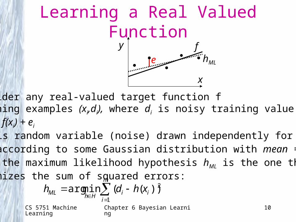
Learning a Real Valued Functionf

hML

y

x

e

Consider any real-valued target function fTraining examples (xi,di), where di is noisy training value• di = f(xi) + ei

• ei is random variable (noise) drawn independently for each xi according to some Gaussian distribution with mean = 0Then the maximum likelihood hypothesis hML is the one thatminimizes the sum of squared errors:

m

iii

HhML xhdh

1

2))((minarg



Learning a Real Valued Function

2

2

2

2

2

12

1

)(minarg

)(maxarg

σ

)(

2

1maxarg

σ

)(

2

1

πσ2

1lnmaxarg

... instead thisof log natural Maximizeπσ2

1maxarg

)|(maxarg

)|(maxarg

2

σ)(

21

iiHh

iiHh

ii

Hh

ii

HhML

m

iHh

m

ii

Hh

HhML

xhd

xhd

xhd

xhdh

e

hdp

hDph

ixhid



Minimum Description Length PrincipleOccam’s razor: prefer the shortest hypothesisMDL: prefer the hypothesis h that minimizes

where LC(x) is the description length of x under encoding C

Example:• H = decision trees, D = training data labels• LC1(h) is # bits to describe tree h• LC2(D|h) is #bits to describe D given h

– Note LC2 (D|h) = 0 if examples classified perfectly by h. Need only describe exceptions

• Hence hMDL trades off tree size for training errors

)|()(minarg 21 hDLhLh CCHh

MDL



Minimum Description Length Principle

Interesting fact from information theory:The optimal (shortest expected length) code for an

event with probability p is log2p bits.So interpret (1):

-log2P(h) is the length of h under optimal code

-log2P(D|h) is length of D given h in optimal code

prefer the hypothesis that minimizes length(h)+length(misclassifications)

(1) )(log)|(log minarg

)(log)|(log maxarg

)()|(maxarg

22

22

hPhDP

hPhDP

hPhDPh

Hh

Hh

HhMAP



Bayes Optimal ClassifierBayes optimal classification

Example:

P(h1|D)=.4, P(-|h1)=0, P(+|h1)=1

P(h2|D)=.3, P(-|h2)=1, P(+|h2)=0

P(h3|D)=.3, P(-|h3)=1, P(+|h3)=0

therefore

and

Hhiij

Vvi

j

DhPhvP )|()|(maxarg

- )|()|(maxarg

Hhiij

Vvi

j

DhPhvP

Hhii

Hhii

i

i

DhPhP

DhPhP

6.)|()|(

4.)|()|(



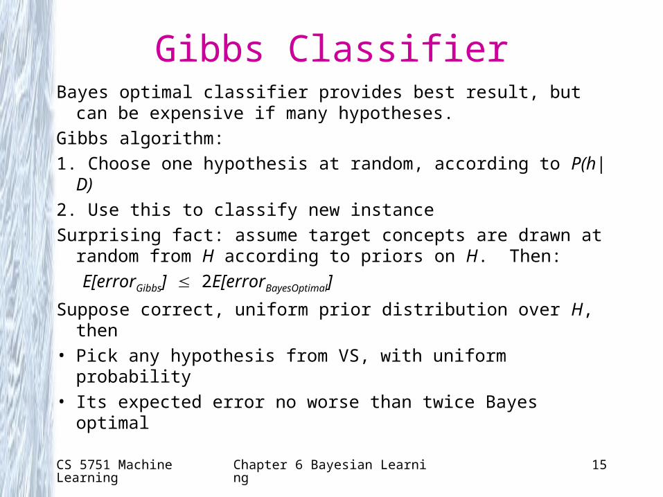
Gibbs ClassifierBayes optimal classifier provides best result, but can be

expensive if many hypotheses.

Gibbs algorithm:

1. Choose one hypothesis at random, according to P(h|D)

2. Use this to classify new instance

Surprising fact: assume target concepts are drawn at random from H according to priors on H. Then:

E[errorGibbs] 2E[errorBayesOptimal]

Suppose correct, uniform prior distribution over H, then

• Pick any hypothesis from VS, with uniform probability

• Its expected error no worse than twice Bayes optimal



Naïve Bayes ClassifierAlong with decision trees, neural networks, nearest

neighor, one of the most practical learning methods.

When to use• Moderate or large training set available• Attributes that describe instances are conditionally

independent given classification

Successful applications:• Diagnosis• Classifying text documents



Naïve Bayes ClassifierAssume target function f: XV, where each instance

x described by attributed (a1,a2,…,an).Most probable value of f(x) is:

Naïve Bayes assumption:

which givesNaïve Bayes classifier:

)()|,...,,(maxarg

),...,,(

)()|,...,,(maxarg

),...,,|(maxarg

21

21

21

21

jjnVv

n

jjn

Vv

njVv

MAP

vPvaaaP

aaaP

vPvaaaP

aaavPv

j

j

j

)|()|,...,,( 21 ji

ijn vaPvaaaP

)|()(maxarg ji

ijVv

NB vaPvPvj



Naïve Bayes Algorithm

)|v(aP) (vPv

x

)|vP(a)|v(aP

aa

)P(v)(vP

v

examples

xajij

VvNB

jiji

i

jj

j

ij

ˆˆmaxarg

)e(ew_InstancClassify_N

estimate ˆ

attributeeach of valueattributeeach For

estimate ˆ

t valueeach targeFor

)s_Learn(Naive_Baye



Naïve Bayes Subtleties1. Conditional independence assumption is often

violated

• … but it works surprisingly well anyway. Note that you do not need estimated posteriors to be correct; need only that

• see Domingos & Pazzani (1996) for analysis• Naïve Bayes posteriors often unrealistically close

to 1 or 0

)|()|,...,,( 21 ji

ijn vaPvaaaP

)|,...,()(maxarg)|(ˆ)(ˆmaxarg 1 jnjVv

ji

ijVv

vaaPvPvaPvPjj



Naïve Bayes Subtleties2. What if none of the training instances with target

value vj have attribute value ai? Then

Typical solution is Bayesian estimate for

• n is number of training examples for which v=vj • nc is number of examples for which v=vj and a=ai

• p is prior estimate for • m is weight given to prior (i.e., number of “virtual”

examples)

0)|(ˆ)(ˆ

... and ,0)|(ˆ

ji

ij

ji

vaPvP

vaP

mn

mpnvaP c

ji

)|(ˆ

)|(ˆji vaP

)|(ˆji vaP



Bayesian Belief NetworksInteresting because• Naïve Bayes assumption of conditional

independence is too restrictive• But it is intractable without some such

assumptions…• Bayesian belief networks describe conditional

independence among subsets of variables• allows combing prior knowledge about

(in)dependence among variables with observed training data

• (also called Bayes Nets)



Conditional IndependenceDefinition: X is conditionally independent of Y given

Z if the probability distribution governing X is independent of the value of Y given the value of Z; that is, if

more compactly we write P(X|Y,Z) = P(X|Z)

Example: Thunder is conditionally independent of Rain given LightningP(Thunder|Rain,Lightning)=P(Thunder|Lightning)

Naïve Bayes uses conditional ind. to justifyP(X,Y|Z)=P(X|Y,Z)P(Y|Z) =P(X|Z)P(Y|Z)

)|(),|(),,( kikjikji zZxXPzZyYxXPzyx



Bayesian Belief Network

Storm

Lightning Campfire

BusTourGroup

Thunder ForestFire

S,B S,¬B ¬S,B ¬S,¬B C 0.4 0.1 0.8 0.2¬C 0.6 0.9 0.2 0.8

Campfire

Network represents a set of conditional independence assumptions• Each node is asserted to be conditionally independent of its nondescendants, given its immediate predecessors• Directed acyclic graph



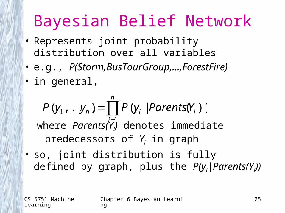
Bayesian Belief Network• Represents joint probability distribution over all

variables• e.g., P(Storm,BusTourGroup,…,ForestFire)• in general,

where Parents(Yi) denotes immediate predecessors of Yi in graph

• so, joint distribution is fully defined by graph, plus the P(yi|Parents(Yi))

n

iiin YParentsyPyyP

11 ))(|(),...,(



Inference in Bayesian NetworksHow can one infer the (probabilities of) values of

one or more network variables, given observed values of others?

• Bayes net contains all information needed• If only one variable with unknown value, easy to

infer it• In general case, problem is NP hardIn practice, can succeed in many cases• Exact inference methods work well for some

network structures• Monte Carlo methods “simulate” the network

randomly to calculate approximate solutions



Learning of Bayesian NetworksSeveral variants of this learning task• Network structure might be known or unknown• Training examples might provide values of all

network variables, or just some

If structure known and observe all variables• Then it is easy as training a Naïve Bayes classifier



Learning Bayes NetSuppose structure known, variables partially

observable

e.g., observe ForestFire, Storm, BusTourGroup, Thunder, but not Lightning, Campfire, …

• Similar to training neural network with hidden units

• In fact, can learn network conditional probability tables using gradient ascent!

• Converge to network h that (locally) maximizes P(D|h)



Gradient Ascent for Bayes NetsLet wijk denote one entry in the conditional

probability table for variable Yi in the network

wijk =P(Yi=yij|Parents(Yi)=the list uik of values)

e.g., if Yi = Campfire, then uik might be (Storm=T, BusTourGroup=F)

Perform gradient ascent by repeatedly

1. Update all wijk using training data D

2. Then renormalize the wijk to assure

Dd ijk

ikijhijkijk w

duyPww

)|,(η

j ijkijk ww 1 0 , 1



Summary of Bayes Belief Networks• Combine prior knowledge with observed data• Impact of prior knowledge (when correct!) is to

lower the sample complexity• Active research area

– Extend from Boolean to real-valued variables– Parameterized distributions instead of tables– Extend to first-order instead of propositional

systems– More effective inference methods

bayesian learning

Documents