bayesian inversion - joint inversions in geophysics · bayesian inversion • main credits: –...

Bayesian inversion •  Main Credits:

–  Inverse problem Theory,Tarantola, 2005 –  Parameter Estimation and inverse problems, R. Aster et al., 2013 –  Théorie de l’information (problèmes inverse & traitement du signal) Lecture by D. Gibert and F. Lopez, IPGP, 2013

(http://www.ipgp.fr/~gibert/Information_Theory_Files/) (many slides borrowed from this source)

Olivier Coutant, seismology group,

ISTerre Laboratory, Grenoble University

Prac%ce: )p://ist-‐)p.ujf-‐grenoble.fr/users/coutanto/JIG.zip

Plan 1.  Introduction to Bayesian inversion 2.  Bayesian solution of the inverse problem

1.  Basic examples

3.  How to find the solution of the Bayesian inversion 1.  deterministic or stochastic

4.  The deterministic approach 1.  Linear and non linear 2.  More on regularization 3.  Resolution operator 4.  Joint inversion (e.g seismic and gravity)

5.  A practical case: seismic and gravity on a volcano

Bayesian inversion We saw this morning the inversion of linear problem:

data = Model x parameter ó

d1d2...dN

⎡

⎣

⎢⎢⎢⎢⎢

⎤

⎦

⎥⎥⎥⎥⎥

=Mij

⎡

⎣

⎢⎢⎢⎢

⎤

⎦

⎥⎥⎥⎥.

p1p2...pM

⎡

⎣

⎢⎢⎢⎢⎢

⎤

⎦

⎥⎥⎥⎥⎥

d =M p

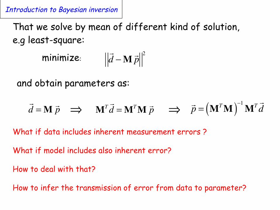
That we solve by mean of different kind of solution, e.g least-square:

d −M p

2

MTd =MTM p

d =M p

p = MTM( )−1MTd⇒ ⇒

minimize:

and obtain parameters as:

What if data includes inherent measurement errors ? What if model includes also inherent error? How to deal with that? How to infer the transmission of error from data to parameter?

Introduction to Bayesian inversion

Data with errors: d =dtrue+ εd Model with error: M=Mtrue+ εm M and d may be treated as statistical quantities given the statistics of the error ε: They are random variables with a given density of probability p(x) : defined by different moments of increasing order: - Expectation (mean) = - Variance = …

P(x ∈I ) = p(x)I∫ dx

E(x) = x.p(x)I∫ dx

Var(x) = (x − E(x))2 p(x)I∫ dx


What if we have an a priori knowledge about parameters? « There is a good chance that the earthquake is not located in the air, neither in the sea ; most likely in Ubaye beneath Barcelonnette » The Bayesian approach gives a good formalism to introduce: -  A priori knowledge on parameters -  Description of data and model errors -  To deal with non deterministic or non exact

direct model and coupling


Basic concept is both simple and very powerful: •  Probability (A and B) = Probability (B and A): P(A,B)=P(B,A) •  P(A,B) = Probability(A) x Probability (B with A realized): P(A,B)=P(A)P(B|A) •  P(B,A) = Probability(B) x Probability (A with B realized): P(A,B)=P(A)P(B|A) •  P(A) = Σ P(A|B) P(B) and P(B) = Σ P(B|A) P(A)

Bayes formula: P(A)P(B|A)=P(B)P(A|B) Let us call A event the data, and B event the parameter or model, then:

Posterior Probability on model

Prior Probability on model

Data likelyhood knowing the model

Bayesian solution of the inverse problem

P(B | A) = P(B)× P(A | B)P(A | B)P(B)∑

17 sept. 2012 -- Lecture 2 Information theory - D. Gibert - Year 2012-2013 5

Bayesian solution of inverse problems

Practical issues to obtain the Bayesian posterior probability:

P(B|A) = P(B) x P(A|B) ∫P(A,B)dB

The data likelihood for model B – P(A|B) – is obtained by computing the probability for the data to be actually observed if model B is the true model.

P(A|B) is a probability because:● the data contain errors and there is some probability that the data depart

from the model prediction.● the relationship giving the data from the model – the so-called forward

problem – may be imprecise or fundamentally of a probabilistic nature like in quantum mechanics (but not only).

P(A|B) is what will be called the “forward problem”

P(B | A) = P(B)× P(A | B)P(A | B)P(B)∑

Bayesian solution to inverse problem

Earthquake location problem: knowing seismic arrival times (P, S, Pg, Pn)

è invert for source location (x,y,z)

Bayesian solution to inverse problem: more on data and model error

homogeneous gradient Gradient + 2 layers

•  Systematic bias between these three models •  Model 1 introduce systematic error on Pn (refracted waves) data type



Practical issues to obtain the Bayesian posterior probability:

P(B|A) = P(B) x P(A|B) ∫P(A,B)dB

The prior probability for model B – P(B) – represents the amount of information available BEFORE performing the Bayesian inversion.

P(B) may be obtained or applied by:● using the posterior probability of another, previously solved, inverse

problem.● defining the parameter space in order to restrict it to the a priori

probable values of the parameters.

Finally, the Bayesian solution is extented to the continuous case:

P(B | A) = P(B)× P(A | B)P(A | B)P(B)∑

ρ(m | d) = ρ(m)× ρ(d |m)ρ(d |m)ρ(m)dm∫


m: model d: data


Introduction

The solution of a given inverse problem may constitute the prior information of another inverse problem.




Probabilistic forward problem: deterministic physical law and exact data

B (model)

A (data)

B1

P(A|B)

A1

P(A2|B1) = 0P(A1|B1) = 1

A2




Probabilistic forward problem: fuzzy physical law

B (model)

A (data)

B1

P(A|B)

A1

P(A2|B1)P(A1|B1)

A2




Probabilistic forward problem: deterministic physical law and imprecise data

B (model)

A (data)

B1

P(A|B)

A1

P(A2|B1)P(A1|B1)

A2


Remarks The direct problem may be more or less difficult to solve either analytically or numerically. The resolution of the forward problem often represents a great deal of work. The relationship between data and parameters may be linear: -  For instance gravity anomaly is doubled if density is multiplied by a factor of 2 The relationship betwwen datat and parameters is often non-linear: -  Gravity anomaly is not divided by 2 if the depth of the causative source is

multiplied by 2

The forward problem often has a unique solution -  A given geological structure produces one gravity anomaly

A remarkable property of inverse problems is that they generally have multiple acceptable solutions But, different geological structures may produce the same, or very comparable gravity anomaly

J

J

Gravity measurement from point Jg1

solve the inverse problem for a single measurement and a single parameter

•  We want to solve:

•  The theore%cal rela%on giving the ver%cal gravita%onal field is :

•  We assume here that the measurement is above the tunnel, that we know the radius, the density, and seek only for the depth

ρ(m | d) = ρ(m)ρ(d |m)ρ(d)

= ρ(m)ρ(d |m)ρ(m)ρ(d |m)dm∫

gz (x) =2π .G.ρ.rt

2.zt(x − xt )

2 + zz2

Example

•  The relation reduces to : with α=-1018.84. In our problem we measure g=-58.96 µgal;

ρ=2700kg/m3 and rt=3m

•  And the Bayes relation to be solve is

•  Let assume that the measurement g is subject to a Gaussian error with respect to the true value:

gz (zt ) =αzt

p(g | gtrue )∝ e−g−gtrue( )22σ g

2

ρ(zt | g) =ρ(zt )ρ(g | zt )ρ(g)ρ(g | zt )dzt∫

Example

•  And that the a priori function on the parameter is : zmin < zt <zmax

•  Then the solution of the inversion is

ρ(zt ) =1Δz

Πzt − zmoy

Δz⎛⎝⎜

⎞⎠⎟

ρ(zt | g) =Π

zt − zmoyΔz

⎛⎝⎜

⎞⎠⎟. e

−g−gtrue( )22σ g

2

e−g−gtrue( )22σ g

2

zmin

zmax∫ dzt

=Π

zt − zmoyΔz

⎛⎝⎜

⎞⎠⎟. e

−g−α

zt

⎛⎝⎜

⎞⎠⎟

2

2σ g2

e−g−gtrue( )22σ g

2

zmin

zmax∫ dzt

Example

Example


Example

Find the posterior probability of the tunnel depth. The prior probability is non-uniform and a single data (δg1) is used.

δg1


Example

Find the posterior probability of the tunnel depth. The prior probability is uniform and a two data (δg1 and δg2) are used.

δg1 δg2


Example

Find the posterior probability of the tunnel depth. The prior probability is uniform and a single data (δg2) is used.

δg2


Example

δg1

Find the posterior probability of both depth and horizontal position of the tunnel from a single data. Prior probability is uniform.


Example

δg1

Find the posterior probability of both depth and horizontal position of the tunnel from two data. Prior probability is uniform.

δg2

How to solve a Bayesian inversion?

1.  Find the maximum likelihood (ie: find the maximum of the a posteriori probability distribution)

ó a cost function ó optimization problem, deterministic approach

2.  Estimate the a posteriori expectation for y (mean value)

ρ(m | d) = ρ(m)ρ(d |m)ρ(m)ρ(d |m)dm∫

max m (ρ(m | d))

yρ(y | x)∫ dy

Deterministic approaches

3.  Explore the a posteriori density probability ρ(m|d) by a numerical approach «stochastic sampling»

- Metropolis-Hasting ( Richards Hobbs talk ) - Gibbs sampling; nested sampling - simulated annealing; genetic algorithm

4.  Model the a posteriori density by mean of analytical

representation:

–  Laplace approximation (Gaussian probability); –  Variational Bayesian methods ( see www.variational-bayes.org)

How to solve a Bayesian inversion?

Stochastic approaches

Deterministic approach (cf example solved above)

We assume a known density probability distribution for •  a priori density on parameters ρ(m) •  forward problem ρ(d|m) And solve for the maximum likelihood In practical we mostly consider “Gaussian” type density distribution:

ρ(m) = e−12m−mprior( )TCM

−1 m−mprior( )

ρ(d |m) = e−12g(m )−d( )TCd−1 g(m )−d( )

The Bayes formula becomes: where g(m) is a general non linear relation between data and model, mprior is our a priori hypothesis on the model. Cm and Cd are covariance matrices on the model and the data:

ρ(m | d)∝ e−12g(m )−d( )TCd−1 g(m )−d( ) −1

2m−mprior( )TCM

−1 m−mprior( )

Cm =

σ m12 . . .

. . Cji = Cij .

. Cij σ mj

2 .

. . . .

⎡

⎣

⎢⎢⎢⎢⎢⎢

⎤

⎦

⎥⎥⎥⎥⎥⎥

Deterministic approach

In the linear case: g(m) = G.m, it reduces to: which can also be written as a function of the “maximum of likelihood” estimator : which maximizes ρ(m|d), or equivalently minimizes:

ρ(m | d) = e−12

G .m−d( )TCd−1 G .m−d( ) + m−mprior( )TCm−1 m−mprior( ){ }

ρ(m | d) = e−12

m−m̂( )TCM '−1 m−m̂( ){ }

m̂

G .m−d( )T Cd

−1G .m−d( ) + m−mprior( )T CM

−1m−mprior( )

CM = GTCd−1G+Cm

−1( )−1

Deterministic approach, linear case

a posteri covariance on m

And the solution is (model space): (recall the least square solution) or (data space): that again minimizes

Deterministic approach, linear case

m̂ = mprior + (GTCd

-1G +Cm-1 )-1GTCd

-1 d −G.mprior( )

m̂ = mprior +CmGT(GTCmG+Cd )

-1 d −G.mprior( )

m̂ = (GTG)-1GTd

G .m−d Cd

2+ m−mprior Cm

2

For the non linear case, we wish to find that minimizes: We are now back to optimization iterative procedures. The solution using a quasi-newton method for instance is (Tarantola, 2005):

Deterministic approach, non-linear case

g(m )−d Cd

2+ m−mprior Cm

2

m̂

mn+1 = mn + µn (GnTCd

-1Gn +Cm-1 )-1 Gn

TCd-1 dn − d( ) +Cm-1 (mn −mprior )( )

Deterministic approach pro and con: -  easy to program -  flexible to fix a priori constraint on model -  Can fall in secondary minima -  Not suited for large scale problems

More on regularization

Back to least square problem: with solution: If G and hence GTG is ill-conditioned, or the system is under determined, or not unique or,…, the above linear system may not be solved and we need to regularize the system, ex SVD solution, …, or damped least square (Levenberg Marquardt) : which minimizes: Let’s compare our Bayesian deterministic solution to the LS solution using regularization techniques (Tikhonov)

m̂ = (GTG)-1GTd

m̂ = (GTG + λId )-1GTd

G .m−d2+ λ

2m

2

d =Gm

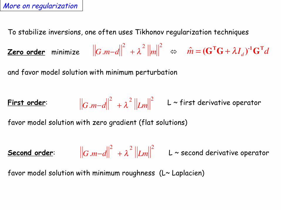
To stabilize inversions, one often uses Tikhonov regularization techniques Zero order minimize ó and favor model solution with minimum perturbation First order: L ~ first derivative operator favor model solution with zero gradient (flat solutions) Second order: L ~ second derivative operator favor model solution with minimum roughness (L~ Laplacien)


G .m−d2+ λ

2m

2m̂ = (GTG + λId )

-1GTd

G .m−d2+ λ

2Lm

2

G .m−d2+ λ

2Lm

2

How does Bayesian inversions compares to Tikhonov regularization? One minimizes: The operator acting on the model is the inverse of the covariance matrix.. In 1D, a covariance matrix is strictly equivalent to a smoothing or convolution operator: Cm s ó f*s where s is a signal and f filter impulse response


G .m−d2+ (m − mprior )

TCm

−1(m − mprior )

Cm−1

Cm=

⎡

⎣

⎢⎢⎢⎢

⎤

⎦

⎥⎥⎥⎥

Δ : Correla%on distance

Cm-1 is thus the reciprocal filter (i.e a highpass filter)

If we chose a covariance matrix with an exponential shape: Its Fourier tranform ó (k=wavenumber) The reciprocal filter (i.e Cm

-1) is By comparison, the second order tikhonov regularization operator is (Laplacien ) The bayesian inversion regularization operator is then a high pass filter with a characteristic length


e− i− j

Δ

e− xΔ 2Δ

1+ k2Δ2

1+ k2Δ2

2Δ

k2 ∂2

∂x2

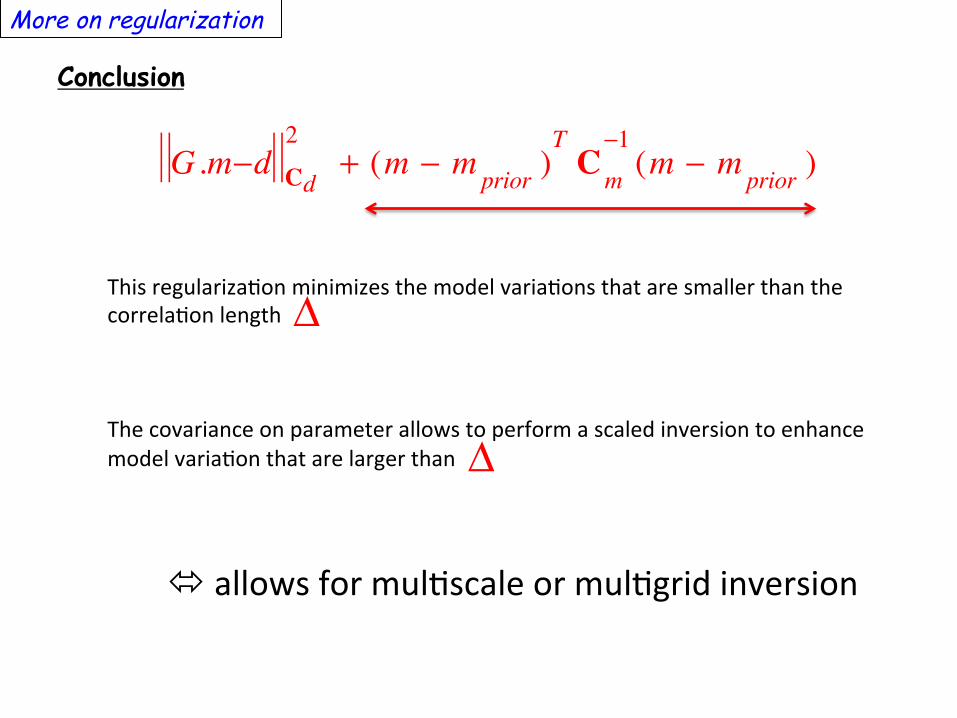
Conclusion


G .m−d Cd

2+ (m − mprior )

TCm

−1(m − mprior )

This regulariza%on minimizes the model varia%ons that are smaller than the correla%on length The covariance on parameter allows to perform a scaled inversion to enhance model varia%on that are larger than

ó allows for mul%scale or mul%grid inversion

Δ

Δ

Other regularizations: Total variation, minimize: where L=gradient operator => enhance sharp variations

Sparsity regularization, minimize: => maximize the number of null parameter


G .m−d2+ λ

2Lm

G .m−d2+ λ

2m

Resolution operator

It yields some insight on how well a parameter is resolved, and if neighbor solution are correlated or independent. For the bayesian, linear case, the resolution operator takes the form: and where is the a posteriori covariance matrix and the inverse a priori covariance matrix

R = I− CMCM−1

CM CM

−1

m̂ = Rmtrue

20000 40000 600000

0.02

Indices of model parameters(or column of the resolution matrix)

resolution matrix row for a parameter at 2 km depth(a)

(b)

0

0.004resolution lengths

(c)

630 635 640 645 650 655

0

8

Z U

TM (k

m)

X UTM (km)

(d)

0 0.005 0.01 0.015

0

4

8

Z U

TM (k

m)(e)

Parameter at 2 km depthAll indices of the line,QGLFHV�DORQJ�[ïD[LV,QGLFHV�DORQJ�\ïD[LV,QGLFHV�DORQJ�]ïD[LVParameter at 4 km depthParameter at 6 km depthNodes of density grid

diagonal term

Resolution along horizontal pro!le A-B

Resolution along vertical pro!le C-D

A BC

D

Resolution operator (Barnoud et al., 2015)

20000 40000 600000

0.02

Indices of model parameters(or column of the resolution matrix)

resolution matrix row for a parameter at 2 km depth(a)

(b)

0

0.004resolution lengths

(c)

630 635 640 645 650 655

0

8

Z U

TM (k

m)

X UTM (km)

(d)

0 0.005 0.01 0.015

0

4

8

Z U

TM (k

m)(e)

Parameter at 2 km depthAll indices of the line,QGLFHV�DORQJ�[ïD[LV,QGLFHV�DORQJ�\ïD[LV,QGLFHV�DORQJ�]ïD[LVParameter at 4 km depthParameter at 6 km depthNodes of density grid

diagonal term

Resolution along horizontal pro!le A-B

Resolution along vertical pro!le C-D

A BC

D

Resolution operator

A simple method for determining the spa%al resolu%on of a general inverse problem Geophysical Journal Interna3onal, Wiley Online Library, 2012, 191, 849-‐864 Trampert, J.; Fichtner, A. & Ritsema, J. Resolu%on tests revisited: the power of random numbers Geophysical Journal Interna3onal, Oxford University Press, 2013, 192, 676-‐680

(Barnoud et al., 2015)

Joint inversion with a Bayesian deterministic method

We wish now to invert simultaneously the slowness s and the density ρ from travel times t and gravity measurement g Assuming that density and slowness are coupled via: S=f(ρ) and minimize: We gather parameters and data in the same vector m and d

T (s )−t Ct2

+ G .ρ−g Cg

2+ s−sprior Cs

2+ ρ−ρprior Cρ

2+ S− f (ρ ) Cρ

2

g(m )−d Cd

2+ m−mprior Cm

2+ S− f (ρ ) Cρ

2

data model coupling

Onizawa et al., 2002; coutant at al., 2012

Joint inversion

0 0.5 1 1.5 2 2.50

0.2

0.4

0.6

0.8

1

density l

Sp s

low

ness s

/km

(a)

0 0.5 1 1.5 2 2.50

1

2

3

4

5

6

7

density l

Vp v

elo

city k

m/s

(b)

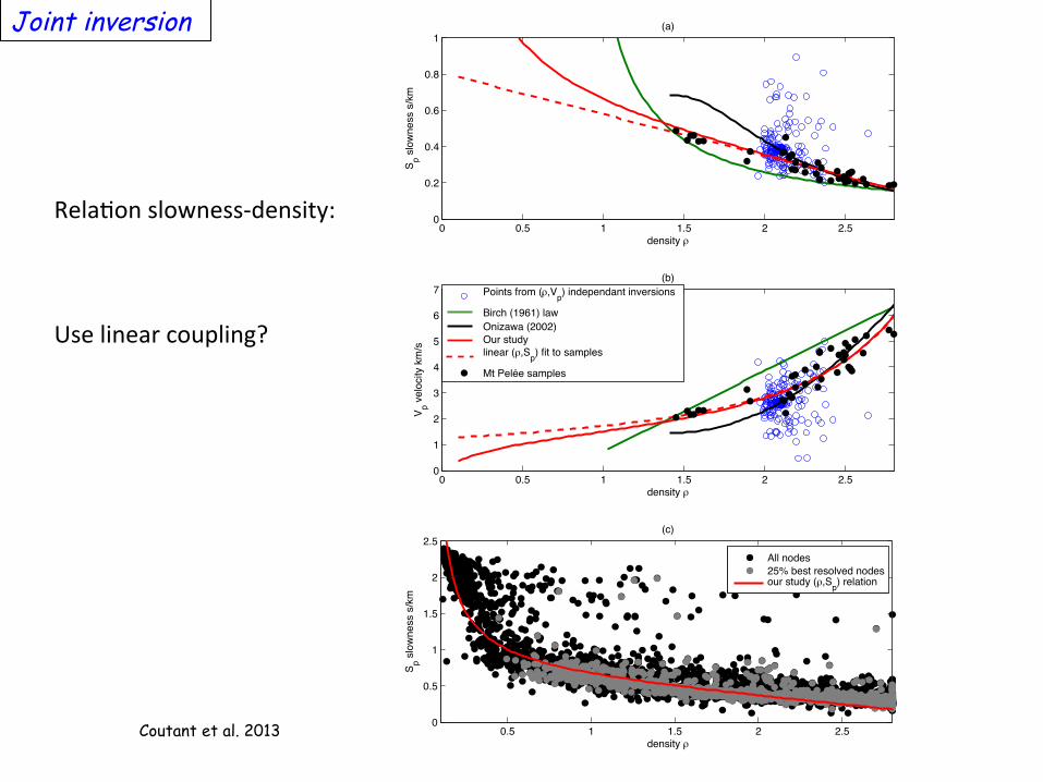
Points from (l,Vp) independant inversions

Birch (1961) law

Onizawa (2002)

Our study

linear (l,Sp) fit to samples

Mt Pelée samples

0.5 1 1.5 2 2.50

0.5

1

1.5

2

2.5

25% best resolved nodes

our study (l,Sp) relation

density l

Sp s

low

ness s

/km

(c)

All nodes

25% best resolved nodes

our study (l,Sp) relation

Rela%on slowness-‐density: Use linear coupling?

Coutant et al. 2013

Joint inversion: an experiment

A joint inversion: seismic and gravity on a volcano (active…)

Two dykes

Horizontal travel time

Seismic and gravimetric stations

(ρ, S)

ρ=2700 Vp=2000

Ttime = SiXinodes∑

Gravity = ρiGinodes∑

A joint inversion: seismic and gravity on a volcano (active…)

Two dykes

Horizontal travel time

Seismic and gravimetric stations

(ρ, S)


ρ=2700 Vp=2000

Ttime = SiXinodes∑

Gravity = ρiGinodes∑

How to solve ? Assume a linear coupling between ρ and S:

G .m−d Cd

2+ m−mprior Cm

2+ S− f (ρ ) Cρ

2

data model coupling


G .m−d Cd

2+ m−mprior Cm

2

m =

np × slowness dyke1np × slowness dyke 2np × density dyke1np × density dyke 2

⎡

⎣

⎢⎢⎢⎢⎢

⎤

⎦

⎥⎥⎥⎥⎥

d =ns× travel times

ns× gravity left slopens× gravity right slope

⎡

⎣

⎢⎢⎢

⎤

⎦

⎥⎥⎥

G =

dTravelTime

dSlowness0

0 dGravity

dρensity

⎡

⎣

⎢⎢⎢⎢⎢

⎤

⎦

⎥⎥⎥⎥⎥

d =G m


Cd =σ t 0 00 σ g 0

0 0 σ g

⎡

⎣

⎢⎢⎢⎢

⎤

⎦

⎥⎥⎥⎥

Cm =

σ Sdyke10 coupling 0

0 σ Sdyke20 0

coupling 0 σ ρdyke1coupling

0 coupling 0 σ ρdyke2

⎡

⎣

⎢⎢⎢⎢⎢⎢

⎤

⎦

⎥⎥⎥⎥⎥⎥

m̂ = mprior + (GTCd

-1G +Cm-1 )-1GTCd

-1 d −G.mprior( )


Independent inversion, no coupling

Joint inversion: parameters


Joint inversion: data fitting


)p://ist-‐)p.ujf-‐grenoble.fr/users/coutanto/JIG.zip

bayesian inversion - joint inversions in geophysics · bayesian inversion • main credits: –...

Documents