bayesian inference for contact networks given epidemic …davidw/davidw_files/groendyke 2011... ·...

Scandinavian Journal of Statisticsdoi: 10.1111/j.1467-9469.2010.00721.x! 2010 Board of the Foundation of the Scandinavian Journal of Statistics. Published by Blackwell Publishing Ltd.

Bayesian Inference for Contact NetworksGiven Epidemic DataCHRIS GROENDYKEDepartment of Statistics, Pennsylvania State University

DAVID WELCH and DAVID R. HUNTERDepartment of Statistics and Center for Infectious Disease Dynamics, PennsylvaniaState University

ABSTRACT. In this article, we estimate the parameters of a simple random network and a stochas-tic epidemic on that network using data consisting of recovery times of infected hosts. The SEIRepidemic model we fit has exponentially distributed transmission times with Gamma distributedexposed and infectious periods on a network where every edge exists with the same probability,independent of other edges. We employ a Bayesian framework and Markov chain Monte Carlo(MCMC) integration to make estimates of the joint posterior distribution of the model parameters.We discuss the accuracy of the parameter estimates under various prior assumptions and show thatit is possible in many scientifically interesting cases to accurately recover the parameters. We dem-onstrate our approach by studying a measles outbreak in Hagelloch, Germany, in 1861 consistingof 188 affected individuals. We provide an R package to carry out these analyses, which is availablepublicly on the Comprehensive R Archive Network.

Key words: Erdos-Renyi, exponential random graph model (ERGM), MCMC, measles,stochastic SEIR epidemic

1. Introduction

In studying the dynamics of epidemics, the dominant model has long been the ‘mean field’or ‘random mixing’ model that assumes that an infectious individual may spread thedisease to any susceptible member of the population (Kermack & McKendrick, 1927; Bailey,1950). An alternate assumption under which the epidemic spreads only across the edgesof a contact network within a population may result in much different epidemic dynamics(Keeling & Eames, 2005; Meyers et al., 2005; Ferrari, 2006). Much of the work based onthis alternate assumption relies heavily on simulations. Some network is taken as given orsimulated to have certain properties, then a disease outbreak is simulated on the networkand the properties of the epidemic studied; see, for example, Volz (2008) and Barthelemyet al. (2005).

This article takes a different approach, extending work of Britton & O’Neill (2002) to con-sider the central question of statistical inference: Given epidemic data assumed to have arisenfrom the spread of some disease across a network, what can we say about the properties ofthe disease spread and the network on which it spread? Ascertaining these properties willallow us to learn about the contact networks associated with certain diseases, thereby enablingresearchers to test competing theories about transmission of disease and to devise bettercontainment strategies. In particular, we address some of the practical issues of implementingthe framework described by Britton & O’Neill (2002) such as determining the areas of theparameter space in which parameter estimation might be expected to be fruitful andimplementing the software necessary to perform the type of inference described; we also suggestgeneralizations of the network model used in Britton & O’Neill (2002). The primary purpose

2 C. Groendyke et al. Scand J Statist

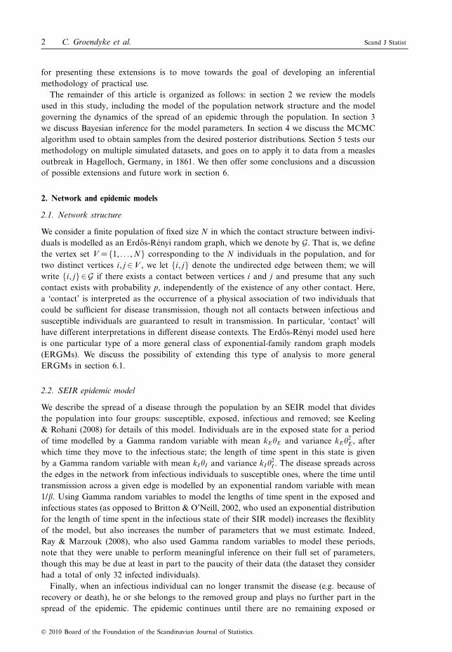
for presenting these extensions is to move towards the goal of developing an inferentialmethodology of practical use.

The remainder of this article is organized as follows: in section 2 we review the modelsused in this study, including the model of the population network structure and the modelgoverning the dynamics of the spread of an epidemic through the population. In section 3we discuss Bayesian inference for the model parameters. In section 4 we discuss the MCMCalgorithm used to obtain samples from the desired posterior distributions. Section 5 tests ourmethodology on multiple simulated datasets, and goes on to apply it to data from a measlesoutbreak in Hagelloch, Germany, in 1861. We then offer some conclusions and a discussionof possible extensions and future work in section 6.

2. Network and epidemic models

2.1. Network structure

We consider a finite population of fixed size N in which the contact structure between indivi-duals is modelled as an Erdos-Rényi random graph, which we denote by G. That is, we definethe vertex set V ={1, . . ., N} corresponding to the N individuals in the population, and fortwo distinct vertices i, j ! V , we let {i, j} denote the undirected edge between them; we willwrite {i, j}!G if there exists a contact between vertices i and j and presume that any suchcontact exists with probability p, independently of the existence of any other contact. Here,a ‘contact’ is interpreted as the occurrence of a physical association of two individuals thatcould be sufficient for disease transmission, though not all contacts between infectious andsusceptible individuals are guaranteed to result in transmission. In particular, ‘contact’ willhave different interpretations in different disease contexts. The Erdos-Rényi model used hereis one particular type of a more general class of exponential-family random graph models(ERGMs). We discuss the possibility of extending this type of analysis to more generalERGMs in section 6.1.

2.2. SEIR epidemic model

We describe the spread of a disease through the population by an SEIR model that dividesthe population into four groups: susceptible, exposed, infectious and removed; see Keeling& Rohani (2008) for details of this model. Individuals are in the exposed state for a periodof time modelled by a Gamma random variable with mean kE!E and variance kE!2

E , afterwhich time they move to the infectious state; the length of time spent in this state is givenby a Gamma random variable with mean kI !I and variance kI !

2I . The disease spreads across

the edges in the network from infectious individuals to susceptible ones, where the time untiltransmission across a given edge is modelled by an exponential random variable with mean1/". Using Gamma random variables to model the lengths of time spent in the exposed andinfectious states (as opposed to Britton & O’Neill, 2002, who used an exponential distributionfor the length of time spent in the infectious state of their SIR model) increases the flexiblityof the model, but also increases the number of parameters that we must estimate. Indeed,Ray & Marzouk (2008), who also used Gamma random variables to model these periods,note that they were unable to perform meaningful inference on their full set of parameters,though this may be due at least in part to the paucity of their data (the dataset they considerhad a total of only 32 infected individuals).

Finally, when an infectious individual can no longer transmit the disease (e.g. because ofrecovery or death), he or she belongs to the removed group and plays no further part in thespread of the epidemic. The epidemic continues until there are no remaining exposed or

! 2010 Board of the Foundation of the Scandinavian Journal of Statistics.

Scand J Statist Network inference using epidemic data 3

infectious individuals in the population. Clearly, the dynamics of the epidemic and theproportion of the population that becomes infected depend heavily on the parameters in thenetwork model (p) and in the epidemic model (", kE , !E , kI , !I ). While we are not aware ofany statistical or probabilistic analyses of this model in the literature, there have been severalstudies that simulate SEIR outbreaks on Erdos-Rényi networks (Rahmandad & Sterman,2008; Kenah, 2009).

3. Inference

3.1. Data and notation

The data we consider are the removal times for each infected node. The data may also includethe exposure and/or infectious times for each node, but in general, these will be unknown.The exposure, infectious and removal times for node j are denoted by Ej , Ij and Rj , respec-tively. The sets of all exposure, infectious and removal times are E = (E1, E2, . . ., EN ),I = (I1, I2, . . ., IN ), and R = (R1, R2, . . ., RN ); we will denote the entire set of times (E, I, R) byT. We assign a value of " to Eb, Ib and Rb for any node b that was not infected during thecourse of the epidemic. Denote the identity of the initial exposed by #; since the identity ofthis individual will not in general be known, # may be considered a parameter to estimate.Because we will sometimes need to treat the exposure time of the initial exposed separatelyfrom that of the other infecteds, we denote by E## the set of the exposure times except forthe initial exposed, that is, E\E#. For convenience, we label the nodes so that the ones whowere infected during the epidemic are 1, . . ., m, where m is the number of nodes that wereultimately infected, and 1$m$N .

For this analysis, we perform inference on the model parameters using a Bayesianapproach. We will denote the prior distribution for a generic parameter (say, $) by %$(·),the likelihood function by L(T |$, . . .), and the posterior distribution of $ by %$(· |T).

Denote the fixed but unknown contact network in the population by G and the associatedtransmission tree (pathway along which the epidemic spreads) by P . P , whose root node is#, is a directed subgraph of the undirected graph G. We will say that the edge (a, b)!P iff ainfects b. Note that if (a, b)!P , we must have

Ia < Eb < Ra. (1)

We also have the following relationships: m # 1= |P|$|G|$!N

2

", where |P| and |G| denote

the number of (directed) edges in P and the number of (undirected) edges in G, respectively.This notation borrows from and extends that used in Britton & O’Neill (2002).

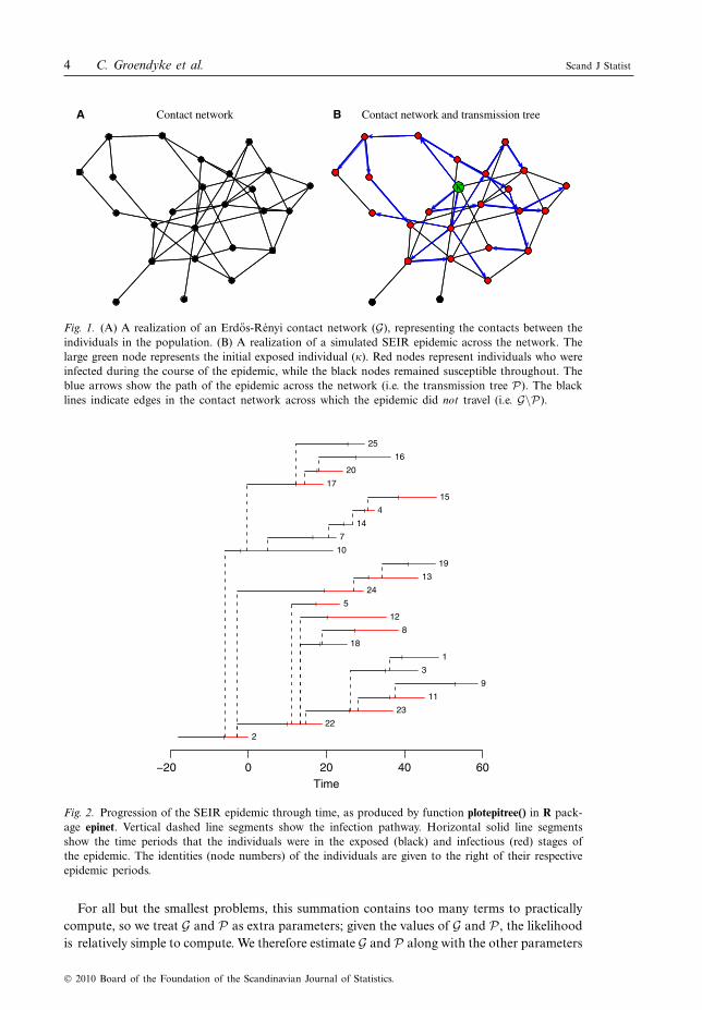
Figure 1A shows an example of a contact network G within a population of N =25 indivi-duals. This network was simulated using an Erdos-Rényi model with p=0.15. Superimposedon this contact network in Fig. 1B is the transmission tree P generated from a simulatedSEIR stochastic epidemic, with "=0.15 and kI =kE =!I =!E =3. Figure 2 illustrates thespread of this epidemic over time.

3.2. Likelihood calculation

To calculate the likelihood function for this model, it would be necessary to sum over allpossible values of G and P :

L(T |", kE , !E , kI , !I , p)=#

G,P

L(T |", kE , !E , kI , !I , p, G, P) f (G, P |p)

=#

G

#

P

L(T |", kE , !E , kI , !I , p, G, P) f (P |G) f (G |p).



"

A Contact network Contact network and transmission treeB

Fig. 1. (A) A realization of an Erdos-Renyi contact network (G), representing the contacts between theindividuals in the population. (B) A realization of a simulated SEIR epidemic across the network. Thelarge green node represents the initial exposed individual (#). Red nodes represent individuals who wereinfected during the course of the epidemic, while the black nodes remained susceptible throughout. Theblue arrows show the path of the epidemic across the network (i.e. the transmission tree P). The blacklines indicate edges in the contact network across which the epidemic did not travel (i.e. G\P).

!20 0 20 40 60Time

2

10

24

22

17

7

5

25

12

18

20

23

16

8

14

3

4

13

11

15

19

1

9

l

l

l

l

l

l

l

l

l

l

l

l

l

l

l

l

l

l

l

l

l

l

l

Fig. 2. Progression of the SEIR epidemic through time, as produced by function plotepitree() in R pack-age epinet. Vertical dashed line segments show the infection pathway. Horizontal solid line segmentsshow the time periods that the individuals were in the exposed (black) and infectious (red) stages ofthe epidemic. The identities (node numbers) of the individuals are given to the right of their respectiveepidemic periods.

For all but the smallest problems, this summation contains too many terms to practicallycompute, so we treat G and P as extra parameters; given the values of G and P , the likelihoodis relatively simple to compute. We therefore estimate G and P along with the other parameters



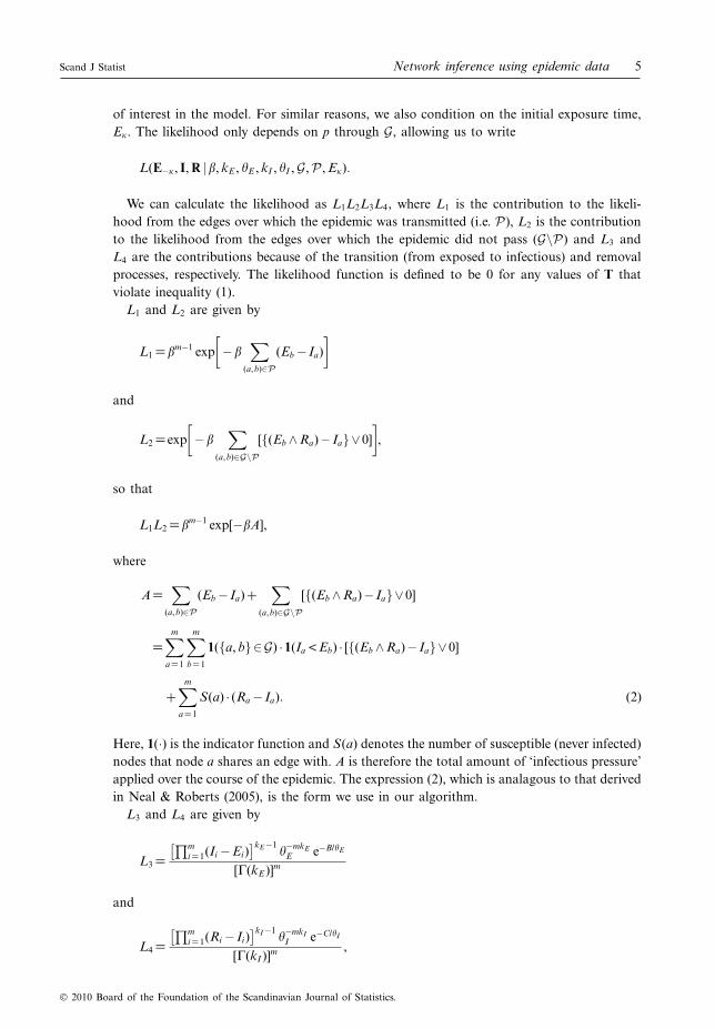
of interest in the model. For similar reasons, we also condition on the initial exposure time,E#. The likelihood only depends on p through G, allowing us to write

L(E##, I, R |", kE , !E , kI , !I , G, P , E#).

We can calculate the likelihood as L1L2L3L4, where L1 is the contribution to the likeli-hood from the edges over which the epidemic was transmitted (i.e. P), L2 is the contributionto the likelihood from the edges over which the epidemic did not pass (G\P) and L3 andL4 are the contributions because of the transition (from exposed to infectious) and removalprocesses, respectively. The likelihood function is defined to be 0 for any values of T thatviolate inequality (1).

L1 and L2 are given by

L1 ="m#1 exp$

#"#

(a,b)!P

(Eb # Ia)%

and

L2 = exp$

#"#

(a,b)!G\P

[{(Eb %Ra)# Ia}&0]%,

so that

L1L2 ="m#1 exp[#"A],

where

A=#

(a,b)!P

(Eb # Ia)+#

(a,b)!G\P

[{(Eb %Ra)# Ia}&0]

=m#

a =1

m#

b=1

1({a, b}!G) ·1(Ia < Eb) · [{(Eb %Ra)# Ia}&0]

+m#

a =1

S(a) · (Ra # Ia). (2)

Here, 1(·) is the indicator function and S(a) denotes the number of susceptible (never infected)nodes that node a shares an edge with. A is therefore the total amount of ‘infectious pressure’applied over the course of the epidemic. The expression (2), which is analagous to that derivedin Neal & Roberts (2005), is the form we use in our algorithm.

L3 and L4 are given by

L3 =&'m

i =1(Ii #Ei)(kE #1

!#mkEE e#B/!E

[!(kE )]m

and

L4 =&'m

i =1(Ri # Ii)(kI #1

!#mkII e#C/!I

[!(kI )]m ,



where B =)mi =1(Ii # Ei) and C =)m

i =1(Ri # Ii) are the total amounts of time spent by allindividuals in the exposed and infectious states, respectively.

3.3. Prior distributions

For some model parameters, we typically use conjugate prior distributions; these distributionsare often preferable when they are available, as they can simplify and/or accelerate the processof updating these parameters. In particular, the beta distribution is conjugate for the networkparameter p; the inverse Gamma distribution is conjugate for the epidemic parameters !E

and !I ; and the Gamma distribution is conjugate for the parameter ". When it is necessaryto infer the exposure and/or infectious times, we assign them uninformative (flat) prior distri-butions; when necessary, we assign a prior for # that is uniform on 1, . . ., m. For the kE andkI parameters, we use Gamma or uniform prior distributions.

In choosing parameters for the prior distributions, we can obtain guidance from indepen-dent information known about the disease and/or population, as well as from the scientificliterature in some cases. For example, much work has been performed to study the lengthsof times that individuals infected with the measles virus spend in the exposed and infectiousstates; we can use this information to constuct prior distributions for the parameters govern-ing these periods. Regarding the parameter p, if we have reason to believe that the networkunder consideration is likely to be sparse, we might then choose a beta distribution that placesgreater mass on the smaller values of p.

4. MCMC algorithm

Here, we describe the MCMC algorithm used to produce samples from the posterior distri-butions of the parameters. At each iteration, we update each parameter in turn: {P , G, p,", kE , !E , kI , !I , I, E, #}, using the methods described next. Experimentation indicates thatupdating the parameters in a fixed order results in better mixing of the Markov chain thanchoosing a random update order for each cycle. Note that in the case where the exposuretimes are assumed to be known, we do not update E; similarly, when the infectious timesare known, we need not update I. Only in the case in which both E and I are unknown dowe need to infer #. This algorithm is based in part on the algorithm described in Britton &O’Neill (2002). However, we did not find that the ‘mixing step’ described by those authorssignificantly improved the performance of the algorithm, and hence did not include it in ouralgorithm. Neal & Roberts (2005) give an algorithm based on a different representation ofthe network model; we discuss the relative merits of the two parameterizations in section 4.6.

4.1. Updating kE , kI , p, ", !E , !I

These parameters can be updated via a standard Hastings step. We propose updated val-ues from a uniform distribution centred at the current value of the parameter. Alternatively,the p, ", !E and !I parameters can be updated using Gibbs samplers from their conditionaldistributions, if appropriate prior distributions are used. Let X 'Gamma(a, b) indicate that Xhas a Gamma distribution with density xa#1b#a e#x/b/!(a) for x > 0; let W ' IG(c, d) indicatethat W has an inverse Gamma distribution, that is, 1/W 'Gamma(c, 1/d); let Y 'beta(q, z)indicate that Y has a beta distribution with parameters q and z on (0, 1); and let U 'U(a, b)indicate that U has a uniform distribution on (a, b).

If we assign the following prior distributions as described in section 3.3: %"(") 'Gamma(a", b"), %!I (!I ) ' IG(aI , bI ), %!E (!E ) ' IG(aE , bE ) and %p(p) ' beta(c, d), then thecorresponding full conditional distributions of these parameters are:



%"(" |T)'Gamma*

m+a" #1,1

A+1/b"

+,

%!E (!E |T)' IG*

mkE +aE ,1

B +1/bE

+,

%!I (!I |T)' IG*

mkI +aI ,1

C +1/bI

+and

%p(p |T)'beta*

|G|+ c,*

N2

+# |G|+d

+,

where A, B and C are as defined in section 3.2.

4.2. Updating G

Since we are assuming that the existence of each edge is independent of all other edges, wecan generate each edge individually to sample from the full conditional distribution of G.We calculate the full conditional probability of the event {i, j}!G, which we denote by Dij ,assuming without loss of generality that Ei < Ej :

P(Dij |T, P , ", p)= P(T |Dij , P , ", p)P(Dij |P , ", p)P(T |Dij , P , ", p)P(Dij |P , ", p)+P(T |Dc

ij , P , ", p)P(Dcij |P , ", p)

,

where P(Dij |P , ", p)=p, unless the edge (i, j) is in P , in which case P(Dij |P , ", p)=1. Thevalues of P(T |Dij , P , ", p) and P(T |Dc

ij , P , ", p) vary depending on the status (ultimatelyinfected or never infected) of nodes i and j. Note that we only need to consider the data asso-ciated with these two nodes, rather than the entirety of T. If (i, j) !P then P(Dij |T, P , ", p)=1,since (i, j)!P ({i, j}!G. Otherwise, if (i, j) )!P , then

P(Dij |T, P , ", p)= exp(#"[{(Ri %Ej)# Ii}&0]) ·p1#p+ exp(#"[{(Ri %Ej)# Ii}&0]) ·p

.

Recall that Ek = Ik =Rk =" for k > m; we also use the convention that " # "=0 for thepurpose of evaluating the aforesaid probabilities.

4.3. Updating P

Updating the transmission tree consists of determining, for each infected node except theinitial exposed, which node infected it. Let Pj denote the parent of node j and %Pj (r) denotethe prior probability that node r is the parent of j. The candidate nodes for the parent of nodej (i.e. the node that infected j) are exactly those nodes i for which {i, j}!G and Ii $Ej $Ri .

Denote these candidate nodes by i1, . . ., ik . Then the probability that it is the parent of j,given that one of the candidates is known to have infected j, is

" exp(#")

i!{i1, ..., ik}[Ej # Ii ]) ·%Pj (it))k

a =1" exp(#")

i!{i1, ..., ik}[Ej # Ii ]) ·%Pj (ia)=

%Pj (it))k

a =1%Pj (ia)

a function of only the prior assumptions. If we assume that %Pj (r) is the same for all j and r(we will often make this uniform assumption in the absence of other information, though weconsider other possibilities in section 5.2.2), then each of the candidates is equally likely tobe the parent. To find the parent of node j, we simply find the parent candidates and sample



from among them according to their respective probabilities. We repeat this for each infectednode (except the initial exposed) to produce a sample from the full conditional distributionof P .

4.4. Updating #

Note that we only need to update # in the cases in which both E and I are not fully known.To perform this update, we use a method similar to that described by Britton & O’Neill(2002). The typical prior assumption is that each of the m infected nodes is equally likely tobe the initial infected, that is, %#(i)=1/m for all i. Given the current value of #, we choosea proposed value for #* by sampling uniformly from the set {j : (#, j)!P}. We propose newvalues for P , E and I that are consistent with #* in the following manner. First, we swap thevalues of E# and I# with those of E#* and I#* , respectively. Then, we replace the edge (#, #*)in P with (#*, #). We determine whether or not to accept the proposed values according tothe appropriate Hastings ratio.

4.5. Updating E, I

We update each element of E## in a uniformly random order, and finally update E#. We use aHastings step to update each element of E. For each j /=#, we first identify the parent of j inP , that is, the node that infected j. Since i must have been infectious (and not yet recovered)when j became exposed, and since j enters the exposed phase before the infectious phase,we must have Ii < Ej < min{Ij , Ri}. The proposed updated value for Ej is generated from auniform distribution on the interval of its possible values.

Our method for updating I is similar to that for E, updating each Ij in a uniformly randomorder. We find a proposed value for each Ij by sampling uniformly from the interval of itspossible values and accept each proposal according to the appropriate Hastings ratio.

4.6. Implementation

We have built a package for R (R Development Core Team, 2010), named epinet, containingsoftware which implements the algorithm described before. This software is publicly availableon the Comprehensive R Archive Network (CRAN; cran.r-project.org), and will in the futurebe maintained to reflect future extensions and/or generalizations made to the model, such asthe ERGM extensions discussed in section 6.1.

The internal representation of the graph structure, which is based on the binary treerepresentation used in the ergm package (Handcock et al., 2010), allows for efficientstorage of the graph, especially for sparse graphs. There are several reasons that we chose toextend the MCMC algorithm described in Britton & O’Neill (2002), rather than the algorithmdetailed in Neal & Roberts (2005). The first reason is scalability. As noted by Neal & Roberts(2005), it is not necessary to know the entirety of the graph G to calculate the likelihood forour model. Neal & Roberts (2005) propose using a subgraph F that does not consider theedges between never-infected individuals; this subgraph consists of N · m dyads. Our algo-rithm, using the expression for the likelihood given in (2), only explicitly considers the edgesbetween two infected individuals. We also must keep track of the number of never-infectedindividuals that each of the m infecteds is connected to. Thus, the algorithm we describerequires storage and updating of m2 +m rather than N ·m elements. In cases where N +m,that is, when only a small portion of a population is infected, this savings in computingresources may be significant.



In our experience, the algorithm described by Neal & Roberts (2005) ran significantly moreslowly than did the algorithm described in section 4. When the parameter p is updated in theNeal and Roberts algorithm, each edge in F is also updated, causing this update to be veryslow. This situation will only worsen as we move to more complicated ERGM models (seesection 6.1) which have more parameters, as F would need to be updated with each of them.The two methods gave roughly similar results in terms of mixing, as measured by numberof effective samples produced, though the relative performances of the algorithms varied byparameter and dataset.

5. Applications

5.1. Simulated epidemics

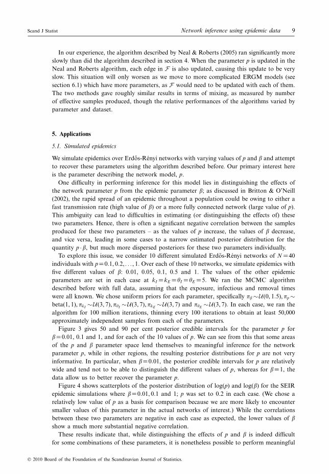
We simulate epidemics over Erdos-Rényi networks with varying values of p and " and attemptto recover these parameters using the algorithm described before. Our primary interest hereis the parameter describing the network model, p.

One difficulty in performing inference for this model lies in distinguishing the effects ofthe network parameter p from the epidemic parameter "; as discussed in Britton & O’Neill(2002), the rapid spread of an epidemic throughout a population could be owing to either afast transmission rate (high value of ") or a more fully connected network (large value of p).This ambiguity can lead to difficulties in estimating (or distinguishing the effects of) thesetwo parameters. Hence, there is often a significant negative correlation between the samplesproduced for these two parameters – as the values of p increase, the values of " decrease,and vice versa, leading in some cases to a narrow estimated posterior distribution for thequantity p ·", but much more dispersed posteriors for these two parameters individually.

To explore this issue, we consider 10 different simulated Erdos-Rényi networks of N =40individuals with p=0.1, 0.2, . . ., 1. Over each of these 10 networks, we simulate epidemics withfive different values of ": 0.01, 0.05, 0.1, 0.5 and 1. The values of the other epidemicparameters are set in each case at kI =kE =!I =!E =5. We ran the MCMC algorithmdescribed before with full data, assuming that the exposure, infectious and removal timeswere all known. We chose uniform priors for each parameter, specifically %" 'U(0, 1.5), %p 'beta(1, 1), %kI 'U (3, 7), %!I 'U (3, 7), %kE 'U (3, 7) and %!E 'U(3, 7). In each case, we ran thealgorithm for 100 million iterations, thinning every 100 iterations to obtain at least 50,000approximately independent samples from each of the parameters.

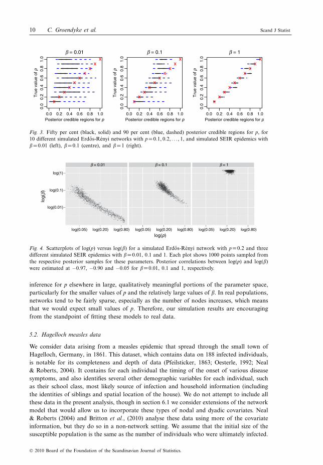
Figure 3 gives 50 and 90 per cent posterior credible intervals for the parameter p for"=0.01, 0.1 and 1, and for each of the 10 values of p. We can see from this that some areasof the p and " parameter space lend themselves to meaningful inference for the networkparameter p, while in other regions, the resulting posterior distributions for p are not veryinformative. In particular, when "=0.01, the posterior credible intervals for p are relativelywide and tend not to be able to distinguish the different values of p, whereas for "=1, thedata allow us to better recover the parameter p.

Figure 4 shows scatterplots of the posterior distribution of log(p) and log(") for the SEIRepidemic simulations where "=0.01, 0.1 and 1; p was set to 0.2 in each case. (We chose arelatively low value of p as a basis for comparison because we are more likely to encountersmaller values of this parameter in the actual networks of interest.) While the correlationsbetween these two parameters are negative in each case as expected, the lower values of "show a much more substantial negative correlation.

These results indicate that, while distinguishing the effects of p and " is indeed difficultfor some combinations of these parameters, it is nonetheless possible to perform meaningful



0.0 0.2 0.4 0.6 0.8 1.0

0.0

0.2

0.4

0.6

0.8

1.0

b = 0.01

Posterior credible regions for p Posterior credible regions for p Posterior credible regions for p

Tru

e va

lue

of p

Tru

e va

lue

of p

Tru

e va

lue

of p

xx

xx

xx

xx

xx

0.0 0.2 0.4 0.6 0.8 1.0

0.0

0.2

0.4

0.6

0.8

1.0

b = 0.1

xx

xx

xx

xx

xx

0.0 0.2 0.4 0.6 0.8 1.0

0.0

0.2

0.4

0.6

0.8

1.0

b = 1

xx

xx

xx

xx

xx

Fig. 3. Fifty per cent (black, solid) and 90 per cent (blue, dashed) posterior credible regions for p, for10 different simulated Erdos-Renyi networks with p=0.1, 0.2, . . ., 1, and simulated SEIR epidemics with"=0.01 (left), "=0.1 (centre), and "=1 (right).

log(p)

log(

b)

log(0.01)

log(0.1)

log(1)

b = 0.01

log(0.05) log(0.20) log(0.80) log(0.05) log(0.20) log(0.80) log(0.05) log(0.20) log(0.80)

b = 0.1 b = 1

Fig. 4. Scatterplots of log(p) versus log(") for a simulated Erdos-Renyi network with p=0.2 and threedifferent simulated SEIR epidemics with "=0.01, 0.1 and 1. Each plot shows 1000 points sampled fromthe respective posterior samples for these parameters. Posterior correlations between log(p) and log(")were estimated at #0.97, #0.90 and #0.05 for "=0.01, 0.1 and 1, respectively.

inference for p elsewhere in large, qualitatively meaningful portions of the parameter space,particularly for the smaller values of p and the relatively large values of ". In real populations,networks tend to be fairly sparse, especially as the number of nodes increases, which meansthat we would expect small values of p. Therefore, our simulation results are encouragingfrom the standpoint of fitting these models to real data.

5.2. Hagelloch measles data

We consider data arising from a measles epidemic that spread through the small town ofHagelloch, Germany, in 1861. This dataset, which contains data on 188 infected individuals,is notable for its completeness and depth of data (Pfeilsticker, 1863; Oesterle, 1992; Neal& Roberts, 2004). It contains for each individual the timing of the onset of various diseasesymptoms, and also identifies several other demographic variables for each individual, suchas their school class, most likely source of infection and household information (includingthe identities of siblings and spatial location of the house). We do not attempt to include allthese data in the present analysis, though in section 6.1 we consider extensions of the networkmodel that would allow us to incorporate these types of nodal and dyadic covariates. Neal& Roberts (2004) and Britton et al., (2010) analyse these data using more of the covariateinformation, but they do so in a non-network setting. We assume that the initial size of thesusceptible population is the same as the number of individuals who were ultimately infected.



This is based on the fact that all of the infected were children born after the previous out-break in Hagelloch and nearly all such children were infected. Detailed justification of thisassumption is given in Neal & Roberts (2004). We assume that each individual’s infectiousperiod begins 1 day prior to the onset of prodromes and ends 3 days after the appearance ofrash (or at death, if sooner). As the data do not contain any information about the exposuretimes of the individuals (E), we will treat these times as unknown and infer them.

We initially performed inference on this dataset under two different sets of prior assumptionsfor the parameters. In the first case, we used uniform priors for all parameters, so %" 'U(0, 2),%p ' U (0, 1), %kI ' U (15, 25), %!I ' U (0.25, 0.75), %kE ' U(8, 20) and %!E ' U(0.25, 1). In thesecond case, we used the conjugate prior distributions described in section 4.1, so that %" 'Gamma(2, 0.5), %p ' beta(1, 1), %kI ' Gamma(20, 1), %!I ' IG(3.5, 1), %kE ' Gamma(20, 1) and%!E ' IG(3.5, 1). In both cases, we used uniform priors for the transmission tree. There is oneindividual in the dataset who is recorded as showing symptoms of the disease approximately1 month after the epidemic had otherwise subsided, making inclusion of this individual inthe epidemic questionable. We ran our analyses both including and excluding this individual.In each case, we ran the algorithm for 20 million iterations, thinning every 200 iterations toobtain at least 5000 approximately independent samples from each of the parameters.

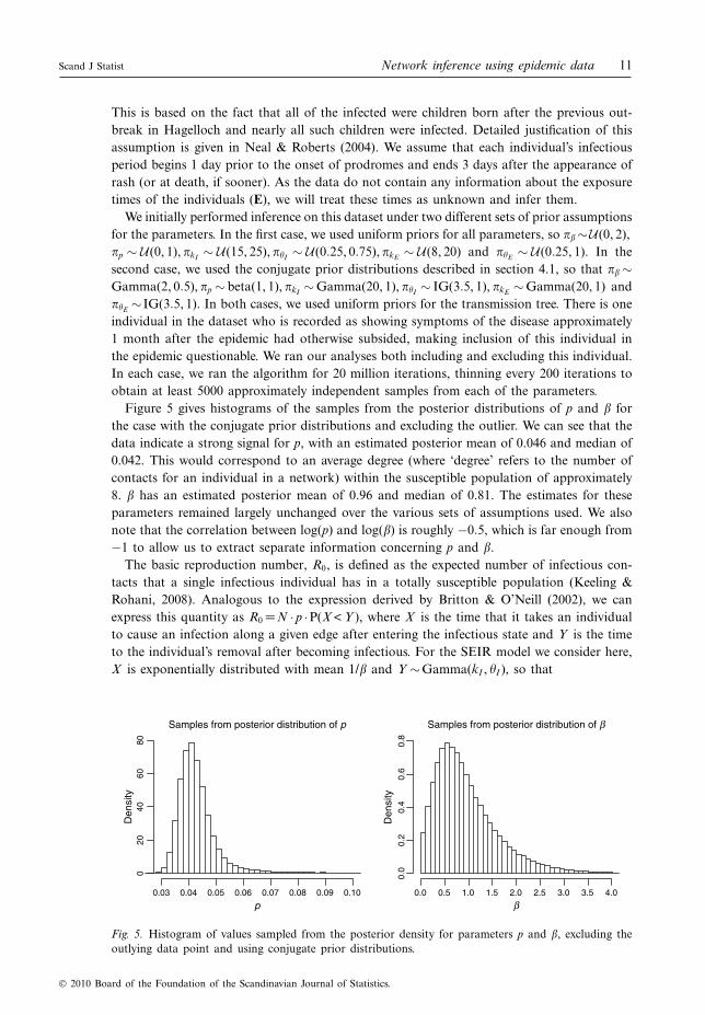
Figure 5 gives histograms of the samples from the posterior distributions of p and " forthe case with the conjugate prior distributions and excluding the outlier. We can see that thedata indicate a strong signal for p, with an estimated posterior mean of 0.046 and median of0.042. This would correspond to an average degree (where ‘degree’ refers to the number ofcontacts for an individual in a network) within the susceptible population of approximately8. " has an estimated posterior mean of 0.96 and median of 0.81. The estimates for theseparameters remained largely unchanged over the various sets of assumptions used. We alsonote that the correlation between log(p) and log(") is roughly #0.5, which is far enough from#1 to allow us to extract separate information concerning p and ".

The basic reproduction number, R0, is defined as the expected number of infectious con-tacts that a single infectious individual has in a totally susceptible population (Keeling &Rohani, 2008). Analogous to the expression derived by Britton & O’Neill (2002), we canexpress this quantity as R0 =N ·p ·P(X < Y ), where X is the time that it takes an individualto cause an infection along a given edge after entering the infectious state and Y is the timeto the individual’s removal after becoming infectious. For the SEIR model we consider here,X is exponentially distributed with mean 1/" and Y 'Gamma(kI , !I ), so that

Samples from posterior distribution of p

p

Den

sity

0.03 0.04 0.05 0.06 0.07 0.08 0.09 0.10

020

4060

80

Samples from posterior distribution of b

Den

sity

0.0 0.5 1.0 1.5 2.0b

2.5 3.0 3.5 4.0

0.0

0.2

0.4

0.6

0.8

Fig. 5. Histogram of values sampled from the posterior density for parameters p and ", excluding theoutlying data point and using conjugate prior distributions.



R0 =N ·p ·,

1#*

11+"!I

+kI-

. (3)

Note that this expression reduces to the formula given by Britton & O’Neill (2002) in the casethat the length of the infectious periods are modelled by an exponential random variable,that is, kI =1. For the values of the ", !I and kI that we consider in this example, (3) willtypically be slightly less than N ·p, an individual’s mean number of contacts.

Figure 6 gives a histogram of the posterior samples for R0, as calculated by (3) using theposterior parameter samples for ", !I and kI produced by the Hagelloch data analysis. Theposterior mean and median are 7.7 and 7.6, respectively, and a 95 per cent posterior credibleinterval for R0 is (6.4, 9.2). This is comparable with figures reported in the literature onmeasles. For instance, Huang (2008) gives a range of 5.8–14.3; and Edmunds et al. (2001)give a range of 6.1–10.2 for different outbreaks, using data that while much later than theHagelloch data are still from prevaccination Europe. We caution that our results should notbe extrapolated to measles outbreaks in general, since they come from only a single outbreak,but nonetheless our R0 values are consistent with existing results.

The two sets of priors did not result in dramatically different posterior distributions for anyof the parameters (note that the prior assumption for p was actually the same in both cases).We did, however, notice a 10–20 per cent decrease in runtimes for the cases where the conju-gate prior distributions were used; this was because of the ability to sample directly from theconditional distributions of many of the parameters rather than relying on computationallyexpensive Metropolis–Hastings steps.

Because we were required to infer the exposure times in this epidemic, it is also interestingto examine the posterior estimates for the parameters governing the exposed periods of theindividuals. As we are using a Gamma(kE , !E ) random variable to model the lengths of theseperiods, their estimated mean and variance are given by kE!E and kE!2

E , respectively. Figure 7shows plots of the estimated posterior distributions of these quantities, both including andexcluding the outlying data point.

We can see that removing the outlier from this dataset caused a modest decrease in thethe estimate of the mean exposed period. Much more noticeable, though, is the effect that re-moving this outlier had on the corresponding estimated variance – a decrease of over40 per cent. These results indicate that this outlier was indeed having a large effect on theestimates of the exposed length parameters. None of the other parameters in the model, how-ever, was significantly affected by the inclusion of this outlier. Our posterior mean estimate of10.3 days for the mean length of the exposed period seems quite reasonable; other authors

Posterior samples for R0

R0

Den

sity

5 6 7 8 9 10 11 12

0.0

0.1

0.2

0.3

0.4

0.5

Fig. 6. Posterior samples of the basic reproduction number R0 for the Hagelloch measles data, calculatedusing (3) using conjugate prior distributions and excluding the outlier.



6 8 10 12 14

0.0

0.1

0.2

0.3

0.4

0.5

0.6

Estimated posterior densities for kEqE Estimated posterior densities for kEqE

Den

sity

10.3 (0.7)11.1 (0.8)

1050 15 20

0.00

0.05

0.10

0.15

0.20

0.25

0.30

2

Den

sity

6.7 (1.5)

11.8 (2.7)

Fig. 7. Estimated posterior densities for the mean (kE!E , left panel) and variance (kE!2E , right panel) of

the length of the inferred exposed periods. The solid lines represent estimates based on all data points,while the dashed lines indicate estimates excluding the outlier. The estimated mean (standard deviation)is also given for each density. The prior assumption for kE!E had a mean of 8 and a standard deviationof 6.9; the prior assumption for kE!2

E had a mean of 5.3 and infinite variance.

have estimated the length of this period to be between 6 and 10.3 days for measles (Gough,1977; Anderson & May, 1982; Schenzle, 1984).

Posterior predictive modelling

We assess the quality of fit of the models used for this analysis by simulating SEIR epidemicsover Erdos-Rényi networks, using epidemic and network parameter values sampled from thejoint posterior distribution produced by the Hagelloch data analysis. We then compared thesesimulated epidemics with the original Hagelloch measles epidemic data. One statistic of inter-est is the number of individuals in the infectious stage of the disease, as a function of time.Figure 8 gives a comparison of these epidemic curves for the simulations as compared withthe actual data. We see that the epidemic increases more rapidly, and dies out earlier, thanthe model predicts. However, this is unsurprising given the simplistic contact network model

Day

Num

ber

of in

fect

ives

10

0

20

40

60

80

100

20 30 40 50 60

Fig. 8. Comparison of the number of individuals in the infectious stage of the epidemic, as a functionof time. The individual epidemics simulated from samples taken from the joint posterior distribution ofthe parameters are traced in grey, while the original Hagelloch measles data is plotted in red. Summa-ries (in the form of boxplots) of the number of infectious individuals from across the 1000 simulationsare given at intervals of 5 days.



used here: an Erdos-Rényi model may capture the correct mean degree of a network, but thedegree distribution itself is fully determined once this mean degree is specified. A more realis-tic network model might more accurately capture the tendency for some nodes to have largedegrees, for instance, it should be possible to modify the model to capture effects becauseof household and classroom, as Neal & Roberts (2004) and Britton et al., (2010) identify asimportant factors. Despite the simplicity of the Erdos-Rényi model used here, however, themodel appears to be a useful first approximation to reality.

Incorporating additional information

We next consider a situation in which the data provide additional information beyond theinfectious and removal times considered before. In particular, the Hagelloch dataset containsinformation about the actual transmission tree for this epidemic. For each individual, a ‘puta-tive parent’ is given, that is, the data contain an indication of who is the most likely to haveinfected each individual (Oesterle, 1992). We use this information to construct a more infor-mative prior distribution for the transmission tree P . Rather than assuming a uniform priorfor each node j, that is, %Pj (r) the same for all r, we will incorporate the additional informa-tion by placing more prior weight on the putative parent than on the other individuals.

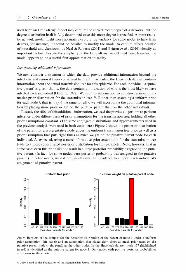
To study the effect of this additional information, we used the previous algorithm to performinference under different sets of prior assumptions for the transmission tree, holding all otherprior assumptions constant. (The same conjugate distributions and hyperparameters used inthe previous analysis were used in both cases here.) Figure 9 shows the posterior distributionof the parent for a representative node under the uniform transmission tree prior as well as aprior assumption that puts eight times as much weight on the putative parent node for eachindividual. As expected, using a more informative prior assumption for the transmission treeleads to a more concentrated posterior distribution for this parameter. Note, however, that insome cases even this prior did not result in a large posterior probability assigned to the puta-tive parent. (In fact, for some nodes, zero posterior probability was assigned to the putativeparent.) In other words, we did not, in all cases, find evidence to support each individual’sassignment of putative parent.

42 45 172 173 174 176 177 179 180 181 182 183

Uniform tree prior

Den

sity

0.0

0.1

0.2

0.3

0.4

0.5

42 45 172 173 174 176 177 180 181 182 183

8 ! Prior weight on putative parent node

Possible parents for node 1Possible parents for node 1

Den

sity

0.0

0.1

0.2

0.3

0.4

0.5

Fig. 9. Barplots of the samples for the posterior distribution of the parent of node 1 under a uniformprior assumption (left panel) and an assumption that places eight times as much prior mass on theputative parent node (right panel) as the other nodes. In the Hagelloch dataset, node 177 (highlightedin red) is identified as the putative parent for node 1. Only nodes with positive posterior probabilitiesare shown in the charts.



We also consider the impact that this additional information will have on the inference forthe others parameters in the model. Incorporating this additional information has almostno impact on the inferential results for the network parameter p, but does have an effecton some of the other parameters. Most notably, increasing the prior weight placed on theputative parent node caused a slight change in the estimated exposure lengths; in particularthe estimated mean exposure length decreased, whereas the estimated variance of the ex-posure periods increased. This is not surprising, given the data. As mentioned before, manyof the assignments of the putative parent node are questionable on the grounds that theywould necessitate unreasonably short exposure periods, some as short as 1 or 2 days. As wegive more prior weight to these assignments, the estimates’ exposure lengths must necessarilydecrease in mean and increase in variance to accomodate.

6. Discussion

Performing inference for the parameters of a network model, given only data about the infec-tious and removal times of individuals, can be very difficult. The examples in the previoussection, however, show that it is indeed possible in many cases to use this type of data toextract meaningful information about the structure of the underlying population. Since thisstructure is known to play an important role in the dynamics of epidemics, developing novelmethods of inferring this structure – a subject which until recently has received relatively littleattention – is potentially very valuable.

In this article, we have extended the framework established by Britton & O’Neill (2002) byusing a more flexible epidemic model and providing efficient computer code to run experi-ments. We ran experiments on simulated datasets to determine which areas of the parameterspace are most likely to provide meaningful results and found that we were able to makegood parameter estimates for a range of biologically plausible values. We have also performedinference for the network and epidemic parameters for an actual dataset under various setsof prior assumptions; the results obtained were shown to be in concordance with the relevantknown scientific information. These developments, demonstrated using efficient new softwarewe have implemented, show that the original framework of Britton & O’Neill (2002) is viablefor datasets much larger than those considered previously in the literature (Britton & O’Neill,2002; Ray & Marzouk, 2008). It suggests that extensions of the model should be explored (seesection 6.1); after all, the Erdos-Rényi network model used here is certainly overly simplistic.In particular, it will be important to consider how to incorporate more data in the networkmodels used. For example, for certain viral diseases we may have genetic data about virusessampled from infected individuals, and because of the relatively rapid rate of mutations thatoccur in the viral genomes, these data can inform the structure of the transmission tree P .We can in turn use this additional information to help improve the quality of the inferencefor the parameters of interest; in fact, for some applications, the samples of the posteriordistributions of P (and perhaps also G) that are produced by the MCMC algorithm maythemselves be of interest. Or we may have information about the physical locations of vari-ous nodes at various times, which could be employed in a more realistic model for the contactnetwork G.

6.1. Extensions of the network model

One of the extensions of the aforegiven model that we might consider consists of using amore general ERGM to model the interactions in population, as opposed to the Erdos-Rényimodel. The ERGM model is very flexible; by specifying various types of graph statistics,



we can achieve a wide variety of possible models, and hence provide a more general frame-work for performing the type of inference described before. This broader class of modelswould allow for the inclusion of additional types of information that might be present in thedata, as is the case for the Hagelloch dataset described in section 5.2, which includes severalindividual- and dyadic-level covariates.

A more complicated ERGM network structure will of course necessitate some modifi-cations to our inference and MCMC algorithm. The likelihood function would need to bemodified to include the entire vector of ERGM parameters (!), rather than just p, so that wewould have

L(E, I, R |", kE , !E , kI , !I , !)=#

G,P

L(E, I, R |", kE , !E , kI , !I , !, G, P) f (G, P |!)

=#

G

#

P

L(E, I, R |", kE , !E , kI , !I , !, G, P) f (P |G) f (G |!).

We will have to modify the MCMC algorithm described in section 4 to reflect the moregeneral ERGM case. For instance, updating the ! parameter via a Metropolis–Hastings algo-rithm would be more difficult, since the Hastings ratio involves the ratio of ERGM normal-izing constants for the current parameter value !(0) and the new proposal !*. While this ratioof normalizing constants is trivially easy to calculate in the simplistic case of the Erdos-Rényimodel, it is computationally intractable for some other ERGMs (Snijders, 2002; Hunter et al.,2008a). Hence, more complicated updating and estimation schemes such as those describedby Snijders (2002) or Hunter et al. (2008b) may be necessary. Nonetheless, certain types ofERGMs, called dyadic independence models (Hunter et al., 2008a), avoid the difficulties ofestimating the ratio of normalizing constants while still incorporating useful statistics, suchas geographic data on the individual nodes.

Acknowledgements

The authors are grateful to Peter Neal for supplying the Hagelloch dataset and to ShwetaBansal for insightful comments on an early draft of the manuscript. The authors also thanktwo anonymous reviewers for their helpful suggestions, which improved the quality of thearticle. This work was supported by a grant from the National Institutes of Health.

References

Anderson, R. & May, R. (1982). Directly transmitted infections diseases: control by vaccination. Science215, 1053–1060.

Bailey, N. (1950). A simple stochastic epidemic. Biometrika 37, 193–202.Barthelemy, M., Barrat, A., Pastor-Satorras, R. & Vespignani, A. (2005). Dynamical patterns of

epidemic outbreaks in complex heterogeneous networks. J. Theor. Biol. 235, 275–288.Britton, T., Kypraios, T. & O’Neill, P. D. (2010). Inference for epidemics with three levels of mixing:

methodology and application to a measles outbreak. Submitted.Britton, T. & O’Neill, P. (2002). Bayesian inference for stochastic epidemics in populations with random

social structure. Scand. J. Statist. 29, 375–390.Edmunds, W., Gay, N., Kretzschmar, M., Pebody, R. & Wachmann, H. (2001). The pre-vaccination

epidemiology of measles mumps and rubella in Europe: implications for modelling studies. Epidemiol.Infect. 125, 635–650.

Ferrari, M. (2006). Mixing models and the geometry of epidemics, PhD thesis. Pennsylvania StateUniversity, PA.

Gough, K. (1977). The estimation of latent and infectious periods. Biometrika 64, 559–565.Handcock, M. S., Hunter, D. R., Butts, C. T., Goodreau, S. M., Morris, M. & Krivitsky, P. (2010). ergm:

a package to fit simulate and diagnose exponential-family models for networks, version 2.2–3. Seattle,WA. Available on http://CRAN.R-project.org/package=ergm (accessed October 28, 2010).



Huang, S. (2008). A new SEIR epidemic model with applications to the theory of eradication and controlof diseases, and to the calculation of R0. Math. Biosci. 215, 84–104.

Hunter, D. R., Goodreau, S. M. & Handcock, M. S. (2008a). Goodness of fit for social network models.J. Amer. Statist. Assoc. 103, 248–258.

Hunter, D. R., Handcock, M. S., Butts, C. T., Goodreau, S. M. & Morris, M. (2008b). ergm: a packageto fit simulate and diagnose exponential-family models for networks. J. Stat. Softw. 24, 1–29.

Keeling, M. & Eames, K. (2005). Networks and epidemic models. J. Roy. Soc. Interface 2, 295–307.Keeling, M. & Rohani, P. (2008). Modeling infectious diseases in humans and animals. Clin. Infect. Dis.

47, 864–866.Kenah, E. (2009). Contact intervals, survival analysis of epidemic data, and estimation of R0. Arxiv

preprint arXiv:0912.3330.Kermack, W. & McKendrick, A. (1927). A contribution to the mathematical theory of epidemics. Proc.

R. Soc. Lond. Ser. A Math. Phys. Eng. Sci. 115, 700–721.Meyers, L., Pourbohloul, B., Newman, M., Skowronski, D. & Brunham, R. (2005). Network theory and

SARS: predicting outbreak diversity. J. Theor. Biol. 232, 71–81.Neal, P. & Roberts, G. (2004). Statistical inference and model selection for the 1861 Hagelloch measles

epidemic. Biostatistics 5, 249–261.Neal, P. & Roberts, G. (2005). A case study in non-centering for data augmentation: stochastic epidemics.

Statist. Comput. 15, 315–327.Oesterle, H. (1992). Statistiche Reanalyse einer Masernepidemiie 1861 in Hagelloch, MD thesis,

Eberhard-Karls Universität, Tübingen.Pfeilsticker, A. (1863). Beiträge zur Pathologie der Masern mit besonderer Berücksichtigung der statistis-

chen Verhältnisse, MD thesis. Eberhard-Karls Universität, Tübingen.R Development Core Team (2010). R: a language and environment for statistical computing. R Foun-

dation for Statistical Computing, Vienna, Austria; ISBN 3-900051-07-0.Rahmandad, H. & Sterman, J. (2008). Heterogeneity and network structure in the dynamics of diffusion:

comparing agent-based and differential equation models. Manage. Sci. 54, 998–1014.Ray, J. & Marzouk, Y. (2008). A Bayesian method for inferring transmission chains in a partially

observed epidemic. In Proceedings of the Joint Statistical Meetings: Conference Held in Denver,Colorado, 3–7 August 2008. American Statistical Association, Alexandria, VA, USA.

Schenzle, D. (1984). An age-structured model of pre- and post-vaccination measles transmission. Math.Med. Biol. 1, 169–191.

Snijders, T. A. B. (2002). Markov chain Monte Carlo estimation of exponential random graph models.J. Soc. Struct. 3, 1–40.

Volz, E. (2008). SIR dynamics in random networks with heterogeneous connectivity. J. Math. Biol. 56,293–310.

Received April 2010, in final form September 2010

Chris Groendyke, Department of Statistics, Pennsylvania State University, 333 Thomas Building,University Park, PA 16802, USA.E-mail: [email protected]


bayesian inference for contact networks given epidemic …davidw/davidw_files/groendyke 2011... ·...

Documents