bayesian decoding of brain images - fil | uclkarl/bayesian decoding of brain...bayesian decoding of...

www.elsevier.com/locate/ynimg
NeuroImage 39 (2008) 181–205
Bayesian decoding of brain images

Karl Friston,a,⁎ Carlton Chu,a Janaina Mourão-Miranda,b Oliver Hulme,a Geraint Rees,a

Will Penny,a and John Ashburnera

aWellcome Trust Centre for Neuroimaging, Institute of Neurology, UCL, 12 Queen Square, London WC1N 3BG, UKbBiostatics Department, Centre for Neuroimaging Sciences, Institute of Psychiatry, King’s College London, UK

Received 9 July 2007; revised 7 August 2007; accepted 12 August 2007Available online 24 August 2007

This paper introduces a multivariate Bayesian (MVB) scheme todecode or recognise brain states from neuroimages. It resolves the ill-posed many-to-one mapping, from voxel values or data features to atarget variable, using a parametric empirical or hierarchical Bayesianmodel. This model is inverted using standard variational techniques, inthis case expectation maximisation, to furnish the model evidence andthe conditional density of the model’s parameters. This allows one tocompare different models or hypotheses about the mapping fromfunctional or structural anatomy to perceptual and behaviouralconsequences (or their deficits). We frame this approach in terms ofdecoding measured brain states to predict or classify outcomes usingthe rhetoric established in pattern classification of neuroimaging data.However, the aim of MVB is not to predict (because the outcomes areknown) but to enable inference on different models of structure–function mappings; such as distributed and sparse representations.This allows one to optimise the model itself and produce predictionsthat outperform standard pattern classification approaches, likesupport vector machines.

Technically, the model inversion and inference uses the sameempirical Bayesian procedures developed for ill-posed inverse pro-blems (e.g., source reconstruction in EEG). However, the MVBscheme used here extends this approach to include a greedy search forsparse solutions. It reduces the problem to the same form used inGaussian process modelling, which affords a generic and efficientscheme for model optimisation and evaluating model evidence. Weillustrate MVB using simulated and real data, with a special focus onmodel comparison; where models can differ in the form of the mapping(i.e., neuronal representation) within one region, or in the (combina-tion of) regions per se.© 2007 Elsevier Inc. All rights reserved.

Keywords: Parametric empirical Bayes; Expectation maximisation; Gaus-sian process; Automatic relevance determination; Relevance vector ma-chines; Classification; Multivariate; Support vector machines; Classification

⁎ Corresponding author. Fax: +44 207 813 1445.E-mail address: [email protected] (K. Friston).Available online on ScienceDirect (www.sciencedirect.com).

1053-8119/$ - see front matter © 2007 Elsevier Inc. All rights reserved.doi:10.1016/j.neuroimage.2007.08.013

Introduction

The purpose of this paper is to describe an empirical Bayesianapproach to the multivariate analysis of imaging data that bringspattern classification and prediction approaches into the conven-tional inference framework of hierarchical models and theirinversion. The past years have seen a resurgence of interest inthe multivariate analysis of functional and structural brain images.These approaches have been used to infer the deployment ofdistributed representations and their perceptual or behaviouralcorrelates. In this paper, we try to identify the key issues entailedby these approaches and use these issues to motivate a betterapproach to estimating and making inferences about distributedneuronal representations.

This paper comprises three sections. In the first, we review thedevelopment of multivariate analyses with a special focus on threeimportant distinctions; the difference between mass-univariate andmultivariate models, the difference between generative andrecognition models and the distinction between inference andprediction. The second section uses the conclusions of the firstsection to motivate a simple hierarchical model of the mappingfrom observed brain responses to a measure of what thoseresponses encode. This model allows one to compare differentforms of encoding, using conventional model comparison. In thefinal section, we apply the multivariate Bayesian model of thesecond section to real fMRI data and ask where and how visualmotion is encoded. We also show that the ensuing model out-performs simple classification devices like linear discriminationand support vector machines. We conclude with a discussion ofgeneralisations; for example, nonlinear models and the comparisonof multiple conditions to disambiguate between functionalselectivity and segregation in the cortex.

Multivariate models and classification

Mappings and models

In this section, we review multivariate approaches and look atthe distinction between inference and prediction. This section iswritten in a tutorial style in an attempt to highlight some of the

mailto:[email protected]

http://dx.doi.org/10.1016/j.neuroimage.2007.08.013

182 K. Friston et al. / NeuroImage 39 (2008) 181–205

basic concepts underlying inference on structure–function map-pings in the brain. We try to link the various approaches that havebeen adopted in neuroimaging and identify the exact nature ofinference these approaches support.

The question addressed in most applications of multivariateanalysis is whether distributed neuronal responses encode somesensorial or cognitive state of the subject (for a review, see Haynesand Rees, 2006). Universally, this entails some form of modelcomparison, in which one compares a model that links neuronalactivity to a presumed cognitive state with a model that does not.The link can be from the neuronal measure or response variable,YaRn to an experimental or explanatory variable, XaRv, or theother way around. From the point of view of inferring a link exists,its direction is not important; however, the form of the model maydepend on the direction. This becomes important when one wantsto compare different models (as we will see below). In currentfMRI analysis, inference on models or functions that map g:X→Yinclude conventional mass-univariate models as employed bystatistical parametric and posterior probability mapping (that useclassical and Bayesian inference respectively; Friston et al., 2002)or classical multivariate models such as canonical variate analysis.The converse mapping from h:Y→X is used by classificationschemes, such as linear discriminant analysis and support vectormachines. Typically YaRn has many more elements or dimen-sions than XaRv (i.e., nNv). For example, XaR could be a scalaror label indicating whether motion is present in the visual field andYaRn could be the fMRI signal from a thousand voxels, in avisual cortical area. Similarly, X could be a label indicating whethera subject has Alzheimer’s disease and Y could be the grey matterdensity over the entire brain. In what follows, we review some ofthe basics of inference that are needed to understand therelationship between model comparison and classification.

1 The free energy in this paper is the negative free energy is statisticalphysics. This means the free energy and log-evidence have the same sign.

Marginal likelihoods and statistical dependencies

We can reduce the problem of linking observed brain responsesto their causes (in the case of perception) or consequences (in thecase of behaviour) to establishing the existence of some mapping,g:X→Y; in other words, inferring that there is some statisticaldependency between the experimental variable and measuredresponse (or the other way around). If this mapping exists, we caninfer that brain states cause or are caused by X. This means we canformulate our question in terms of a null hypothesis H0 that there isno dependency, in which case the measurements are equally likely,whether or not we know the experimental variable; p(Y∣X)=p(Y).The Neyman–Pearson lemma states that the likelihood ratio test

K ¼ pðY jX ÞpðY Þ zu ð1Þ

is the most powerful test of size α=p(Λ≥u|H0) for testing thishypothesis. Generally, the null distribution of the likelihood ratiostatistic p(Λ|H0) is determined non-parametrically or underparametric assumptions (e.g., a t-test). The likelihood ratio, Λ(Y)underlies most statistical inference and model comparison and isthe basis of nearly all classical statistics; ranging from Wilk’sLambda in canonical correlation analysis to the F ratio in analysisof variance.

In Bayesian inference, the likelihood ratio is known as a Bayesfactor (Kass and Raftery, 1995) that compares models of Y withand without X. Usually, in Bayesian model comparison, one uses

the log-likelihoods directly to quantify the relative likelihood oftwo models

ln K ¼ ln pðY jX Þ � ln pðY Þzu ð2Þwhere u is generally three (see Penny et al., 2004). This means thefirst model is at least 20≈Λ=exp(3) times more likely than thesecond, assuming both models are equally likely a priori. Anotherway of expressing this is to say that one model is 0.95≈Λ/(Λ+1)more likely than the other, given the data. We will use bothclassical and Bayesian inference in this paper.

Evaluating the marginal likelihood

To evaluate the likelihood ratio, we need to evaluate thelikelihood under the null hypothesis and under some mapping. Todo this, we need to posit a probabilistic model of the mapping g(θ):X→Y and integrate out the dependence on the unknownparameters of the mapping, θ. This gives the marginal likelihood(also known as the integrated likelihood or evidence)

pðY jX Þ ¼Z

pðY ; hjX Þdh ð3Þ

This marginalisation requires the joint density p(Y,θ|X )=p(Y |θ,X)p(θ) that is usually specified in terms of a likelihood, p(Y |θ,X)and a prior, p(θ). In general, the integral above cannot be evaluatedanalytically. This problem can be finessed by converting a difficultintegration problem into an easy optimisation problem; byoptimizing a [free energy] bound on the evidence with respect toan arbitrary density q(θ)

F ¼Z

q hð Þln pðY ; hjX ÞqðhÞ dh ¼ lnp Y jXð Þ � D q hð Þjjp hjY ;Xð Þð Þ

ð4ÞWhen this bound is maximised, the Kullback–Leibler divergence D(q‖p(θ∣Y,X)) is minimised and q(θ)≈p(θ|Y,X) becomes an approx-imate conditional or posterior density on the parameters.Coincidentally, the free energy1 becomes the log-evidence, F≈ lnp(Y∣X). All estimation and inference schemes based on para-meterised density functions can be formulated in this way; fromcomplicated extended Kalman filters for dynamic systems to thesimple estimate of a sample mean. The only difference amongthese schemes is the form assumed for q(θ) and how easy it is tomaximise the free energy by optimising its sufficient statistics(e.g., conditional mean and covariance) of q(θ). Because thebound, F(q(θ)) is a function of a function, the optimisation restson the method of variations (Feynman, 1972); this is why theabove approach is know as variational learning (for a compre-hensive discussion, see Beal, 1998). This may seem an abstractway to motivate the specification of a model; however, it is auseful perspective because it highlights the difference between therole of q(θ) in inference and prediction (see below).

The free energy bound on the log-evidence plays a central rolein what is to follow; in that it quantifies how good a model is, inrelation to another model. The free energy can be expressed interms of accuracy and complexity terms (Penny et al., 2004), suchthat the best model represents the optimum trade-of between fit and

2 Although it is difficult to generalise, multivariate inference is usuallymore powerful than mass-univariate topological inference because the latterdepends on focal responses that survive some threshold (and induce atopological feature).

183K. Friston et al. / NeuroImage 39 (2008) 181–205

parsimony. This trade-off is known as Occam’s razor, which issometimes formulated as a minimum description length principle(MDL). MDL is closely connected to probability theory andstatistics through the correspondence between codes and prob-ability distributions. This has led some to view MDL as equivalentto Bayesian inference, for particular classes of model: in MDL, thecode length of the model and the code length of model and datatogether, correspond to the prior probability and marginallikelihood respectively in the Bayesian framework (see MacKay,2003; Grunwald et al., 2005).

In summary, inference can be reduced to model comparison,which rests on the marginal likelihood of each model. To evaluatethe marginal likelihood it is necessary to specify the parametricform of the joint density entailed by the model. Integrating outdependency on the parameters of this model rests on optimising abound on the marginal likelihood with respect to a density, q(θ).Optimisation makes q(θ) the conditional density on the unknownparameters (i.e., an implicit estimation). The implication is thatparameter estimation is a necessary and integral part of modelcomparison. The key thing to take from this treatment is thatinference about how the brain represents things reduces to modelcomparison. This comparison is based on the marginal likelihoodor evidence for competing models of how neurophysiologicalvariables map to observed responses, or vice versa. Next, we lookat the most prevalent model in neuroimaging.

The general linear model and canonical correlation analysis

The simplest model is a linear mapping under Gaussianassumptions about random effects; i.e., ε∼N(0,Σ)

Y ¼ Xbþ e Z pðY jh;X Þ ¼ NðXb;RðkÞÞ ð5Þwhere N(μ,Σ) denotes a normal or Gaussian density with mean μand covariance Σ and the unknown parameters, θ={β,λ} controlthe first and second moments (i.e., mean and covariance) of thelikelihood respectively. This is the general linear model, which isthe cornerstone for neuroimaging data analysis. We will restrict ourdiscussion to linear models because they can be extended easily tocover nonlinear mappings; these extensions use nonlinear projec-tions onto a high-dimensional feature space of the experimentaldata (e.g., Büchel et al., 1998) or the images, using kernel methods.Kernel methods are a class of algorithms for pattern analysis,whose best known example is the support vector machine (SVM).Kernel methods transform data into a high-dimensional featurespace, where a linear model is applied. This converts a difficultlow-dimensional nonlinear problem into an easy high-dimensionallinear problem.

Under the general linear model (GLM), it is easy to show (seeFriston, 2007) that the log-likelihood ratio is simply the mutualinformation between X and Y

IðX ; Y Þ ¼ HðY Þ � HðY jX Þ¼ HðX Þ � HðX jY Þ¼ lnK

ð6Þ

where H(Y)=−∫p(Y)ln p(Y)dY is the entropy or expected surprise.In other words, lnΛ reflects the reduction in surprise aboutobserved data that is afforded by seeing the explanatory variables.Crucially, this is exactly the same reduction in surprise about theexplanatory variables, given the data. This symmetry, i.e., I(X,Y)=I(Y,X), means that we can swap the explanatory and response

variables in a general linear model with impunity. This is oneperspective on why the inference scheme for GLMs, namelycanonical correlation analysis (CCA) does not distinguish betweenexplanatory and response variables.

Canonical correlation analysis (CCA), also known as canonicalvariate analysis (CVA), computes the likelihood ratio usinggeneralised eigenvalues solutions of YTY explained and notexplained by X. In this context, Λ is known as Wilk’s Lambdaand is a composition of generalised eigenvalues (also know ascanonical values). Canonical correlation analysis is fundamental toinference on general linear models and subsumes simpler variantslike MANCOVA, Hotellings T2 test, partial least squares, lineardiscriminant analysis and other ad hoc schemes. One might ask, ifCCA provides the optimal inference (by the Neyman–PearsonLemma) for GLMs, why is it not used in conventional analyses offMRI data with the GLM? In fact, conventional mass-univariateanalyses do use a special case of CCA, namely ANCOVA.

Multivariate vs. mass-univariate

The mass-univariate approach to identifying the mapping g(θ):X→Y is probably the most common in neuroimaging, asexemplified by statistical parametric mapping (SPM). Theseapproaches treat each data element (i.e., voxel) as conditionallyindependent of all other voxels such that the implicit likelihoodfactorises over voxels, indexed by i

pðY jX ; hÞ ¼jipðYijhi;X Þ ð7Þ

In the classification literature, this would be called a naiveBayes classifier (also known as Idiot’s Bayes) because theunderlying probability model rests on conditionally independentdata features. In SPM, the spatial dependencies among voxels areintroduced after estimation during inference, through random fieldtheory. Random field theory provides a model for the prevalence oftopological features in the SPM under the null hypothesis, such asthe number of peaks above some threshold. This allows one tomake multivariate inferences over voxels (e.g., set-level inference;Friston et al., 1996). The advantage of topological inference is thatrandom field theory provides a very efficient model for spatialdependences that is based on the fact that images are continuous;other multivariate models ignore this. The disadvantage of randomfield theory is that the p-value is not based on a likelihood ratio andis therefore suboptimal by the Neyman–Pearson lemma. However,SPM is not usually used to make multivariate inference because itis used predominantly to find regionally specific effects.

Multivariate models relax the naive independence assumptionand enable inference about distributed responses.2 The firstmultivariate models of imaging data (scaled sub-profile model:Moeller et al., 1987) appeared in the nineteen eighties and focusedon disambiguating global and regionally specific effects usingprincipal component analysis. Principal component analysis alsofeatured in early data-led multivariate analyses of Alzheimer’sdisease (e.g., Grady et al., 1990). The first canonical correlationanalysis of functional imaging data addressed the mappingbetween resting regional cerebral activity and the expression of


symptoms in schizophrenia. This analysis showed that distinctbrain systems correlated with distinct sub-syndromes of schizo-phrenia (Friston et al., 1992a).

In Friston et al. (1995), we generalised canonical correlationanalysis to cover all the voxels in the brain: The problem addressedin that paper was that CCA requires the number of observations tobe substantially larger than the dimensionality of the data features(i.e., number of voxels) or experimental variables. Clearly, inimaging, the number of voxels exceeds the number of scans. Thismeans that one cannot estimate the marginal likelihood becausethere are insufficient degrees of freedom to estimate the covarianceparameters, λ⊂θ. This problem can be finessed by invoking priorsp(θ) or constraints on the parameters. In Friston et al. (1995), theparameters were constrained to a low-dimensional subspace,spanned by the major singular vectors, U of the data. Thiseffectively re-parameterised the model in terms of a smallernumber of parameters; β =βU⇔β= βUT. Major singular vectors(i.e., eigenimages) span the greatest variance seen in the data andare identified easily using singular value decomposition (SVD).

This dimension reduction furnishes a constrained linear model

Y ¼ Xbþ eY ¼ YU b ¼ bU e ¼ eU

ð8Þ

which can be treated in the usual way. We will revisit the use ofsingular vectors in the context of multivariate Bayesian modelsbelow and contrast them with the use of support vectors.

Worsley et al. (1998) used canonical variates analysis (CVA) ofthe estimated effects of predictors from a multivariate linear model.The advantage of this, over previous methods, was that temporalcorrelations could be incorporated into the model, making itsuitable for fMRI data. CCA has re-appeared in the neuroimagingliterature over the years (e.g., Friman et al., 2001). An interestingapplication of CCA was presented in Nandy and Cordes (2003)where the analysis was repeated over small regions of the brain,thereby eschewing the dimensionality problem. The same idea ofusing a multivariate ‘searchlight’ has been exploited recently(Kriegeskorte et al., 2006). These authors used a Mahalanobisdistance statistic that is closely related to Hotellings T2 statistic (aspecial case of Wilk’s Lambda that obtains when X is univariate).

The key point here is that constraints on the dimensionality ofYaRn or, equivalently, priors on the parameters, become essentialwhen dealing with high-dimensional feature spaces, which aretypical in imaging. The same theme emerges when we look atpattern classifiers in imaging.

Generative, recognition and classification models

In the recent neuroimaging literature one often comes across thephrase: ‘novel multivariate pattern classifiers’. This section tries toargue that multivariate models and pattern classification should notbe conflated and that neither are novel. Critically, it is themultivariate mapping from brain measurements to their conse-quences that characterise recent advances; classification per se issomewhat incidental.

The first formal classification scheme for functional neuroima-ging was reported in Lautrup et al. (1994). These authors usednonlinear neural network classifiers to classify images of cerebralblood flow according to the experimental conditions (i.e., causes),under which the images were acquired. In this application,constraints on the mapping from the high-dimensional feature

(voxel) space to target class were imposed through massive weightsharing. Classifiers have played a prominent role in structuralneuroimaging (e.g., Herndon et al., 1996) and are now an integralpart of computational anatomy and segmentation schemes (e.g.,Ashburner and Friston, 2005). However, classification schemesreceived little attention from the functional neuroimaging commu-nity until they were re-introduced in the context of mind-reading(Carlson et al., 2003; Cox and Savoy, 2003; Hanson et al., 2004;Haynes and Rees, 2005; Norman et al., 2006; Martinez-Ramonet al., 2006).

So far, we have limited the discussion to parameterisedmappings g(θ):X→Y from experimental labels to data features.In a probabilistic setting, these can be considered as generativefunctions or models of experimental causes that produce observeddata. Indeed experimental neuroscience rests on comparinggenerative models that embody competing hypotheses about howdata are caused. However, one can also parameterise the inversemapping from data to causes; h(θ):Y→X, to provide a function ofthe data that recognises what caused them. These are calledrecognition models. What is the relationship between recognitionmodels and prediction in classification schemes? In classification,one wants to predict or classify a new observation Ynew using arecognition model whose parameters have been estimated usingtraining data and classification pairs. Classification is based on thepredictive density

pðXnewjYnew;X ; Y Þ ¼Z

pðXnewjh; YnewÞqðhÞdh ð9Þ

where q(θ)=p(θ|X,Y) is the conditional density. Classification, ormore generally prediction, is fundamentally different frominference on the model or mapping per se: In prediction, one usesq(θ) to make an inference about an unknown label, Xnew, in termsof the predictive density, p(Xnew|Ynew,X,Y). In experimentalneuroscience, this label is known and inference is on the mappingitself; e.g., h(θ):Y→X. In short, one uses q(θ) to evaluate themarginal likelihood, p(X∣Y), as opposed to the predictive density.In other words, the predictive density is not used to addresswhether the prediction is possible or whether there is a betterpredictor, these questions require inference on models; predictionrequires only inference on the target, given a model.

The only situation that legitimately requires us to predict whatcaused a new observation is when we do not know that cause. Animportant example is brain computer interfacing, where a subject istrying to communicate through measured brain activity. Otherexamples include automated diagnostic classification or theclassification of tissue type in computational anatomy mentionedabove. In summary, the predictive density plays no role in testinghypotheses about the mapping between causes and data features;these inferences are based on the marginal likelihood of the model.

Support vector machines

Many classification schemes (e.g., support vector machines) donot even try to estimate the predictive density; they simplyoptimise the parameters of the recognition function to maximiseaccuracy. These schemes can be thought of as using point estimatesof θ, which ignore uncertainty about the parameters inherent inq(θ). We will refer to these as point classifiers, noting thatprobabilistic formulations are usually available (e.g., variationalrelevance vector machines; see Bishop and Tipping, 2000).Support vector machines (Vapnik, 1999) are point classifiers that


use a recognition model; for example, a linear SVM assumes themapping h(θ):Y→X

X ¼ KðY Þbþ eKðY Þ ¼ YYT

b ¼ YTb

ð10Þ

Here K(Y) is called a kernel function, which, in this case, is simplythe inner product of the data features (i.e., images). The importantthing to note here is that the parameters, β=YT β of the implicitrecognition model are constrained to lie in a subspace spanned bythe images. This is formally related to the constraint used in CCAfor images; β= βUT. In other words, both constrained CCA andSVM require the parameters to be a mixture of data features. Thekey difference is that constrained CCA imposes sparsity by using asmall number of informed basis sets (i.e., singular vectors),whereas SVM selects a small number of original images (i.e.,support vectors). These support vectors define the maximummargin hyperplane separating two classes of observations encodedin X∈ [−1,1]. These classifiers are also known as maximummargin classifiers. We introduce the linear SVM because it will beused in comparative evaluations later.

3 k-fold cross validation involves randomly partitioning the data into kpartitions, training the classifier on all but one and evaluating classificationperformance on that partition. This procedure is repeated for all k partitions.

Gaussian process models

Support vector machines (for X∈ [−1,1]) and regression (forcontinuous targets; XaR) are extremely effective predictionschemes, in a high-dimensional setting. However, from aBayesian perspective, they rest on a rather ad hoc form ofrecognition model (their motivation is based on statistical learningtheory and structural risk minimisation; Vapnik, 1999). Over thesame period that support vector approaches were developed,Gaussian process modelling (Ripley, 1994; Rasmussen, 1996;Kim and Ghahramani, 2006) has emerged as an alternative andgeneric approach to prediction (for an introduction, see MacKay,1997): The basic idea behind Gaussian process modelling is toreplace priors p(θ) on the parameters of the mapping, h(θ):Y→Xwith a prior on the space of mappings; p(h(Y)), where themappings or functions themselves can be very complex andhighly nonlinear. This is perfectly sufficient for prediction andmodel comparison because the predictive density p(Xnew|Ynew,X,Y) and marginal likelihood p(X |Y) are not functions of theparameters. The simplest form of prior is a Gaussian processprior, which leads to a Gaussian likelihood; p(X∣Y,λ)=N(0,Σ(Y,λ)). This is specified by a Gaussian covariance, Σ(Y,λ), whoseelements are the covariance between the values of the function orprediction, h(Y) at the two points in feature space. The covarianceΣ(Y,λ) is optimised, given training data, in terms of covariancefunction hyperparameters, λ. This optimisation provides a nicelink with classical covariance component estimation and techni-ques like restricted maximum likelihood (ReML) hyperparameterestimation (Harville, 1977).

We will use this approach below; however, our covariancefunctions are constrained by simple linear mappings, of differentsorts, between features and targets. After Σ(Y,λ) has been optimisedwith respect to the free energy bound above, it can be used toevaluate the marginal likelihood and infer on the model it encodes.Typically, in Gaussian process modelling, one uses maximumlikelihood or a posteriori point estimates of the hyperparameters toapproximate the marginal likelihood; here, we marginalise overthe hyperparameters using their conditional density to get more

accurate estimates (see also MacKay, 1999, who discusses relatedissues under the evidence framework used below).

Inference vs. prediction

Some confusion about the roles of prediction and inference mayarise from the use of classification performance to infer asignificant relationship between data features and perceptual orbehavioural states. There is a fundamental reason why someclassification schemes have to use their classification performanceto make this sort of inference: This is because point classifiers arenot probabilistic models, which means their evidence is notdefined: recall that a model is necessary to specify a form for thejoint density of the data and unknown model parameters.Integrating out the dependency on the parameters provides themarginal likelihood that is necessary for inference about thatmodel. In short, model inversion optimises the conditional densityof the parameters to maximise the marginal likelihood. Incontradistinction, point classification schemes optimise the para-meters to maximise accuracy. This is problematic in two ways.

First, point classification schemes do not furnish a measure ofthe marginal likelihood and cannot be used for inference. Thismeans that the model evidence has to be evaluated indirectlythrough cross-validation: Cross-validation (sometimes called rota-tion–estimation), involves partitioning the data into subsets suchthat the analysis is performed on one (training) subset, while theother (test) data are retained to confirm and validate the initialanalysis.3 A significant mapping can be inferred if the performanceon the test subset exceeds chance levels. However, by theNeyman–Pearson lemma, this inference is suboptimal because itdoes not conform to a likelihood ratio test on the implicitrecognition model. Having said this, cross-validation can be veryuseful for classical inference when the null distribution of thelikelihood ratio statistic is unavailable; for instance when it isanalytically intractable or it is computationally prohibitive tocompute using sampling techniques (see also Lukic et al., 2002). Inthis context, classification can be used as surrogate statistic becausethe null distribution of predictive performance can be derivedeasily (e.g., a binomial distribution for chance classification intotwo classes). We will use cross-validation p-values for classicalinference below.

The second problem for classifiers is that the marginallikelihood depends on both accuracy and model complexity (seePenny et al., 2004). However, many classification schemes donot minimise complexity explicitly. This shortcoming can beameliorated in two ways. The first is to minimise complexitythrough the use of formal constraints (cf. the sparsity assump-tions implicit in SVM). The second is to optimise the recognitionmodel parameters (e.g., the parameter C in SVM, which controlsthe width of the maximum margin hyperplane) with respect togeneralisation error (i.e., the classification error on test data).However, to evaluate the generalisation error one needs to knowthe classes and therefore there is no need for classification. Insummary, classification per se appears to play an incidental rolein answering key questions about structure–function relationshipsin brain imaging, so why have they excited so much interest?


Encoding and decoding models

When one looks closely at pattern recognition or classificationschemes in functional neuroimaging they have been used asgenerative models, not recognition models; they have been used totest models of how physical brain states generate percepts,behaviours or deficits. For example, studies looking for perceptualcorrelates in visual cortex are not trying to recognise the causes ofphysiological activations; they are modelling the perceptualproducts of neuronal activity. Perhaps an even clearer examplecomes from recent developments in computational anatomy,where multivariate data-mining methods have been used to studylesion-deficit mappings. Here, the imaging data are used as asurrogate marker of the lesion and resulting behavioural deficitsare modelled using Bayesian networks (Herskovits and Gerring,2003).

In short, the key difference between conventional multivariateanalyses and so-called classification schemes does not rest onclassification; the distinction rests on whether X causes Y, e.g.,stimulus motion causes activation in V5; or whether Y causes X,e.g., activation of V5 causes a percept of motion. Both areaddressed by inference on models but, in the latter case, theexperimental variable X is a consequence not a cause. Put simply,the important distinction is whether the experimental variable is acause or consequence. If it is a cause then the appropriategenerative model is g(θ):X→Y; this could be called an encodingmodel in the sense that the brain responses are encoding theexperimental factors that caused them. Conversely, if X is aconsequence, we still have a generative model but the causaldirection has switched to give, g(θ):Y→X. These have been calleddecoding models in the sense that they model the decoding ofneuronal activity that causes a percept, behaviour or deficit(Hasson et al., 2004; Kamitani and Tong, 2006; Thirion et al.,2006). In some situations, the distinction is subtle but important.For example, using the presence of visual motion as a cause in anencoding model implies that X is a known deterministic quantity.However, using the presence of motion as a surrogate for motionperception means that X becomes a response or dependent variablereflecting the unknown perceptual state of the subject.

The importance of the distinction between encoding anddecoding models is that we can disentangle inference fromprediction and focus on the problem of inverting ill-poseddecoding models of the form, g(θ):Y→X. Happily, there is a largeliterature on these ill-posed problems; perhaps the most familiar inneuroimaging is the source reconstruction problem in electro-encephalography (EEG). In this context, one has to estimate up toten thousand model parameters (dipole-activities) causing observedresponses in a small number of channels. Formally, this is likeestimating the parameters coupling activity in thousands of voxelsto a small number of experimental or target variables. In the nextsection, we will use exactly the same hierarchical linear modelsand their variational inversion used in source reconstruction (e.g.,Phillips et al., 2005; Mattout et al., 2006) to decode functionalbrain images. Critically, this modelling perspective exposes thedependence of decoding models on prior assumptions about theparameters and their spatial disposition. These priors enter the EEGinverse problem in terms of spatial constraints on the sources (e.g.,point sources in equivalent current dipole models vs. distributedsolutions with smoothness constraints). The inversion scheme usedbelow allows one to compare models that differ only in terms oftheir priors, using Bayesian model selection. This allows one to

compare models of distributed or sparse coding that are specifiedin terms of spatial priors.

Summary

In summary, we have seen that:

• Inference on the mapping between neuronal activity and itscauses or consequences rests on model comparison, using themarginal likelihood of competing models. The marginallikelihood requires the specification of a generative modelprescribing the form of the joint density over observations andmodel parameters. This model may be explicit (e.g., a generallinear model) or implicit (e.g., a Gaussian process model).Model inversion corresponds to optimising the conditionaldensity of the model parameters to maximise the marginallikelihood (or some bound), which is then used for modelcomparison.

• Multivariate models can map from the causes of brain responses(encoding models; g(θ):X→Y) or from brain activity to itsconsequences (decoding models; g(θ):X→Y). In the latter casethere is a curse of dimensionality, which is resolved withappropriate constraints or priors on model parameters. Theseconstraints are part of the model and can be evaluated usingmodel comparison in the usual way.

• Prediction (e.g., classification) and cross-validation schemes arenot necessary for decoding brain activity but can providesurrogates for inference. This can be useful when the nulldistribution of the model likelihood ratio (i.e., Bayes factor) isnot evaluated easily.

The next section describes a decoding model for imaging datasequences that can be inverted efficiently to give the marginallikelihood, which allows one to compare different priors on themodel parameters.

A Bayesian decoding model

In this section, we describe a multivariate decoding model thatuses exactly the same design matrices of experimental variables Xand neuronal responses Y used in conventional analyses.Furthermore, the inversion scheme uses standard techniques thatcan be applied to any model with additive noise. It should be notedthat the inversion of these models conforms to the free energyoptimisation approach described above but is very simple and canbe reduced to a classical covariance component estimation (fordetails, see Friston et al., 2007).

Hierarchical models

We want a simple model of how measured neuronal responsespredict perceptual or behavioural outcomes (or their surrogates).Consider a linear mapping X=Aβ between a scalar target variable,XaR and underlying neuronal activity in n voxels; AaRn; whereX corresponds to a scan-specific measure of perceptual, cognitiveor behavioural state induced by distributed activity A. Imagine thatwe obtain noisy measurements YaRs�n of AaRs�n in s scans andn voxels (e.g., 128 scans and 1024 voxels from the lateral occipitalcortex). Let Y=TA+Gγ+ε be observed signal, with noise, eaRs�n

and additive confounds, GaRs�g scaled by unknown parameters,

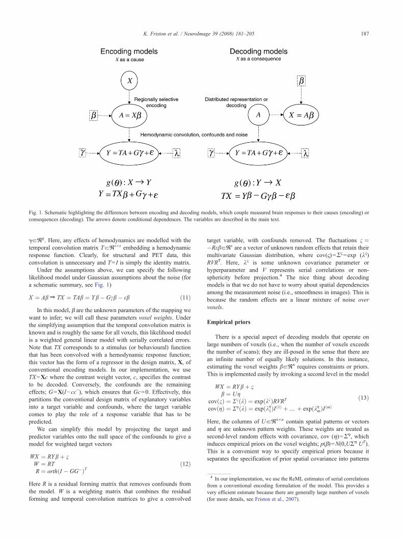
Fig. 1. Schematic highlighting the differences between encoding and decoding models, which couple measured brain responses to their causes (encoding) orconsequences (decoding). The arrows denote conditional dependences. The variables are described in the main text.

4 In our implementation, we use the ReML estimates of serial correlationsfrom a conventional encoding formulation of the model. This provides avery efficient estimate because there are generally large numbers of voxels(for more details, see Friston et al., 2007).


gaRg. Here, any effects of hemodynamics are modelled with thetemporal convolution matrix TaRs�s embedding a hemodynamicresponse function. Clearly, for structural and PET data, thisconvolution is unnecessary and T= I is simply the identity matrix.

Under the assumptions above, we can specify the followinglikelihood model under Gaussian assumptions about the noise (fora schematic summary, see Fig. 1)

X ¼ Ab Z TX ¼ TAb ¼ Yb� Gcb� eb ð11ÞIn this model, β are the unknown parameters of the mapping we

want to infer; we will call these parameters voxel weights. Underthe simplifying assumption that the temporal convolution matrix isknown and is roughly the same for all voxels, this likelihood modelis a weighted general linear model with serially correlated errors.Note that TX corresponds to a stimulus (or behavioural) functionthat has been convolved with a hemodynamic response function;this vector has the form of a regressor in the design matrix, X, ofconventional encoding models. In our implementation, we useTX=Xc where the contrast weight vector, c, specifies the contrastto be decoded. Conversely, the confounds are the remainingeffects; G=X(I−cc−), which ensures that Gc=0. Effectively, thispartitions the conventional design matrix of explanatory variablesinto a target variable and confounds, where the target variablecomes to play the role of a response variable that has to bepredicted.

We can simplify this model by projecting the target andpredictor variables onto the null space of the confounds to give amodel for weighted target vectors

WX ¼ RYbþ 1W ¼ RTR ¼ orthðI � GG�ÞT

ð12Þ

Here R is a residual forming matrix that removes confounds fromthe model. W is a weighting matrix that combines the residualforming and temporal convolution matrices to give a convolved

target variable, with confounds removed. The fluctuations 1 ¼�RebaRs are a vector of unknown random effects that retain theirmultivariate Gaussian distribution, where cov(ς)=Σς=exp (λς)RVRT. Here, λς is some unknown covariance parameter orhyperparameter and V represents serial correlations or non-sphericity before projection.4 The nice thing about decodingmodels is that we do not have to worry about spatial dependenciesamong the measurement noise (i.e., smoothness in images). This isbecause the random effects are a linear mixture of noise overvoxels.

Empirical priors

There is a special aspect of decoding models that operate onlarge numbers of voxels (i.e., when the number of voxels exceedsthe number of scans); they are ill-posed in the sense that there arean infinite number of equally likely solutions. In this instance,estimating the voxel weights baRn requires constraints or priors.This is implemented easily by invoking a second level in the model

WX ¼ RYbþ 1b ¼ Ug

covð1Þ ¼ R1ðkÞ ¼ expðk1ÞRVRT

covðgÞ ¼ RgðkÞ ¼ expðkg1ÞI ð1Þ þ N þ expðkgmÞI ðmÞð13Þ

Here, the columns of UaRn�u contain spatial patterns or vectorsand η are unknown pattern weights. These weights are treated assecond-level random effects with covariance, cov (η)=Ση, whichinduces empirical priors on the voxel weights; p(β)=N(0,UΣη UT).This is a convenient way to specify empirical priors because itseparates the specification of prior spatial covariance into patterns


encoded by U and the variances in the leading diagonal matrix,Ση. In this model, Ση(λ) is a mixture of covariance componentsarising from a nested set of pattern weights, s(1)⊃ s(2)⊃ s(3)⊃…where each subset has the same variance. The ith subset s(i) isencoded by a leading diagonal matrix, I(i), containing dummy orswitch variables indicating which patterns or columns of U belongto that subset. The construction of this nested set means that thevariance; exp(λ1

η)+…+exp(λiη) of a pattern weight in s(i) is always

greater than a pattern weight in its superset, s(i−1).There are many priors that one could specify with this model, one

common prior, used implicitly in fMRI, is that spatial patternscontribute sparsely to the decoding. In other words, a few voxels (orpatterns) have large values of β, while most have small values. Thisis the underlying rationale for support vector machines that pre-suppose only a few data features (support vectors) are needed forclassification. Relevance vector machines make this prior explicit,by framing the elimination of redundant vectors in terms ofempirical priors on the parameters. Relevance vector machines are aspecial case of automatic relevance determination, which is itself aspecial case of variational Bayes. In fact, these special cases can beexpressed formally in terms of conventional expectation maximisa-tion (EM; Dempster et al., 1977), which, for linear models, isformally related to restricted maximum likelihood (ReML; Harville,1977). See Friston et al. (2007) and references therein (e.g., Mackayand Takeuchi, 1996; Tipping, 2001). In this paper, optimisation isformulated in terms of expectation maximisation.

The model above allows us to compare a wide range of spatialmodels for decoding. Sparsity is accommodated by having morethan one subset; where most subsets have small variance and somehave large variance. Crucially, we can control what is sparse. IfU= I is the identity matrix, the spatial vectors encode single voxelsand we have the opportunity to model sparse representations overanatomical regions. This deployment would be consistent withfunctional segregation. Furthermore, we could assume that thissegregation is spatially coherent (for a theoretical motivation interms of neuronal computation, see Friston et al., 1992a,b); thiswould entail using smooth vectors with local support. Conversely,we may assume representations are distributed sparsely overpatterns (i.e., one of a small number of patterns is expressed at any

Fig. 2. Taxonomy of different decoding models that are defined by spatial patterns operceptual or behaviour variables.

one time). These patterns could be the principal modes of co-variation in the data. This would correspond to making U the majorsingular vectors of the data, as in the constrained CCA of theprevious section. Finally, these patterns may simply be the patternsexpressed from moment to moment. In other words, U=YT; this isthe model used in [linear] support vector machines and regression;in fact, these images may contain confounds, which speak to theuse of adjusted images U=RYT. Fig. 2 lists the various modelsconsidered in this paper and the corresponding spatial patterns inU. Models with spatial and smooth vectors imply anatomicallysparse representations. Conversely, models with singular or supportvectors imply the representation is distributed over patterns (whichmay be sparse in pattern space but not sparse anatomically, invoxel space). The key thing about the hierarchal decoding modelabove is that it can accommodate different hypotheses about spatialcoding. These hypotheses can be compared using Bayesian modelcomparison; provided we can evaluate the marginal likelihood ofeach model. In the next section, we describe this evaluation.

Evaluating the marginal likelihood

In what follows, we describe a simple inversion of the model inEq. (13) using conventional EM, under sparse priors on theparameters. This can be regarded as a generalisation of classifica-tion schemes used currently for fMRI, in which the nature of thepriors becomes explicit. This inversion uses standard techniquesand furnishes the log-evidence or marginal likelihood of the modelitself and the conditional density of the voxel weights or decodingparameters. The former can be used to infer on mappings betweenbrain states and their consequences, using model comparison. Thelatter can be used to construct posterior probability maps showingwhich voxels contribute to the decoding, for any particular model.

For a more general and technical discussion of the following,see Friston et al. (2007). In brief, we use a fixed-form variationalapproximation to the approximating posterior under the Laplaceapproximation and the mean field approximation; q(θ)=q(β)q(λ).The Laplace approximation means q(β)=N(μβ,Σβ) and q(λ)=N(μλ,Σλ) are Gaussian and are defined by their conditional meansand covariances. Under these assumptions, the variational scheme

r vectors encoding empirical priors on voxel weights linking brain activity to


reduces to EM. Furthermore, because we can eliminate theparameters β from the generative model (by substituting thesecond level of Eq. (13) into the first), we only need the M-step toestimate q(λ) =N(μλ,Σλ) for model comparison and indeedprediction (cf. Gaussian process modelling). This M-step isformally related to ReML.5

Bayesian inversion with EM

The inversion of Eq. (13) is straightforward because it is asimple hierarchical linear model. Inversion proceeds in two stages:first, hyperparameters encoding the covariances of the error and theempirical prior covariance are estimated in an M-step. Afterconvergence, the conditional moments of the hyperparameters areused to evaluate the conditional moments of the parameters in anE-step and the log-evidence for model comparison. Because we aredealing with a linear model there is no need to iterate the two steps;it is sufficient to iterate the M-step. For simplicity, we will assumethat the pattern sets encoded by I(1),…,I(m) are given and deal withtheir optimisation later.

First, we simplify the model further by eliminating theparameters through substitution

WX ¼ Lgþ 1covðWX Þ ¼ RðkÞ ¼ expðk1ÞQ1 þ N þ expðkmþ1ÞQmþ1

k ¼ fk1; kg1; N ; kgmgQ ¼ fRVRT ; LI ð1ÞLT ; N ; LI ðmÞLTg

ð14Þ

where L=RYU maps the second-level random effects to theweighted target variable. In this form, the only unknown quantitiesare the hyperparameters, λ controlling the covariance Σ(λ) of theweighted target variable. This means we have reduced the problemto optimising the hyperparameters of Σ(λ); this is exactly the formused in Gaussian process modelling.

This covariance includes the covariance of the observationnoise and covariances induced by the second level of the model.w=rank(W) corresponds to the degrees of freedom left afterremoving the effects of confounds. The log-evidence, ln p(X |Y) isapproximated with the free energy (see Eq. (4)):

F ¼ � 12

�XTWTRðμkÞ�1WX � lnjR μk

� �j � wln2pþ lnjΠRkj

� ðμk � pÞTΠ μk � p� �� ð15Þ

The first two terms reflect the accuracy of the model and the lasttwo its complexity (wln2π is a constant). This approximationrequires only the prior p(λ)=N(π,Π−1) and posterior q(λ) =N(μλ,Σλ) densities of the hyperparameters. In our work, we setthe prior expectation and covariance to πi=−32 and Π= I/256,respectively. This is a relatively uninformative hyperprior with asmall expectation. A hyperprior variance of 256 means that a scaleparameter exp(λi) can vary by many orders of magnitude; forexample, a value of 1=exp (0) is two prior standard deviationsfrom the prior mean of 1.26×10−14=exp (−32).

5 This scheme shares formal aspects with relevance vector machines andautomatic relevance determination (e.g., Tipping, 2001); however, thehyperparameters control covariance components as opposed to precisioncomponents. This allows for flexible models through linear mixtures ofcovariance components and renders it an extension of classical covarianceestimation (Harville, 1977).

Note that the free energy also depends on the conditionaluncertainty about the hyperparameters encoded in Σλ. Theconditional moments of the hyperparameters are given by iterating

The M-step

Lki¼ � 12tr Pi WXXTWT � R μk

� �� Πii μki � pi

� �Lkkij¼ � 1

2tr PiRPjR� �� Πij

Dμk¼ �L�1kk Lk

Rk ¼ �L�1kk

ð16Þ

until convergence. This is effectively a Fisher-scoring scheme thatoptimises the free energy bound with respect to the hyper-parameters. It usually takes between four and sixteen iterations(less than a second for a hundred images). Pi=−exp (μi

λ)Σ− 1Qi Σ−1

is the derivative of the precision Σ(μλ)−1, with respect to the ithhyperparameter, evaluated at its conditional expectation. Critically,the computational complexity O(s3m) of this scheme does not scalewith the number of voxels or patterns, but the number of patternsubsets, m. This reflects one of the key advantages of hyper-parameterising the covariances (as opposed to precisions); namely,that one can model mixtures of covariances, induced hierarchically,at the lowest (observation) level of the hierarchy.

Given the conditional expectations of the covariance hyper-parameters from the M-step, the conditional mean and expectationof the parameters obtain analytically from

The E-step

μg ¼ MWXμb ¼ Uμg

Rb ¼ UðRgðμkÞ �MLRgðμkÞÞUT

M ¼ RgðμkÞLTRðμkÞ�1

ð17Þ

Where M is a maximum a posteriori projector matrix. This maylook unfamiliar to some readers who work with linear models,because we have used the matrix inversion lemma to suppress largematrices. This remarkably simple EM scheme solves the difficultproblem of inference on massively ill-posed models in a veryefficient fashion; we use this scheme for source reconstruction inill-posed EEG and MEG problems (Mattout et al., 2006). However,the current problem requires us to address a further issue, namelythe optimisation of the partition (i.e., number and composition ofthe subsets) encoded in, I(i). This bring us to the final component ofBayesian decoding

A greedy search on pattern sets

Many schemes that seek a sparse solution, such as relevancevector regression (Bishop and Tipping, 2000), use a top-downstrategy and start with a separate precision hyperparameter for eachpattern or vector. By estimating the conditional precision of eachpattern weight, redundant or irrelevant patterns can be eliminatedsuccessively until a sparse solution emerges. Clearly, this can entailestimating an enormous number of hyperparameters. We take analternative bottom-up approach, which generalises minimum normsolutions. We start with the minimum norm assumption that allpattern weights have the same variance I(1) = I and use theconditional expectations of the pattern weights to create a new

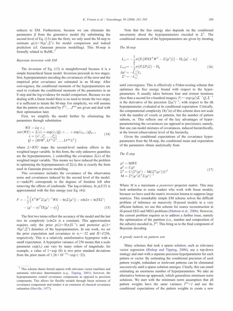
Fig. 3. The EM schemes and its embedding within a greedy search for the optimum set of patterns that maximises the free energy bound on log-evidence. Thevariables are defined in the main text.


subset; with the highest [absolute] values. We then repeat the EMusing two subsets. The subset of patterns with high weights is splitagain to create a new subset and the procedure repeated until thelog-evidence stops increasing (or the mth partition contains asubset with just one pattern). This can be expressed formally as

I ðmþ1Þ ¼ I ðmÞ1jμgjzjμðmÞj ð18Þwhere μ (m) is the median of the conditional pattern weights of themth subset. The “and” operator ∧ ensures that the new set is asubset of the previous set. The result is a succession of smallersubsets, each containing patterns with a higher covariances andweights, which is necessarily sparse. Clearly, if the underlyingweights are not sparse the search will terminate with a smallnumber of subsets and the solution will not be sparse. Thisoptimisation of subsets corresponds to a greedy search: a greedyalgorithm uses the meta-heuristic of making the locally optimumchoice with the hope of finding the global optimum. Greedyalgorithms produce good solutions on some problems, but not all.Most problems for which they work well have optimalsubstructure, which is satisfied in this case, at least heuristically.This is because the problem of finding a subset of patterns withhigh variance can be reduced to finding a bipartition that containsa subset. This is assured, provided we always select a subset withthe highest pattern weights. The result of the greedy search is asparse solution over patterns; where those patterns can beanatomically sparse or distributed. See Fig. 3 for a schematicsummary of the scheme.

In principle,6 adding a subset will either increase the freeenergy or leave it unchanged. This is because each new subset

6 Ignoring problems of local minima.

must, by construction, have a variance that is greater than or equalto its superset. Once the optimal set size is attained, any furthersubsets will have a vanishingly small variance scale-parameter andthe corresponding hyperparameter will tend to its prior expectation;μiλ→πi. In this instance, the curvature approaches the prior

precision, Lλλii→−Πii (see Eq. (16)). This means the conditionalcovariance approaches the prior covariance, which provides anupper bound. It can be seen from Eq. (15) that the free energy isunchanged under these conditions and the subset is effectivelyswitched off. This is an example of automatic model selectiondiscussed in Friston et al. (2007).

Unlike SVM and related automatic relevance determination(ARD) procedures, Bayesian decoding does not eliminateirrelevant patterns. All the patterns are retained during theoptimisation, although some subsets can be switched off asmentioned above. There is no need to eliminate patterns becausethe computational complexity grows with the log of the number ofdata features; O(s3ln(n)). This is because m subsets cover 2m

patterns. This means typically, the greedy search takes a fewseconds, even for thousands of voxels.

Summary

In summary:

• We can formulate a MVB decoding model that maps many datafeatures to a target variable, as a simple hierarchal model; knownas a parametric empirical Bayes model (PEB; Efron and Morris,1973; Kass and Steffey, 1989). The hierarchical structureinduces empirical priors on the data features (i.e., voxels)which we can prescribe in terms of patterns over features. Each


pattern is assigned to a subset of patterns, whose pattern weights(unknown parameters of the mapping) have the same variance.

• Each prescription of patterns (i.e., partition) constitutes ahypothesis about the nature of the mapping between voxelsand the target variable (i.e., the neuronal representation orcause). One can select among competing hypotheses usingmodel selection based on the model evidence. This evidence canbe evaluated quickly using standard variational techniques;formulated as covariance component estimation using EM.

• The partition can be optimised using a greedy search that startswith a classical minimum norm solution and iterates the EMscheme with successive bipartitions of the subset with the largestpattern weights. The free energy or log-evidence of successivepartitions ormodels increases until the optimum set size is reached.

This concludes the specification of the model and its inversion.In the next section, we turn to applications and illustrate the natureof inference entailed by Bayesian decoding.

Illustrative analyses

This section illustrates Bayesian decoding using syntheticand real data. We start with a simple example to show how thegreedy search works. This uses simulated data generated byanatomically sparse representations. We then analyse these data toshow how the log-evidence (or its free energy bound) can be usedto compare models of anatomically sparse and distributed coding.We will analyse three sets of synthetic data (sparse, distributed andnull) with three models (spatial, singular and null) and ensure thatthe inversion scheme identifies the correct model in all cases. Anull model is one in which there are no patterns and no mapping.The simulations conclude with a comparative evaluation of MVBwith a conventional linear discriminant analysis. The focus here ison the increased power of hierarchical models, over classicalmodels that do not employ empirical priors.

We then apply the same models to real data obtained during astudy of attention to visual motion. The emphasis here is on model

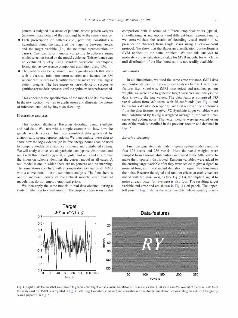
Fig. 4. Right: Data features that were mixed to generate the target variable in the simthe analysis of real fMRI data reported in Fig. 8. Left: Target variable (solid line) andsearch (reported in Fig. 5).

comparison both in terms of different empirical priors (spatial,smooth, singular and support) and different brain regions. Finally,we cross-validate the results of decoding visual motion (i.e.,presence or absence) from single scans using a leave-one-outprotocol. We show that the Bayesian classification out-performs aSVM applied to the same problem. We use this analysis tomotivate a cross-validation p-value for MVB models, for which thenull distribution of the likelihood ratio is not readily available.

Simulations

In all simulations, we used the same error variance, fMRI dataand confounds used in the empirical analyses below. Using thesefeatures (i.e., voxel-wise fMRI time-series) and assumed patternweights we were able to generate target variables and analyse thedata knowing the true values. The data features comprised 583voxel values from 360 scans, with 26 confounds (see Fig. 4 andbelow for a detailed description). We first removed the confoundsfrom the data features to give, RY. Synthetic target variables werethen constructed by taking a weighted average of the voxel time-series and adding noise. The voxel weights were generated usingone of the models described in the previous section and depicted inFig. 2.

Bayesian decoding

First, we generated data under a sparse spatial model using thefirst 128 scans and 256 voxels. Here the voxel weights weresampled from a normal distribution and raised to the fifth power, tomake them sparsely distributed. Random variables were added tothe ensuing target variable after they were scaled to give a signal tonoise of four; i.e., the standard deviation of signal was four timesthe noise. Because the signal and random effects at each voxel aremixed with the same weights (see Eq. (11)), the implicit signal tonoise at each voxel (on average) is also four. The resulting targetvariable and error and are shown in Fig. 4 (left panel). The upper-left panel in Fig. 5 shows the voxel weights, whose sparsity is self-

ulations. These are a subset (128 scans and 256 voxels) of the voxel data fromnoise (broken line) for the simulation demonstrating the nature of the greedy

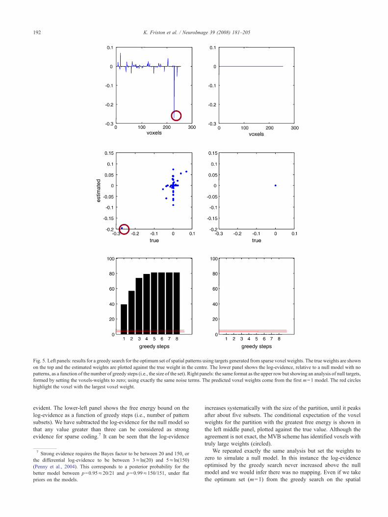
Fig. 5. Left panels: results for a greedy search for the optimum set of spatial patterns using targets generated from sparse voxel weights. The true weights are shownon the top and the estimated weights are plotted against the true weight in the centre. The lower panel shows the log-evidence, relative to a null model with nopatterns, as a function of the number of greedy steps (i.e., the size of the set). Right panels: the same format as the upper row but showing an analysis of null targets,formed by setting the voxels-weights to zero; using exactly the same noise terms. The predicted voxel weights come from the first m=1 model. The red circleshighlight the voxel with the largest voxel weight.


evident. The lower-left panel shows the free energy bound on thelog-evidence as a function of greedy steps (i.e., number of patternsubsets). We have subtracted the log-evidence for the null model sothat any value greater than three can be considered as strongevidence for sparse coding.7 It can be seen that the log-evidence

7 Strong evidence requires the Bayes factor to be between 20 and 150, orthe differential log-evidence to be between 3≈ ln(20) and 5≈ ln(150)(Penny et al., 2004). This corresponds to a posterior probability for thebetter model between p=0.95≈20/21 and p=0.99≈150/151, under flatpriors on the models.

increases systematically with the size of the partition, until it peaksafter about five subsets. The conditional expectation of the voxelweights for the partition with the greatest free energy is shown inthe left middle panel, plotted against the true value. Although theagreement is not exact, the MVB scheme has identified voxels withtruly large weights (circled).

We repeated exactly the same analysis but set the weights tozero to simulate a null model. In this instance the log-evidenceoptimised by the greedy search never increased above the nullmodel and we would infer there was no mapping. Even if we takethe optimum set (m=1) from the greedy search on the spatial


model, the estimated weights are appropriately small (see rightpanels in Fig. 5).

Model comparison

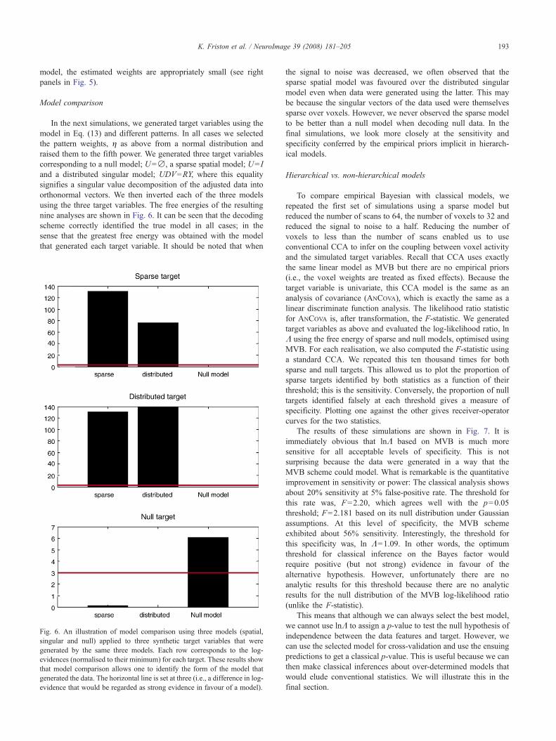
In the next simulations, we generated target variables using themodel in Eq. (13) and different patterns. In all cases we selectedthe pattern weights, η as above from a normal distribution andraised them to the fifth power. We generated three target variablescorresponding to a null model; U=∅, a sparse spatial model; U= Iand a distributed singular model; UDV=RY, where this equalitysignifies a singular value decomposition of the adjusted data intoorthonormal vectors. We then inverted each of the three modelsusing the three target variables. The free energies of the resultingnine analyses are shown in Fig. 6. It can be seen that the decodingscheme correctly identified the true model in all cases; in thesense that the greatest free energy was obtained with the modelthat generated each target variable. It should be noted that when

Fig. 6. An illustration of model comparison using three models (spatial,singular and null) applied to three synthetic target variables that weregenerated by the same three models. Each row corresponds to the log-evidences (normalised to their minimum) for each target. These results showthat model comparison allows one to identify the form of the model thatgenerated the data. The horizontal line is set at three (i.e., a difference in log-evidence that would be regarded as strong evidence in favour of a model).

the signal to noise was decreased, we often observed that thesparse spatial model was favoured over the distributed singularmodel even when data were generated using the latter. This maybe because the singular vectors of the data used were themselvessparse over voxels. However, we never observed the sparse modelto be better than a null model when decoding null data. In thefinal simulations, we look more closely at the sensitivity andspecificity conferred by the empirical priors implicit in hierarch-ical models.

Hierarchical vs. non-hierarchical models

To compare empirical Bayesian with classical models, werepeated the first set of simulations using a sparse model butreduced the number of scans to 64, the number of voxels to 32 andreduced the signal to noise to a half. Reducing the number ofvoxels to less than the number of scans enabled us to useconventional CCA to infer on the coupling between voxel activityand the simulated target variables. Recall that CCA uses exactlythe same linear model as MVB but there are no empirical priors(i.e., the voxel weights are treated as fixed effects). Because thetarget variable is univariate, this CCA model is the same as ananalysis of covariance (ANCOVA), which is exactly the same as alinear discriminate function analysis. The likelihood ratio statisticfor ANCOVA is, after transformation, the F-statistic. We generatedtarget variables as above and evaluated the log-likelihood ratio, lnΛ using the free energy of sparse and null models, optimised usingMVB. For each realisation, we also computed the F-statistic usinga standard CCA. We repeated this ten thousand times for bothsparse and null targets. This allowed us to plot the proportion ofsparse targets identified by both statistics as a function of theirthreshold; this is the sensitivity. Conversely, the proportion of nulltargets identified falsely at each threshold gives a measure ofspecificity. Plotting one against the other gives receiver-operatorcurves for the two statistics.

The results of these simulations are shown in Fig. 7. It isimmediately obvious that lnΛ based on MVB is much moresensitive for all acceptable levels of specificity. This is notsurprising because the data were generated in a way that theMVB scheme could model. What is remarkable is the quantitativeimprovement in sensitivity or power: The classical analysis showsabout 20% sensitivity at 5% false-positive rate. The threshold forthis rate was, F=2.20, which agrees well with the p=0.05threshold; F=2.181 based on its null distribution under Gaussianassumptions. At this level of specificity, the MVB schemeexhibited about 56% sensitivity. Interestingly, the threshold forthis specificity was, ln Λ=1.09. In other words, the optimumthreshold for classical inference on the Bayes factor wouldrequire positive (but not strong) evidence in favour of thealternative hypothesis. However, unfortunately there are noanalytic results for this threshold because there are no analyticresults for the null distribution of the MVB log-likelihood ratio(unlike the F-statistic).

This means that although we can always select the best model,we cannot use lnΛ to assign a p-value to test the null hypothesis ofindependence between the data features and target. However, wecan use the selected model for cross-validation and use the ensuingpredictions to get a classical p-value. This is useful because we canthen make classical inferences about over-determined models thatwould elude conventional statistics. We will illustrate this in thefinal section.

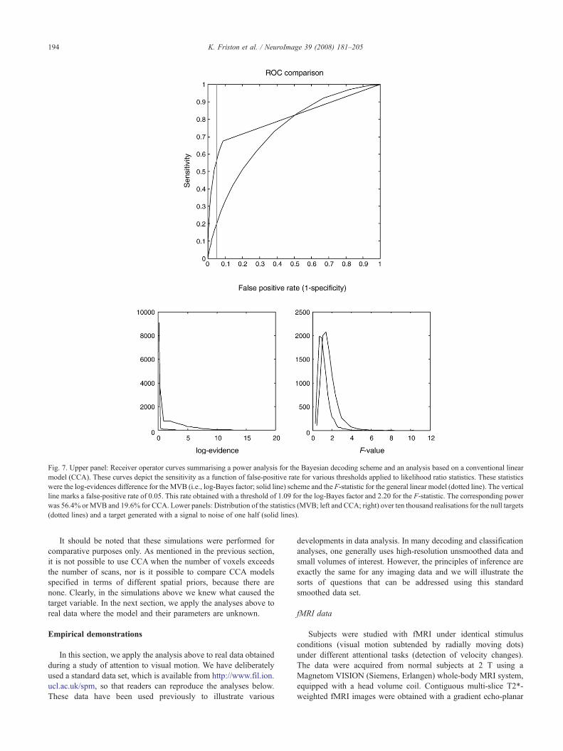
Fig. 7. Upper panel: Receiver operator curves summarising a power analysis for the Bayesian decoding scheme and an analysis based on a conventional linearmodel (CCA). These curves depict the sensitivity as a function of false-positive rate for various thresholds applied to likelihood ratio statistics. These statisticswere the log-evidences difference for the MVB (i.e., log-Bayes factor; solid line) scheme and the F-statistic for the general linear model (dotted line). The verticalline marks a false-positive rate of 0.05. This rate obtained with a threshold of 1.09 for the log-Bayes factor and 2.20 for the F-statistic. The corresponding powerwas 56.4% or MVB and 19.6% for CCA. Lower panels: Distribution of the statistics (MVB; left and CCA; right) over ten thousand realisations for the null targets(dotted lines) and a target generated with a signal to noise of one half (solid lines).


It should be noted that these simulations were performed forcomparative purposes only. As mentioned in the previous section,it is not possible to use CCA when the number of voxels exceedsthe number of scans, nor is it possible to compare CCA modelsspecified in terms of different spatial priors, because there arenone. Clearly, in the simulations above we knew what caused thetarget variable. In the next section, we apply the analyses above toreal data where the model and their parameters are unknown.

Empirical demonstrations

In this section, we apply the analysis above to real data obtainedduring a study of attention to visual motion. We have deliberatelyused a standard data set, which is available from http://www.fil.ion.ucl.ac.uk/spm, so that readers can reproduce the analyses below.These data have been used previously to illustrate various

developments in data analysis. In many decoding and classificationanalyses, one generally uses high-resolution unsmoothed data andsmall volumes of interest. However, the principles of inference areexactly the same for any imaging data and we will illustrate thesorts of questions that can be addressed using this standardsmoothed data set.

fMRI data

Subjects were studied with fMRI under identical stimulusconditions (visual motion subtended by radially moving dots)under different attentional tasks (detection of velocity changes).The data were acquired from normal subjects at 2 T using aMagnetom VISION (Siemens, Erlangen) whole-body MRI system,equipped with a head volume coil. Contiguous multi-slice T2*-weighted fMRI images were obtained with a gradient echo-planar

http://www.fil.ion.ucl.ac.uk/spm



sequence (TE=40 ms, TR=3.22 s, matrix size=64×64×32, voxelsize 3×3×3 mm). The subjects had four consecutive hundred-scansessions comprising a series of ten-scan blocks under five differentconditions D F A F N F A F N S. The first condition (D) was adummy condition to allow for magnetic saturation effects. F(Fixation) corresponds to a low-level baseline where the subjectsviewed a fixation point at the centre of a screen. In condition A(Attention), subjects viewed 250 dots moving radially from thecentre at 4.7° per second and were asked to detect changes inradial velocity. In condition N (No attention) the subjects wereasked simply to view the moving dots. In condition S (Stationary),subjects viewed stationary dots. The order of A and N wasswapped for the last two sessions. In all conditions subjects fixatedthe centre of the screen. In a pre-scanning session the subjectswere given five trials with five speed changes (reducing to 1%).During scanning there were no speed changes. No overt responsewas required in any condition. Data from the first subject are usedhere.

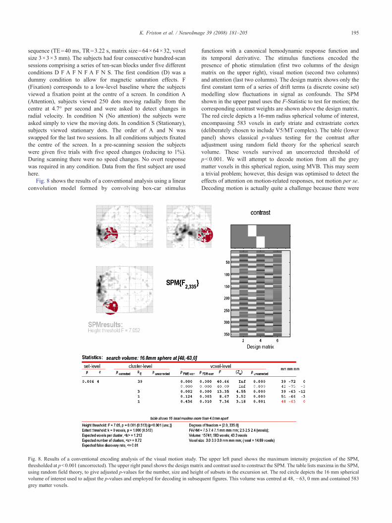
Fig. 8 shows the results of a conventional analysis using a linearconvolution model formed by convolving box-car stimulus

Fig. 8. Results of a conventional encoding analysis of the visual motion study. Tthresholded at pb0.001 (uncorrected). The upper right panel shows the design matriusing random field theory, to give adjusted p-values for the number, size and heighvolume of interest used to adjust the p-values and employed for decoding in subseqgrey matter voxels.

functions with a canonical hemodynamic response function andits temporal derivative. The stimulus functions encoded thepresence of photic stimulation (first two columns of the designmatrix on the upper right), visual motion (second two columns)and attention (last two columns). The design matrix shows only thefirst constant term of a series of drift terms (a discrete cosine set)modelling slow fluctuations in signal as confounds. The SPMshown in the upper panel uses the F-Statistic to test for motion; thecorresponding contrast weights are shown above the design matrix.The red circle depicts a 16-mm radius spherical volume of interest,encompassing 583 voxels in early striate and extrastriate cortex(deliberately chosen to include V5/MT complex). The table (lowerpanel) shows classical p-values testing for the contrast afteradjustment using random field theory for the spherical searchvolume. These voxels survived an uncorrected threshold ofpb0.001. We will attempt to decode motion from all the greymatter voxels in this spherical region, using MVB. This may seema trivial problem; however, this design was optimised to detect theeffects of attention on motion-related responses, not motion per se.Decoding motion is actually quite a challenge because there were

he upper left panel shows the maximum intensity projection of the SPM,x and contrast used to construct the SPM. The table lists maxima in the SPM,t of subsets in the excursion set. The red circle depicts the 16 mm sphericaluent figures. This volume was centred at 48, −63, 0 mm and contained 583


only four epochs of stationary stimuli (note that the effects ofphotic stimulation are treated as confounds in the decoding model).

Before looking at Bayesian decoding, it is worthwhile notingthat multivariate inference using random field theory suggests themutual information between the voxel time courses and motionis significant. This can be inferred from the set-level inferencewith pb0.006 (left-hand column of the table, Fig. 8). This isbased on the observed number of peaks surviving a pb0.001threshold in the volume of interest. Here we expected 0.72 peaks

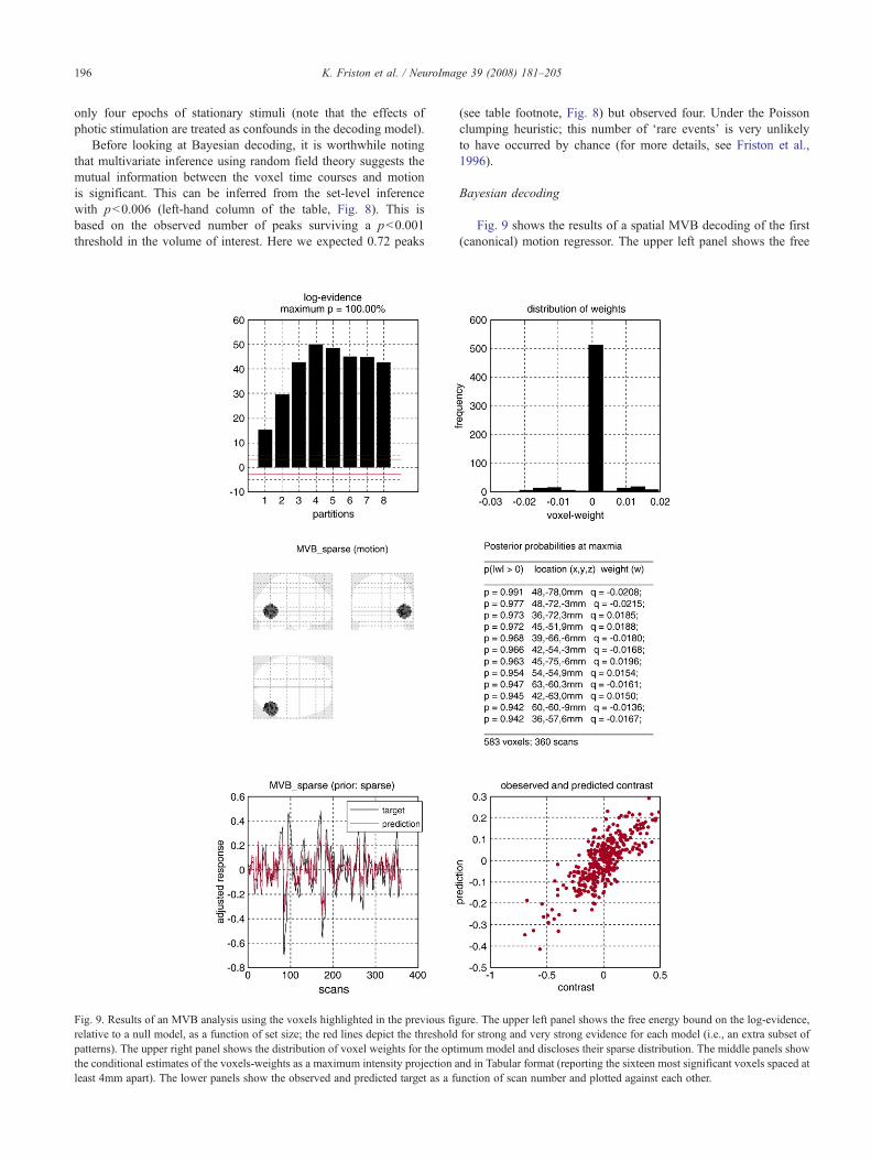
Fig. 9. Results of an MVB analysis using the voxels highlighted in the previous figrelative to a null model, as a function of set size; the red lines depict the thresholdpatterns). The upper right panel shows the distribution of voxel weights for the optthe conditional estimates of the voxels-weights as a maximum intensity projection aleast 4mm apart). The lower panels show the observed and predicted target as a fu

(see table footnote, Fig. 8) but observed four. Under the Poissonclumping heuristic; this number of ‘rare events’ is very unlikelyto have occurred by chance (for more details, see Friston et al.,1996).

Bayesian decoding

Fig. 9 shows the results of a spatial MVB decoding of the first(canonical) motion regressor. The upper left panel shows the free

ure. The upper left panel shows the free energy bound on the log-evidence,for strong and very strong evidence for each model (i.e., an extra subset ofimum model and discloses their sparse distribution. The middle panels shownd in Tabular format (reporting the sixteen most significant voxels spaced atnction of scan number and plotted against each other.

8 Chih-Chung Chang and Chih-Jen Lin, LIBSVM: a library for supportvector machines, 2001. Software available at http://www.csie.ntu.edu.tw/~cjlin/libsvm.


energy approximation to the log-evidence for each of eight greedysteps, having subtracted the log-evidence for the correspondingnull model. As in the previous section, any log-evidence differenceof three or more can be considered strong evidence in favour of themodel. It can be seen that the log-evidence peaks with four subsets,giving an anatomically sparse deployment of voxel weights (upperright panel). This sparsity is evidenced by the heavy tails of thedistribution, lending it a multimodal form. These weights (positivevalues only) are shown as a maximum intensity projection and intabular format in the middle row. The table also provides theposterior probability that the voxel weight is greater or less thanzero (for peaks that are at least 4mm apart). Note that theseprobabilities are conditioned on the model as well as the data. Thatis, under the sparse model with spatial vectors, the probability thatthe first voxel has a weight greater than zero, given the targetvariable, is 99.1%. Note that the free energy decreases after foursubsets. Strictly speaking this should not happen because the freeenergy can only increase or stay the same with extra components.However, in this case, the EM scheme has clearly converged on alocal maximum, when there are too many subsets. This is not anissue in practice, because one would still select the best model,which hopefully is a global maximum.

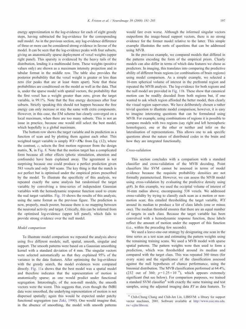
The bottom row shows the target variable and its prediction as afunction of scan and by plotting them against each other. Thisweighted target variable is simply WX=RXc from Eq. (12), wherethe contrast, c, selects the first motion regressor from the designmatrix, X, in Fig. 8. Note that the motion target has a complicatedform because all other effects (photic stimulation, attention andconfounds) have been explained away. The agreement is notsurprising because one could produce a perfect prediction given583 voxels and only 360 scans. The key thing is that the match isnot perfect but is optimised under the empirical priors prescribedby the model. To illustrate the specificity of this analysis, werepeated exactly the same analysis but randomised the targetvariable by convolving a time-series of independent Gaussianvariables with the hemodynamic response function used to createthe real target variables. Fig. 10 shows the results of this analysis,using the same format as the previous figure. The prediction isnow, properly, much poorer, because there is no mapping betweenthe neuronal activity and target. Critically, this can be inferred fromthe optimised log-evidence (upper left panel), which fails toprovide strong evidence over the null model.

Model comparison

To illustrate model comparison we repeated the analysis aboveusing five different models; null, spatial, smooth, singular andsupport. The smooth patterns were based on a Gaussian smoothingkernel with a standard deviation of 4 mm. The singular vectorswere selected automatically so that they explained 95% of thevariance in the data features. After optimising the log-evidencewith the greedy search, the model evidences were compareddirectly. Fig. 11a shows that the best model was a spatial modeland therefore indicates that the representation of motion isanatomically sparse; as one would predict under functionalsegregation. Interestingly, of the non-null models, the smoothvectors were the worst. This suggests that, even though the fMRIdata were smoothed, the underlying representation of motion is notdispersed spatially; again this would be expected under patchyfunctional segregation (see Zeki, 1990). One would imagine that,in the absence of smoothing, the model with smooth patterns

would fare even worse. Although the informed singular vectorsoutperform the image-based support vectors, there is no strongevidence for the former model relative to the latter. This simpleexample illustrates the sorts of questions that can be addressedusing MVB.

In the previous example, we compared models that differed inthe patterns encoding the form of the empirical priors. Clearlymodels can also differ in terms of which data features we chose aspredictors. In imaging, this translates into comparing the predictiveability of different brain regions (or combinations of brain regions)using model comparison. As a simple example, we selected a16-mm spherical volume of interest in the prefrontal region andrepeated the MVB analysis. The log-evidence for both regions andthe null model are provided in Fig. 11b. These show that canonicalmotion can be readily decoded from both regions but, if onewanted to ask which region afforded the better model, then clearlythe visual region supervenes. We have deliberately chosen a rathertrivial question to illustrate model comparison; however, it is easyto imagine interesting questions that can be formulated usingMVB. For example, using combinations of regions it is possible tocompare models with two regions (say right and left hemispherichomologues), one or the other or neither and infer on thelateralisation of representations. This allows one to ask specificquestions about the nature of distributed codes in the brain andhow they are integrated functionally.

Cross-validation

This section concludes with a comparison with a standardclassifier and cross-validation of the MVB decoding. Pointclassifiers like SVM cannot be assessed in terms of modelevidence because the requisite probability densities are notformally parameterised. However, we can assess the MVB modelusing cross-validation by evaluating the predictive density usingq(θ). In this example, we used the occipital volume of interest of16-mm radius above, encompassing 538 voxels. We addressedcross-validity by trying to classify each scan as a motion or non-motion scan; this entailed thresholding the target variable, WXaround its median to produce a list of class labels (one or minusone). The median threshold ensures that there are an equal numberof targets in each class. Because the target variable has beenconvolved with a hemodynamic response function, these labelsreflect the amount of motion under the support of this function(i.e., within the preceding few seconds).

We used a leave-one-out strategy by designating one scan in thetime series as a test scan and estimating the pattern weights usingthe remaining training scans. We used a MVB model with sparsespatial patterns. The pattern weights were then used to form aprediction, which was thresholded around its median andcompared with the target class. This was repeated 360 times (forevery scan) and the significance of the classification assessedagainst the null hypotheses of chance performance, using thebinomial distribution. The MVB classification performed at 64.4%,(232 out of 360; p=1.25×10−8), which appears extremelysignificant (but see below). For comparison purposes, we traineda standard SVM classifier8 with exactly the same training and testsamples, using the adjusted imaging data RY as data features. To

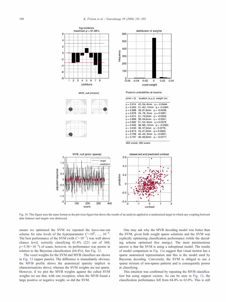
http://www.csie.ntu.edu.tw/~cjlin/libsvm

http://www.csie.ntu.edu.tw/~cjlin/libsvm

Fig. 10. This figure uses the same format as the previous figure but shows the results of an analysis applied to a randomised target in which any coupling betweendata features and targets was destroyed.


ensure we optimised the SVM we repeated the leave-one-outscheme for nine levels of the hyperparameter C=100, …, 10−8.The best performance of the SVM (with C=10−3) was well abovechance level, correctly classifying 61.4% (221 out of 360;p=5.58×10−6) of scans; however, its performance was poorer inrelation to the Bayesian classification (64.4%). See Fig. 12.

The voxel weights for the SVM and MVB classifiers are shownin Fig. 13 (upper panels). The difference is immediately obvious;the MVB profile shows the anatomical sparsity implicit incharacterisations above; whereas the SVM weights are not sparse.However, if we plot the MVB weights against the cubed SVMweights we see that, with one exception, when the MVB found alarge positive or negative weight, so did the SVM.

One may ask why the MVB decoding model was better thanthe SVM, given both sought sparse solutions and the SVM wasexplicitly optimising classification performance (while the decod-ing scheme optimised free energy). The most parsimoniousanswer is that the SVM is using a suboptimal model. The resultsof model comparison in Fig. 11a suggest that visual motion has asparse anatomical representation and this is the model used byBayesian decoding. Conversely, the SVM is obliged to use asparse mixture of non-sparse patterns and is consequently poorerat classifying.

This intuition was confirmed by repeating the MVB classifica-tion but using support vectors. As can be seen in Fig. 12, theclassification performance fell from 64.4% to 63.0%. This is still

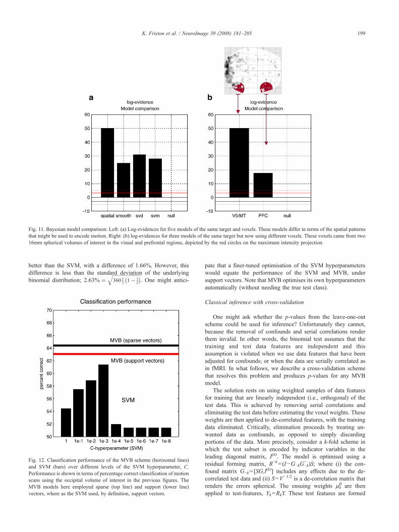
Fig. 11. Bayesian model comparison: Left: (a) Log-evidences for five models of the same target and voxels. These models differ in terms of the spatial patternsthat might be used to encode motion. Right: (b) log-evidences for three models of the same target but now using different voxels. These voxels came from two16mm spherical volumes of interest in the visual and prefrontal regions, depicted by the red circles on the maximum intensity projection.


better than the SVM, with a difference of 1.66%. However, thisdifference is less than the standard deviation of the underlyingbinomial distribution; 2:63% ¼

ffiffiffiffiffiffiffiffiffiffiffiffiffiffiffiffiffiffiffiffiffiffiffiffiffi360 1

2 1� 12

� �q. One might antici-

Fig. 12. Classification performance of the MVB scheme (horizontal lines)and SVM (bars) over different levels of the SVM hyperparameter, C.Performance is shown in terms of percentage correct classification of motionscans using the occipital volume of interest in the previous figures. TheMVB models here employed sparse (top line) and support (lower line)vectors, where as the SVM used, by definition, support vectors.

pate that a finer-tuned optimisation of the SVM hyperparameterswould equate the performance of the SVM and MVB, undersupport vectors. Note that MVB optimises its own hyperparametersautomatically (without needing the true test class).

Classical inference with cross-validation

One might ask whether the p-values from the leave-one-outscheme could be used for inference? Unfortunately they cannot,because the removal of confounds and serial correlations renderthem invalid. In other words, the binomial test assumes that thetraining and test data features are independent and thisassumption is violated when we use data features that have beenadjusted for confounds; or when the data are serially correlated asin fMRI. In what follows, we describe a cross-validation schemethat resolves this problem and produces p-values for any MVBmodel.

The solution rests on using weighted samples of data featuresfor training that are linearly independent (i.e., orthogonal) of thetest data. This is achieved by removing serial correlations andeliminating the test data before estimating the voxel weights. Theseweights are then applied to de-correlated features, with the trainingdata eliminated. Critically, elimination proceeds by treating un-wanted data as confounds, as opposed to simply discardingportions of the data. More precisely, consider a k-fold scheme inwhich the test subset is encoded by indicator variables in theleading diagonal matrix, I(k). The model is optimised using aresidual forming matrix, R−k=(I−G−kG−k

− )S; where (i) the con-found matrix G−k=[SG,I

(k)] includes any effects due to the de-correlated test data and (ii) S=V−1/2 is a de-correlation matrix thatrenders the errors spherical. The ensuing weights μk

β are thenapplied to test-features, Yk=RkY. These test features are formed

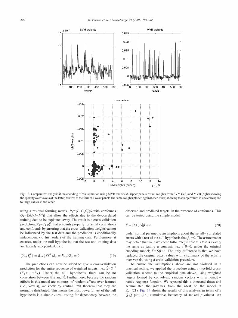
Fig. 13. Comparative analysis if the encoding of visual motion using MVB and SVM. Upper panels: voxel weights from SVM (left) and MVB (right) showingthe sparsity over voxels of the latter, relative to the former. Lower panel: The same weights plotted against each other, showing that large values in one correspondto large values in the other.


using a residual forming matrix, Rk=(I−GkGk−)S with confounds

Gk=[SG,(I− I(k))] that allow the effects due to the de-correlated

training data to be explained away. The result is a cross-validationprediction, Xk=Yk μk

β, that accounts properly for serial correlationsand confounds by ensuring that the cross-validation weights cannotbe influenced by the test data and the prediction is conditionallyindependent (to first order) of the training data. Furthermore, itensures, under the null hypothesis, that the test and training dataare linearly independent; i.e.,

Y�kYTk

� � ¼ R�k YYT� �

Rk ¼ R�kVRk ¼ 0 ð19Þ

The predictions can now be added to give a cross-validationprediction for the entire sequence of weighted targets; i.e., X=S−1

(X1+…+XK). Under the null hypothesis, there can be nocorrelation between WX and X. Furthermore, because the randomeffects in this model are mixtures of random effects over features(i.e., voxels), we know by central limit theorem that they arenormally distributed. This means the most powerful test of the nullhypothesis is a simple t-test; testing for dependency between the

observed and predicted targets, in the presence of confounds. Thiscan be tested using the simple model

X¼ ½TX ;G�bþ e ð20Þ

under normal parametric assumptions about the serially correlatederrors with a test of the null hypothesis that β1=0. The astute readermay notice that we have come full-circle; in that this test is exactlythe same as testing a contrast, i.e., cTβ=0, under the originalencoding model; X=Xβ+ε. The only difference is that we havereplaced the original voxel values with a summary of the activityover voxels, using a cross-validation procedure.

To ensure the assumptions above are not violated in apractical setting, we applied the procedure using a two-fold cross-validation scheme to the empirical data above, using weightedtargets formed by convolving random vectors with a hemody-namic response function. We repeated this a thousand times andaccumulated the p-values from the t-test on the model inEq. (21). Fig. 14 shows the results of this analysis in terms of aQ-Q plot (i.e., cumulative frequency of ranked p-values). An

Fig. 15. Results of a two-fold cross-validation using the motion target andthe 360 scans of 583-voxel features from the visual volume of interest.Upper panel: The target variable (solid line) and its prediction (broken line)from the cross-validation. Lower panel: the same data plotted against eachother. These results can be compared with the lower panels in Fig. 9. Thedifference here is that the prediction of one half of the time-series is based ondata from the other.

Fig. 14. Results of a simulation study to ensure the exact nature of cross-validation p-values. This Q-Q plot shows the cumulative frequency ofranked p-values from one thousand, two-fold cross-validation tests using thedata features from the fMRI study (V5/MT volume of interest) and arandomised weighted target. Ideally the Q-Q plot should be a straight linepassing though the origin. The number of p-values falling below p=0.05was 0.056, suggesting a reasonably exact test.


exact and valid test should produce a straight line though theorigin; happily this is what we observed. This is importantbecause it gives a reasonably powerful test that enables classicalinference about multivariate models for which no conventionalresults exist.

Fig. 15 shows the results of the cross-validation prediction forthe 16-mm occipital volume of interest. This prediction should becompared with that in Fig. 9 that was obtained without the cross-validation constraint. It can be seen that the accuracy of thisprediction is unlikely to have occurred by chance; the correspond-ing cross-validation p-value was p=0.000046 and was extremelysignificant.

Summary

In summary, this section has demonstrated the nature ofinference with MVB. We anticipate that most analyses could useboth Bayesian and classical inference. First, [Bayesian] modelcomparison would be used to identify the best qualitative form ofmodel for any structure–function relationship, using the log-evidence over models. Having established the best model thecross-validation p-value can be used for a quantitative [classical]inference that any dependencies between observed brain mea-sures and their consequences are unlikely to have occurred bychance.

Discussion

This paper has described a multivariate Bayesian (MVB)scheme to decode neuroimages. This scheme resolves the ill-

posed many-to-one mapping, from voxels or data features to atarget variable, using a parametric empirical Bayesian modelwith covariance hyperpriors. This model is inverted usingexpectation maximisation to furnish the model evidence andthe conditional density of the parameters of each model. Thisallows one to compare different models or hypotheses about themapping from functional or structural anatomy to perceptual andbehavioural consequences (or their deficits). The primary aim ofMVB is not to predict or classify these consequences but toenable inference on different models of structure–function


mappings; such as the distinction between distributed and sparserepresentations. This allows one to optimise the model itself andproduce predictions that can outperform standard pattern clas-sification approaches.

MVB is a model comparison approach that is well suited fortesting specific hypotheses about structure–function mappings;e.g., is the representation of objects sparse or distributed in thevisual cortex? The outputs of MVB are the log-evidences for themodels tested, which allows inference about spatial coding and theconditional density of the voxel weights. In addition, one can alsoderive a cross-validation p-value for MVB models. On the otherhand, classifier approaches like support vector machines (SVM)optimise the parameters of a discriminating function to maximiseclassification accuracy. They are useful when one wants to makepredictions about new examples, especially when there is no priorhypothesis available or the model assumptions can not beguaranteed (e.g., classifying patients vs. controls, predictingtreatment response, predicting subject decisions about novelstimuli, etc.). The outputs of this approach are the classificationaccuracy and the voxel weights.

Model inversion and inference in MVB uses exactly the sameempirical Bayesian procedures developed for ill-posed inverseproblems (e.g., source reconstruction in EEG). However, theMVB scheme extends this approach to include an efficient greedysearch for sparse solutions. In contradistinction to top-downstrategies, employed by things like automatic relevance determi-nation, MVB uses a computationally expedient bottom-up searchfor the optimum partition; i.e., number and composition of patternweight subsets with the same variance. It should be noted thatthere is a distinction between the abstraction of model comparisonas the computation of a metric (e.g., likelihood ratio) and a searchalgorithm (e.g., greedy search). One reason to make thisdistinction lies in the need to consider when a particular searchalgorithm is appropriate; for example, a greedy search may besuitable for our purposes, in optimising linear models, yet may failfor nonlinear multivariate associations (e.g., the exclusive- or(XOR) association that eluded early neural-network solutionalgorithms).

We have illustrated MVB using simulated and real data, with aspecial focus on model comparison; where models can differ in theform of the mapping (i.e., neuronal representation) within oneregion, or in terms of the regions themselves. These demonstra-tions concluded with a procedure to compute exact p-values forclassical inference on the model selected, using cross-validation.We organise the rest of the discussion around some obviousquestions; many of which have been posed by colleagues afterdiscussing the material above.

Can one use Bayesian decoding with event-related fMRIparadigms?

Yes. In fact the scheme can be applied to any data and designthat can be formulated as a conventional linear model. Thisincludes convolution models for fMRI studies with efficientdesign. Unlike classification schemes, the model does not map toclasses or labels, but to continuous, real-valued target variables;therefore, one is not forced to assign each scan to a class.Furthermore, the target variable is convolved by a hemodynamicresponse so that the delay and dispersion inherent in fMRImeasures of neuronal activity becomes an explicit part of thedecoding.

Does the scheme assume the same hemodynamic response functionin all voxels?

Not if variations in voxel-specific hemodynamic responsefunctions are included as confounds. For example, to a first-orderapproximation, one can model differences in hemodynamic latencywith the temporal derivative of the target variable (and any otherconfounds). This derivative enters the projection matrix, R, whicheffectively removes variations in latency in both the target variableand voxel time series. Similar arguments apply to other variationsin the response function. In practice, decoding uses exactly thesame model specification as encoding. The target variable isspecified with contrast weights in the usual way but they are usedto subtract the corresponding column (or mixture of columns) fromthe design matrix. This reduced design matrix now becomes theconfound matrix in a decoding model and will contain regressorsnecessary for explaining away differences in hemodynamicresponses (provided a suitable basis set was specified for theconventional analysis).

Can MVB be applied to structural images or contrasts inmulti-subject studies?

Yes. As mentioned above, it can be used in any context thatlends itself to conventional modelling. This includes the analysisof grey matter segments in voxel-based morphometry. Thismeans it is possible to infer on structure–function mappingsexplicitly; for example one can use grey matter segments from agroup to predict neuropsychological deficit, diagnosis orresponse to treatment. In fact, this application was one of theprimary motivations for this work (see below).

Can the scheme cope with serial correlations in the errors?

Yes. These can be accommodated by adding extra errorcovariance components modelling any non-sphericity. The asso-ciated hyperparameter will be estimated in the EM scheme alongwith the others. In the current implementation, this is not necessarybecause we use the serial correlations V from a conventionalanalysis using ReML.

Is a greedy search for a sparse solution appropriate if the neuronalrepresentation is not sparse (i.e., if it is distributed)?

Yes. A sparse solution in the space of pattern weights does notmean the solution is anatomically sparse because the patterns can besparse or distributed. Both the hyperpriors and greedy search canaccommodate sparse solutions in the space of pattern weights. Thissparsity is a useful constraint on the many-to-one nature of thedecoding problem; it means the scheme will seek an optimumsparse solution for any set of patterns that are specified. However,the patterns that model the anatomical deployment of neuronalactivity may or may not be sparse. This means one can infer arepresentation is distributed by comparing two models with sparse(e.g., spatial vectors) and non-sparse (e.g., support vectors) patterns.

Will the greedy search find significant subsets when there is nomapping?

No. The free energy bound that is optimised by both the greedysearch, and each iteration of the EM scheme, embodies both

9 The symbol⊗ means Kronecker tensor product and is equivalent takingall the products of elements in two vectors (or matrices).


accuracy and complexity. This means that adding a hyperparameterto the model will only increase the bound, if the increase inaccuracy (i.e., fit) more than compensates for increased modelcomplexity. This is why the log-evidence did not exceed the nullmodel during the greedy search, using the null data in thesimulations (see Fig. 5).

Why does Bayesian inference not use cross-validation likeclassification schemes?

Because it does not need to; classification schemes aregenerally obliged to use cross-validation or generalisation errorto assess how good they are because they do not furnishinference on the mapping they are trying to model. Makinginferences with classification still rests on model comparison butdoes so only at the last step, where one compares classificationperformance with a null model of chance classification (e.g.,using a binomial distribution). From the perspective of modelcomparison, classification performance is a surrogate for thelikelihood ratio. We exploited this approach to compute a p-value for classical inference using cross-validation.

Can the Bayesian decoding model be used to classify?

Generally, if a model is to be applied to classificationproblems, where the class labels are discrete, one usually useslogistic or multinomial regression, where the log-likelihood ratiois a linear function of some parameters. These models are basedon binomial/multinomial distributions, as opposed to theGaussian densities used in MVB. However, the continuoustarget variables, assumed by MVB, can be thresholded to givedistinct classes or labels (for an example, see the comparisonbetween MVB and SVM above). Having said this, the objectiveof Bayesian decoding is more general and is not simply toestablish a statistical dependency between neuronal representa-tions and a perceptual or behavioural consequences; it is con-cerned with comparing different models of that mapping. This isnot possible with simple classification because classificationschemes use only one model (the model that has been optimisedwith respect to generalisation error). Classification is therefore aspecial application of the more general MVB framework pre-sented here.

We conclude with a brief review of extensions of the linearmodel presented here. These include nonlinear models andextensions to cover multiple target variables.

Nonlinear models

As mentioned above, we envisage applying this sort ofanalysis to look at structure–function relationships in the brain,using structural images (e.g., grey matter segments frommultiple subjects). An important application here is lesion-deficit analysis, where one wants to understand how damage todifferent brain areas conspires to provide a behavioural deficit.A critical aspect of this mapping is that is may be nonlinear. Inother words, the production of a deficit following damage toone region depends on the integrity of another (as indegenerate structure–function mappings). We have emphasisedthe necessary role of multivariate models in this contextpreviously, when qualifying the use of voxel-based morpho-metry (Friston and Ashburner, 2004). There have been some

exciting developments in this context; using directed Bayesiangraphs (see Herskovits and Gerring, 2003). In the context ofour parametric model, nonlinearities are easy to include,through the use of polynomial expansions. For example,9

WX ¼ Ry1U y1U � y1Uv v

ysU ysU � ysU

24

35 g1

g2

þ 1 ð21Þ

can be treated as in exactly the same way as the first-ordermodel above to provide the log-evidence and conditionalestimates of the first and second-order pattern weights; η1 andη2. The first-order weights play exactly the same role aspreviously; however, the second-order weights model interac-tions between patterns in causing the target. An importantexample of this is predicting a psychological deficit by damageto two regions that have a degenerative (many-to-one)structure–function relationship (see Price and Friston, 2002).Under second-order degeneracy, a deficit would not be evidentin damage to either region alone and would require a non-zerosecond-order weight on bilateral regional damage to predict adeficit. In principle, one could establish second-order degen-eracy by comparing the second-order model above to itsreduced first-order form.

WX ¼ Ry1Uv

ysU

24

35g1 þ 1 ð22Þ

which is exactly the same as Eq. (13). We will exploitnonlinear MVB in future work on multi-lesion deficit analysesof structural scans.

Comparing different representations

This paper has dealt with the simple case, where X is univariate(e.g., a subspace of a fuller design, specified with one-dimensionalcontrast). The more general case of multivariate decoding entailsexactly the same formulation but with vectorised variables. Animportant example of this would be models for two contrasts ortargets (e.g., house and face perception). A model for twoperceptual targets X1 and X2 is

W1X1

W2X2

¼ R1Y �R1Y

R2Y R2Y

UgðþÞ

Ugð�Þ

þ 11

12

ð23Þ

This model has the same form as Eq. (13) but has been arrangedso that the pattern weights η(+) map activity in patterns to bothtargets, whereas η(−) map differential activity to the target. Thismeans that η(+) are weights that mediate overlapping representa-tions and η(−) determine which patterns or voxels predict the targetsuniquely. Note that the errors are uncorrelated because they aremixture of orthogonal voxel weights. By comparing this full modelwith a reduced model

W1X1

W2X2

¼ �R1Y

R2Y

Ugð�Þ þ 11

12

1 ð24Þ

one should be able to test for common or overlapping representa-tions and disambiguate between category-specific representations


that are functionally selective (with overlap) and functionallysegregated (without). We will explore this in future work.

Software note

The Bayesian decoding scheme, described in this paper, willbe available in the next release of SPM5 (http://www.fil.ion.ucl.ac.uk/spm). It is accessed through the results panel (multivariateBayes) after displaying a contrast as an SPM. It is assumed thatthe target variable is the compound or contrast of regressorsspecified by the contrast weights of the SPM. If an F-contrast isspecified, the first component is used for decoding. The volumeof interest is specified in the usual way (sphere, box or mask)and the greedy search is initiated for the model (spatial, smooth,singular or sparse) requested. After the model has beenoptimised or selected its cross-validation p-value can be accessedusing a two-fold scheme illustrated in the main text. The resultsare displayed using the same format used (Figs. 9, 10 and 15)above.

Acknowledgments

The Wellcome Trust funded this work. This work wasundertaken under the auspices of the Brain Network RecoveryGroup (http://www.brainnrg.org), sponsored by the James S.McDonnell Foundation.

References

Ashburner, J., Friston, K.J., 2005. Unified segmentation. NeuroImage 26(3), 839–851.

Beal, M.J., 1998. Variational algorithms for approximate Bayesian in-ference; PhD Thesis: http://www.cse.buffalo.edu/faculty/mbeal/thesis/,p. 58.

Bishop, C.M., Tipping, M.E., 2000. Variational relevance vector machines.In: Boutilier, C., Goldszmidt, M. (Eds.), Proceedings of the 16thConference on Uncertainty in Artificial Intelligence. Morgan Kaufmann,pp. 46–53.

Büchel, C., Holmes, A.P., Rees, G., Friston, K.J., 1998. Characterizingstimulus-response functions using nonlinear regressors in parametricfMRI experiments. NeuroImage 8 (2), 140–148.

Carlson, T.A., Schrater, P., He, S., 2003. Patterns of activity in the categoricalrepresentations of objects. J. Cogn. Neurosci. 15 (5), 704–717.

Cox, D.D., Savoy, R.L., 2003. Functional magnetic resonance imaging(fMRI) “brain reading”: detecting and classifying distributed patternsof fMRI activity in human visual cortex. NeuroImage 19 (2 Pt. 1),261–270.

Dempster, A.P., Laird, N.M., 1977. Maximum likelihood from incompletedata via the EM algorithm. J. R. Stat. Soc., Ser. B Stat. Methodol. 39,1–38.

Efron, B., Morris, C., 1973. Stein’s estimation rule and its competitors—Anempirical Bayes approach. J. Am. Stat. Assoc. 68, 117–130.

Feynman, R.P., 1972. Statistical Mechanics. Benjamin, Reading MA, USA.Friman, O., Cedefamn, J., Lundberg, P., Borga, M., Knutsson, H., 2001.

Detection of neural activity in functional MRI using canonical cor-relation analysis. Magn. Reson. Med. 45 (2), 323–330.

Friston, K.J., 2007. Linear models and inference. In: Friston, K.J.,Ashburner, J.T., Kiebel, S.J., Nichols, T.E., Penny, W.D. (Eds.),Statistical Parametric Mapping. Academic Press, London, pp. 589–591.

Friston, K.J., Ashburner, J., 2004. Generative and recognition models forneuroanatomy. NeuroImage 23 (1), 21–24.

Friston, K.J., Liddle, P.F., Frith, C.D., Hirsch, S.R., Frackowiak, R.S.,1992a. The left medial temporal region and schizophrenia. A PET study.Brain 115 (Pt 2), 367–382.

Friston, K.J., Frith, C.D., Passingham, R.E., Dolan, R.J., Liddle, P.F.,Frackowiak, R.S., 1992b. Entropy and cortical activity: informationtheory and PET findings. Cereb. Cortex 2 (3), 259–267.

Friston, K.J., Frith, C.D., Frackowiak, R.S., Turner, R., 1995. Characterizingdynamic brain responses with fMRI: a multivariate approach. Neuro-Image 2 (2), 166–172.

Friston, K.J., Holmes, A., Poline, J.B., Price, C.J., Frith, C.D., 1996.Detecting activations in PET and fMRI: levels of inference and power.NeuroImage 4, 223–235.

Friston, K.J., Penny, W., Phillips, C., Kiebel, S., Hinton, G., Ashburner, J.,2002. Classical and Bayesian inference in neuroimaging: theory.NeuroImage 16, 465–483.

Friston, K., Mattout, J., Trujillo-Barreto, N., Ashburner, J., Penny, W., 2007.Variational free energy and the Laplace approximation. NeuroImage 34(1), 220–234.

Grady, C.L., Haxby, J.V., Schapiro, M.B., Gonzalez-Aviles, A., Kumar, A.,Ball, M.J., Heston, L., Rapoport, S.I., 1990. Subgroups in dementia ofthe Alzheimer type identified using positron emission tomography.J. Neuropsychiatry Clin. Neurosci. 2 (4), 373–384.

Grunwald, P., Pitt, M.A., Myung, I.J. (Eds.), April 2005. Advances inMinimum Description Length: Theory and Applications. M.I.T. Press(MIT Press).

Hanson, S.J., Matsuka, T., Haxby, J.V., 2004. Combinatorial codes in ventraltemporal lobe for object recognition: Haxby (2001) revisited: is there a“face” area? NeuroImage 23 (1), 156–166.

Harville, D.A., 1977. Maximum likelihood approaches to variancecomponent estimation and to related problems. J. Am. Stat. Assoc. 72,320–338.

Hasson, U., Nir, Y., Levy, I., Fuhrmann, G., Malach, R., 2004. Intersubjectsynchronization of cortical activity during natural vision. Science 303(5664), 1634–1640.

Haynes, J.D., Rees, G., 2005. Predicting the orientation of invisible stimulifrom activity in human primary visual cortex. Nat. Neurosci. 8 (5),686–691.

Haynes, J.D., Rees, G., 2006. Decoding mental states from brain activity inhumans. Nature reviews. Neuroscience 7 (7), 523–534.

Herndon, R.C., Lancaster, J.L., Toga, A.W., Fox, P.T., 1996. Quantificationof white matter and gray matter volumes from T1 parametric imagesusing fuzzy classifiers. J. Magn. Reson. Imaging 6 (3), 425–435.

Herskovits, E.H., Gerring, J.P., 2003. Application of a data-mining methodbased on Bayesian networks to lesion-deficit analysis. NeuroImage 19(4), 1664–1673.

Kamitani, Y., Tong, F., 2006. Decoding seen and attended motion directionsfrom activity in the human visual cortex. Curr. Biol. 16 (11), 1096–1102.

Kass, RE., Raftery, A.E., 1995. Bayes factors. J. Am. Stat. Assoc. 90,773–795.

Kass, R.E., Steffey, D., 1989. Approximate Bayesian inference inconditionally independent hierarchical models (parametric empiricalBayes models). J. Am. Stat. Assoc. 407, 717–726.

Kriegeskorte, N., Goebel, R., Bandettini, P., 2006. Information-basedfunctional brain mapping. Proc. Natl. Acad. Sci. U. S. A. 103 (10),3863–3868.

Kim, H.-C., Ghahramani, Z., 2006. Bayesian Gaussian process classificationwith the EM-EP algorithm. IEEE Trans. Pattern Anal. Mach. Intell. 28(12), 1948–1959.

Lautrup, B., Hansen, L.K., Law, I., Mørch, N., Svarer, C., Strother, S.C.,1994. Massive weight sharing: a cure for extremely ill-posed problems.In: Hermann, H.J., Wolf, D.E., Poppel, E.P. (Eds.), Proceedings ofWorkshop on Supercomputing in Brain Research: From Tomography toNeural Networks. HLRZ, KFA Julich, Germany, pp. 137–148.

Lukic, A.S., Wernick, M.N., Strother, S.C., 2002. An evaluation of methodsfor detecting brain activations from functional neuroimages. Artif. Intell.Med. 25, 69–88.

MacKay, D.J.C., 1997. Introduction to Gaussian processes. http://www.inference.phy.cam.ac.uk/mackay/gpB.pdf.

MacKay, D.J.C., 1999. Comparison of approximate methods for handlinghyperparameters. Neural Comput. 11, 1035–1068.



http://www.brainnrg.org

http://www.cse.buffalo.edu/faculty/mbeal/thesis/

http://www.inference.phy.cam.ac.uk/mackay/gpB.pdf

http://www.inference.phy.cam.ac.uk/mackay/gpB.pdf


MacKay, D.J.C., 2003. Information Theory, Inference, and LearningAlgorithms. CUP, Cambridge, UK.

Mackay, D.J.C., Takeuchi, R., 1996. Interpolation models with multiplehyperparameters. In: Skilling, J., Sibisi, S. (Eds.), Maximum Entropyand Bayesian Methods. Kluwer, pp. 249–257.

Martinez-Ramon, M., Koltchinskii, V., Heileman, G.L., Posse, S., 2006.fMRI pattern classification using neuroanatomically constrained boost-ing. NeuroImage 31, 1129–1141.

Mattout, J., Phillips, C., Penny, W.D., Rugg, M.D., Friston, K.J., 2006. MEGsource localization under multiple constraints: an extended Bayesianframework. NeuroImage 30, 753–767.

Moeller, J.R., Strother, S.C., Sidtis, J.J., Rottenberg, D.A., 1987. Scaledsubprofile model: a statistical approach to the analysis of functionalpatterns in positron emission tomographic data. J. Cereb. Blood FlowMetab. 7, 649–658.

Nandy, R.R., Cordes, D., 2003. Novel nonparametric approach to canonicalcorrelation analysis with applications to low CNR functional MRI data.Magn. Reson. Med. 50 (2), 354–365.

Norman, K.A., Polyn, S.M., Detre, G.J., Haxby, J.V., 2006. Beyond mind-reading: multi-voxel pattern analysis of fMRI data. Trends Cogn. Sci. 10(9), 424–430.

Penny, W.D., Stephan, K.E., Mechelli, A., Friston, K.J., 2004. Comparingdynamic causal models. NeuroImage 22, 1157–1172.

Phillips, C., Mattout, J., Rugg, M.D., Maquet, P., Friston, K.J., 2005. An

empirical Bayesian solution to the source reconstruction problem inEEG. NeuroImage 24, 997–1011.

Price, C.J., Friston, K.J., 2002. Degeneracy and cognitive anatomy. TrendsCogn. Sci. 6, 416–421.

Rasmussen, C.E., 1996. Evaluation of gaussian processes and othermethods for non-linear regression. PhD thesis, Dept. of ComputerScience, Univ. of Toronto, 1996. Available from http://www.cs.utoronto.ca/~carl/.

Ripley, B.D., 1994. Flexible non-linear approaches to classification. In:Cherkassy, V., Friedman, J.H., Wechsler, H. (Eds.), From Statistics toNeural Networks. Springer, pp. 105–126.

Thirion, B., Duchesnay, E., Hubbard, E., Dubois, J., Poline, J.B., Lebihan,D., Dehaene, S., 2006. Inverse retinotopy: inferring the visual content ofimages from brain activation patterns. NeuroImage 33 (4), 1104–1116.

Tipping, M.E., 2001. Sparse Bayesian learning and the relevance vectormachine. J. Mach. Learn. Res. 1, 211–244.

Vapnik, V.N., 1999. The Nature of Statistical Learning Theory. Springer-Verlag0-387-98780-0.

Worsley, K.J., Poline, J.B., Friston, K.J., Evans, A.C., 1998. Characterizingthe response of PET and fMRI data using multivariate linear models(MLM). NeuroImage 6, 305–319.

Zeki, S., 1990. The motion pathways of the visual cortex. In: Blakemore, C.(Ed.), Vision: Coding and Efficiency. Cambridge University Press, UK,pp. 321–345.

http://www.cs.utoronto.ca/~carl/

http://www.cs.utoronto.ca/~carl/

bayesian decoding of brain images - fil | uclkarl/bayesian decoding of brain...bayesian decoding of...

Documents