bayesian computation with r - institute for statistics and...

Bayesian Computation with R

Gregor Kastner, Bettina Grun, Paul Hofmarcher & Kurt HornikWS 2013/14

Overview

I Lecture:I Bayes approachI Bayesian computationI A hands-on example: Linear ModelI Available tools in RI Example: Stochastic volatility models

I Exercises

I Projects

Overview 2 / 69

Deliveries

I Exercises:I Solutions handed in by e-mail to [email protected] in a

.pdf-file together with the original .Rnw-fileI Deadline: TBA

I Projects:I In groups of 2–3 studentsI Data analysis using Bayesian methodsI Documentation of the analysis consisting of

(a) Problem description(b) Model specification(c) Model fitting: estimation and validation(d) Interpretation

I Report via e-mail as a .pdf-file (+ .Rnw-file)Deadline: TBA

I Presentation: TBA

Overview 3 / 69

Material

I Lecture slidesI Further reading:

I Meyer, R. and Yu J. (2000) BUGS for a Bayesian analysis of stochasticvolatility models. Econometrics Journal 3, 198–215. DOI:10.1111/1368-423X.00046

I Carlin, B. P. and Louis, T. A. (2009) Bayesian Methods for DataAnalysis. 3rd, CRC Press.

Overview 4 / 69

Software tools

I JAGS: Just Another Gibbs SamplerI Available from sourceforge:

http://sourceforge.net/projects/mcmc-jags/I Current version: 3.4.0I Source code and binaries for Windows and Mac available

I R package rjags on CRAN:I Bayesian graphical models using MCMC with the JAGS libraryI Compatible version to JAGS: 3.11I install.packages("rjags")

I R package coda on CRAN:I Output analysis and diagnostics for MCMCI install.packages("coda")

I Further R packages on CRAN: Ecdat, lme4

Overview 5 / 69

http://sourceforge.net/projects/mcmc-jags/

Software documentation

I Plummer, M. (2013) JAGS Version 3.4.0 user manual. Available fromsourceforge.

I Spiegelhalter, D., Thomas, A., Best, N. and Lunn, D. (2003)WinBUGS user manual. Version 1.4. Available atwww.mrc-bsu.cam.ac.uk/bugs/winbugs/manual14.pdf.

I Spiegelhalter, D., Thomas, A., Best, N. and Lunn, D. (2003)Examples. Volume 1–3. Also available atwww.mrc-bsu.cam.ac.uk/bugs/winbugs/ as Vol1.pdf, Vol2.pdfand Vol3.pdf.

Overview 6 / 69

www.mrc-bsu.cam.ac.uk/bugs/winbugs/manual14.pdf

www.mrc-bsu.cam.ac.uk/bugs/winbugs/

Frequentist vs. Bayesian

What is the difference between classical frequentist and Bayesianstatistics?

I To a frequentist, unknown model parameters are fixed and unknown,and only estimable by replications of data from some experiment.

I A Bayesian thinks of parameters as random, and thus havingdistributions for the parameters of interest. So Bayesian can thinkabout unknown parameters θ for which no reliable frequentistexperiment exist.

Bayes approach 7 / 69

Bayes approach I

Idea of Bayes approach:

I A Bayesian writes down a prior guess for θ, p(θ), then combines thiswith the information that the data y provide. This results in aposterior distribution of θ, p(θ|y).

I Inference is based on summaries of the posterior.

I posterior information ≥ prior information ≥ 0. The second ≥ isreplaced with = if we have non-informative prior information.


Bayes approach II

The parameter θ is a random quantity with a prior distribution

π(θ) ≡ π(θ|η).

η are the hyperparameters which are assumed fixed.Inference on the parameter θ is based on its posterior distribution giventhe data

p(θ|y) =p(y,θ)

p(y)=

p(y,θ)∫p(y,θ)dθ

=f (y|θ)π(θ)∫f (y|θ)π(θ)dθ

.


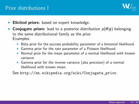
Prior distributions I

I Elicited priors: based on expert knowledge.

I Conjugate priors: lead to a posterior distribution p(θ|y) belongingto the same distributional family as the prior.Examples:

I Beta prior for the success probability parameter of a binomial likelihood.I Gamma prior for the rate parameter of a Poisson likelihood.I Normal prior for the mean parameter of a normal likelihood with known

variance.I Gamma prior for the inverse variance (aka precision) of a normal

likelihood with known mean.

See http://en.wikipedia.org/wiki/Conjugate_prior.


http://en.wikipedia.org/wiki/Conjugate_prior

Prior distributions II

I Noninformative priors: do not favor any values of θ if no a-prioriinformation is available. E.g.:

I Uniform distribution:I suitable if the parameter space is discrete and finite.I leads to improper priors (i.e., does not integrate to one) for continuous

and infinite parameter space.I is not (always) invariant under reparameterization.

I Jeffrey’s prior: invariant under reparameterization.

π(θ) ∝ |I (θ)|1/2,

where I (θ) is the expected Fisher information matrix with

Iij(θ) = −Ey|θ

[∂2

∂θi∂θjlog f (y|θ)

].

I Exercise: Jeffrey’s prior for binomial experiment.


Bayesian inference I

I Point estimation:I posterior mode (aka generalized ML estimate)I posterior mean or medianI . . .

I Interval estimation:

Definition

A 100× (1− α)% credible set for θ is a subset C of Ω such that

1− α ≤ P(C |y) =

∫Cp(θ|y)dθ.

The probability that θ lies in C given the observed data y is at least(1− α).


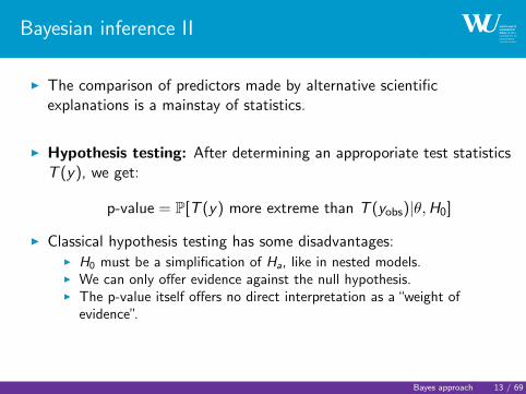
Bayesian inference II

I The comparison of predictors made by alternative scientificexplanations is a mainstay of statistics.

I Hypothesis testing: After determining an approporiate test statisticsT (y), we get:

p-value = P[T (y) more extreme than T (yobs)|θ,H0]

I Classical hypothesis testing has some disadvantages:I H0 must be a simplification of Ha, like in nested models.I We can only offer evidence against the null hypothesis.I The p-value itself offers no direct interpretation as a “weight of

evidence”.


Bayesian inference III

The Bayesian approach to hypothesis testing is much simpler:I As in the case for interval estimation, it requires some prior knowledge.I Based on the data that each of the hypotheses is supported to predict,

one applies Bayes’ Theorem and computes the posterior probabilitythat the first hypothesis is correct.


Bayesian inference IV

I Bayes factors:I The Bayes factor BF is the ratio of the posterior odds of model M1 to

the prior odds of M1:

BF =P(M1|y)/P(M2|y)

P(M1)/P(M2)

=p(y|M1)

p(y|M2),

i.e., the ratio of the observed marginal densities for the two models.I For two a priori equally probable models the BF equals the posterior

odds of M1. BF captures the change in the odds in favor of model 1 aswe move from prior to posterior.


Bayesian inference V

I Jeffrey’s scale for interpretation:

BF Strength of evidence< 1 Negative (support of M2)

1–3 Barely worth mentioning3–10 Substantial

10–30 Strong30–100 Very strong> 100 Decisive

I A fun reference: Wagenmakers, E.-J., Wetzels R., Borsboom D. andvan der Maas, H. (2011). Why Psychologists Must Change the WayThey Analyze Their Data: The Case of Psi. Journal of Personailtyand Social Psychology 100(3), 426–432.


Example: Consumer preference I

I 16 consumers have been recruited by a fast food chain to comparethe flavour of ground beef patties.

I The patties were kept frozen for eight months in different freezers:I a high-quality freezer consistenly maintaining the temperature at 0 F

(−18 C)I a freezer where the temperature varies between 0 and 15 F (−18 to−9 C).

I In a double-blind study (neither consumers nor waiters know wherethe patties were stored) each consumer evaluated patties from bothfridges.

I The food chain executives are interested in whether the higher-qualityfreezer leads to a substantial improvement in taste.

I The study result is that 13 out of 16 consumers prefer the moreexpensive patty.


Example: Consumer preference II

For a Bayesian analysis we need two components:I Likelihood:

I We assume that consumers are independent and that the probability θof preferring the more expensive patty is constant over the consumers.

I Their decisions form a sequence of Bernoulli trials.

Denoting the number of consumers preferring the more expensivepatty by Y gives

Y |θ ∼ Bin(16, θ),

which is equivalent to

f (y |θ) =

(16

y

)θy (1− θ)16−y .


Example: Consumer preference III

I Prior: The Beta distribution is a conjugate family for the binomialdistribution.

π(θ) =Γ(α + β)

Γ(α)Γ(β)θα−1(1− θ)β−1.

0.0 0.2 0.4 0.6 0.8 1.0

0.0

0.5

1.0

1.5

2.0

2.5

3.0

θ

prio

r de

nsity

Beta(.5, .5) (Jeffrey's prior)Beta(1, 1) (uniform prior)Beta(2, 2) (skeptical prior)


Example: Consumer preference IV

Thanks to the conjugacy the posterior distribution for θ is

p(θ|y) ∝ f (y |θ)π(θ) ∝ θy+α−1(1− θ)16−y+β−1

∝ Beta(y + α, 16− y + β)

0.0 0.2 0.4 0.6 0.8 1.0

01

23

4

θ

post

erio

r de

nsity

Beta(13.5, 3.5)Beta(14, 4)Beta(15, 5)


Example: Consumer preference V

I We return to the executives’ question concerning a substantialimprovement in taste.

I We select 0.6 as the critical value that θ must exceed in order for theimprovement to be regarded as “substantial”.

I Given this cutoff value, we compare the hypotheses M1 : θ ≥ 0.6 andM2 : θ < 0.6.

I Using a uniform prior we get for P(θ > .6|x):

> (p1 <- round(pbeta(0.6, 14, 4, lower.tail = FALSE),

+ digits = 3))

[1] 0.954


Example: Consumer preference VI

The Bayes factor is then given by

BF =0.954/0.046

0.4/0.6= 31.1.

This implies a reasonable strong preference for M1.


Bayesian computation

I Asymptotic methods

I Noniterative Monte Carlo methods

I Markov chain Monte Carlo methods

Bayesian computation 23 / 69

Development over time

I prehistory (1763–1960): Conjugate priors.

I 1960’s: Numerical quadrature (Newton-Cotes methods, Gaussianquadrature, etc.).

I 1970’s: Expectation-Maximization (EM) algorithm (iterative modefinder).

I 1980’s: Asymptotic methods.

I 1980’s: Noniterative Monte Carlo methods (direct posterior samplingand indirect methods, e.g., importance sampling, rejection).

I 1990’s: Markov chain Monte Carlo (MCMC; Gibbs sampling,Metropolis Hastings algorithm, etc.). ⇒ broadly applicable, butrequire care in parametrization and convergence diagnosis!

I 2000’s: Sequential Monte Carlo (SMC)


Normal approximation

When n is large, f (y |θ) will be quite peaked relative to π(θ), and sop(θ|y) will be approximately normal.Theorem (Bayesian Central Limit Theorem)

Suppose Y1, . . . ,Yniid∼ fi (yi |θ) and that the prior π(θ) and the likelihood

f (y|θ) are positive and twice differentiable near θπ, the posterior mode ofθ.Then for large n

p(θ|y).∼ N(θπ, [Iπ(y)]−1),

where [Iπ(y)]−1 is the “generalized” observed Fisher information matrix forθ, i.e., minus the inverse Hessian of the log posterior evaluated at themode.


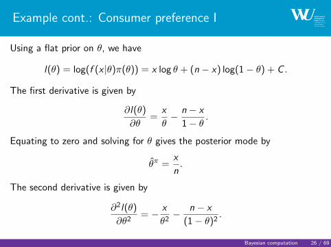
Example cont.: Consumer preference I

Using a flat prior on θ, we have

l(θ) = log(f (x |θ)π(θ)) = x log θ + (n − x) log(1− θ) + C .

The first derivative is given by

∂l(θ)

∂θ=

x

θ− n − x

1− θ.

Equating to zero and solving for θ gives the posterior mode by

θπ =x

n.

The second derivative is given by

∂2l(θ)

∂θ2= − x

θ2− n − x

(1− θ)2.


Example cont.: Consumer preference II

Evaluating at the estimate θπ gives

∂2l(θ)

∂θ2

∣∣∣∣θ=θπ

= − n

θπ(1− θπ).

Thus the posterior can be approximated by

p(θ|x).∼ N(θπ,

θπ(1− θπ)

n).


Example cont.: Consumer preference III

0.0 0.2 0.4 0.6 0.8 1.0

01

23

4

θ

post

erio

r de

nsity

exact (beta)approximate (normal)

Similar modes, but very different tail behavior.


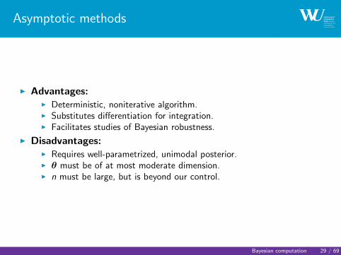
Asymptotic methods

I Advantages:I Deterministic, noniterative algorithm.I Substitutes differentiation for integration.I Facilitates studies of Bayesian robustness.

I Disadvantages:I Requires well-parametrized, unimodal posterior.I θ must be of at most moderate dimension.I n must be large, but is beyond our control.


Noniterative Monte Carlo methods

I Direct samplingI Indirect methods

I Importance samplingI Rejection sampling


Direct sampling

We begin with the most basic definition of Monte Carlo integration:

I Suppose θ ∼ p(θ) and we seek γ := E[c(θ)] =∫c(θ)p(θ)dθ.

I Then if θ1, . . . , θNiid∼ p(θ), we have

γ =1

N

N∑j=1

c(θj),

which converges to E[c(θ)] with probability 1 as N →∞.

I Hence the computation of posterior expectations requires only asample size of N from the posterior.


Importance sampling I

I Suppose we wish to approximate

E[h(θ)|y] =

∫h(θ)f (y|θ)π(θ)dθ∫f (y|θ)π(θ)dθ

.

Suppose further we can roughly approximate the normalized likelihoodtimes prior, cf (y|θ)π(θ), by some density g(θ) from which we caneasily sample.

I Then defining the weight function w(θ) = f (y|θ)π(θ)/g(θ),

E[h(θ)|y] =

∫h(θ)w(θ)g(θ)dθ∫w(θ)g(θ)dθ

≈1N

∑Nj=1 h(θj)w(θj)

1N

∑Nj=1 w(θj)

,

where θjiid∼ g(θ).

I Here, g(θ) is called the importance function; a good match tocf (y|θ)π(θ) will produce roughly equal weights.


Rejection sampling I

I Instead of trying to approximate the posterior

p(θ|y) =f (y|θ)π(θ)∫f (y|θ)π(θ)dθ

,

we try to find a majorizing function.

I Suppose there exists a constant M > 0 and a smooth density g(θ),called the envelope function, such that f (y|θ)π(θ) < Mg(θ) for all θ.

I The algorithm proceeds as follows:

(i) Generate θj ∼ g(θ).(ii) Generate U ∼ Unif(0, 1).(iii) If MUg(θj) < f (y|θj)π(θj), accept θj . Otherwise reject θj .(iv) Return to step (i) and repeat, until the desired sample size is obtained.

I The final sample consists of random draws from p(θ|y).


Rejection sampling II

−3 −2 −1 0 1 2 3

0.0

0.1

0.2

0.3

0.4

0.5

0.6

a

Lp

Mg

I Consider the θj samples in the histogram bar centered at a: therejection step “slices off” the top portion of the bar.

I Repeat for all a: accepted θjs mimic the lower curve!

I Need to choose M as small as possible (efficiency), and watch for“envelope violations”!


Markov chain Monte Carlo methods I

I Iterative MC methods are useful when it is difficult or impossible tofind a feasible importance or envelope density.

I Algorithms:I Gibbs samplerI Metropolis-Hastings algorithmI Slice sampler

I Performance evaluation:I Convergence monitoring and diagnosticsI Variance estimation


Markov chain Monte Carlo methods II

I Given two unknowns x and y , we can often write

p(x) =

∫p(x |y)p(y)dy and p(y) =

∫p(y |x)p(x)dx ,

where p(x |y) and p(y |x) are known.

I Seeking p(x) the analytical solution via substitution is:

p(x) =

∫p(x |y)

∫p(y |x ′)p(x ′)dx ′dy =

∫h(x , x ′)p(x ′)dx ′,

where h(x , x ′) =∫p(x |y)p(y |x ′)dy .

I This determines a fixed point system which converges under mildconditions.

pi+1(x) =

∫h(x , x ′)pi (x

′)dx ′


Markov chain Monte Carlo methods III

I Tanner and Wong (1987) showed that one can also use asampling-based approach which they refer to as data augmentation.

1. Draw X (0) ∼ p0(x).2. Draw Y (1) ∼ p(y |x (0)).3. Finally, X (1) ∼ p(x |y (1)).

I Then X (1) has marginal distribution

p1(x) =

∫p(x |y)p1(y)dy =

∫h(x , x ′)p0(x ′)dx ′.

I Repeating this process produces pairs (X (i),Y (i)) such that

X (i) d→ X ∼ p(x) and Y (i) d→ Y ∼ p(y).

I The luxury of avoiding the integration above has come at the price ofobtaining not the marginal density p(x) itself, but only a samplefrom this density.


Gibbs sampling I

I Suppose the joint distribution of θ = (θ1, . . . , θK ) is uniquelydetermined by the full conditional distributions,pi (θi |θj 6=i ), i = 1, . . . ,K.

I Given an arbitrary set of starting values θ(0)1 , . . . , θ(0)K ,

Draw θ(1)1 ∼ p1(θ1|θ(0)2 , . . . , θ

(0)K ),

Draw θ(1)2 ∼ p2(θ2|θ(1)1 , θ

(0)2 , . . . , θ

(0)K ),

...

Draw θ(1)K ∼ pK (θK |θ

(1)1 , . . . , θ

(1)K−1).

I Under mild conditions,

(θ(t)1 , . . . , θ

(t)K )

d→ (θ1, . . . , θK ) ∼ p as t →∞.


Gibbs sampling II

I For T sufficiently large (say, bigger than t0), θ(t)Tt=t0+1 is a(correlated) sample from the true posterior.

I We might use a sample mean to estimate the posterior mean

E(θi |y) ≈ 1

T − to

T∑t=t0+1

θ(t)i .

I The time from t = 0 to t = t0 is commonly known as the burn-inperiod.

I We may also run m parallel Gibbs sampling chains and obtain

E(θi |y) ≈ 1

m(T − to)

m∑j=1

T∑t=t0+1

θ(j ,t)i ,

where the index j indicates chain number.


Metropolis algorithm I

I What happens if the full conditional p(θi |θj 6=i , y) is not available inclosed form?

I Typically, p(θi |θj 6=i , y) will be available up to a proportionalityconstant, since it is proportional to the part of the Bayesian model(likelihood times prior) that involves θi .

I Suppose the true joint posterior for θ has unnormalized density p(θ).

I Choose a candidate density q(θ∗|θ(t−1)) that is a valid densityfunction for every possible value of the conditioning variable θ(t−1),and satisfies

q(θ∗|θ(t−1)) = q(θ(t−1)|θ∗),

i.e., q is symmetric in its arguments.


Metropolis algorithm II

I Given a starting value θ(0) at iteration t = 0, the algorithm proceedsas follows.For t = 1, . . . ,T repeat:

1. Draw θ∗ from q(·|θ(t−1)).2. Compute the ratio

r =p(θ∗)

p(θ(t−1)).

3. If r ≥ 1, set θ(t) = θ∗;

If r < 1, set θ(t) =

θ∗ with probability rθ(t−1) with probability 1− r

.

I Then a draw θ(t) converges in distribution to a draw from the trueposterior density p(θ|y).

I Note: When used as a substep in a larger (e.g., Gibbs) algorithm, weoften use T = 1 (convergence still OK).


Metropolis algorithm III

I How to choose the candidate density?

I The usual approach (after θ has been transformed to have supportRK , if necessary) is to set

q(θ∗|θ(t−1)) = N(θ∗|θ(t−1), Σ).

In one dimension Σ is often chosen to provide an observed acceptanceratio near 50%:

I Very small steps ⇒ High acceptance rate, but also highauto-correlation.

I Very large steps ⇒ Low acceptance rate and also high auto-correlation.


Metropolis algorithm IV

I Metropolis-Hastings algorithm:Hastings (1970) showed we can drop the requirement that q besymmetric, provided we use

r =p(θ∗)q(θ(t−1)|θ∗)

p(θ(t−1))q(θ∗|θ(t−1)).

This is useful for asymmetric target densities.


Auxiliary variables: Simple slice sampler I

I Ease and/or accelerate sampling from p(θ) by adding an auxiliary (orlatent) variable U ∼ p(u|θ).

I Suppose we want to sample a univariate θ from p(θ|y) ∝ h(θ). Weadd an auxiliary variable U such that U|θ ∼ Unif(0, h(θ)). The thejoint distribution of θ and U is

p(θ, u) ∝ h(θ)1

h(θ)I (u < h(θ)) = I (u < h(θ)),

where I denotes the indicator function.I The Gibbs sampler for this joint distribution is given by

1. u|θ ∼ Unif(0, p(θ)), and2. θ|u ∼ Unif(θ : p(θ) ≥ u).

I The second update (over the “slice” defined by u) requires p(θ) to beinvertible, either analytically or numerically.


Convergence assessment

When is it safe to stop and summarize MCMC output?

I We would like to ensure that∫|pt(θ)− p(θ)|dθ < ε.

But all we can hope to see is∫|pt(θ)− pt+k(θ)|dθ < ε.

I One can never “prove” convergence of a MCMC algorithm using onlya finite realization from the chain.

I A slowly converging sampler may be indistinguishable from one thatwill never converge (e.g., due to nonidentifiability)!

I Does the eventual mixing of “initially overdispersed” parallel samplingchains provide worthwhile information on convergence?

I Poor mixing of parallel chains can help discover extreme forms ofnonconvergence.


Convergence diagnostics

Various summaries of MCMC output, such asI Sample auto-correlations in one or more chains:

I Close to 0 indicates near-independence → Chain should quicklytraverse the entire parameter space.

I Close to 1 indicates that the sampler is “stuck”.

I Diagnostic tests requiring several chains include for example Gelman& Rubin’s shrink factor.

I Other tests for convergence requiring only one chain include amongothers Heidelberger & Welch’s, Raftery & Lewis’s and Geweke’sdiagnostics.


(Possible) Convergence diagnostics strategy

I Run a few (3 to 5) parallel chains, with starting points believed to beoverdispersed.

I E.g., covering ±3 prior standard deviations from the prior mean.

I Overlay the resulting sample traces for the parameters or arepresentative subset (if there are many parameters or a hierarchicalmodel is fitted).

I Annotate each plot with lag 1 sample autocorrelations and perhapsGelman & Rubin’s diagnostics.

I Look at convergence diagnostic tests output.

I Investigate bivariate plots and crosscorrelations among parameterssuspected of being confounded, just as one might do regardingcollinearity in linear regression.


Variance estimation I

How good is our MCMC estimate once we get it?

I Suppose we have a single long chain of (post-convergence) MCMCsamples θ(t)Tt=1. Let

θT = E[θ|y] =1

T

T∑t=1

θ(t).

I Then by the CLT, under iid sampling we could take

Viid[θT ] =s2θT

=1

T (T − 1)

T∑t=1

(θ(t) − θT )2.

But this is likely an underestimate due to positive autocorrelation inthe MCMC samples.


Variance estimation II

I To avoid wasteful parallel sampling or “thinning”, compute theeffective sample size,

ESS =T

κ(θ),

where κ(θ) = 1 + 2∑∞

k=1 ρk(θ) is the autocorrelation time, and wecut off the sum when ρk(θ) < ε.Then

VESS(θT ) =s2θ

ESS(θ).

Note: κ(θ) ≥ 1, so ESS(θ) ≤ T , and so we have that VESS ≥ Viid asexpected.


Variance estimation III

I Another alternative: BatchingDivide the run into m successive batches of length k with batchmeans b1, . . . , bm. Then θT = b = 1

m

∑mi=1 bi , and

Vbatch(θT ) =1

m(m − 1)

m∑i=1

(bi − θT )2,

provided that k is large enough so that the correlation betweenbatches is negligible.

I For any V used to approximate V(θN), a 95% CI for E[θ|y] is thengiven by

θT ± z0.025

√V.


Hands-on example: Bayesian Linear Model

I Observation equation: y|β, σ2 ∼ N(Xβ, σ2I

)

I Prior distributions: β|σ2 ∼ N(b0, σ

2B0

), σ2 ∼ G−1 (c0,C0)

According to Bayes formula, the posterior density is given through

p(β, σ2|y) ∝ p(y|β, σ2)︸︷︷︸likelihood

p(β, σ2)︸︷︷︸prior

= p(y|β, σ2)p(β|σ2)p(σ2)

∝(

1

σ

)n

exp

− 1

2σ2(y − Xβ)′(y − Xβ)

×(

1

σ

)p

exp

− 1

2σ2(β − b0)′B−10 (β − b0)

×(

1

σ2

)c0+1

exp

−C0

σ2

A hands-on example: Linear Model 51 / 69

Hands-on example: Bayesian Linear Model

I Observation equation: y|β, σ2 ∼ N(Xβ, σ2I

)I Prior distributions: β|σ2 ∼ N

(b0, σ

2B0

), σ2 ∼ G−1 (c0,C0)

According to Bayes formula, the posterior density is given through

p(β, σ2|y) ∝ p(y|β, σ2)︸︷︷︸likelihood

p(β, σ2)︸︷︷︸prior

= p(y|β, σ2)p(β|σ2)p(σ2)

∝(

1

σ

)n

exp

− 1

2σ2(y − Xβ)′(y − Xβ)

×(

1

σ

)p

exp

− 1

2σ2(β − b0)′B−10 (β − b0)

×(

1

σ2

)c0+1

exp

−C0

σ2


Bayesian Linear Model II: A Solution

The posterior β, σ2|y follows a so-called “normal-inverse-gamma”distribution, for which it can be shown that

βBayes := E[β|y] = (X′X + B−10 )−1(B−10 b0 + X′y)

Setting A = (X′X + B−10 )−1X′X, we can interpret βBayes as the weighted

mean of prior expectation b0 and OLS estimate βOLS:

βBayes = (I− A)b0 + AβOLS

Note that when the diagonal elements of B0 are large, A approaches I andthus βBayes approaches βOLS. Vice versa, when B0 has small diagonal

elements, A approaches 0, thus βBayes approaches b0.


Bayesian Linear Model III: Another Solution

What to do if you don’t speak normal-inverse-gamma-ish, or you want tofind a more flexible way of learning about the posterior distribution?

⇓

Use the Gibbs-sampler to “surf the posterior” by alternately simulatingvalues from the (full) conditional parameter densities β|y, σ2 and σ2|y,β.


Bayesian Linear Model IV: Hands On!

I β|y, σ2 ∼ N (bn,Bn) with

Bn =

(1

σ2X′X +

1

σ2B−10

)−1bn = Bn

(1

σ2X′y +

1

σ2B−10 b0

)

I σ2|y,β ∼ G−1 (cn,Cn) with

cn = c0 +n

2+

p

2

Cn = C0 +1

2(y − Xβ)′(y − Xβ) +

1

2(β − b0)′B−10 (β − b0)


Available tools for estimation

I General purpose estimation tools are provided by the BUGS family:

1. WinBUGS2. OpenBUGS3. JAGS

I Models are specified via variants of the BUGS language.I The software parses the model and determines the samplers

automatically to generate draws from the posterior.

Available tools in R 55 / 69

Available tools in R

I Estimation:I R2WinBUGS allows to run WinBUGS & OpenBUGS from R.I rjags provides an interface to the JAGS library.

I Post-processing, convergence diagnostics:I coda (Convergence Diagnosis and Output Analysis):

I contains a suite of functions that can be used to summarize, plot, andand diagnose convergence from MCMC samples.

I can easily import MCMC output from WinBUGS, OpenBUGS, andJAGS, or from plain matrices.

I provides the Gelman & Rubin, Geweke, Heidelberger & Welch, andRaftery & Lewis diagnostics.

For more information see the CRAN Task View: Bayesian Inference.

Available tools in R 56 / 69

Data I

I The data consists of a time series of daily Pound/Dollar exchange rates xtfrom 01/10/81 to 28/06/85. We have this data available in package Ecdatin R.

> data("Garch", package = "Ecdat")

> Garch <- subset(Garch,

+ date >= 811001 & date <= 850628,

+ c(date, bp))

> x <- Garch$bp

I The series of interest are the daily mean-corrected returns times hundred,yt for t = 1, . . . , n.

yt = 100

[log xt − log xt−1 −

1

n

n∑i=1

(log xt − log xt−1)

],

> y <- 100 * diff(log(x))

> y <- y - mean(y)

Example: Stochastic volatility models 57 / 69

Data II

Date

y

−2

01

23

4

1982 1983 1984 1985

01

23

Date

abs(

y)


Model I

I The stochastic volatility model can be written in the form of anonlinear state-space model.

I A state-space model specifices the conditional distributions of theobservations given unkown states, here the underlying latentvolatilities, θt , in the observation equations for t = 1, . . . , n

yt |θt = exp

(1

2θt

)ut , ut

iid∼ N(0, 1).

I The unkown states are assumed to follow a Markovian transition overtime given by the state equations for t = 1, . . . , n

θt |θt−1, µ, φ, τ2 = µ+ φ(θt−1 − µ) + νt , νtiid∼ N(0, τ2).

with θ0 ∼ N(µ, τ2).


Model II

I The state θt determines the amount of volatility on day t.

I φ measures the autocorrelation present in the logged squared dataand is restricted to be −1 < φ < 1. It can be interpreted as thepersistence in the volatility.

I The constant scaling factor β = exp(µ/2) can be seen as the modalvolatility.

I τ2 is the volatility of log-volatilities.

I Remark: For Bayesian estimation the parameterization of the normaldistribution is in general with respect to mean µ and precision τ , i.e.,

y ∼ dnorm(µ, τ),

where τ = σ−2, i.e., the precision is the inverse of the variance. Theconjugate prior for the precision is the Gamma distribution.


Model III

The full Bayesian model consists of

I a prior for the unobservablesI 3 parameters: µ, φ, τ 2

I unkown states: θ0, . . . , θn

p(µ, φ, τ2, θ0, . . . , θn) = p(µ, φ, τ2)p(θ0|µ, τ2)n∏

t=1

p(θt |θt−1, µ, φ, τ2),

I a joint distribution for the observables y1, . . . , yn

p(y1, . . . , yn|µ, φ, τ2, θ0, . . . , θn) =n∏

t=1

p(yt |θt).


Model specification in BUGS I

model

for (t in 1:length(y))

y[t] ~ dnorm(0, 1/exp(theta[t]));

theta0 ~ dnorm(mu, itau2);

theta[1] ~ dnorm(mu + phi * (theta0 - mu), itau2);

for (t in 2:length(y))

theta[t] ~ dnorm(mu + phi * (theta[t-1] - mu), itau2);

## prior

mu ~ dnorm(0, 0.1);

phistar ~ dbeta(20, 1.5);

itau2 ~ dgamma(2.5, 0.025);

## transform

beta <- exp(mu/2);

tau <- sqrt(1/itau2);

phi <- 2 * phistar - 1


Estimation with JAGS I

I Given the model specification a graphical model is constructed todetermine the parents and direct children of each variable/node.

I Based on these relationships suitable samplers are selected (from thebase and bugs module):

I Conjugate sampler: for Gibbs sampling.I Finite sampler: discrete valued node with fixed support of less than

20 possible values, not bounded using truncation.I Discrete slice sampler: for any scalar discrete-valued stochastic node.I Real slice sampler: for any scalar real-valued stochastic node.


Estimation with JAGS II

> library("rjags")

> initials <-

+ list(list(phistar = 0.975, mu = 10, itau2 = 300),

+ list(phistar = 0.5, mu = 0, itau2 = 50),

+ list(phistar = 0.025, mu = -10, itau2 = 1))

> initials <- lapply(initials, "c",

+ list(.RNG.name = "base::Wichmann-Hill",

+ .RNG.seed = 2207))

> model <- jags.model("volatility.bug", data = list(y = y),

+ inits = initials, n.chains = 3)

> update(model, n.iter = 10000)

> draws <- coda.samples(model, c("phi", "tau", "beta"),

+ n.iter = 100000, thin = 20)

> summary(draws)


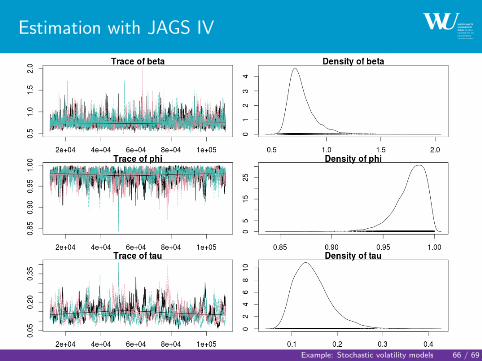
Estimation with JAGS III

Iterations = 11020:111000

Thinning interval = 20

Number of chains = 3

Sample size per chain = 5000

1. Empirical mean and standard deviation for each variable,

plus standard error of the mean:

Mean SD Naive SE Time-series SE

beta 0.770 0.1231 0.001005 0.003436

phi 0.977 0.0150 0.000122 0.000676

tau 0.145 0.0408 0.000333 0.002469

2. Quantiles for each variable:

2.5% 25% 50% 75% 97.5%

beta 0.611 0.689 0.744 0.821 1.084

phi 0.940 0.969 0.980 0.988 0.997

tau 0.085 0.116 0.139 0.167 0.243


Estimation with JAGS IV


Diagnostics with coda I

I Auto- and crosscorrelation: autocorr.diag, autocorr.plot,crosscorr

I Gelman and Rubin diagnostics: gelman.diag

I Heidelberger and Welch diagnostics: heidel.diag

I Geweke diagnostics: geweke.diag, geweke.plot

I Raftery and Lewis diagnostics: raftery.diag

For more information see the CODA manual at http://www.mrc-bsu.cam.ac.uk/bugs/documentation/Download/cdaman03.pdf and theaddendum to the manual at http://www.mrc-bsu.cam.ac.uk/bugs/documentation/Download/cdaman04.pdf


http://www.mrc-bsu.cam.ac.uk/bugs/documentation/Download/cdaman03.pdf




Literature I

Albert, J. (2007) Bayesian Computation with R. Springer.

Carlin, B. P. (2010) Introduction to Bayesian Analysis. Course materialavailable at http://www.biostat.umn.edu/~brad.

Carlin, B. P. and Louis, T. A. (2009) Bayesian Methods for Data Analysis.3rd, CRC Press.

Cowles, M. K. and Carlin, B. P. (1996) Markov chain Monte Carloconvergence diagnostics: a comparative review. Journal of the AmericanStatistical Association 91(434), 883–904.

Chib, S., Griffiths W. and Koop G. (2008) Bayesian Econometrics. EmeralGroup Publishing Ltd.

Hastings, W. K. (1970) Monte Carlo sampling methods using Markovchains and their applications. Biometrika 57, 97–109.

Literature 68 / 69

http://www.biostat.umn.edu/~brad

Literature II

Neal, R. M. (2003) Slice sampling. Annals of Statistics 31(3), 705–741.

Meyer, R. and Yu J. (2000) BUGS for a Bayesian analysis of stochasticvolatility models. Econometrics Journal 3, 198–215.

Tanner, M. A. and Wong, W. H. (1987) The Calculation of PosteriorDistributions by Data Augmentation. Journal of the American StatisticalAssociation, 82(398): 528–540.

Watsham, T. J. and Parramore, K. (1997) Quantitative Methods inFinance. Cengage Learning EMEA.

Literature 69 / 69

bayesian computation with r - institute for statistics and...

Documents