26/04/16

1

Bayesian Belief Network

n  Uncertainty & Probabilityn  Baye's rulen  Choosing Hypotheses- Maximum a posteriori n  Maximum Likelihood - Baye's concept learningn  Maximum Likelihood of real valued functionn  Bayes optimal Classifiern  Joint distributionsn  Naive Bayes Classifier

26/04/16

2

Uncertaintyn Our main tool is the probability theory, which

assigns to each sentence numerical degree of belief between 0 and 1

n  It provides a way of summarizing the uncertainty

Variablesn  Boolean random variables: cavity might be true or false n  Discrete random variables: weather might be sunny, rainy,

cloudy, snown  P(Weather=sunny)n  P(Weather=rainy)n  P(Weather=cloudy)n  P(Weather=snow)

n  Continuous random variables: the temperature has continuous values

26/04/16

3

Where do probabilities come from?n  Frequents:

n  From experiments: form any finite sample, we can estimate the true fraction and also calculate how accurate our estimation is likely to be

n  Subjective:n  Agent’s believe

n  Objectivist:n  True nature of the universe, that the probability up heads with

probability 0.5 is a probability of the coin

n  Before the evidence is obtained; prior probabilityn  P(a) the prior probability that the proposition is truen  P(cavity)=0.1

n  After the evidence is obtained; posterior probability n  P(a|b) n  The probability of a given that all we know is bn  P(cavity|toothache)=0.8

26/04/16

4

Axioms of Probability (Kolmogorov’s axioms, first published in German 1933)

n  All probabilities are between 0 and 1. For any proposition a 0 ≤ P(a) ≤ 1

n  P(true)=1, P(false)=0 n  The probability of disjunction is given by�

€

P(a∨b) = P(a) + P(b) − P(a∧b)

n Product rule

)()|()()()|()(aPabPbaPbPbaPbaP

=∧

=∧

26/04/16

5

Theorem of total probabilityIf events A1, ... , An are mutually

exclusive with then

Bayes’s rule n  (Reverent Thomas Bayes 1702-1761)

•  He set down his findings on probability in "Essay Towards Solving a Problem in the Doctrine of Chances" (1763), published posthumously in the Philosophical Transactions of the Royal Society of London

€

P(b | a) =P(a |b)P(b)

P(a)

26/04/16

6

Diagnosisn  What is the probability of meningitis in the patient with stiff

neck?

n  A doctor knows that the disease meningitis causes the patient to have a stiff neck in 50% of the time -> P(s|m)

n  Prior Probabilities: •  That the patient has meningitis is 1/50.000 -> P(m)•  That the patient has a stiff neck is 1/20 -> P(s)

€

P(m | s) =0.5*0.00002

0.05= 0.0002

€

P(m | s) =P(s |m)P(m)

P(s)

Normalization

)()()|()|(

)()()|()|(

xPyPyxP

xyP

xPyPyxP

xyP

¬¬=¬

=

4.0,6.008.0,12.0

)|(),|(

)()|()|(

)|()|(1

=

¬

×=

¬+=

α

α

α

xyPxyP

YPYXPXYP

xyPxyP

26/04/16

7

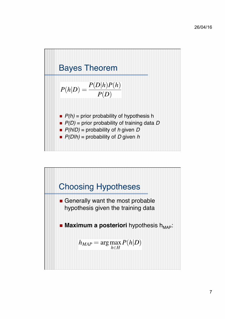
Bayes Theorem

n  P(h) = prior probability of hypothesis hn  P(D) = prior probability of training data Dn  P(h|D) = probability of h given Dn  P(D|h) = probability of D given h

Choosing Hypothesesn Generally want the most probable

hypothesis given the training data

n Maximum a posteriori hypothesis hMAP:

26/04/16

8

n  If assume P(hi)=P(hj) for all hi and hj, then can further simplify, and choose the

n Maximum likelihood (ML) hypothesis

26/04/16

9

Examplen  Does patient have cancer or not?

A patient takes a lab test and the result comes back positive. The test returns a correct positive result (+) in only 98% of the cases in which the disease is actually present, and a correct negative result (-) in only 97% of the cases in which the disease is not present

Furthermore, 0.008 of the entire population have this cancer

Suppose a positive result (+) is returned...

26/04/16

10

Normalization

n The result of Bayesian inference depends strongly on the prior probabilities, which must be available in order to apply the method

€

P(cancer |+) =0.0078

0.0078 + 0.0298= 0.20745

€

P(¬cancer | +) =0.0298

0.0078 + 0.0298= 0.79255

Joint distribution

n  A joint distribution for toothache, cavity, catch, dentist‘s probe catches in my tooth :-(

n  We need to know the conditional probabilities of the conjunction of toothache and cavity

n  What can a dentist conclude if the probe catches in the aching tooth?

n  For n possible variables there are 2n possible combinations€

P(cavity | toothache∧catch) =P(toothache∧catch | cavity)P(cavity)

P(toothache∧cavity)

26/04/16

11

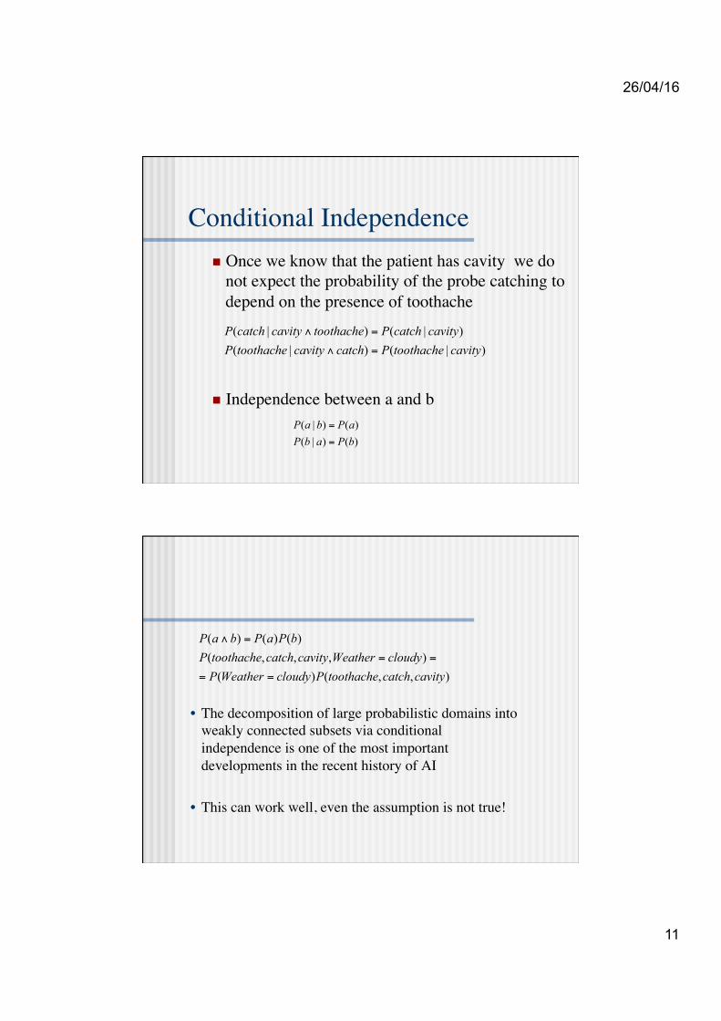
Conditional Independencen  Once we know that the patient has cavity we do

not expect the probability of the probe catching to depend on the presence of toothache

n  Independence between a and b

)|()|()|()|(cavitytoothachePcatchcavitytoothacheP

cavitycatchPtoothachecavitycatchP=∧

=∧

)()|()()|(bPabPaPbaP

=

=

•  The decomposition of large probabilistic domains into weakly connected subsets via conditional independence is one of the most important developments in the recent history of AI

•  This can work well, even the assumption is not true!

),,()(),,,(

)()()(

cavitycatchtoothachePcloudyWeatherPcloudyWeathercavitycatchtoothacheP

bPaPbaP

==

==

=∧

26/04/16

12

A single cause directly influence a number of effects, all of which are conditionally independent

)|()(),...,,(1

21 causeeffectPcausePeffecteffecteffectcausePn

iin ∏

=

=

Naive Bayes Classifiern Assume target function f: X è V, where

each instance x described by attributes a1, a2 .. an

n Most probable value of f(x) is:

26/04/16

13

vNB

n Naive Bayes assumption:

n which gives

Naive Bayes Algorithm n For each target value vjn  ç estimate P(vj)n For each attribute value ai of each

attribute an  ç estimate P(ai|vj)

26/04/16

14

Training datasetage income student credit_rating buys_computer

<=30 high no fair no<=30 high no excellent no30…40 high no fair yes>40 medium no fair yes>40 low yes fair yes>40 low yes excellent no31…40 low yes excellent yes<=30 medium no fair no<=30 low yes fair yes>40 medium yes fair yes<=30 medium yes excellent yes31…40 medium no excellent yes31…40 high yes fair yes>40 medium no excellent no

Class: C1:buys_computer=‘yes’ C2:buys_computer=‘no’ Data sample: X = (age<=30, Income=medium, Student=yes Credit_rating=Fair)

Naïve Bayesian Classifier: Example

n  Compute P(X|Ci) for each class

P(age=“<30” | buys_computer=“yes”) = 2/9=0.222 P(age=“<30” | buys_computer=“no”) = 3/5 =0.6 P(income=“medium” | buys_computer=“yes”)= 4/9 =0.444 P(income=“medium” | buys_computer=“no”) = 2/5 = 0.4 P(student=“yes” | buys_computer=“yes)= 6/9 =0.667 P(student=“yes” | buys_computer=“no”)= 1/5=0.2 P(credit_rating=“fair” | buys_computer=“yes”)=6/9=0.667 P(credit_rating=“fair” | buys_computer=“no”)=2/5=0.4

n  X=(age<=30 ,income =medium, student=yes,credit_rating=fair)

P(X|Ci) : P(X|buys_computer=“yes”)= 0.222 x 0.444 x 0.667 x 0.0.667 =0.044 P(X|buys_computer=“no”)= 0.6 x 0.4 x 0.2 x 0.4 =0.019

P(X|Ci)*P(Ci ) : P(X|buys_computer=“yes”) * P(buys_computer=“yes”)=0.028 P(X|buys_computer=“no”) * P(buys_computer=“no”)=0.007

§  X belongs to class “buys_computer=yes”

P(buys_computer=„yes“)=9/14

P(buys_computer=„no“)=5/14

26/04/16

15

n  Conditional independence assumption is often violated

n  ...but it works surprisingly well anyway

n  Naive Bayes assumption of conditional independence too restrictive

n  But it's intractable without some such assumptions...

n  Bayesian Belief networks describe conditional independence among subsets of variables

n  allows combining prior knowledge about (in)dependencies among variables with observed training data

26/04/16

16

Bayesian networksn  A simple, graphical notation for conditional independence

assertions and hence for compact specification of full joint distributions

n  Syntax:n  a set of nodes, one per variable

n  a directed, acyclic graph (link ≈ "directly influences")n  a conditional distribution for each node given its parents:

P (Xi | Parents (Xi))

n  In the simplest case, conditional distribution represented as a conditional probability table (CPT) giving the distribution over Xi for each combination of parent values

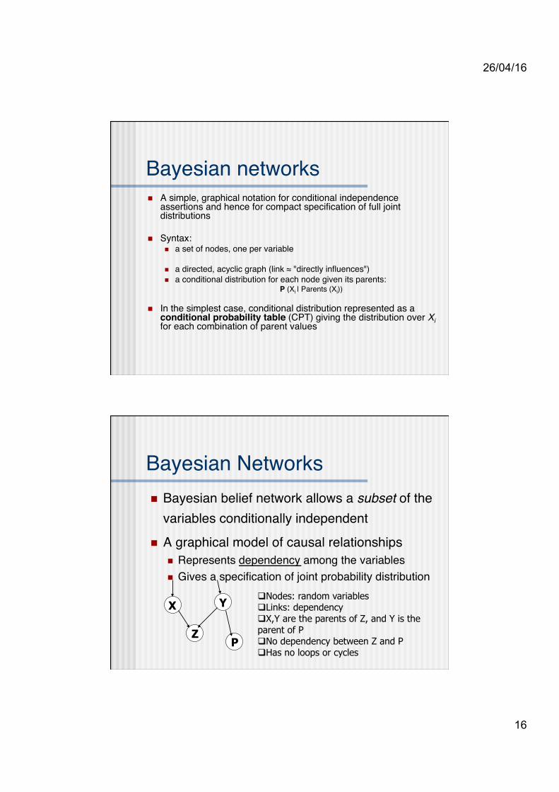
Bayesian Networksn  Bayesian belief network allows a subset of the

variables conditionally independent

n  A graphical model of causal relationshipsn  Represents dependency among the variables n  Gives a specification of joint probability distribution

X Y

Z P

q Nodes: random variables q Links: dependency q X,Y are the parents of Z, and Y is the parent of P q No dependency between Z and P q Has no loops or cycles

26/04/16

17

Conditional Independencen  Once we know that the patient has cavity we do

not expect the probability of the probe catching to depend on the presence of toothache

n  Independence between a and b

)|()|()|()|(cavitytoothachePcatchcavitytoothacheP

cavitycatchPtoothachecavitycatchP=∧

=∧

)()|()()|(bPabPaPbaP

=

=

Examplen  Topology of network encodes conditional independence assertions:

n  Weather is independent of the other variablesn  Toothache and Catch are conditionally independent given Cavity

26/04/16

18

Bayesian Belief Network: An Example

Family History

LungCancer

PositiveXRay

Smoker

Emphysema

Dyspnea

LC

~LC

(FH, S) (FH, ~S) (~FH, S) (~FH, ~S)

0.8

0.2

0.5

0.5

0.7

0.3

0.1

0.9

Bayesian Belief Networks

The conditional probability table for the variable LungCancer: Shows the conditional probability for each possible combination of its parents

Examplen  I'm at work, neighbor John calls to say my alarm is ringing, but neighbor

Mary doesn't call. Sometimes it's set off by minor earthquakes. Is there a burglar?

n  Variables: Burglary, Earthquake, Alarm, JohnCalls, MaryCalls

n  Network topology reflects "causal" knowledge:

n  A burglar can set the alarm offn  An earthquake can set the alarm offn  The alarm can cause Mary to calln  The alarm can cause John to call

26/04/16

19

Belief Networks

Burglary P(B) 0.001

Earthquake P(E) 0.002

Alarm Burg. Earth. P(A) t t .95 t f .94 f t .29 f f .001

JohnCalls MaryCalls A P(J) t .90 f .05

A P(M) t .7 f .01

Full Joint Distribution

))(|(),...,(1

1 i

n

iin XparentsxPxxP ∏

=

=

00062.0998.0999.0001.07.09.0)()()|()|()|(

)(

=××××=

¬¬¬∧¬=

¬∧¬∧∧∧

ePbPebaPamPajPebamjP

26/04/16

20

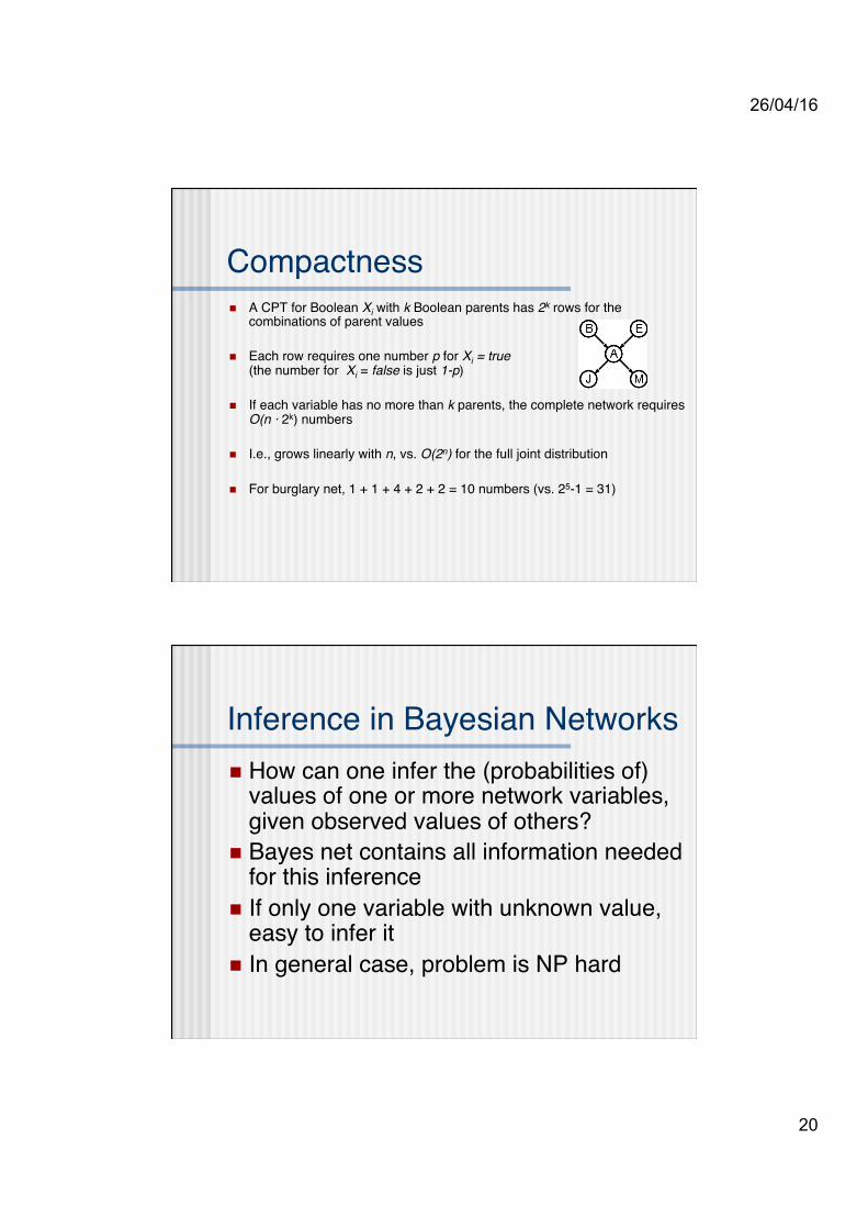
Compactnessn  A CPT for Boolean Xi with k Boolean parents has 2k rows for the

combinations of parent values

n  Each row requires one number p for Xi = true (the number for Xi = false is just 1-p)

n  If each variable has no more than k parents, the complete network requires O(n · 2k) numbers

n  I.e., grows linearly with n, vs. O(2n) for the full joint distribution

n  For burglary net, 1 + 1 + 4 + 2 + 2 = 10 numbers (vs. 25-1 = 31)

Inference in Bayesian Networksn How can one infer the (probabilities of)

values of one or more network variables, given observed values of others?

n Bayes net contains all information needed for this inference

n  If only one variable with unknown value, easy to infer it

n  In general case, problem is NP hard

26/04/16

21

Examplen  In the burglary network, we migth observe

the event in which JohnCalls=true and MarryCalls=true

n We could ask for the probability that the burglary has occurred

n  P(Burglary|JohnCalls=ture,MarryCalls=true)

Remember - Joint distribution

€

P(cavity | toothache) =P(cavity∧ toothache)

P(toothache)

€

P(¬cavity | toothache) =P(¬cavity∧ toothache)

P(toothache)€

=0.108 + 0.012

0.108 + 0.012 + 0.016 + 0.064= 0.6

€

=0.016 + 0.064

0.108 + 0.012 + 0.016 + 0.064= 0.4

26/04/16

22

Normalization

4.0,6.008.0,12.0

)|(),|(

)()|()|(

)|()|(1

=

¬

×=

¬+=

α

α

α

xyPxyP

YPYXPXYP

xyPxyP

Normalization

•  X is the query variable•  E evidence variable•  Y remaining unobservable variable

•  Summation over all possible y (all possible values of the unobservable variables Y)

€

P(Cavity | toothache) =αP(Cavity, toothache)=α[P(Cavity, toothache,catch) + P(Cavity, toothache,¬catch)]=α[< 0.108,0.016 > + < 0.012,0.064 >] =α < 0.12,0.08 >=< 0.6,0.4 >

€

P(X | e) =αP(X,e) =α P(X,e,y)y∑

26/04/16

23

n  P(Burglary|JohnCalls=ture,MarryCalls=true)•  The hidden variables of the query are Earthquake

and Alarm

•  For Burglary=true in the Bayesain network

€

P(B | j,m) =αP(B, j,m) =α P(B,e,a, j,m)a∑

e∑

€

P(b | j,m) =α P(b)P(e)P(a |b,e)P( j | a)P(m | a)a∑

e∑

n To compute we had to add four terms, each computed by multiplying five numbers

n  In the worst case, where we have to sum out almost all variables, the complexity of the network with n Boolean variables is O(n2n)

26/04/16

24

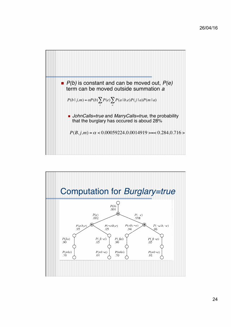
n  P(b) is constant and can be moved out, P(e) term can be moved outside summation a

n  JohnCalls=true and MarryCalls=true, the probability that the burglary has occured is aboud 28%€

P(b | j,m) =αP(b) P(e) P(a |b,e)P( j | a)P(m | a)a∑

e∑

€

P(B, j,m) =α < 0.00059224,0.0014919 >≈< 0.284,0.716 >

Computation for Burglary=true

26/04/16

25

Variable elimination algorithm•  Eliminate repeated calculation

•  Dynamic programming

Irrelevant variables•  (X query variable, E evidence variables)

26/04/16

26

Complexity of exact inference

n  The burglary network belongs to a family of networks in which there is at most one undirected path between tow nodes in the networkn  These are called singly connected networks or

polytreesn  The time and space complexity of exact

inference in polytrees is linear in the size of networkn  Size is defined by the number of CPT entriesn  If the number of parents of each node is bounded by

a constant, then the complexity will be also linear in the number of nodes

n For multiply connected networks variable elimination can have exponential time and space complexity

26/04/16

27

Constructing Bayesian Networksn A Bayesian network is a correct

representation of the domain only if each node is conditionally independent of its predecessors in the ordering, given its parents

P(MarryCalls|JohnCalls,Alarm,Eathquake,Bulgary)=P(MaryCalls|Alarm)

Conditional Independence relations in Bayesian networks

n The topological semantics is given either of the specifications of DESCENDANTS or MARKOV BLANKET

26/04/16

28

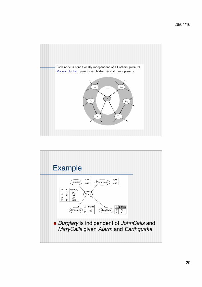
Local semantics

Example

n  JohnCalls is indipendent of Burglary and Earthquake given the value of Alarm

26/04/16

29

Example

n Burglary is indipendent of JohnCalls and MaryCalls given Alarm and Earthquake

26/04/16

30

Constructing Bayesian networksn  1. Choose an ordering of variables X1, … ,Xn

n  2. For i = 1 to nn  add Xi to the network

n  select parents from X1, … ,Xi-1 such thatP (Xi | Parents(Xi)) = P (Xi | X1, ... Xi-1)

This choice of parents guarantees:P (X1, … ,Xn) = πn

i =1 P (Xi | X1, … , Xi-1) (chain rule)

= πni =1P (Xi | Parents(Xi))

(by construction)

n  The compactness of Bayesian networks is an example of locally structured systemsn  Each subcomponent interacts directly with only

bounded number of other componentsn  Constructing Bayesian networks is difficult

n  Each variable should be directly influenced by only a few others

n  The network topology reflects thes direct influences

26/04/16

31

n  Suppose we choose the ordering M, J, A, B, E

P(J | M) = P(J)?

Example

n  Suppose we choose the ordering M, J, A, B, E

P(J | M) = P(J)?NoP(A | J, M) = P(A | J)? P(A | J, M) = P(A)? NoP(B | A, J, M) = P(B | A)? P(B | A, J, M) = P(B)?

Example

26/04/16

32

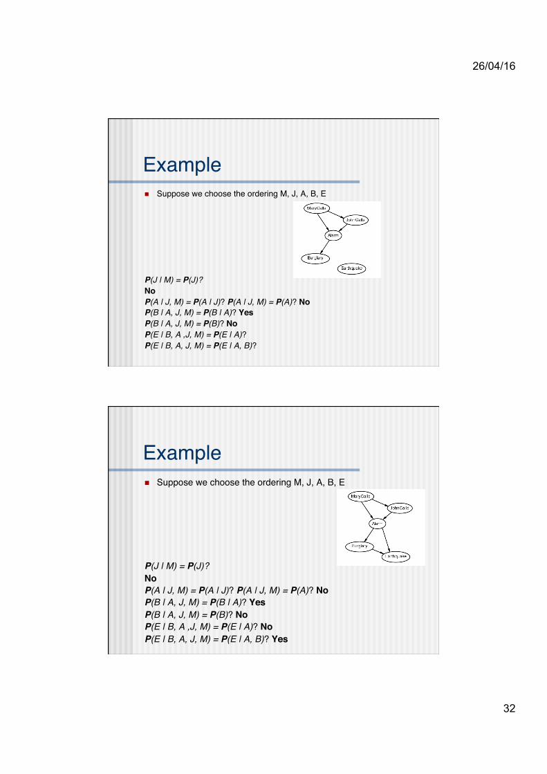
n  Suppose we choose the ordering M, J, A, B, E

P(J | M) = P(J)?NoP(A | J, M) = P(A | J)? P(A | J, M) = P(A)? NoP(B | A, J, M) = P(B | A)? YesP(B | A, J, M) = P(B)? NoP(E | B, A ,J, M) = P(E | A)?P(E | B, A, J, M) = P(E | A, B)?

Example

n  Suppose we choose the ordering M, J, A, B, E

P(J | M) = P(J)?No P(A | J, M) = P(A | J)? P(A | J, M) = P(A)? NoP(B | A, J, M) = P(B | A)? YesP(B | A, J, M) = P(B)? NoP(E | B, A ,J, M) = P(E | A)? NoP(E | B, A, J, M) = P(E | A, B)? Yes

Example

26/04/16

33

Example contd.

n  Deciding conditional independence is hard in no causal directions

n  (Causal models and conditional independence seem hardwired for humans!)

n  Network is less compact: 1 + 2 + 4 + 2 + 4 = 13 numbers neededn  Some links represent tenuous relationship that require difficult and unnatural

probability judgment, such the probability of Earthquake given Burglary and Alarm