bayesian analysis in mplus: a brief introduction 3.pdf · bayesian analysis in mplus: a brief...

Bayesian Analysis In Mplus:A Brief Introduction

Bengt MuthenIncomplete Draft, Version 3 ∗

May 17, 2010

∗I thank Tihomir Asparouhov and Linda Muthen for helpful comments

1

Abstract

This paper uses a series of examples to give an introduction to how Bayesian analysis

is carried out in Mplus. The examples are a mediation model with estimation of an

indirect effect, a structural equation model, a two-level regression model with estimation

of a random intercept variance, a multiple-indicator binary growth model with a large

number of latent variables, a two-part growth model, and a mixture model. It is shown

how the use of Mplus graphics provides information on estimates, convergence, and model

fit. Comparisons are made with frequentist estimation using maximum likelihood and

weighted least squares. Data and Mplus scripts are available on the Mplus website.

2

1 Introduction

Frequentist (e.g., maximum likelihood) and Bayesian analysis differ by the former viewing

parameters as constants and the latter as variables. Maximum likelihood (ML) finds

estimates by maximizing a likelihood computed for the data. Bayes combines prior

distributions for parameters with the data likelihood to form posterior distributions for

the parameter estimates. The priors can be diffuse (non-informative) or informative where

the information may come from previous studies. The posterior provides an estimate in

the form of a mean, median, or mode of the posterior distribution.

There are many books on Bayesian analysis and most are quite technical. Gelman

et al. (2004) provides a good general statistical description, whereas Lynch (2010)

gives a somewhat more introductory account. Lee (2007) gives a discussion from a

structural equation modeling perspective. Schafer (1997) gives a statistical discussion

from a missing data and multiple imputation perspective, whereas Enders (2010) gives an

applied discussion of these same topics. Statistical overview articles include Gelfand et al.

(1990) and Casella and George (1992). Overview articles of an applied nature and with

a latent variable focus include Scheines et al. (1999), Rupp et al. (2004), and Yuan and

MacKinnon (2009).

Bayesian analysis is firmly established in mainstream statistics. Its popularity is

growing and currently appears to be featured at least half as often as frequentist analysis.

Part of the reason for the increased use of Bayesian analysis is the success of new

computational algorithms referred to as Markov chain Monte Carlo (MCMC) methods.

Outside of statistics, however, application of Bayesian analysis lags behind. One possible

reason is that Bayesian analysis is perceived as difficult to do, requiring complex statistical

specifications such as those used in the flexible, but technically-oriented general Bayes

program WinBUGS. These observations were the background for developing Bayesian

analysis in Mplus (Muthen & Muthen, 1998-2010). In Mplus, simple analysis specifications

3

with convenient defaults allow easy access to a rich set of analysis possibilities. Diffuse

priors are used as the default with the possibility of specifying informative priors. A range

of graphics options are available to easily provide information on estimates, convergence,

and model fit.

Three key points motivate taking an interest in Bayesian analysis:

1. More can be learned about parameter estimates and model fit

2. Analyses can be made less computationally demanding

3. New types of models can be analyzed

Point 1 is illustrated by parameter estimates that do not have a normal distribution.

ML gives a parameter estimate and its standard error and assumes that the distribution of

the parameter estimate is normal based on asymptotic (large-sample) theory. In contrast,

Bayes does not rely on large-sample theory and provides the whole distribution not

assuming that it is normal. The ML confidence interval Estimate± 1.96× SE assumes a

symmetric distribution, whereas the Bayesian credibility interval based on the percentiles

of the posterior allows for a strongly skewed distribution. Bayesian exploration of model fit

can be done in a flexible way using Posterior predictive checking (PPC; see, e.g., Gelman

et al., 1996; Gelman et al., 2004, Chapter 6; Lee, 2007, Chapter 5; Scheines et al., 1999).

Any suitable test statistics for the observed data can be compared to statistics based on

simulated data obtained via draws of parameter values from the posterior distribution,

avoiding statistical assumptions about the distribution of the test statistics. Examples

of non-normal posteriors are presented in Section 2 for single-level models as well as in

Section 4 for multilevel models. Examples of PPC are given in Section 3.

Point 2 may be of interest for an analyst who is hesitant to move from ML estimation

to Bayesian estimation. Many models are computationally cumbersome or impossible

using ML, such as with categorical outcomes and many latent variables resulting in many

dimensions of numerical integration. Such an analyst may view the Bayesian analysis

4

simply as a computational tool for getting estimates that are analogous to what would

have been obtained by ML had it been feasible. This is obtained with diffuse priors, in

which case ML and Bayesian results are expected to be close in large samples (Browne &

Draper, 2006; p. 505). Examples of this are presented in Section 5.

Point 3 is exemplified by models with a very large number of parameters or where ML

does not provide a natural approach. Examples of the former include image analysis (see,

e.g., Green, 1996)) and examples of the latter include random change-point analysis (see,

e.g., Dominicus et al., 2008).

This paper gives a brief introduction to Bayesian analysis as implemented in Mplus.

For a technical discussion of this implementation, see Asparouhov and Muthen (2010a)

with latent variable model investigations in Asparouhov and Muthen (2010b). Section 2

provides two mediation modeling examples which illustrate a non-normal posterior, how to

use priors, and how to do a basic Bayes analysis in Mplus. Section 3 uses a CFA example

to illustrate both informative priors and the use of PPC. Section 4 uses two-level regression

to illustrate how to get correct a correct assessment of the size of a skewed random effect

variance estimate and intraclass correlation even with a small number of clusters. Section

5 uses a two-part growth model to illustrate the speed advantage of Bayes over ML with

many dimensions. Section 6 uses multiple-indicator growth for binary items to illustrate

high-dimensional analysis that is not possible with ML. Section 7 uses a mixture model

to illustrate how to handle label switching. Section 8 discusses alternative approaches to

missing data modeling. Data and Mplus scripts are available on the Mplus web site under

Mplus Examples, Applications using Mplus.

5

2 Two mediation modeling examples

Two mediation modeling examples are considered. The first example uses the ATLAS data

of MacKinnon et al. (2004) and illustrates how different conclusions about the intervention

effect are arrived at using ML versus Bayes. The second example uses the firefighter data

of Yuan and MacKinnon (2009) to illustrate the use of priors based on information from

previous studies to shorten the credibility interval (the Bayesian counterpart to confidence

intervals) for the intervention effect.

2.1 The ATLAS example: Different conclusions using Bayes

vs ML

The mediational model in Figure 1 was considered in MacKinnon et al. (2004). The

intervention program ATLAS (Adolescent Training and Learning to Avoid Steroids) was

administered to high school football players to prevent use of anabolic steroids. MacKinnon

et al. (2004) used a sample of n = 861 with complete data from 15 treatment schools and

16 control schools (the multilevel nature of the data was ignored and is ignored here as

well; multilevel Bayesian mediational modeling is, however, available in Mplus). One part

of the intervention aimed at increasing perceived severity of using steroids. This in turn

was hypothesized to increase good nutrition behaviors. In Figure 1 these three variables

are denoted tx, severity, and nutrition, respectively.

[Figure 1 about here.]

A key parameter is the indirect effect of intervention on the nutrition outcome, a× b.

The ML point estimate (SE) for this is 0.020 (0.011) with an asymptotically-normal z

test value of 1.913. Because this z value is not greater than 1.96, the indirect effect of

the intervention is not deemed significant at the 5% level. Correspondingly, the ML 95%

6

confidence interval obtained by the CINTERVAL option of the OUTPUT command is

0− 0.041, that is, not excluding zero.

The Mplus input for the corresponding Bayesian analysis is shown in Table 1. The

only change is to replace ESTIMATOR = ML with ESTIMATOR = BAYES. When two

processors are used faster computations are obtained with the default of two MCMC chains

to be discussed below. Note that the indirect effect is defined as the NEW parameter

”indirect” in MODEL CONSTRAINT. Bayesian graphics are obtained with the option

TYPE = PLOT2.

[Table 1 about here.]

The analysis results are shown in Table 2. The first column gives the point estimate,

which by default is the median of the posterior distribution. The mean or mode can be

obtained using the POINT option of the ANALYSIS command. The second column gives

the standard deviation of the posterior distribution. A normally distributed z ratio is

not used in Bayesian analysis. The third column gives a one-tailed p-value based on the

posterior distribution. For a positive estimate, the p-value is the proportion of the posterior

distribution that is below zero. For a negative estimate, the p-value is the proportion of

the posterior distribution that is above zero. The fourth and fifth columns give the 2.5

and 97.5 percentiles in the posterior distribution, resulting in a 95% Bayesian credibility

interval.

Using the default posterior median point estimate, the indirect effect estimate is 0.016,

that is, slightly lower than the ML value with a slightly higher posterior distribution

standard deviation of 0.013. Unlike the ML confidence interval, the Bayesian 95%

credibility interval of 0.002− 0.052 does not include zero, implying a positive intervention

effect. The reason for this ML-Bayes discrepancy is found when studying the posterior

distribution of the indirect effect.


7

View Graphs is used to open the Bayes graphs. The first menu item is Bayesian

posterior parameter distributions. Staying in histogram mode and selecting Parameter 8,

indirect shows a skewed distribution for the indirect effect with a median of 0.01644; see

Figure 2. A smoother picture of the posterior distribution is obtained by requesting the

Kernel density (Botev et al., 2010) option instead of histogram; see Figure 3. The mean,

median, and mode are marked as vertical lines in the distribution and are different due

to the skewness of the distribution. It is clear that the ML normality assumption is not

suitable for the indirect effect parameter (for technical arguments, see also MacKinnon,

2008). Therefore, the symmetric confidence interval that ML uses is not appropriate.

Instead, the Bayesian credibility interval uses the 2.5 and 97.5 percentiles of the posterior

distribution, allowing for skewness.


It is important to carefully consider convergence in Bayesian analysis. The default

convergence criterion is that a Proportional Scale Reduction (PSR) factor is close enough

to 1 for each parameter. For a technical definition, see Gelman and Rubin (1992), Gelman

et al. (2004), and Asparouhov and Muthen (2010). Briefly stated, Bayesian analysis uses

Markov chain Monte Carlo (MCMC) algorithms to iteratively obtain an approximation

to the posterior distributions of the parameters from which the estimates are obtained as

means, medians, or modes. Such iterations are referred to as a chain. In Mplus several

such chains are carried out in parallel when using multiple processors. The PSR approach

to determining convergence compares the parameter variation within each chain to that

across chains to make sure that the different chains do not converge to different values. The

PSR criterion essentially requires the between-chain variation to be small relative to the

total of between- and within-chain variation. Mplus uses the default of two chains which

usually gives good PSR information that compares well with using more chains. The first

half of the iterations are considered as a ”burn-in” phase and are not used to represent the

8

posterior distribution.


Figure 4 shows a trace plot of the two chains for the residual variance of the severity

variable. It is seen how a starting value is improved in a few iterations. A total of 100

iterations are used at which point the convergence criterion is fulfilled. The TECH8 output

shown on the screen and printed at the end of the output shows that for this example the

largest PSR value at 100 iterations is 1.037. In the trace plot the burn-in phase is denoted

by a vertical line at 50 iterations. The last 50 iterations appear to show a stable process

with no upward or downward trend with the two chains overlapping in their variation. The

posterior distribution shown in Figure 2 is determined by the remaining 50 values for each

of the two chains, resulting in a distribution based on 100 points.


A good approach to gain further evidence of convergence is to run longer chains and

check that the parameter values have not changed in important ways and that the PSR still

remains close to 1. The Mplus option FBITERATIONS in the ANALYSIS command can

be used to request a fixed number of Bayes iterations. Requesting 10, 000 iterations gives

the progression of PSR values in TECH8 seen in Table 3. Only the first 1000 iterations

are shown. For more complex models 50, 000 or 100, 000 iterations may be used for further

convergence checks.

When FBITERATIONS is used the PSR convergence criterion is not applied by Mplus.

Although Mplus prints THE MODEL ESTIMATION TERMINATED NORMALLY

convergence has to be verified by the user when using FBITERATIONS. The results are

shown in Table 4. The estimates are rather close to those shown earlier for 100 iterations

in Table 2.


9


Figure 5 shows the posterior distribution for the indirect effect. It is now smoother

than in Figure 2 due to using longer chains, but still shows the skewness.


A further check of the posterior distributions is obtained by an autocorrelation plot.

Figure 6 shows this for the indirect effect in the 10, 000 iteration analysis. Autocorrelations

show the degree of correlatedness of parameter values across iterations for different lags

(intervals in the chain). A small value is desirable to obtain approximately independent

draws from the posterior. A value of 0.1 or lower has been suggested. If the autocorrelation

is high for small lags but decreases with increasing lags, using only every kth iteration can

be accomplished by thinning using the THIN option of the ANALYSIS command. Thinning

is also useful when a large number of iterations is needed for convergence, but a smaller

number is desired for displaying the posterior distributions to reduce computer storage

(this influences the size of the Mplus .gph file).


2.2 The firefighter example: Using informative priors

Yuan and MacKinnon (2009) discusses the benefits of Bayesian analysis for mediational

analysis. Here it is shown how their firefighter example is carried out in Mplus. The

example uses x to represent exposure to the randomized experiment, m to represent change

in knowledge of the benefits of eating fruit and vegetables, and y to represent reported

eating of fruits and vegetables. The model diagram is analogous to Figure 1. The sample

size is n = 354. The focus is on the indirect effect a× b. This example illustrates the use

of priors. As a first step the analysis is done using the default of diffuse priors. The Mplus

input is shown in Table 5 and the output in Table 6. Yuan and MacKinnon (2009) give the

10

corresponding WinBUGS code in their appendix. Table 6 shows a positive indirect effect

with 95% credibility interval 0.011− 0.117.

The firefighter example is used to illustrate the benefit of informative priors. Yuan and

MacKinnon (2009, p. 311) put priors on the a and b slopes based on previous studies to

show how this can reduce the width of the credibility interval for the indirect effect of the

intervention. A normal prior is used for both slopes. For a the prior has mean 0.35 and

variance 0.04 and for b the prior has mean 0.1 and variance 0.01. The prior variances are

four times larger than what had been observed in previous studies in order to take into

account possible differences in the current study. The Mplus input is shown in Table 7.

The MODEL PRIORS command uses the labels a and b to apply the normal priors.




The output given in Table 8 shows a 95% credibility interval of 0.012−0.102. Compared

to the Table 6 analysis with the default diffuse priors, this represents a 16% shortening

of the credibility interval. The results agree with those of Yuan and MacKinnon (2009).

With a smaller sample, the prior has a stronger effect. Figure 7 shows that the indirect

effect has a skewed posterior distribution.



2.3 Mediation modeling summary

The mediation modeling showed that the indirect effect has a non-normal distribution

which is allowed for in the posterior distribution of Bayesian analysis. This can

11

result in incorrect conclusions when using regular ML due to the ML assumption of

symmetric, normal distributions for parameter estimates. Bayesian analysis also allows the

incorporation of prior information about parameter values, resulting in shorter intervals

for the intervention effect. The use of informative priors clearly needs to be approached

with caution. An investigator must not choose a certain prior because it makes it more

likely to find an intervention effect. Priors need to draw on information from other similar

studies.

An alternative approach to the Bayesian analysis discussed here is to use ML estimates

combined with bootstrap-generated confidence intervals that do not assume a symmetric,

normal distribution (see, e.g., MacKinnon et al., 1994; Shrout & Bolger, 2002). Such

procedures are available in Mplus as described in Muthen & Muthen (1998-2010). An

interesting line of research is to study the relative performance of Bayes versus ML with

bootstrap.

3 Bayes CFA: Using informative priors for small

cross-loadings instead of fixing them to zero

The context of confirmatory factor analysis (CFA) is used to introduce a new Bayesian

concept, Posterior Predictive Checking (PPC). With continuous outcomes, PPC in Mplus

builds on the standard likelihood-ratio chi-square statistic in mean- and covariance-

structure modeling, where a specific H0 model is tested against the unrestricted H1 model.

This PPC procedure is described in Scheines et al. (1999) and Asparouhov and Muthen

(2010), drawing on Gelman et al. (1996). This statistic is evaluated for the data at

the Bayes-estimated parameter values. It is compared to a distribution of such values

obtained by many replications of the sequence: (1) drawing Bayes parameter estimates

from the posterior distribution; (2) drawing a sample of synthetic observations on the

12

outcomes given the parameter values obtained in (1); and (3) computing the likelihood-

ratio chi-square statistic for this synthetic sample. The extremeness of the value of the

observed-data statistic is evaluated using the synthetic-data statistics by where it falls in

the synthetic-data test statistic distribution. An extreme value shows that the model does

not adequately represent the data.

This section also demonstrates the use of the Deviance Information Criterion (DIC;

Spiegelhalter et al., 2002; Gelman et al., 2004). Models with small DIC values are preferred.

DIC is a Bayesian generalization of the AIC and BIC which draw on ML estimation

and balance the largeness of the likelihood with a penalty for the number of parameters

expended. For DIC the number of parameters used in the penalty is the effective number

of parameters referred to as pD.

3.1 Holzinger-Swineford mental abilities study

As an example of a confirmatory factor analysis (CFA) using Bayesian estimation, data

are considered from the classic 1939 study by Holzinger and Swineford (1939). Twenty-six

tests intended to measure a general factor and five specific factors were administered to

seventh and eighth grade students in two schools, the Grant-White School (n = 145) and

the Pasteur School (n = 156). Students from the Grant-White School came from homes

where the parents were American-born and this sample is considered here.

Factor analyses of these data have been described e.g. by Harman (1976; pp. 123-

132). Of the 26 tests, nineteen were intended to measure different specific domains, five

were intended to measure general deduction and two were revisions/new test versions.

Typically, the last two are not analyzed. Excluding the five general deduction tests, 19

tests measuring four domains are considered here: spatial ability, verbal ability, speed, and

recognition/memory. The design of the measurement of the four domains by the 19 tests

is shown in the factor loading pattern matrix of Table 9. Here, an X denotes a free loading

13

to be estimated and 0 a fixed, zero loading. This corresponds to a simple structure CFA

model with variable complexity one, that is, each variable loads on only one factor.


3.2 Simple structure CFA

Table 10 shows the Mplus input for a Bayesian CFA with a simple structure where an

item loads on only its hypothesized factor. To obtain convergence, ML starting values

and 20, 000 iterations in each of the two default chains are requested in the ANALYSIS

command. The factor metric is determined by fixing the factor variances at one.


Table 11 shows that the model is rejected based on the Bayesian Posterior Predictive

Checking (PPC) using the likelihood-ratio chi-square statistic (Asparouhov & Muthen,

2010). The Posterior Predictive P-value (PPP) is 0.006. The 95% confidence interval

for the difference between the observed-data test statistic and the replicated-data test

statistic is 17 to 112, indicating that the observed-data statistic is much larger than what

would have been generated by the model. The corresponding PPC distribution is shown

in Figure 8. The location of the observed-data test statistic is marked by a vertical line

at zero. The corresponding PPC scatter plot is shown in Figure 9, where the proportion

of points above the 45 degree line corresponds to the p-value. These type of displays are

further discussed in Gelman et al. (2004, p. 164). The model rejection is in line with ML

likelihood-ratio chi-square testing which also rejects the model and obtains a p-value of

0.0002 (CFI = 0.93, RMSEA = 0.057, SRMR = 0.063).



14


Despite the poor fit, it is of interest to display the estimates from the simple structure

CFA as a basis for comparison with revised models. Table 12 gives the parameter estimates,

except for the intercepts and the residual variances. The factor loadings are presented

column-wise in the factor loading matrix, one factor at a time.


3.3 Adding priors for cross-loadings

The simple structure CFA hypothesizes that an item loads on only one factor, that is, no

items have cross-loadings. This can be argued to be a strongly simplified representation of

the real measurement situation and not essential to the notion that each item is designed to

measure a specific factor. A more realistic hypothesis might be that each item has a major

loading on the hypothesized factor but that small cross-loadings are possible due to a minor

influence on the item from some of the other factors. For example a spatial item may involve

a speed or memory component due to how the tests were formulated. To reflect this, cross-

loadings can be given informative priors where the mean is zero, and where the variance is

small but not zero. The specification of this type of Bayesian CFA is shown in Table 13,

where a normal prior with a small variance is specified for each cross-loading. These cross-

loadings are not all identified in the sense that if an ML analysis freed all of them the

model would not be identified. The loadings are in a standardized metric because the

items are standardized and the factor variances are fixed at one. This is a scale-free model

so the model fit, standardized solution, and confidence/credibility intervals are the same

for items that have been standardized or not (the item standardization is seen in Table 10).

A variance prior of 0.01 is chosen. It implies that the range of cross-loading values two

standard deviations away from the prior mean of zero is −0.2 to 0.2, that is, approximately

15

95% of the prior is within this rather narrow range. Several other variances for the priors

were explored where the 0.01 choice resulted in the smallest Deviance Information Criterion

(DIC). The variance (DIC) values were: 0.001 (6986), 0.01 (6967), 0.05 (6971), 0.1 (6975),

0.5 (no convergence).


Table 14 shows that the Bayes model with priors for cross-loadings matches the data

rather well with a PPP of 0.353. The corresponding distribution of test statistics based

on data generated from the parameter posteriors and the position of the real-data test

statistic are shown in Figure 10. The vertical line is now more centrally located in the

distribution on the left and a substantial portion of the points in the scatter plot on the

right are above the 45-degree line. This is in contrast to the poor match between the model

and data shown in Figure 8 and Figure 9 for the original CFA. The DIC value has also

improved from the original model’s 6997 to the current model’s 6967.



All cross-loadings are small. The spatial factor loadings are shown in Table 15, where

cross-loadings are displayed between the red horizontal lines. Only the three spatial factor

items addition, straight, and object have one-tailed p-values less than 0.05. The three

items are also the ones that have the largest modification indices in the ML analysis of the

simple structure CFA. It is interesting to see that Bayesian analysis can in this way provide

a counterpart to the use of ML modification indices for modifying a model. Table 16 shows

that the factor correlations are smaller in this analysis than in the simple structure CFA

of Table 12. This is a useful side effect of letting the correlations between the items be

channeled through more factors instead of only their primary factors which might force

inflated factor correlations.

16



3.4 Freeing cross-loadings

As a final step in the Bayesian CFA, the three cross-loadings for the spatial factor, addition,

straight and object, are freed. Table 17 shows the input and Table 18 - Table 20 give output

excerpts. Only the loadings for the spatial factor are shown. The Posterior Predictive p-

value is 0.173. The corresponding p-value for the likelihood-ratio chi-square test in the

ML analysis with these three free cross-loadings is 0.0492. The lower p-value for ML may

indicate that the LRT is somewhat more powerful than the PPC. The model may have

further cross-loadings that should be free, but this is not investigated here. The DIC value

has now improved to 6958 from the value 6967 of the earlier model with informative priors.

Table 19 shows that the spatial factor loadings that were freed for the three items

addition, straight, and object are larger than in Table 15. This is because default diffuse

priors have replaced the informative small-variance priors for these three loadings.





An alternative Bayesian analysis adds to the model with three free cross-loadings by

using informative priors for the remaining cross-loadings with the small prior variance

applied earlier. This may indicate that new cross-loadings should be freed. A summary

of DIC and PPC model test results for this model and the previous three is shown in

Table 21, also adding the ML results.

17


3.5 Bayes CFA summary

The Bayes CFA example showed another use of informative priors. A considerably better

fit to the data was obtained by avoiding the ML use of cross-loadings fixed exactly at

zero and instead allowing cross-loadings to have priors with a narrow range around zero.

The example showed that model fit can be assessed by PPC and models can be compared

using DIC. Model modification was possible based on posterior estimates of cross-loadings.

The idea of using priors with small variances for cross-loadings can be generalized to other

model settings. An example is MIMIC modeling where all direct effects from covariates

to factor indicators cannot be identified but can be given such priors and thereby point to

model modification in terms of freeing direct effects.

An alternative approach that also avoids fixing cross-loadings to zero is exploratory

factor analysis (EFA), which has been generalized to exploratory structural equation

modeling (ESEM; Asparouhov & Muthen, 2009). A four-factor EFA gives the ML p-

value of 0.248. Compared to model 3 in Table 21 this suggests that more cross-loadings

should be freed. EFA, however, may not be optimal in cases with a strong hypothesis and

well-known measurements in that it moves further away from the original simple structure

CFA hypothesis and only maintains the hypothesis of the number of factors. Bayes stays

with the original CFA model while allowing minor cross-loadings.

PPC procedures including the likelihood-ratio chi-square used here need more research

to gauge their performance in terms of power to detect different kinds of misspecification

at different sample sizes. Alternative PPC test statistics can be explored. It should be

noted that PPC p-values were obtained also for the just-identified mediation models of

Section 2. In such cases the testing is mostly in terms of normality assumptions being

fulfilled or not. Sensitivity of PPC to non-normality needs to be explored.

18

4 Bayes multilevel regression

This section shows how Bayesian analysis can be used in twolevel settings even in examples

where there are few cluster units. The important choice of level-2 variance priors is

discussed. Examples are given of how to perform simulation studies in Mplus to explore

the impact of different choices of variance priors.

Consider a two-level regression model for individuals i = 1, 2, . . . nj in clusters j =

1, 2, . . . , J ,

yij = β0j + β1j xij + rij ,

β0j = γ00 + u0j ,

β1j = γ10. (1)

so that the intercept β0j is random and the slope β1j is fixed. Here, rij and u0j are assumed

independently and normally distributed with zero means and variances to be estimated.

4.1 An example

In many settings, the number of cluster units J is small, whereas the number of individuals

in a cluster nj is not small. An example is a school-based study where it is easier to sample

many students within schools than to sample many schools. Another example is individuals

observed within countries. Consider a data set with 10 schools each with 50 students. This

is a type of situation where Bayesian analysis performs well. Bayes is expected to perform

better than ML because the number of independent observations is only 10 so that the

large-sample ML theory does not provide a good approximation. It is of interest to study

the degree of heterogeneity across schools in terms of the random intercept variance and

the intraclass correlation. If substantial heterogeneity is found, school-level predictors of

the random effect may be explored.

19

Table 22 shows the Mplus input for Bayesian analysis of the model in (1). Here,

y on level-2 (BETWEEN) denotes the random intercept. The variance of the random

intercept is given the parameter label b. A common variance prior uses the inverse-gamma

distribution IG(α, β), where α is a shape parameter and β is a scale parameter. The

mean of the inverse-gamma distribution is β/(α− 1) for α > 1 and the mode is β/(α+ 1).

For a discussion of this prior, see, e.g., Gelman et al. (2004). With ε denoting a small

value, an IG(ε, ε) variance prior is commonly used for the random intercept variance b

with ε = 0.001. The IG(0.001, 0.001) variance prior is, for example, frequently used in

the BUGS literature (Spiegelhalter et al., 1997). The intraclass correlation is defined in

MODEL CONSTRAINT using the level-1 (WITHIN) residual variance w and the level-2

(BETWEEN) variance b.


Table 23 shows output excerpts. It is seen that the default median point estimate

for the random intercept variance is 0.223 and the 95% credibility interval ranges from

0.073 to 0.805 so that it does not include zero. The credibility interval for the intraclass

correlation is also bounded away from zero. The conclusion is that there is an important

degree of heterogeneity among schools for the intercept in the regression of y on x. Given

this finding, the next step is to include level-2 covariates to explain the heterogeneity.


The posterior distributions of the random intercept variance and the intraclass

correlations are given in Figure 11 and in Figure 12, respectively. Because the distributions

are strongly non-normal, it should not be expected that the usual ML-based, symmetric

confidence intervals for these parameters behave well.


20


Table 24 shows the ML results. The random intercept variance estimate is small relative

to its estimated standard error. It is, however, well-known that in this case the estimate/SE

ratio is not approximately normally distributed and that a regular likelihood-ratio chi-

square test of the random intercept variance being zero is not correct. The symmetric ML

95% confidence interval for the random effect variance (not shown in the table) includes

zero and even goes into the negative range, −0.014 to 0.393. The symmetric ML 95%

confidence interval for the intraclass correlation is 0.001 to 0.166, barely not covering zero.

The Bayesian results are more trustworthy than the ML results and this is demonstrated

in the following simulation study.


4.2 A simulation study

The data analyzed above come from the first replication of a Monte Carlo simulation

study. The data are generated using the model of (1) with a random intercept variance

of 0.222 and an intraclass correlation of 0.1. Five-hundred replications are used to study

the performance of the ML and Bayes estimators. The ML results summary is shown in

Table 25. In line with the results of the previous section, the random intercept variance

and the intraclass correlation both show poor 95% coverage using the regular symmetric

confidence interval. There is also a negative bias in the point estimates for both parameters.


Bayesian analysis of the same model produces much better results than ML. For

twolevel models the choice of prior for the random intercept variance is important. A

good discussion is given in Browne and Draper (2006). Their simulation studies suggest

21

using either the inverse-Gamma prior IG(ε, ε) with a median point estimate or the uniform

prior U(0, 1/ε) with a mode point estimate (see p. 483 and p. 502). The Mplus default

variance prior is IG(-1,0) which implies a uniform prior ranging from minus infinity to plus

infinity.

Table 26 shows the Monte Carlo input with IG(0.001, 0.001) and Table 28 - Table 29

show the Monte Carlo results when using IG(0.001, 0.001), U(0, 1000), and IG(-1,0),

respectively. The first two priors give good point estimates and more importantly good

95% coverage for the random intercept variance and intraclass correlation. Here, 95%

coverage refers to the proportion of the replications where the 95% Bayesian credibility

interval covers the true value. The last column labeled %Sig refers to the proportion of

the replications where the 95% Bayesian credibility interval does not cover zero. This

estimates the power to reject that a non-zero parameter is zero.

The posterior standard deviation is not well estimated, perhaps due to a high

autocorrelation in the MCMC chains, but this does not affect the 95% coverage. The

default prior IG(-1,0) does not give a good point estimate in this case. It gets a somewhat

better point estimate using the mode instead of the default median point estimate.

However, the critical feature in the Bayesian analysis is the coverage which is good for

all three priors and much better than the ML coverage. Similar results are obtained with

15 and 25 clusters and intraclass correlation 0.2 instead of 0.1.





22

5 Examples where Bayes is faster than ML

5.1 Two-part growth modeling

Growth modeling is frequently carried out with an outcome for which at a given point in

time a large portion of its subject does not engage in the activity, giving rise to a large

number of subjects at the lowest point of the outcome scale. As an example consider

the outcome of heavy drinking, measured by the question: How often have you had 6

or more drinks on one occasion during the last 30 days? This question was asked in

the National Longitudinal Study of Youth (NLSY), a nationally representative household

study of 12,686 men and women born between 1957 and 1964. The responses are coded

as: never (0); once (1); 2 or 3 times (2); 4 or 5 times (3); 6 or 7 times (4); 8 or 9 times (5);

and 10 or more times (6). There are eight birth cohorts, but the current analysis considers

only cohort 64 measured in 1982, 1983, 1984, 1988, 1989, and 1994 at ages 18, 19, 20, 24,

and 25. Time-invariant covariates used in the analysis are gender, ethnicity, early onset of

regular drinking (es), family history of problem drinking, high school dropout and college

education.

Figure 13 shows the idea behind two-part growth modeling, where a variable is split

into two parts, a binary part representing engaging in the activity or not and a continuous

part representing the amount of the activity when engaged in it. When the binary variable

indicates non-engagement, the continuous part is scored as missing. The statistical theory

of two-part growth modeling is given in Olsen and Schafer (2002). A strength of the two-

part model is that the covariates are allowed to have different effects on the two growth

curves.


Table 30 shows the Mplus input using Bayes estimation. The DATA TWOPART

command splits the variable into two parts. A quadratic growth model is used for both

23

the binary and continuous parts. Further information on the Mplus input for two-part

growth modeling is given in ex6.16 of the Mplus User’s Guide (Muthen & Muthen, 1998-

2010). The output is shown in Table 31, Table 32, and Table 33. Not all parameter

estimates are shown. Table 31 shows a high p-value for the PPC. The power of this test

is, however, only acceptable for misspecifications in the continuous part (Asparouhov &

Muthen, 2010).





As an example of differences in results between regular growth modeling and two-part

growth modeling, consider the covariate es (early start, that is, early onset of regular

drinking scored as 1 if the respondent had 2 or more drinks per week at age 14 or earlier).

Regular growth modeling (not shown) says that es has a significant, positive influence on

heavy drinking at age 25, increasing the frequency of heavy drinking. Two-part growth

modeling says that es has a significant, positive influence on the probability of heavy

drinking at age 25, but among those who engage in heavy drinking at age 25 there is no

significant difference in heavy drinking frequency with respect to es, other covariates held

constant.

The corresponding ML results are shown in Table 34 and Table 35. A probit link is used

for the binary part to match the Bayesian model. The Bayes and ML results are similar.

The ML analysis, however, uses three dimensions of numerical integration due to the binary

part of the model and is more than two times slower than the Bayesian analysis. A 2-5

times Bayes speedup has also been seen in other two-part growth modeling applications.

24

Simulations studies of Bayesian analysis of two-part growth models are given in Asparouhov

and Muthen (2010b), studying the performance of both parameter credibility intervals and

PPC.



Other examples where Bayes computations are faster than ML include two-level

regression with a binary outcome and random slopes. This is particularly the case if

a random slope has a very small variance, which tends to strongly slow down the ML

convergence.

6 Examples using Bayes where ML computations

are too heavy

ML computations are heavy when numerical integration is required and there are many

dimensions of integration. Numerical integration is needed when categorical outcomes are

modeled with continuous latent variables. This is the case in factor analysis of categorical

outcomes, also referred to as Item Response Theory (IRT). This example combines IRT

and growth modeling using nine binary indicator of a factor measured at eight time points.

With ML, this would give rise to eight dimensions of numerical integration which is not

feasible.

The outcome variable of interest in this example is teacher ratings (TOCA-R) of

children’s aggressive behavior in the classroom (breaks rules, harms property, fights, etc.)

in cohort 1 of the Baltimore Public school study, following children through grades 1 to

6. Eight teacher ratings were made from fall and spring for the first two grades and every

spring in grades 3 to 6. The ratings are made on a six-point scale but have very skewed

25

distributions and are dichotomized for the purpose of the present analysis. Figure 14 shows

a model diagram for a quadratic growth model for the factors at the eight time points.


The Mplus input is shown in Table 36 and Table 37. Measurement invariance for factor

loading and item thresholds is specified and the change in factor means across time is

determined by the growth factors, i, s, and q. A time-invariant covariate gender has been

added to the model. A discussion of the input is given for a similar setting in Example 6.15

of the Mplus User’s Guide (Muthen & Muthen, 1998-2010). A total of 20,000 iterations

are used to ensure convergence in the Bayesian analysis.



Table 38 - Table 42 show output excerpts from the multiple-indicator growth model.

Table 40 shows that males start higher, growth faster initially, and decline faster than

females. The PPC model testing of Table 38, however, gives a low p-value of 0.002. This

is even more noteworthy given that power for the chi-square PPC with binary outcomes is

shown to be rather low in Asparouhov and Muthen (2010b). The low p-value may indicate

a lack of unidimensionality among the nine indicators.






26

Other applications using Bayes where ML is not feasible include multiple-indicator

growth modeling in cluster samples. This is the situation for the aggression study where

data are collected on students within 41 classrooms. Growth modeling in cluster samples

is referred to as three-level analysis in the multilevel literature. In the multilevel literature

having multiple indicators is often viewed as an additional level, typically holding the

loadings equal across the multiple indicators, resulting in a four-level analysis. In Mplus,

however, such an analysis is handled by a two-level model for students within classrooms,

where both the repeated measures and the multiple indicators within time are arranged

in a wide format. This provides a more flexible analysis where loadings can be different

across items and where thresholds and loadings for the same item can be different across

time using partial measurement invariance modeling.

Figure 15 shows the model diagram for such a model, generalizing the model of Figure 14

to two levels. To avoid multidimensionality misspecification, three items corresponding to

property-related aggression are used at each of the eight time points. The analysis is

carried out using the outcome in polytomous form modeled as an ordered probit model.

The original response format has six categories, but the two highest categories have low

frequencies and are combined with the fourth category. Using all six categories gives non-

convergence as judged by PSR values for the higher thresholds. A binary version makes

convergence difficult, perhaps due to too little information. The four-category version

gives convergence after 50,000 iterations using the default of two chains. The Mplus model

specification is discussed for a similar case in the User’s Guide Example 9.15. A novel

feature of the model is shown by the time-specific residuals for the between-level random

intercepts for each outcome. The variances of these residuals are not typically included in

a model using ML analysis. With eight time points and three items per time point, the

between-level part of the model leads to 24 dimensions for the numerical integration used

in ML. To this number needs to be added the 8 dimensions on the within level, adding

27

to 32 dimensions. Without the between-level residuals, the model implies a total of 16

dimensions. Such ML analyses are intractable. The Bayesian analysis results (not shown)

give 95% credibility intervals bounded away from zero for all the 24 between-level residual

variances.


7 Conclusions

Further sections will follow in the next version of this paper. Comments are invited on the

discussion so far, including aspects that could be further clarified or added. Please send

your email to [email protected].

28

References

[1] Asparouhov, T. & Muthen, B. (2009). Exploratory structural equation modeling.

Structural Equation Modeling, 16, 397-438.

[2] Asparouhov, T. & Muthen, B. (2010a). Bayesian analysis using Mplus. Technical

appendix. Los Angeles: Muthen & Muthen. www.statmodel.com

[3] Asparouhov, T. & Muthen, B. (2010b). Bayesian analysis of latent variable models

using Mplus. Technical report in preparation. Los Angeles: Muthen & Muthen.

www.statmodel.com

[4] Botev, Z.I., Grotowski, J.F. & Kroese, D.P. (2010). Kernel density estimation via

diffusion. Forthcoming in Annals of Statistics.

[5] Browne, W.J. & Draper, D. (2006). A comparison of Bayesian and likelihood-based

methods for fitting multilevel models.

[6] Casella, G. & George, E.I. (1992). Explaining the Gibbs sampler. The American

Statistician, 46, 167-174.

[7] Dominicus, A., Ripatti, S., Pedersen. N.L., & Palmgren, J. (2008). A random change

point model for assessing the variability in repeated measures of cognitive function.

Statistics in Medicine, 27, 5786-5798.

[8] Enders, C.K. (2010). Applied missing data analysis. New York: Guilford Press.

[9] Gelfand, A.E., Hills, S.E., Racine-Poon, A., & Smith, A.F.M. (1990). Illustration of

Bayesian inference in normal data models using Gibbs sampling. Journal of the American

Statistical Association, 85, 972-985.

[10] Gelman, A. & Rubin, D.B. (1992). Inference from iterative simulation using multiple

sequences. Statistical Science, 7, 457-511.

29

[11] Gelman, A., Meng, X.L., Stern, H.S. & Rubin, D.B. (1996). Posterior predictive

assessment of model fitness via realized discrepancies (with discussion). Statistica Sinica,

6, 733-807.

[12] Gelman, A., Carlin, J.B., Stern, H.S. & Rubin, D.B. (2004). Bayesian data analysis.

Second edition. Boca Raton: Chapman & Hall.

[13] Green, P. (1996). MCMC in image analysis. In Gilks, W.R., Richardson, S., &

Spiegelhalter, D.J. (eds.), Markov chain Monte Carlo in Practice. London: Chapman &

Hall.

[14] Harman, H.H. (1976). Modern factor analysis. Third edition. Chicago: The University

of Chicago Press.

[15] Holzinger, K.J. & Swineford, F. (1939). A study in factor analysis: The stability of a

bi-factor solution. Supplementary Educational Monographs. Chicago.: The University

of Chicago Press.

[16] Lee, S.Y. (2007). Structural equation modelng. A Bayesian approach. Chichester:

John Wiley & Sons.

[17] Little, R. J. & Rubin, D. B. (2002). Statistical analysis with missing data. Second

edition. New York: John Wiley and Sons.

[18] Lynch, S.M. (2010). Introduction to applied Bayesian statistics and estimation for

social scientists. New York: Springer.

[19] MacKinnon, D.P. (2008). Introduction to statistical mediation analysis. New York:

Erlbaum.

[20] MacKinnon, D.P., Lockwood, C.M., & Williams, J. (2004). Confidence limits for

the indirect effect: Distribution of the product and resampling methods. Multivariate

Behavioral Research, 39, 99-128.

30

[21] McLachlan, G. J. & Peel, D. (2000). Finite mixture models. New York: Wiley and

Sons.

[22] Muthen B. & Asparouhov, T. (2009). Growth mixture modeling: Analysis with non-

Gaussian random effects. In Fitzmaurice, G., Davidian, M., Verbeke, G. & Molenberghs,

G. (eds.), Longitudinal Data Analysis, pp. 143-165. Boca Raton: Chapman & Hall/CRC

Press.

[23] Muthen, B. & Muthen, L. (1998-2010). Mplus User’s Guide. Sixth Edition. Los

Angeles, CA: Muthen & Muthen.

[24] Olsen, M.K. & Schafer, J.L. (2001). A two-part random effects model for

semicontinuous longitudinal data. Journal of the American Statistical Association, 96,

730-745.

[25] Rupp, A.A., Dey, D.K., & Zumbo, B.D. (2004). To Bayes or not to Bayes, from

whether to when: Applications of Bayesian methodology to modeling. Structural

Equation Modeling, 11, 424-451.

[26] Schafer, J.L. (1997). Analysis of incomplete multivariate data. London: Chapman &

Hall.

[27] Scheines, R., Hoijtink, H., & Boomsma, A. (1999). Bayesia estimation and testing of

structural equation models. Psychometrika, 64, 37-52.

[28] Shrout, P.E. & Bolger, N. (2002). Mediation in experimental and nonexperimental

studies: New procedures and recommendations. Psychological Methods, 7, 422-445.

[29] Spiegelhalter, D.J., Thomas, A., Best, N. & Gilks, W.R.(1997). BUGS: Bayesian

Inference Using Gibbs Sampling, Version 0.60. Cambridge: Medical Research Council

Biostatistics Unit.

31

[30] Spiegelhalter, D.J., Best, N. G., Carlin, B.P., & van der Linde, A. (2002). Bayesian

measures of model complexity and fit (with discussion). Journal of the Royal Statistical

Society, Series B (Statistical Methodology) 64, 583639.

[31] Yuan, Y. & MacKinnon, D.P. (2009). Bayesian mediation analysis. Psychological

Methods, 14, 301-322.

32

List of Figures

1 Mediation model for the ATLAS example . . . . . . . . . . . . . . . . 342 Indirect effect posterior distribution for the ATLAS example . . . . . 353 Kernel density estimate of indirect effect posterior distribution for the

ATLAS example . . . . . . . . . . . . . . . . . . . . . . . . . . . . . . 364 Trace plot of severity residual variance for the ATLAS example . . . 375 Indirect effect posterior distribution from 10,000 iterations for the

ATLAS example . . . . . . . . . . . . . . . . . . . . . . . . . . . . . . 386 Autocorrelation plot for indirect effect from 10,000 iterations for the

ATLAS example . . . . . . . . . . . . . . . . . . . . . . . . . . . . . . 397 Indirect effect posterior from 10,000 iterations for the Firefighter

example using priors . . . . . . . . . . . . . . . . . . . . . . . . . . . 408 Posterior Predictive Checking (PPC) for Holzinger-Swineford data

with simple structure CFA: PPC distribution . . . . . . . . . . . . . . 419 Posterior Predictive Checking (PPC) for Holzinger-Swineford data

with simple structure CFA: PPC scatter plot . . . . . . . . . . . . . . 4210 Posterior Predictive Checking (PPC) for Holzinger-Swineford data

with priors on cross-loadings . . . . . . . . . . . . . . . . . . . . . . . 4311 Posterior distribution for random intercept variance . . . . . . . . . . 4412 Posterior distribution for intraclass correlation . . . . . . . . . . . . . 4513 Two-part growth modeling of heavy drinking ages 18 - 25 . . . . . . . 4614 Binary multiple-indicator growth modeling of aggressive behavior over

eight time points . . . . . . . . . . . . . . . . . . . . . . . . . . . . . 4715 Polytomous multiple-indicator, two-level growth modeling of aggres-

sive behavior over eight time points . . . . . . . . . . . . . . . . . . . 48

33

Figure 1: Mediation model for the ATLAS example

34

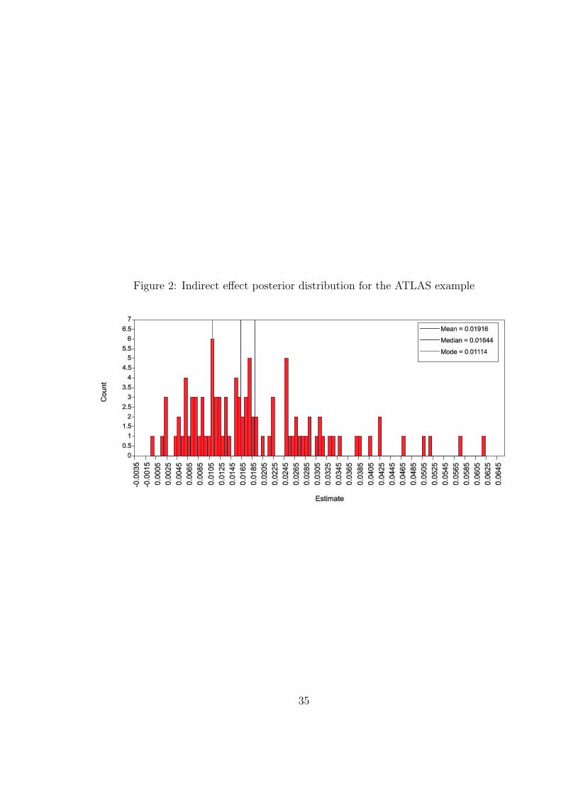
Figure 2: Indirect effect posterior distribution for the ATLAS example

35

Figure 3: Kernel density estimate of indirect effect posterior distribution for the ATLAS example

36

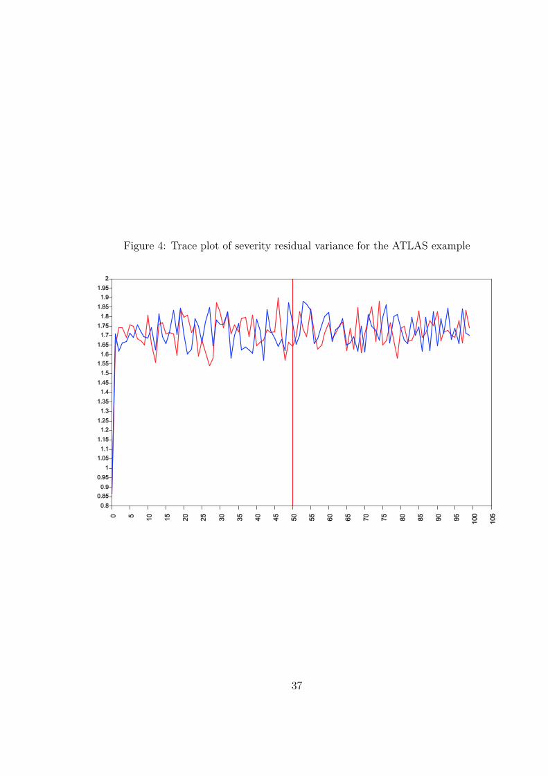
Figure 4: Trace plot of severity residual variance for the ATLAS example

37

Figure 5: Indirect effect posterior distribution from 10,000 iterations for the ATLAS example

38

Figure 6: Autocorrelation plot for indirect effect from 10,000 iterations for the ATLAS example

39

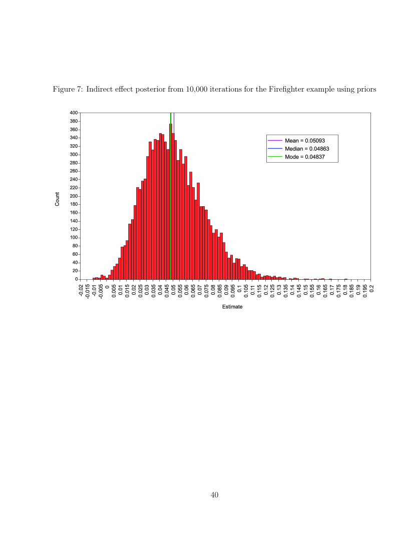
Figure 7: Indirect effect posterior from 10,000 iterations for the Firefighter example using priors

40

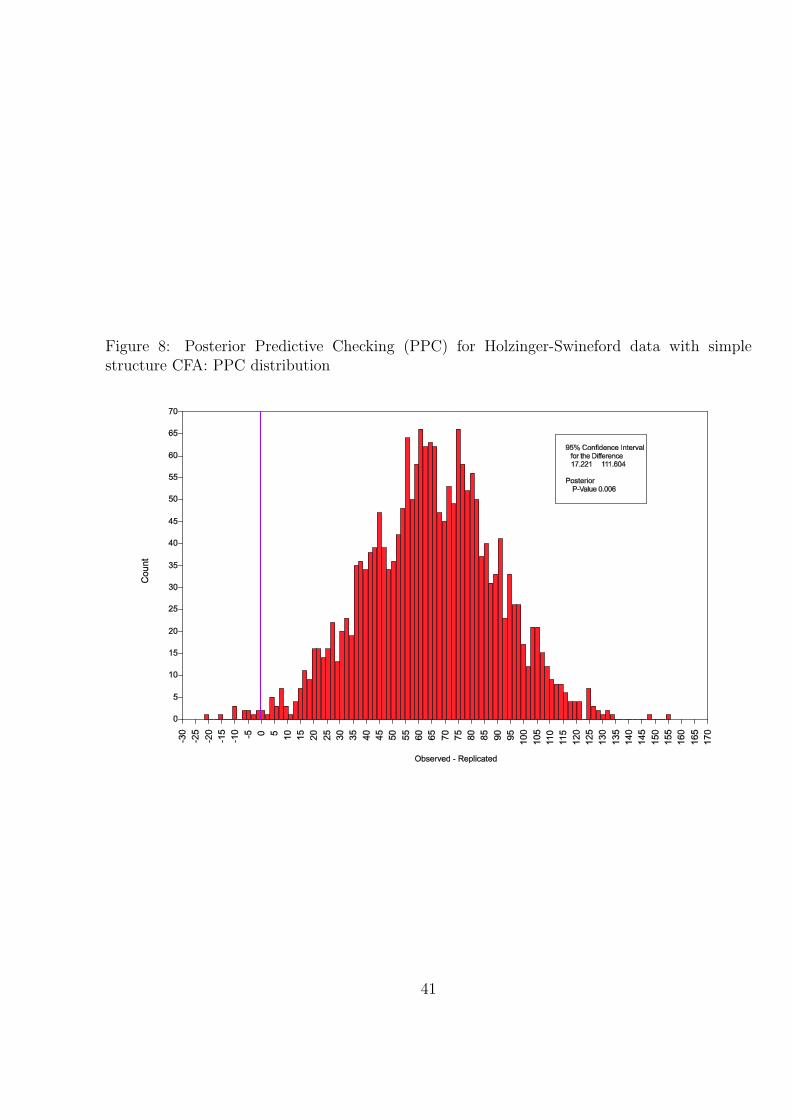
Figure 8: Posterior Predictive Checking (PPC) for Holzinger-Swineford data with simplestructure CFA: PPC distribution

41

Figure 9: Posterior Predictive Checking (PPC) for Holzinger-Swineford data with simplestructure CFA: PPC scatter plot

42

(a) PPC distribution for Bayes CFA

(b) PPC scatterplot for Bayes CFA

Figure 10: Posterior Predictive Checking (PPC) for Holzinger-Swineford data with priors oncross-loadings

43

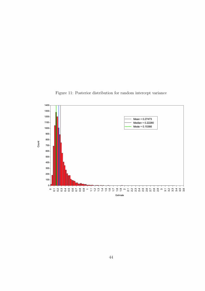
Figure 11: Posterior distribution for random intercept variance

44

Figure 12: Posterior distribution for intraclass correlation

45

Figure 13: Two-part growth modeling of heavy drinking ages 18 - 25

46

Figure 14: Binary multiple-indicator growth modeling of aggressive behavior over eight timepoints

47

Figure 15: Polytomous multiple-indicator, two-level growth modeling of aggressive behavior overeight time points

48

List of Tables

1 Input for Bayes analysis of the Atlas example . . . . . . . . . . . . . 512 Output excerpts for Bayes analysis of the Atlas example . . . . . . . 523 TECH8 iterations with PSR for the first 1000 iterations of the 10,000

iterations analysis of the ATLAS example . . . . . . . . . . . . . . . 534 Output excerpts from Bayesian analysis using 10,000 iterations for the

ATLAS example . . . . . . . . . . . . . . . . . . . . . . . . . . . . . . 545 Input for Bayesian analysis of Firefighter example . . . . . . . . . . . 556 Output excerpts for Bayesian analysis of Firefighter example . . . . . 567 Input for Bayesian analysis with priors for Firefighter example . . . . 578 Output excerpts for Bayesian analysis with priors for Firefighter example 589 Holzinger-Swineford’s hypothesized four domains measured by 19 tests 5910 Input for Bayes CFA . . . . . . . . . . . . . . . . . . . . . . . . . . . 6011 Bayes CFA output excerpts: Model testing . . . . . . . . . . . . . . . 6112 Bayes CFA output excerpts: Model results . . . . . . . . . . . . . . . 6213 Input excerpts for Bayes CFA with informative priors on cross-loadings 6314 Output excerpts for Bayes CFA with informative priors on cross-loadings 6415 Output excerpts for Bayes CFA with informative priors on cross-loadings 6516 Output excerpts for Bayes CFA with informative priors on cross-

loadings (continued) . . . . . . . . . . . . . . . . . . . . . . . . . . . 6617 Input excerpts for Bayes CFA with three free cross-loadings . . . . . 6718 Output excerpts for Bayes CFA with three free cross-loadings . . . . 6819 Output excerpts for Bayes CFA with three free cross-loadings (con-

tinued) . . . . . . . . . . . . . . . . . . . . . . . . . . . . . . . . . . . 6920 Output excerpts for Bayes CFA with three free cross-loadings (con-

tinued) . . . . . . . . . . . . . . . . . . . . . . . . . . . . . . . . . . . 7021 Model testing results for Holzinger-Swineford data (n = 145) . . . . . 7122 Input for Bayes twolevel regression . . . . . . . . . . . . . . . . . . . 7223 Output excerpts for Bayes twolevel regression . . . . . . . . . . . . . 7324 Output excerpts for ML twolevel regression . . . . . . . . . . . . . . . 7425 Output excepts for ML in a Monte Carlo study of a twolevel regression

model . . . . . . . . . . . . . . . . . . . . . . . . . . . . . . . . . . . 7526 Input for for Bayes Monte Carlo twolevel regression using an IG(0.001,

0.001) prior . . . . . . . . . . . . . . . . . . . . . . . . . . . . . . . . 7627 Output excerpts for Bayes Monte Carlo twolevel regression using an

IG(0.001, 0.001) prior . . . . . . . . . . . . . . . . . . . . . . . . . . . 7728 Output excerpts for Bayes Monte Carlo twolevel regression using a

U(0, 1000) prior . . . . . . . . . . . . . . . . . . . . . . . . . . . . . . 7829 Output excerpts for Bayes Monte Carlo twolevel regression using a

IG(-1,0) prior . . . . . . . . . . . . . . . . . . . . . . . . . . . . . . . 79

49

30 Input for Bayesian analysis of a two-part growth model . . . . . . . . 8031 Output excerpts for Bayesian analysis of a two-part growth model:

Model testing . . . . . . . . . . . . . . . . . . . . . . . . . . . . . . . 8132 Output excerpts for Bayesian analysis of a two-part growth model . . 8233 Output excerpts for Bayesian analysis of a two-part growth model,

continued . . . . . . . . . . . . . . . . . . . . . . . . . . . . . . . . . 8334 Output excerpts for ML analysis of a two-part growth model . . . . . 8435 Output excerpts for ML analysis of a two-part growth model, continued 8536 Input for Bayes multiple-indicator growth modeling . . . . . . . . . . 8637 Input for Bayes multiple-indicator growth modeling, continued . . . . 8738 Output excerpts for Bayes multiple-indicator growth modeling . . . . 8839 Output excerpts for Bayes multiple-indicator growth modeling, con-

tinued . . . . . . . . . . . . . . . . . . . . . . . . . . . . . . . . . . . 8940 Output excerpts for Bayes multiple-indicator growth modeling, con-



tinued . . . . . . . . . . . . . . . . . . . . . . . . . . . . . . . . . . . 92

50

Table 1: Input for Bayes analysis of the Atlas example

TITLE: ATLAS, Step 1DATA: FILE = mbr2004atlas.txt;VARIABLE: NAMES = obs group severity nutrit;

USEV = group - nutrit;ANALYSIS: ESTIMATOR = BAYES;

PROCESS = 2;MODEL: severity ON group (a);

nutrit ON severity (b)group;

MODEL CONSTRAINT:NEW (indirect);indirect = a*b;

OUTPUT: TECH1 TECH8 STANDARDIZED;PLOT: TYPE = PLOT2;

51

Table 2: Output excerpts for Bayes analysis of the Atlas example

Posterior One-Tailed 95% C.I.Parameter Estimate S.D. P-Value Lower 2.5% Upper 2.5%

severity ON

group 0.282 0.106 0.010 0.095 0.486

nutrit ON

severity 0.067 0.031 0.000 0.015 0.125group -0.011 0.089 0.440 -0.180 0.155

Intercepts

severity 5.641 0.072 0.000 5.513 5.779nutrit 3.698 0.191 0.000 3.309 4.108

Residual Variances

severity 1.722 0.072 0.000 1.614 1.868nutrit 1.331 0.070 0.000 1.198 1.468

New/Additional Parameters

indirect 0.016 0.013 0.010 0.002 0.052

52

Table 3: TECH8 iterations with PSR for the first 1000 iterations of the 10,000 iterations analysisof the ATLAS example

Potential Parameter WithIteration Scale Reduction Highest PSR

100 1.037 2200 1.014 4300 1.002 2400 1.003 3500 1.002 7600 1.002 6700 1.000 6800 1.003 1900 1.002 11000 1.002 1

53

Table 4: Output excerpts from Bayesian analysis using 10,000 iterations for the ATLAS example


severity ON

group 0.272 0.089 0.001 0.098 0.448

nutrit ON

severity 0.074 0.030 0.008 0.014 0.133group -0.018 0.080 0.408 -0.177 0.140

Intercepts

severity 5.648 0.062 0.000 5.525 5.768nutrit 3.663 0.177 0.000 3.313 4.014

Residual Variances

severity 1.719 0.083 0.000 1.566 1.895nutrit 1.333 0.065 0.000 1.215 1.467


indirect 0.019 0.011 0.009 0.003 0.045

54

Table 5: Input for Bayesian analysis of Firefighter example

TITLE: Yuan and MacKinnon firefighters mediation usingBayesian analysisElliot DL, Goldberg L, Kuehl KS, et al. The PHLAMEStudy: process and outcomes of 2 models of behaviorchange. J Occup Environ Med. 2007; 49(2): 204-213.

DATA: FILE = fire.dat;VARIABLE: NAMES = y m x;MODEL: m ON x (a);

y ON m (b)x;

ANALYSIS: ESTIMATOR = BAYES;PROCESS = 2 ;FBITER = 10000;

MODEL CONSTRAINT:NEW(indirect);indirect = a*b;

OUTPUT: TECH1 TECH8;PLOT: TYPE = PLOT2;

55

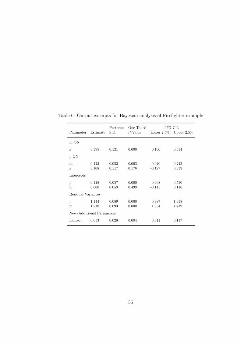
Table 6: Output excerpts for Bayesian analysis of Firefighter example


m ON

x 0.395 0.121 0.000 0.160 0.634

y ON

m 0.142 0.052 0.003 0.040 0.243x 0.108 0.117 0.176 -0.127 0.339

Intercepts

y 0.418 0.057 0.000 0.308 0.530m 0.000 0.059 0.499 -0.115 0.116

Residual Variances

y 1.144 0.089 0.000 0.987 1.338m 1.218 0.093 0.000 1.054 1.419


indirect 0.053 0.028 0.004 0.011 0.117

56

Table 7: Input for Bayesian analysis with priors for Firefighter example

TITLE: Yuan and MacKinnon firefighters mediation usingBayesian analysisElliot DL, Goldberg L, Kuehl KS, et al. The PHLAMEStudy: process and outcomes of 2 models of behaviorchange. J Occup Environ Med. 2007; 49(2): 204-213.

DATA: FILE = fire.dat;VARIABLE: NAMES = y m x;MODEL: m ON x (a);

y ON m (b)x;

ANALYSIS: ESTIMATOR = BAYES;PROCESS = 2;FBITER = 10000;

MODEL PRIORS:a ∼ N (0.35, 0.04);b ∼ N (0.1, 0.01);

MODEL CONSTRAINT:NEW(indirect);indirect = a*b;


57

Table 8: Output excerpts for Bayesian analysis with priors for Firefighter example


m ON

x 0.383 0.104 0.000 0.182 0.588

y ON

m 0.133 0.046 0.003 0.042 0.223x 0.112 0.117 0.169 -0.124 0.341

Intercepts

y 0.418 0.056 0.000 0.308 0.530m 0.000 0.059 0.499 -0.115 0.116

Residual Variances

y 1.143 0.089 0.000 0.986 1.338m 1.218 0.093 0.000 1.053 1.418


indirect 0.049 0.023 0.003 0.012 0.102

58

Table 9: Holzinger-Swineford’s hypothesized four domains measured by 19 tests

Factor loading pattern

Spatial Verbal Speed Memory

visual X 0 0 0cubes X 0 0 0paper X 0 0 0flags X 0 0 0general 0 X 0 0paragrap 0 X 0 0sentence 0 X 0 0wordc 0 X 0 0wordm 0 X 0 0addition 0 0 X 0code 0 0 X 0counting 0 0 X 0straight 0 0 X 0wordr 0 0 0 Xnumberr 0 0 0 Xfigurer 0 0 0 Xobject 0 0 0 Xnumberf 0 0 0 Xfigurew 0 0 0 X

59

Table 10: Input for Bayes CFA

TITLE: Bayes CFA on 19 variables from Holzinger-SwinefordDATA: FILE = holzingr.dat;

FORMAT = f3,2f2,f3,2f2/3x,13(1x,f3)/3x,13(1x,f3);VARIABLE NAMES = id female grade agey agem school visual

cubes paper flags general paragrap sentence wordc wordmaddition code counting straight wordr numberr figurerobject numberf figurew deduct numeric problemr seriesarithmet paperrev flagssub; ! flags = lozengesUSEV = visual cubes paper flags general paragrap sentencewordc wordm addition code counting straight wordrnumberr figurer object numberf figurew;USEOBS = school EQ 0;

DEFINE: visual = visual/sqrt(47.471);cubes = cubes/sqrt (19.622);paper = paper/sqrt(7.908);flags = flags/sqrt(68.695);general = general/sqrt(134.970);paragrap = paragrap/sqrt(11.315);sentence = sentence/sqrt(21.467);wordc = wordc/sqrt(28.505);wordm = wordm/sqrt(62.727);addition = addition/sqrt(561.692);code = code/sqrt(275.759);counting = counting/sqrt(437.752);straight = straight/sqrt(1362.158);wordr = wordr/sqrt(116.448);numberr = numberr/sqrt(56.496);figurer = figurer/sqrt(45.937);object = object/sqrt(20.730);numberf = numberf/sqrt(20.150);figurew = figurew/sqrt(12.845);

ANALYSIS: ESTIMATOR = BAYES;PROCESS = 2;FBITER = 20000;STVAL = ML;

MODEL: spatial BY visual* cubes paper flags;verbal BY general* paragrap sentence wordc wordm;speed BY addition* code counting straight;memory BY wordr* numberr figurer object numberffigurew;spatial-memory@1;

OUTPUT: TECH1 TECH8 STDYX;PLOT: TYPE = PLOT2;

60

Table 11: Bayes CFA output excerpts: Model testing

Tests of model fit

Bayesian Posterior Predictive Checking using Chi-Square95% Confidence Interval for the Difference Between the Observedand the Replicated Chi-Square Values

17.221 111.604Posterior Predictive P-Value 0.006

Information CriterionNumbers of Free Parameters 63Deviance (DIC) 6997.386Estimated Number of Parameters (pD) 63.641

61

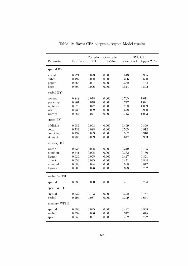
Table 12: Bayes CFA output excerpts: Model results


spatial BY

visual 0.721 0.093 0.000 0.543 0.905cubes 0.497 0.098 0.000 0.306 0.690paper 0.568 0.097 0.000 0.382 0.764flags 0.700 0.096 0.000 0.514 0.892

verbal BY

general 0.848 0.078 0.000 0.705 1.011paragrap 0.861 0.078 0.000 0.717 1.021sentence 0.878 0.077 0.000 0.738 1.039wordc 0.730 0.082 0.000 0.578 0.900wordm 0.884 0.077 0.000 0.743 1.043

speed BY

addition 0.682 0.093 0.000 0.499 0.869code 0.732 0.088 0.000 0.565 0.912counting 0.732 0.089 0.000 0.562 0.910straight 0.785 0.089 0.000 0.617 0.963

memory BY

wordr 0.538 0.098 0.000 0.349 0.735numberr 0.541 0.095 0.000 0.362 0.736figurer 0.629 0.095 0.000 0.447 0.821object 0.653 0.095 0.000 0.471 0.844numberf 0.688 0.094 0.000 0.508 0.877figurew 0.508 0.096 0.000 0.323 0.702

verbal WITH

spatial 0.635 0.080 0.000 0.461 0.764

speed WITH

spatial 0.632 0.103 0.000 0.392 0.787verbal 0.496 0.087 0.000 0.309 0.651

memory WITH

spatial 0.693 0.095 0.000 0.492 0.868verbal 0.532 0.086 0.000 0.342 0.675speed 0.653 0.081 0.000 0.482 0.792

62

Table 13: Input excerpts for Bayes CFA with informative priors on cross-loadings


MODEL: spatial BY visual* cubes paper flags;verbal BY general* paragrap sentence wordc wordm;speed BY addition* code counting straight;memory BY wordr* numberr figurer object numberffigurew;spatial-memory@1;spatial BY general-figurew*0 (a1-a15);verbal BY visual-flags*0 (b1-b4);verbal BY addition-figurew*0 (b5-b14);speed BY visual-wordm*0 (c1-c9);speed BY wordr-figurew*0 (c10-c15);memory BY visual-straight*0 (d1-d13);

MODEL PRIORS:a1-a15 ∼ N(0,.01);b1-b14 ∼ N(0,.01);c1-c15 ∼ N(0,.01);d1-d13 ∼ N(0,.01);


63

Table 14: Output excerpts for Bayes CFA with informative priors on cross-loadings

Tests of model fit


-39.871 61.365Posterior Predictive P-Value 0.353

Information CriterionNumber of Free Parameters 120Deviance (DIC) 6966.543Estimated Number of Parameters (pD) 85.406

64

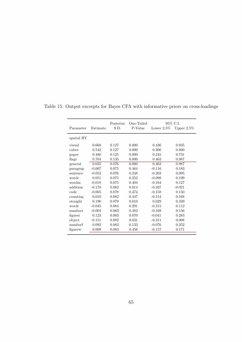
Table 15: Output excerpts for Bayes CFA with informative priors on cross-loadings


spatial BY

visual 0.668 0.127 0.000 0.436 0.935cubes 0.542 0.127 0.000 0.300 0.800paper 0.480 0.125 0.000 0.245 0.731flags 0.704 0.135 0.000 0.463 0.987general 0.035 0.076 0.000 0.463 0.987paragrap -0.007 0.075 0.464 -0.116 0.183sentence -0.052 0.076 0.248 -0.203 0.095wordc 0.051 0.075 0.252 -0.098 0.199wordm -0.018 0.075 0.404 -0.164 0.127addition -0.178 0.082 0.014 -0.337 -0.021code -0.005 0.078 0.474 -0.158 0.150counting 0.010 0.082 0.447 -0.154 0.168straight 0.190 0.079 0.010 0.029 0.339wordr -0.045 0.084 0.291 -0.215 0.112numberr -0.004 0.083 0.482 -0.169 0.156figurer 0.123 0.083 0.070 -0.041 0.283object -0.151 0.082 0.031 -0.311 0.008numberf 0.092 0.083 0.133 -0.076 0.252figurew 0.009 0.083 0.456 -0.157 0.171

65

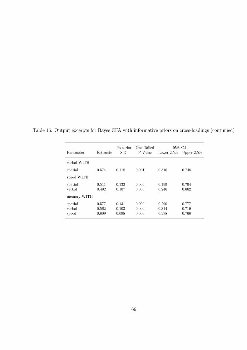
Table 16: Output excerpts for Bayes CFA with informative priors on cross-loadings (continued)


verbal WITH

spatial 0.574 0.118 0.001 0.310 0.748

speed WITH

spatial 0.511 0.132 0.000 0.199 0.704verbal 0.492 0.107 0.000 0.246 0.662

memory WITH


66

Table 17: Input excerpts for Bayes CFA with three free cross-loadings


MODEL: spatial BY visual* cubes paper flags;verbal BY general* paragrap sentence wordc wordm;speed BY addition* code counting straight;memory BY wordr* numberr figurer object numberffigurew;spatial-memory@1;spatial BY addition straight object;


67

Table 18: Output excerpts for Bayes CFA with three free cross-loadings

Tests of model fit



Information CriterionNumber of Free Parameters 66Deviance (DIC) 6957.757Estimated Number of Parameters (pD) 65.223

68

Table 19: Output excerpts for Bayes CFA with three free cross-loadings (continued)


spatial BY

visual 0.768 0.090 0.000 0.598 0.949cubes 0.511 0.097 0.000 0.325 0.709paper 0.583 0.095 0.000 0.398 0.771flags 0.701 0.091 0.000 0.526 0.886addition -0.402 0.171 0.001 -0.834 -0.136straight 0.349 0.104 0.001 0.138 0.550object -0.660 0.272 0.000 -1.317 -0.273

verbal BY

general 0.851 0.078 0.000 0.707 1.013paragrap 0.864 0.077 0.000 0.722 1.022sentence 0.883 0.077 0.000 0.742 1.042wordc 0.734 0.082 0.000 0.580 0.903wordm 0.888 0.077 0.000 0.745 1.047

speed BY

addition 1.024 0.167 0.000 0.757 1.430code 0.705 0.089 0.000 0.537 0.884counting 0.748 0.086 0.000 0.588 0.925straight 0.544 0.102 0.000 0.349 0.750

memory BY

wordr 0.513 0.095 0.000 0.331 0.703numberr 0.514 0.095 0.000 0.332 0.705figurer 0.620 0.093 0.000 0.445 0.807object 1.208 0.268 0.000 0.829 1.849numberf 0.682 0.089 0.000 0.515 0.865figurew 0.499 0.095 0.000 0.316 0.692

69

Table 20: Output excerpts for Bayes CFA with three free cross-loadings (continued)


verbal WITH

spatial 0.575 0.076 0.000 0.407 0.708

speed WITH

spatial 0.598 0.101 0.000 0.379 0.769verbal 0.505 0.087 0.000 0.314 0.657

memory WITH


70

Table 21: Model testing results for Holzinger-Swineford data (n = 145)

Model DIC PPC 95% CI PPC p-value ML p-value

1. CFA 6997 17 - 112 0.006 0.00022. CFA + priors 6967 -40 - 61 0.353 -3. CFA + 3 free 6958 -26 - 70 0.173 0.0494. CFA + 3 free + priors 6955 -49 - 51 0.478 -

71

Table 22: Input for Bayes twolevel regression

TITLE:DATA: FILE = c10n50icc1.dat;VARIABLES: NAMES = y x clus;

WITHIN = x;CLUSTER = clus;

ANALYSIS: TYPE = TWOLEVEL;ESTIMATOR = BAYES;PROCESS = 2;FBITER = 10000;

MODEL: %WITHIN%y ON x;y (w);%BETWEEN%y (b);

MODEL PRIORS:b∼IG(.001,.001);

MODEL CONSTRAINT:NEW(icc);icc = b/(b+w);


72

Table 23: Output excerpts for Bayes twolevel regression

Posterior. One-Tailed 95% C.I.Parameter Estimate S.D. P-Value Lower 2.5% Upper 2.5%

Within Level

y ON

x 0.909 0.069 0.000 0.777 1.042

Residual variances

y 2.105 0.135 0.000 1.866 2.394

Between Level

Means

y 0.145 0.178 0.191 -0.209 0.493

Variances

y 0.223 0.205 0.000 0.073 0.805


ICC 0.096 0.063 0.000 0.033 0.276

73

Table 24: Output excerpts for ML twolevel regression

Two-TailedParameter Estimate S.E. Est./S.E. P-Value

Within Level

y ON

x 0.909 0.069 13.256 0.000

Residual variances

y 2.089 0.133 15.653 0.000

Between Level

Means

y 0.143 0.152 0.942 0.346

Variances

y 0.190 0.104 1.828 0.067


ICC 0.083 0.042 1.975 0.048

74

Table 25: Output excepts for ML in a Monte Carlo study of a twolevel regression model

Estimates S.E. M.S.E. 95% % SigParameter Population Average Std.Dev. Average Cover Coeff

Within Level

y ON

x 1.000 0.9957 0.0630 0.0639 0.0040 0.948 1.000

Residual variances

y 2.000 2.0052 0.1291 0.1281 0.0167 0.946 1.000

Between Level

Means

y 0.000 -0.0035 0.1624 0.1485 0.0263 0.892 0.108

Variances

y 0.222 0.1932 0.1155 0.1045 0.0141 0.808 0.180


ICC 0.100 0.0860 0.0458 0.0422 0.0023 0.812 0.498

75

Table 26: Input for for Bayes Monte Carlo twolevel regression using an IG(0.001, 0.001) prior

TITLE: Bayes IG (eps,eps)MONTECARLO:

NAMES = y x;NOBS = 500;NREP = 500;NCSIZES = 1;CSIZES = 10 (50);WITHIN = x;

MODEL POPULATION:%WITHIN%x*1;y ON x*1;y*2;%BETWEEN%y*.222; !icc = .222/2.222 = 0.1

ANALYSIS: TYPE = TWOLEVEL;ESTIMATOR = BAYES;PROCESS = 2;FBITER = 1000;

MODEL: %WITHIN%y ON x*1;y*2 (w);%BETWEEN%y*.222 (b); !icc = .222/2.222 = 0.1

MODEL PRIORS:b∼IG(.001,.001);

MODEL CONSTRAINT:NEW(icc*.1);icc = b/(w+b);

OUTPUT: TECH9;

76

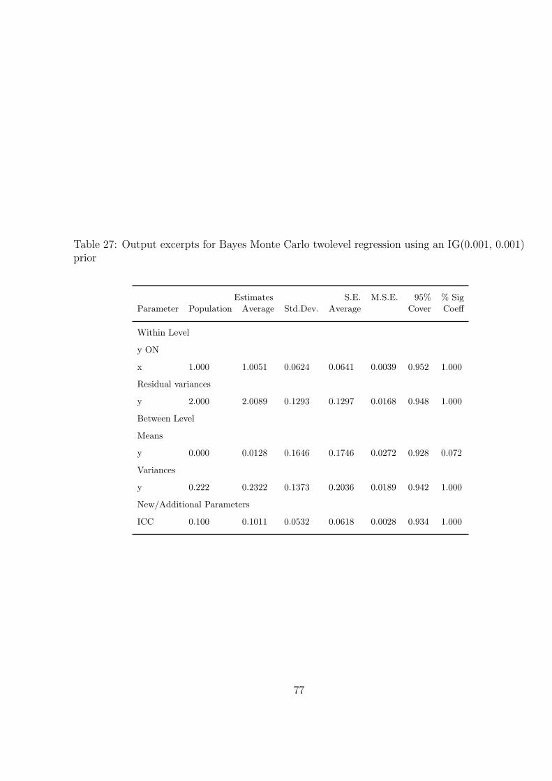
Table 27: Output excerpts for Bayes Monte Carlo twolevel regression using an IG(0.001, 0.001)prior


Within Level

y ON

x 1.000 1.0051 0.0624 0.0641 0.0039 0.952 1.000

Residual variances

y 2.000 2.0089 0.1293 0.1297 0.0168 0.948 1.000

Between Level

Means

y 0.000 0.0128 0.1646 0.1746 0.0272 0.928 0.072

Variances

y 0.222 0.2322 0.1373 0.2036 0.0189 0.942 1.000


ICC 0.100 0.1011 0.0532 0.0618 0.0028 0.934 1.000

77

Table 28: Output excerpts for Bayes Monte Carlo twolevel regression using a U(0, 1000) prior


Within Level

y ON

x 1.000 1.0059 0.0641 0.0640 0.0041 0.954 1.000

Residual variances

y 2.000 1.9992 0.1314 0.1291 0.0172 0.946 1.000

Between Level

Means

y 0.000 0.0190 0.1645 0.2106 0.0277 0.966 0.034

Variances

y 0.222 0.2304 0.1246 0.3255 0.0156 0.930 1.000


ICC 0.100 0.1012 0.0484 0.0841 0.0023 0.928 1.000

78

Table 29: Output excerpts for Bayes Monte Carlo twolevel regression using a IG(-1,0) prior


Within Level

y ON

x 1.000 1.0049 0.0626 0.0640 0.0039 0.946 1.000

Residual variances

y 2.000 2.0061 0.1286 0.1295 0.0165 0.946 1.000

Between Level

Means

y 0.000 0.0123 0.1645 0.2122 0.0272 0.966 0.034

Variances

y 0.222 0.3348 0.1784 0.3767 0.0445 0.928 1.000


ICC 0.100 0.1391 0.0626 0.0876 0.0054 0.928 1.000

79

Table 30: Input for Bayesian analysis of a two-part growth model

TITLE:nlsy36425x25dep.inpcohort 64centering at 25hd82-hd89 (ages 18 - 25)log age scale: x t = a*(ln(t-b) - ln(c-b)), where t is time,a and b are constants to fit the mean curve (chosen as a =2 and b = 16), and c is the centering age, here set at 25.

DATA: FILE = big.dat;FORMAT = 2f5, f2, t14, 5f7, t50, f8, t60, 6f1.0, t67, 2f2.0,t71, 8f1.0, t79, f2.0, t82, 4f2.0;

DATA TWOPART:NAMES = hd82-hd89;BINARY = bin1-bin5;CONTINUOUS = cont1-cont5;

VARIABLE: NAMES = id houseid cohort weight82 weight83 weight84weight88 weight89 weight94 hd82 hd83 hd84 hd88 hd89hd94 dep89 dep94 male black hisp es fh1 fh23 fh123 hsdrpcoll ed89 ed94 cd89 cd94;USEOBSERVATIONS = cohort EQ 64 AND (coll GT 0AND coll LT 20);USEV = male black hisp es fh123hs hsdrp coll bin1-bin5cont1-cont5;CATEGORICAL = bin1-bin5;MISSING = .;AUXILIARY = hd82-hd89;

DEFINE: CUT coll (12.1);ANALYSIS: ESTIMATOR = BAYES;

PROCESS = 2;MODEL: iu su qu | [email protected] [email protected] [email protected] [email protected]

[email protected];iy sy qy | [email protected] [email protected] [email protected] [email protected] [email protected];iu-qy ON male black hisp es fh123 hsdrp coll;

OUTPUT: TECH1 TECH8 STANDARDIZED;PLOT: TYPE = PLOT3;

SERIES = cont1-cont5(sy) | bin1-bin5(su);

80

Table 31: Output excerpts for Bayesian analysis of a two-part growth model: Model testing

Tests of model fit

Number of Free Parameters 74Bayesian Posterior Predictive Checking using Chi-Square

95% Confidence Interval for the Difference Between the Observedand the Replicated Chi-Square Values


81

Table 32: Output excerpts for Bayesian analysis of a two-part growth model

Parameter Estimate Posterior One-Tailed 95% C.I.S.D. P-Value Lower 2.5% Upper 2.5%

iu ON

male 1.649 0.171 0.000 1.324 1.993black -0.742 0.193 0.00 -1.136 -0.381hisp -0.390 0.221 0.036 -0.834 0.038es 0.506 0.204 0.006 0.103 0.903fh123 0.319 0.244 0.095 -0.158 0.796hsdrp -0.196 0.200 0.165 -0.593 0.192coll -0.330 0.186 0.035 -0.701 0.026

iy ON

male 0.357 0.070 0.000 0.222 0.490black -0.143 0.067 0.014 -0.274 -0.016hisp -0.162 0.075 0.015 -0.308 -0.015es 0.106 0.065 0.048 -0.020 0.235fh123 0.217 0.077 0.002 0.068 0.366hsdrp 0.099 0.066 0.070 -0.033 0.224coll -0.038 0.056 0.254 -0.148 0.072

82

Table 33: Output excerpts for Bayesian analysis of a two-part growth model, continued

Parameter Estimate Posterior One-Tailed 95% C.I.S.D. P-Value Lower 2.5% Upper 2.5%

Intercepts

cont1 0.000 0.000 1.000 0.000 0.000cont2 0.000 0.000 1.000 0.000 0.000cont3 0.000 0.000 1.000 0.000 0.000cont4 0.000 0.000 1.000 0.000 0.000cont5 0.000 0.000 1.000 0.000 0.000iu 0.000 0.000 1.000 0.000 0.000su -0.912 0.279 0.000 -1.486 -0.388qu -0.366 0.107 0.000 -0.591 -0.172iy 0.179 0.104 0.033 -0.010 0.381sy -0.268 0.133 0.035 -0.497 0.018qy -0.113 0.046 0.013 -0.198 -0.015

Thresholds

bin1$1 1.395 0.185 0.000 1.028 1.780bin2$1 1.395 0.185 0.000 1.028 1.780bin3$1 1.395 0.185 0.000 1.028 1.780bin4$1 1.395 0.185 0.000 1.028 1.780bin5$1 1.395 0.185 0.000 1.028 1.780

Residual variances

cont1 0.093 0.043 0.000 0.014 0.169cont2 0.199 0.020 0.000 0.164 0.241cont3 0.201 0.021 0.000 0.162 0.244cont4 0.189 0.019 0.000 0.154 0.228cont5 0.176 0.022 0.000 0.134 0.222iu 3.451 0.511 0.000 2.572 4.583su 3.088 0.690 0.000 1.814 4.480qu 0.356 0.104 0.000 0.177 0.568iy 0.215 0.037 0.000 0.147 0.289sy 0.159 0.050 0.000 0.082 0.281qy 0.018 0.006 0.000 0.009 0.033

83

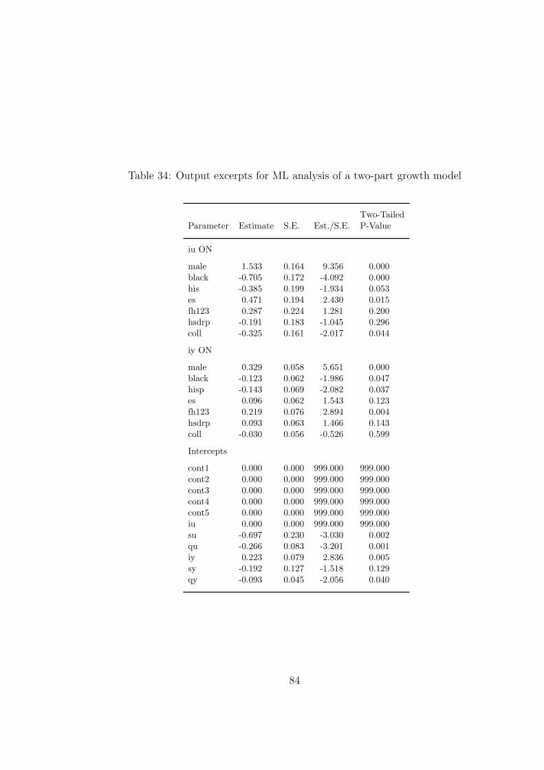
Table 34: Output excerpts for ML analysis of a two-part growth model


iu ON

male 1.533 0.164 9.356 0.000black -0.705 0.172 -4.092 0.000his -0.385 0.199 -1.934 0.053es 0.471 0.194 2.430 0.015fh123 0.287 0.224 1.281 0.200hsdrp -0.191 0.183 -1.045 0.296coll -0.325 0.161 -2.017 0.044

iy ON

male 0.329 0.058 5.651 0.000black -0.123 0.062 -1.986 0.047hisp -0.143 0.069 -2.082 0.037es 0.096 0.062 1.543 0.123fh123 0.219 0.076 2.894 0.004hsdrp 0.093 0.063 1.466 0.143coll -0.030 0.056 -0.526 0.599

Intercepts

cont1 0.000 0.000 999.000 999.000cont2 0.000 0.000 999.000 999.000cont3 0.000 0.000 999.000 999.000cont4 0.000 0.000 999.000 999.000cont5 0.000 0.000 999.000 999.000iu 0.000 0.000 999.000 999.000su -0.697 0.230 -3.030 0.002qu -0.266 0.083 -3.201 0.001iy 0.223 0.079 2.836 0.005sy -0.192 0.127 -1.518 0.129qy -0.093 0.045 -2.056 0.040

84

Table 35: Output excerpts for ML analysis of a two-part growth model, continued


Thresholds

bin1$1 1.273 0.164 7.767 0.000bin2$1 1.273 0.164 7.767 0.000bin3$1 1.273 0.164 7.767 0.000bin4$1 1.273 0.164 7.767 0.000bin5$1 1.273 0.164 7.767 0.000

Residual variances

cont1 0.095 0.052 1.807 0.071cont2 0.199 0.020 10.112 0.000cont3 0.203 0.022 9.276 0.000cont4 0.183 0.018 10.228 0.000cont5 0.169 0.022 7.740 0.000iu 2.863 0.459 6.243 0.000su 1.945 0.489 3.978 0.000qu 0.184 0.061 3.015 0.003iy 0.189 0.032 5.998 0.000sy 0.135 0.058 2.306 0.021qy 0.015 0.008 1.956 0.050

85

Table 36: Input for Bayes multiple-indicator growth modeling

TITLE: Hopkins Cohort 1 All time points with ClassroomInformation

DATA: FILE = Cohort1 classroom ALL.DAT;VARIABLE: NAMES = PRCID stub1F bkRule1F harmO1F bkThin1F

yell1F takeP1F fight1F lies1F tease1F stub1S bkRule1SharmO1S bkThin1S yell1S takeP1S fight1S lies1S tease1Sstub2S bkRule2S harmO2S bkThin2S yell2S takeP2Sfight2S lies2S tease2S stub3S bkRule3S harmO3S bk-Thin3S yell3S takeP3S fight3S lies3S tease3S stub4SbkRule4S harmO4S bkThin4S yell4S takeP4S fight4Slies4S tease4S stub5S bkRule5S harmO5S bkThin5S yell5StakeP5S fight5S lies5S tease5S stub6S bkRule6S harmO6SbkThin6S yell6S takeP6S fight6S lies6S tease6S stub7SbkRule7S harmO7S bkThin7S yell7S takeP7S fight7S lies7Stease7S gender race des011 sch011 sec011 juv99 violchldantisocr conductr athort1F harmP1S athort1S harmP2Sathort2S harmP3S athort3S harmP4S athort4S harmP5Sathort5S harmP6S harmP7S athort7S stub2F bkRule2FharmO2F bkThin2F yell2F takeP2F fight2F harmP2Flies2F athort2F tease2F classrm;USEVAR = stub1f-tease7s male;CATEGORICAL = categorical = stub1f-tease7s;MISSING = ALL (999);

DEFINE: cut stub1f-tease7s(1.5);MALE = 2 - gender;

ANALYSIS: PROCESS = 2 ;ESTIMATOR = BAYES;FBITER = 20000;

86

Table 37: Input for Bayes multiple-indicator growth modeling, continued

MODEL: f1 BY stub1fbkrule1f-tease1f (1-8);f2 BY stub1sbkrule1s-tease1s (1-8);f3 BY stub2sbkrule2s-tease2s (1-8);f4 BY stub3sbkrule3s-tease3s (1-8);f5 BY stub4sbkrule4s-tease4s (1-8);f6 BY stub5sbkrule5s-tease5s (1-8);f7 BY stub6sbkrule6s-tease6s (1-8);f8 BY stub7sbkrule7s-tease7s (1-8);[stub1f$1 stub1s$1 stub2s$1 stub3s$1 stub4s$1] (11);[stub5s$1 stub6s$1 stub7s$1] (11);[bkrule1f$1 bkrule1s$1 bkrule2s$1 bkrule3s$1] (12);[bkrule4s$1 bkrule5s$1 bkrule6s$1 bkrule7s$1] (12);[harmo1f$1 harmo1s$1 harmo2s$1 harmo3s$1] (13);[harmo4s$1 harmo5s$1 harmo6s$1 harmo7s$1] (13);[bkthin1f$1 bkthin1s$1 bkthin2s$1 bkthin3s$1] (14);[bkthin4s$1 bkthin5s$1 bkthin6s$1 bkthin7s$1] (14);[yell1f$1 yell1s$1 yell2s$1 yell3s$1 yell4s$1 yell5s$1] (15);[yell6s$1 yell7s$1] (15);[takeP1f$1 takeP1s$1 takeP2s$1 takeP3s$1] (16);[takeP4s$1 takeP5s$1 takeP6s$1 takeP7s$1] (16);[fight1f$1 fight1s$1 fight2s$1 fight3s$1 fight4s$11] (17);[fight5s$1 fight6s$1 fight7s$1] (17);[lies1f$1 lies1s$1 lies2s$1 lies3s$1 lies4s$1 lies5s$1] (18);[lies6s$1 lies7s$1] (18);[tease1f$1 tease1s$1 tease2s$1 tease3s$1 tease4s$1] (19);[tease5s$1 tease6s$1 tease7s$1] (19);[f1-f8@0];i s q | f1@0 [email protected] [email protected] [email protected] [email protected] [email protected] [email protected]@6.5;i-q ON male;

OUTPUT: TECH1 TECH4 TECH8 TECH10 STANDARDIZEDSVALUES;

PLOT: TYPE = PLOT2;

87

Table 38: Output excerpts for Bayes multiple-indicator growth modeling

Tests of model fit

Number of Free Parameters 36Bayesian Posterior Predictive Checking using Chi-Square

95% Confidence Interval for the Difference Between the Observedand the Replicated Chi-Square Values

129.488 547.650Posterior Predictive P-Value 0.002

88

Table 39: Output excerpts for Bayes multiple-indicator growth modeling, continued


i |

f1 1.000 0.000 0.000 1.000 1.000f2 1.000 0.000 0.000 1.000 1.000f3 1.000 0.000 0.000 1.000 1.000f4 1.000 0.000 0.000 1.000 1.000f5 1.000 0.000 0.000 1.000 1.000f6 1.000 0.000 0.000 1.000 1.000f7 1.000 0.000 0.000 1.000 1.000f8 1.000 0.000 0.000 1.000 1.000

s |

f1 0.000 0.000 1.000 0.000 0.000f2 0.500 0.000 0.000 0.500 0.500f3 1.500 0.000 0.000 1.500 1.500f4 2.500 0.000 0.000 2.500 2.500f5 3.500 0.000 0.000 3.500 3.500f6 4.500 0.000 0.000 4.500 4.500f7 5.500 0.000 0.000 5.500 5.500f8 6.500 0.000 0.000 6.500 6.500

q |

f1 0.000 0.000 1.000 0.000 0.000f2 0.250 0.000 0.000 0.250 0.250f3 2.250 0.000 0.000 2.250 2.250f4 6.250 0.000 0.000 6.250 6.250f5 12.250 0.000 0.000 12.250 12.250f6 20.250 0.000 0.000 20.250 20.250f7 30.250 0.000 0.000 30.250 30.250f8 42.250 0.000 0.000 42.250 42.250

89



f1 BY

stub1f 1.000 0.000 0.000 1.000 1.000bkrule1f 1.395 0.060 0.000 1.288 1.522harmo1f 1.858 0.096 0.000 1.695 2.076bkthin1f 1.335 0.065 0.000 1.221 1.470yell1f 1.182 0.047 0.000 1.097 1.279takep1f 1.416 0.063 0.000 1.311 1.553fight1f 1.416 0.059 0.000 1.308 1.537lies1f 1.323 0.054 0.000 1.227 1.438tease1f 1.294 0.052 0.000 1.196 1.402

f8 BY

stub7s 1.000 0.000 0.000 1.000 1.000bkrule7s 1.395 0.060 0.000 1.288 1.522harmo7s 1.858 0.096 0.000 1.695 2.076bkthin7s 1.335 0.065 0.000 1.221 1.470yell7s 1.182 0.047 0.000 1.097 1.279takep7s 1.416 0.063 0.000 1.311 1.553flight7s 1.416 0.059 0.000 1.308 1.537lies7s 1.323 0.054 0.000 1.227 1.438tease7s 1.294 0.052 0.000 1.196 1.402

i ON

male 0.623 0.092 0.000 0.447 0.803

s ON

male 0.108 0.049 0.012 0.013 0.205

q ON

male -0.015 0.007 0.015 -0.030 -0.001

s WITH

i -0.412 0.057 0.000 -0.530 -0.308

q WITH

i 0.034 0.007 0.000 0.021 0.048s -0.028 0.005 0.000 -0.038 -0.019

90



Intercepts

f1 0.000 0.000 1.000 0.000 0.000f2 0.000 0.000 1.000 0.000 0.000f3 0.000 0.000 1.000 0.000 0.000f4 0.000 0.000 1.000 0.000 0.000f5 0.000 0.000 1.000 0.000 0.000f6 0.000 0.000 1.000 0.000 0.000f7 0.000 0.000 1.000 0.000 0.000f8 0.000 0.000 1.000 0.000 0.000i 0.000 0.000 1.000 0.000 0.000s 0.002 0.034 0.479 -0.067 0.068q 0.002 0.005 0.365 -0.008 0.012

Thresholds

stub1f$1 -0.386 0.067 0.000 -0.523 -0.263bkrule1f$1 -0.215 0.090 0.007 -0.396 -0.038harmo1f$1 1.657 0.142 0.000 1.390 1.951bkthin1f$1 1.813 0.098 0.000 1.645 2.035yell1f$1 0.389 0.078 0.000 0.236 0.546takep1f$1 1.346 0.101 0.000 1.151 1.556fight1f$1 0.834 0.096 0.000 0.638 1.016lies1f$1 0.667 0.088 0.000 0.487 0.837tease1f$1 0.050 0.084 0.273 -0.120 0.209stub7s$1 -0.386 0.067 0.000 -0.523 -0.263bkrule7s$1 -0.215 0.090 0.007 -0.396 -0.038harmo7s$1 1.657 0.142 0.000 1.390 1.951bkthin7s$1 1.813 0.098 0.000 1.645 2.035yell7s$1 0.389 0.078 0.000 0.236 0.546takep7s$1 1.346 0.101 0.000 1.151 1.556fight7s$1 0.834 0.096 0.000 0.638 1.016lies7s$1 0.667 0.088 0.000 0.487 0.837tease7s$1 0.050 0.084 0.273 -0.120 0.209

91



Residual variances

f1 0.147 0.060 0.000 0.032 0.271f2 0.489 0.061 0.000 0.371 0.608f3 1.724 0.170 0.000 1.435 2.099f4 0.866 0.102 0.000 0.680 1.081f5 0.686 0.080 0.000 0.543 0.859f6 0.747 0.087 0.000 0.591 0.933f7 0.961 0.108 0.000 0.771 1.193f8 0.527 0.109 0.000 0.321 0.752i 1.771 0.151 0.000 1.494 2.090s 0.254 0.034 0.000 0.192 0.327q 0.004 0.001 0.000 0.002 0.005

92

bayesian analysis in mplus: a brief introduction 3.pdf · bayesian analysis in mplus: a brief...

Documents